Maximum Selection and Ranking under Noisy Comparisons

Abstract

We consider $(\epsilon,\delta)$-PAC maximum-selection and ranking for general probabilistic models whose comparisons probabilities satisfy strong stochastic transitivity and stochastic triangle inequality. Modifying the popular knockout tournament, we propose a maximum-selection algorithm that uses ${\cal O}{\left({\frac{n}{\epsilon^{2}}\log\frac{1}{\delta}}\right)}$ comparisons, a number tight up to a constant factor. We then derive a general framework that improves the performance of many ranking algorithms, and combine it with merge sort and binary search to obtain a ranking algorithm that uses ${\cal O}{\left({\frac{n\log n(\log\log n)^{3}}{\epsilon^{2}}}\right)}$ comparisons for any $\delta\geq\frac{1}{n}$, a number optimal up to a $(\log\log n)^{3}$ factor.

1 Introduction

1.1 Background

Maximum selection and sorting using pairwise comparisons are computer-science staples taught in most introductory classes and used in many applications. In fact, sorting, also known as ranking, has been claimed to utilize 25% of computer cycles worldwide Mukherjee (2011).

In many applications, the pairwise comparisons produce only random outcomes. For example, sports tournaments rank teams based on pairwise matches, but match outcomes are probabilistic in nature. Patented by Microsoft, TrueSkill Herbrich et al. (2006) is such a ranking system for Xbox gamers. Another important application is online advertising. Prominent web pages devote precious little space to advertisements, limiting companies like Google, Microsoft, or Yahoo! to present a typical user with just a couple of ads, of which the user selects at most one. Based on these small random comparisons, the company would like to rank the ads according to their appeal Radlinski & Joachims (2007); Radlinski et al. (2008).

This and related applications have brought about a resurgence of interest in maximum selection and ranking using noisy comparisons. Several noise models were considered, including the popular Plackett-Luce model Plackett (1975); Luce (2005). Yet even for such specific models, the complexity of maximum selection was known only up to a $\log n$ factor and the complexity of ranking was known only up to a $\log n$ factor. We consider a broader class of models and propose algorithms that are optimal up to a constant factor for maximum selection and up to $(\log\log n)^{3}$ for ranking.

1.2 Notation

Noiseless comparison assumes an unknown underlying ranking $r(1){,}\ldots{,}r(n)$ of the elements such that if two elements are compared, the higher-ranked one is selected. Similarly for noisy comparisons, we assume an unknown ranking of the $n$ elements, but now if two elements $i$ and $j$ are compared, $i$ is chosen with some unknown probability $p(i,j)$ and $j$ is chosen with probability $p(j,i)=1-p(i,j)$, where the higher-ranked element has probability $\geq{\frac{1}{2}}$. Repeated comparisons are independent of each other.

Let $\tilde{p}(i,j)=p(i,j)-\frac{1}{2}$ reflect the additional probability by which $i$ is preferable to $j$. Note that $\tilde{p}(j,i)=-\tilde{p}(i,j)$ and $\tilde{p}(i,j)\geq 0$ if $r(i)>r(j)$. $|\tilde{p}(i,j)|$ can also be seen as a measure of dissimilarity between $i$ and $j$. In our model we assume that two very natural properties hold whenever $r(i)>r(j)>r(k)$.

(1)Strong stochastic transitivity:

$$\tilde{p}(i,k)\geq\max(\tilde{p}(i,j),\tilde{p}(j,k));$$

(2) Stochastic triangle inequality:

$$\tilde{p}(i,k)\leq\tilde{p}(i,j)+\tilde{p}(j,k).$$

These properties are satisfied by several popular preference models e.g., Plackett-Luce(PL) model.

Two types of algorithms have been proposed for finding the maximum and ranking under noisy comparisons: non-adaptive or offline Rajkumar & Agarwal (2014); Negahban et al. (2012, 2016); Jang et al. (2016) where we cannot choose the comparison pairs, and adaptive or online where the comparison pairs are selected sequentially based on previous results. In this paper we focus on the latter.

We specify the desired output via the $(\epsilon,\delta)$-PAC paradigm Yue & Joachims (2011); Busa-Fekete et al. (2014b) that requires the output to likely closely approximate the intended value. Specifically, given $\epsilon,\delta>0$, with probability $\geq 1-\delta$, maximum selection must output an element $i$ such that for $j$ with $r(j)=n$,

$$p(i,j)\geq\frac{1}{2}-\epsilon.$$

We call such an output $\epsilon$-maximum. Similarly, with probability $\geq 1-\delta$, the ranking algorithm must output a ranking $r^{\prime}(1){,}\ldots{,}r^{\prime}(n)$ such that whenever $r^{\prime}(i)>r^{\prime}(j)$,

$$p(i,j)\geq\frac{1}{2}-\epsilon.$$

We call such a ranking $\epsilon$-ranking.

1.3 Paper outline

In Section 2 we mention somerelated works. In Section 3 we highlight our main contributions. In Section 4 we propose the maximum selection algorithm. In Section 5 we propose the ranking algorithm. In Section 6 we provide experiments. In Section  7 we discuss the results and mention some future directions.

2 Related work

Heckel et al. (2016); Urvoy et al. (2013); Busa-Fekete et al. (2014b, b) assume no underlying ranking or constraints on probabilities and find ranking based on Copeland, Borda count and Random Walk procedures.  Urvoy et al. (2013); Busa-Fekete et al. (2014b) showed that if the probabilities $p(i,j)$ are not constrained, both maximum selection and ranking problems require $\Theta(n^{2})$ comparisons. Several models have therefore been considered to further constrain the probabilities.

Under the assumptions of strong stochastic transitivity and triangle inequality , Yue & Joachims (2011) derived a PAC maximum selection algorithm that uses $O{\left({\frac{n}{\epsilon^{2}}\log\frac{n}{\epsilon\delta}}\right)}$ comparisons.  Szörényi et al. (2015) derived a PAC ranking algorithm for PL-model distributions that requires $O(\frac{n}{\epsilon^{2}}\log n\log\frac{n}{\delta\epsilon})$ comparisons.

In addition to PAC paradigm, Yue & Joachims (2011) also considered this problem under the bandit setting and bounded the regret of the resulting dueling bandits problem. Following this work, several other works e.g.  Syrgkanis et al. (2016) looked at similar formulation.

Another non-PAC approach by  Busa-Fekete et al. (2014a); Feige et al. (1994) solves the maximum selection and ranking problems. They assume a lower bound on $|\tilde{p}(i,j)|$ and the number of comparisons depends on this lower bound. If $|\tilde{p}(i,j)|$ is $0$ for any pair, then these algorithms will never terminate.

Several other noise models have also been considered in practice that have either adverserial noise or the stochastic noise that does not obey triangle inequality. For example,  Acharya et al. (2014a, 2016, b) considered adversarial sorting with applications to density estimation and Ajtai et al. (2015) considered the same with deterministic algorithms. Mallows stochastic model Busa-Fekete et al. (2014a) does not satisfy the stochastic triangle inequality and hence our theoretical guarantees do not hold under this model. However our simulations suggest that our algorithm can have a reasonable performance over Mallows model.

3 New results

Recall that we study $(\epsilon,\delta)$-PAC model for the problems of online maximum selection and ranking using pairwise comparisons under strong stochastic transitivity and stochastic triangle inequality assumptions. The goal is to find algorithms that use small number of comparisons. Our main contributions are:

• A maximum selection algorithm that uses $O{\left({\frac{n}{\epsilon^{2}}\log\frac{1}{\delta}}\right)}$ comparisons and therefore our algorithm is optimal up to constants.

• A ranking algorithm that uses at most $O{\left({\frac{n(\log n)^{3}}{\epsilon^{2}}\log\frac{n}{\delta}}\right)}$ comparisons and outputs $\epsilon$-ranking for any $\delta$.

• A framework that given any ranking algorithm with ${\cal O}{\left({\frac{n(\log n)^{x}}{\epsilon^{2}}\log\frac{n}{\delta}}\right)}$ sample complexity, provides a ranking algorithm with ${\cal O}{\left({\frac{n\log n(\log\log n)^{x}}{\epsilon^{2}}}\right)}$ sample complexity for $\delta\geq\frac{1}{n}$.

• Using the framework above, we present an algorithm that uses at most $O{\left({\frac{n\log n(\log\log n)^{3}}{\epsilon^{2}}}\right)}$ comparisons and outputs $\epsilon$-ranking for $\delta=\frac{1}{n}$. We also show a lower bound of $\Omega{\left({\frac{n\log n}{\epsilon^{2}}}\right)}$ on the number of comparisons used by any PAC ranking algorithm, therefore proving our algorithm is optimal up to $\log\log n$ factors.

4 Maximum selection

4.1 Algorithm outline

We propose a simple maximum-selection algorithm based on Knockout tournaments. Knockout tournaments are often used to find a maximum element under non-noisy comparisons. Knockout tournament of $n$ elements runs in ${\lceil{\log n}\rceil}$ rounds where in each round it randomly pairs the remaining elements and proceeds the winners to next round.

Our algorithm, given in Knockout uses ${\cal O}{\left({\frac{n}{\epsilon^{2}}\log\frac{1}{\delta}}\right)}$ comparisons and ${\cal O}(n)$ memory to find an $\epsilon$-maximum. Yue & Joachims (2011) uses ${\cal O}{\left({\frac{n}{\epsilon^{2}}\log\frac{n}{\epsilon\delta}}\right)}$ comparisons and ${\cal O}(n^{2})$ memory to find an $\epsilon$-maximum. Hence we get $\log n$-factor improvement in the number of comparisons and also we use linear memory compared to quadratic memory. Using the lower bound in  Feige et al. (1994), it can be inferred that the best PAC maximum selection algorithm requires $\Omega{\left({\frac{n}{\epsilon^{2}}\log\frac{1}{\delta}}\right)}$ comparisons, hence up to constant factor, Knockout is optimal. Also our algorithm can be parallelized to run in ${\cal O}{\left({\frac{\log n}{\epsilon^{2}}\log\frac{1}{\delta}}\right)}$ time.

Due to the noisy nature of the comparisons, we repeat each comparison several times to gain confidence about the winner. Note that in knockout tournaments, the number of pairs in a round decreases exponentially with each round. Therefore we afford to repeat the comparisons more times in the latter rounds and get higher confidence. Let $b_{i}$ be the highest-ranked element (according to unobserved underlying ranking) at the beginning of round $i$. We repeat the comparisons in round $i$ enough times to ensure that $\tilde{p}(b_{i},b_{i+1})\leq\frac{c\epsilon}{2^{i/3}}$ with probability $\geq 1-\frac{\delta}{2^{i}}$ where $c=2^{1/3}-1$. By the stochastic triangle inequality, $\tilde{p}(b_{1},b_{{\lceil{\log n}\rceil}+1})\leq\sum_{i=1}^{{\lceil{\log n}\rceil}+1}\frac{c\epsilon}{2^{i/3}}\leq\epsilon$ with probability $\geq 1-\delta$.

There is a relaxed notion of strong stochastic transitivity. For $\gamma\geq 1$, $\gamma$-stochastic transitivity Yue & Joachims (2011): if $r(i)>r(j)>r(k)$, then $\max(\tilde{p}(i,j),\tilde{p}(j,k))\leq\gamma\cdot\tilde{p}(i,k)$.

Our results apply to this general notion of $\gamma$-stochastic transitivity and the analysis of Knockout is presented under this model. Yue & Joachims (2011) uses ${\cal O}(\frac{n\gamma^{6}}{\epsilon^{2}}\log\frac{n}{\delta})$ comparisons to find an $\epsilon$-maximum whereas Knockout uses only ${\cal O}(\frac{n\gamma^{2}}{\epsilon^{2}}\log\frac{1}{\delta})$ comparisons. Hence we get a huge improvement in the exponent of $\gamma$ as well as removing the extra $\log n$ factor.

To simplify the analysis, we assume that $n$ is a power of 2, otherwise we can add $2^{{\lceil{\log n}\rceil}}-n$ dummy elements that lose to every original element with probability 1. Note that all $\epsilon$-maximums will still be from the original set.

4.2 Algorithm

We start with a subroutine Compare that compares two elements. It compares two elements $i$, $j$ and maintains empirical probability $\hat{p}_{i}$, a proxy for $p(i,j)$. It also maintains a confidence value $\hat{c}$ s.t., w.h.p., $\hat{p}_{i}\in(p(i,j)-\hat{c},p(i,j)+\hat{c})$. Compare stops if it is confident about the winner or if it reaches its comparison budget $m$. If it reaches $m$ comparisons, it outputs the element with more wins breaking ties randomly.

Algorithm 1 Comprare

Input: element $i$, element $j$, bias $\epsilon$, confidence $\delta$.
Initialize: $\hat{p_{i}}=\frac{1}{2}$, $\hat{c}=\frac{1}{2}$, $m=\frac{1}{2\epsilon^{2}}\log\frac{2}{\delta}$, $r=0$, $w_{i}=0$.

1. while ($|\hat{p_{i}}-\frac{1}{2}|\leq\hat{c}-\epsilon$ and $r\leq m$)

   1. Compare $i$ and $j$. if $i$ wins $w_{i}$ = $w_{i}+1$.

   2. $r=r+1$, $\hat{p_{i}}=\frac{w_{i}}{r}$, $\hat{c}=\sqrt{\frac{1}{2r}\log\frac{4r^{2}}{\delta}}$.

if $\hat{p_{i}}\leq\frac{1}{2}$ Output: j. else Output: i.

We show that the subroutine Compare always outputs the correct winner if the elements are well seperated.

Lemma 1.

If $\tilde{p}(i,j)\geq\epsilon$, then

$$Pr(\textsc{Compare}(i,j,\epsilon,\delta)\neq i)\leq\delta.$$

Note that instead of using fixed number of comparisons, Compare stops the comparisons adaptively if it is confident about the winner. If $|\tilde{p}(i,j)|\gg\epsilon$, Compare stops much before comparison budget $\frac{1}{2\epsilon^{2}}\log\frac{2}{\delta}$ and hence works better in practice.

Now we present the subroutine Knockout-Round that we use in main algorithm Knockout.

4.2.1 Knockout-Round

Knockout-Round takes a set $S$ and outputs a set of size $|S|/2$. It randomly pairs elements, compares each pair using Compare, and returns the set of winners. We will later show that maximum element in the output set will be comparable to maximum element in the input set.

Algorithm 2 Knockout-Round

Input: Set $S$, bias $\epsilon$, confidence $\delta$.
Initialize: Set $O=\emptyset$.

1. Pair elements in $S$ randomly.

2. for every pair $(a,b)$:

   1. Add Compare$(a,b,\epsilon,\delta)$ to $O$.

Output: $O$

Note that comparisons between each pair can be handled by a different processor and hence this algorithm can be easily parallelized.

Note that a set $S$ can have several maximum elements. Comparison probabilities corresponding to all maximum elements will be essentially same because of triangle inequality. We define $\text{max}(S)$ to be the maximum element with the least index, namely,

$$\text{max}(S)\stackrel{{\scriptstyle\mathrm{def}}}{{=}}S\Big{(}{\min\{i:\tilde{p}(S(i),S(j))\geq 0\quad\forall j\}}\Big{)}.$$

Lemma 2.

$\textsc{Knockout-Round}(S,\epsilon,\delta)$ uses $\frac{|S|}{4\epsilon^{2}}\log\frac{2}{\delta}$ comparisons and with probability $\geq 1-\delta$,

$$\tilde{p}\Bigg{(}\text{max}(S),\text{max}\Big{(}\textsc{Knockout-Round}(S,\epsilon,\delta)\Big{)}\Bigg{)}\leq\gamma\epsilon$$

4.2.2 Knockout

Now we present the main algorithm Knockout. Knockout takes an input set $S$ and runs $\log n$ rounds of Knockout-Round halving the size of $S$ at the end of each round. Recall that Knockout-Round makes sure that maximum element in the output set is comparable to maximum element in the input set. Using this, Knockout makes sure that the output element is comparable to maximum element in the input set.

Since the size of $S$ gets halved after each round, Knockout compares each pair more times in the latter rounds. Hence the bias between maximum element in input set and maximum element in output set is small in latter rounds.

Algorithm 3 Knockout

Input: Set $S$, bias $\epsilon$, confidence $\delta$, stochasticity $\gamma$.
Initialize: $i=1$, $S=$ set of all elements, $c=2^{1/3}-1$.
while $|S|>1$

1. $S$ = Knockout-Round${\left({S,\frac{c\epsilon}{\gamma 2^{i/3}},\frac{\delta}{2^{i}}}\right)}$.

2. $i=i+1.$

Output: the unique element in $S$.

Note that Knockout uses only memory of set $S$ and hence ${\cal O}(n)$ memory suffices. Now we bound the number of comparisons used by Knockout and prove the correctness.

Theorem 3.

Knockout$(S,\epsilon,\delta)$ uses ${\cal O}{\left({\frac{\gamma^{2}|S|}{\epsilon^{2}}\log\frac{1}{\delta}}\right)}$ comparisons and with probability at least $1-\delta$, outputs an $\epsilon$-maximum.

5 Ranking

We propose a ranking algorithm that with probability at least $1-\frac{1}{n}$ uses ${\cal O}{\left({\frac{n\log n(\log\log n)^{3}}{\epsilon^{2}}}\right)}$ comparisons and outputs an $\epsilon$-ranking.

Notice that we use only $\tilde{{\cal O}}{\left({\frac{n\log n}{\epsilon^{2}}}\right)}$ comparisons for $\delta=\frac{1}{n}$ where as  Szörényi et al. (2015) uses ${\cal O}{\left({n(\log n)^{2}/\epsilon^{2}}\right)}$ comparisons even for constant error probability $\delta$. Furthermore  Szörényi et al. (2015) provided these guarantees only under Plackett-Luce model which is more restrictive compared to ours. Also, their algorithm uses ${\cal O}(n^{2})$ memory compared to ${\cal O}(n)$ memory requirement of ours.

Our main algorithm Binary-Search-Ranking assumes the existence of a ranking algorithm Rank-$x$ that with probability at least $1-\delta$ uses ${\cal O}{\left({\frac{n}{\epsilon^{2}}(\log n)^{x}\log\frac{n}{\delta}}\right)}$ comparisons and outputs an $\epsilon$-ranking for any $\delta>0$, $\epsilon>0$ and some $x>1$. We also present a Rank-$x$ algorithm with $x=3$.

Observe that we need Rank-$x$ algorithm to work for any model that satisfies strong stochastic transitivity and stochastic triangle inequality. Szörényi et al. (2015) showed that their algorithm works for Plackett-Luce model but not for more general model. So we present a Rank-$x$ algorithm that works for general model.

The main algorithm Binary-Search-Ranking randomly selects $\frac{n}{(\log n)^{x}}$ elements (anchors) and rank them using Rank-$x$ . The algorithm has then effectively created $\frac{n}{(\log n)^{x}}$ bins, each between two successively ranked anchors. Then for each element, the algorithm identifies the bin it belongs to using a noisy binary search algorithm. The algorithm then ranks the elements within each bin using Rank-$x$ .

We first present Merge-Rank, a Rank-3 algorithm.

5.1 Merge Ranking

We present a simple ranking algorithm Merge-Rank that uses ${\cal O}{\left({\frac{n(\log n)^{3}}{\epsilon^{2}}\log\frac{n}{\delta}}\right)}$ comparisons, $O(n)$ memory and with probability $\geq 1-\delta$ outputs an $\epsilon$-ranking. Thus Merge-Rank is a Rank-$x$ algorithm for $x=3$.

Similar to Merge Sort, Merge-Rank divides the elements into two sets of equal size, ranks them separately and combines the sorted arrays. Due to the noisy nature of comparisons, Merge-Rank compares two elements $i,j$ sufficient times, so that the comparison output is correct with high probability when $|\tilde{p}(i,j)|\geq\frac{\epsilon}{\log n}$. Put differently, Merge-Rank is same as the typical Merge Sort, except it uses Compare as the comparison function.

Let’s define the error of an ordered set $S$ as the maximum distance between two wrongly ordered items in $S$, namely,

$$err(S)\stackrel{{\scriptstyle\mathrm{def}}}{{=}}\max_{1\leq i\leq j\leq|S|}\Big{(}{\tilde{p}(S(j),S(i))}\Big{)}.$$

We show that when we merge two ordered sets, the error of the resulting ordered set will be at most $\frac{\epsilon}{\log n}$ more than the maximum of errors of individual ordered sets.

Observe that Merge-Rank is a recursive algorithm and the error of a singleton set is $0$. Two singleton sets each containing a unique element from the input set merge to form a set with two elements with an error at most $\frac{2\epsilon}{\log n}$, then two sets with two elements merge to form a set with four elements with an error of at most $\frac{3\epsilon}{\log n}$ and henceforth. Therefore the error of the output ordered set is bounded by $\epsilon$.

Lemma 4 shows that Merge-Rank can output an $\epsilon$-ranking of $S$ with probability $\geq 1-\delta$. It also bounds the number of comparisons used by the algorithm.

Lemma 4.

$\textsc{Merge-Rank}{\left({S,\frac{\epsilon}{\log|S|},\frac{\delta}{|S|^{2}}}\right)}$ takes ${\cal O}{\left({\frac{|S|(\log|S|)^{3}}{\epsilon^{2}}\log\frac{|S|}{\delta}}\right)}$ comparisons and with probability $\geq 1-\delta$, outputs an $\epsilon$-ranking. Hence, Merge-Rank is a Rank-3 algorithm.

Now we present our main ranking algorithm.

5.2 Binary-Search-Ranking

We first sketch the algorithm outline below. We then provide a proof outline.

5.2.1 Algorithm outline

Our algorithm is stated in Binary-Search-Ranking. It can be summarized in three major parts.

Creating anchors: (Steps $1$ to $3$) Binary-Search-Ranking first selects a set $S^{\prime}$ of $\frac{n}{(\log n)^{x}}$ random elements (anchors) and ranks them using Rank-$x$ . At the end of this part, there are $\frac{n}{(\log n)^{x}}$ ranked anchors. Equivalently, the algorithm creates $\frac{n}{(\log n)^{x}}-1$ bins, each bin between two successively ranked anchors.

Coarse ranking: (Step $4$) After forming the bins, the algorithm uses a random walk on a binary search tree, to find which bin each element belongs to. Interval-Binary-Search is similar to the noisy binary search algorithm in Feige et al. (1994). It builds a binary search tree with the bins as the leaves and it does a random walk over this tree. Due to lack of space the algorithm Interval-Binary-Search is presented in Appendix B but more intuition is given later in this section.

Ranking within each bin: (Step $5$) For each bin, we show that the number of elements far from both anchors is bounded. The algorithm checks elements inside a bin whether they are close to any of the bin’s anchors. For the elements that are close to anchors, we rank them close to the anchor. And for the elements that are away from both anchors we rank them using Rank-$x$  and output the resulting ranking.

Algorithm 4 Binary-Search-Ranking

Input: Set $S$, bias $\epsilon$.
Initialize: $\epsilon^{\prime}=\epsilon/16$, $\epsilon^{\prime\prime}=\epsilon/15$, and $S^{o}=\emptyset$. $S_{j}=\emptyset$, $C_{j}=\emptyset$ and $B_{j}=\emptyset$, for $1\leq j\leq\left\lfloor\frac{n}{(\log n)^{x}}\right\rfloor+1$.

1. Form a set $S^{\prime}$ with $\left\lfloor\frac{n}{(\log n)^{x}}\right\rfloor$ random elements from $S$. Remove these elements from $S$.

2. Rank $S^{\prime}$ using Rank-$x$ ${\left({S^{\prime},\epsilon^{\prime},\frac{1}{n^{6}}}\right)}$.

3. Add dummy element $a$ at the beginning of $S^{\prime}$ such that $p(a,e)=0$ $\forall e\in S\bigcup S^{\prime}$. Add dummy element $b$ at the end of $S^{\prime}$ such that $p(b,e)=1$ $\forall e\in S\bigcup S^{\prime}$.

4. for $e\in S$:

   1. k = Interval-Binary-Search$(S^{\prime},e,\epsilon^{\prime\prime})$.

   2. Insert $e$ in $S_{k}$.

5. for $j=1$ to $\left\lfloor\frac{n}{(\log n)^{x}}\right\rfloor+1$:

   1. for $e\in S_{j}$:

      1. if Compare2$(e,S^{\prime}(j),{10\epsilon^{\prime\prime-2}\log n})\in\left[\frac{1}{2}-6\epsilon^{\prime\prime},\frac{1}{2}+6\epsilon^{\prime\prime}\right]$ , insert $e$ in $C_{j}$.

      2. else if Compare2$(e,S^{\prime}(j+1),10{\epsilon^{\prime\prime-2}\log n})\in\left[\frac{1}{2}-6\epsilon^{\prime\prime},\frac{1}{2}+6\epsilon^{\prime\prime}\right]$, then insert $e$ in $C_{j+1}$.

      3. else insert $e$ in $B_{j}$.

   2. Rank $B_{j}$ using Rank-$x$ ${\left({B_{j},\epsilon^{\prime\prime},\frac{1}{n^{4}}}\right)}$.

   3. Append $S^{\prime}(j)$, $C_{j}$, $B_{j}$ in order at the end of $S^{o}$.

Output: $S^{o}$

Algorithm 5 Compare2

Input: element $a$, element $b$, number of comparisons $k$.

1. Compare $a$ and $b$ for $k$ times and return the fraction of times $a$ wins over $b$.

5.2.2 Analysis of Binary-Search-Ranking

Creating anchors In Step $1$ of the algorithm we select $n/(\log n)^{x}$ random elements. Since these are chosen uniformly random, they lie nearly uniformly in the set $S$. This intuition is formalized in the next lemma.

Lemma 5.

Consider a set $S$ of $n$ elements. If we select $\frac{n}{(\log n)^{x}}$ elements uniformly randomly from $S$ and build an ordered set $S^{\prime}$ s.t. $\tilde{p}(S^{\prime}(i),S^{\prime}(j))\geq 0$ $\forall i>j$ , then with probability $\geq 1-\frac{1}{n^{4}}$, for any $\epsilon>0$ and all $k$,

$$|\{e\in S:\tilde{p}(e,S^{\prime}(k))>\epsilon,\tilde{p}(S^{\prime}(k+1),e)>\epsilon\}|\leq 5(\log n)^{x+1}.$$

In Step  2, we use Rank-$x$  to rank $S^{\prime}$. Lemma 6 shows the guarantee of ranking $S^{\prime}$.

Lemma 6.

After Step 2 of the Binary-Search-Ranking with probability $\geq 1-\frac{1}{n^{6}}$, $S^{\prime}$ is $\epsilon^{\prime}$-ranked.

At the end of Step  2, we have $\frac{n}{(\log n)^{x}}-1$ bins, each between two successively ranked anchors. Each bin has a left anchor and a right anchor . We say that an element belongs to a bin if it wins over the bin’s left anchor with probability $\geq{\frac{1}{2}}$ and wins over the bin’s right anchor with probability $\leq{\frac{1}{2}}$. Notice that some elements might win over $S^{\prime}(1)$ with probability $<{\frac{1}{2}}$ and thus not belong to any bin. So in Step 3, we add a dummy element $a$ at the beginning of $S^{\prime}$ where $a$ loses to every element in $S\bigcup S^{\prime}$ with probability $1$. For similar reasons we add a dummy element $b$ to the end of $S^{\prime}$ where every element in $S\bigcup S^{\prime}$ loses to $b$ with probability $1$.

Coarse Ranking Note that $S^{\prime}(i)$ and $S^{\prime}(i+1)$ are respectively the left and right anchors of the bin $S_{i}$.

Since $S^{\prime}$ is $\epsilon^{\prime}$-ranked and the comparisons are noisy, it is hard to find a bin $S_{i}$ for an element $e$ such that $p(e,S^{\prime}(i))\geq{\frac{1}{2}}$ and $p(S^{\prime}(i+1),e)\geq{\frac{1}{2}}$. We call a bin $S_{i}$ a $\epsilon^{\prime\prime}-$nearly correct bin for an element $e$ if $p(e,S^{\prime}(i))\geq{\frac{1}{2}}\epsilon^{\prime\prime}$ and $p(S^{\prime}(i+1),e)\geq{\frac{1}{2}}-\epsilon^{\prime\prime}$ for some $\epsilon^{\prime\prime}>\epsilon^{\prime}$.

In Step 4, for each element we find a $\epsilon^{\prime\prime}$-nearly correct bin using Interval-Binary-Search . Next we describe an outline of Interval-Binary-Search.

Interval-Binary-Search first builds a binary search tree of intervals (see Appendix B) as follows: the root node is the entire interval between the first and the last elements in $S^{\prime}$. Each non-leaf node interval $I$ has two children corresponding to the left and right halves of $I$. The leaves of the tree are the bins between two successively ranked anchors.

To find a $\epsilon^{\prime\prime}$-nearly correct bin for an element $e$, the algorithm starts at the root of the binary search tree and at every non-leaf node corresponding to interval $I$, it checks if $e$ belongs to $I$ or not by comparing $e$ with $I$’s left and right anchors. If $e$ loses to left anchor or wins against the right anchor, the algorithm backtracks to current node’s parent.

If $e$ wins against $I$’s left anchor and loses to its right one, the algorithm checks if $e$ belongs to the left child or the right one by comparing $e$ with the middle element of $I$ and moves accordingly.

When at a leaf node, the algorithm checks if $e$ belongs to the bin by maintaining a counter. If $e$ wins against the bin’s left anchor and loses to the bin’s right anchor, it increases the counter by one and otherwise it decreases the counter by one. If the counter is less than 0 the algorithm backtracks to the bin’s parent. By repeating each comparison several times, the algorithm makes a correct decision with probability $\geq\frac{19}{20}$.

Note that there could be several $\epsilon^{\prime\prime}$-nearly correct bins for $e$ and even though at each step the algorithm moves in the direction of one of them, it could end up moving in a loop and never reaching one of them. We thus run the algorithm for $30\log n$ steps and terminate.

If the algorithm is at a leaf node by $30\log n$ steps and the counter is more than $10\log n$ we show that the leaf node bin is a $\epsilon^{\prime\prime}$-nearly correct bin for $e$ and the algorithm outputs the leaf node. If not, the algorithm puts in a set $Q$ all the anchors visited so far and orders $Q$ according to $S^{\prime}$.

We select $30\log n$ steps to ensure that if there is only one nearly correct bin, then the algorithm outputs that bin w.p. $\geq 1-\frac{1}{n^{6}}$. Also we do not want too many steps so as to bound the size of $Q$.

By doing a simple binary search in $Q$ using Binary-Search (see Appendix B) we find an anchor $f\in Q$ such that $|\tilde{p}(e,f)|\leq 4\epsilon^{\prime\prime}$. Since Interval-Binary-Search ran for at most $30\log n$ steps, $Q$ can have at most $60\log n$ elements and hence Binary-Search can search effectively by repeating each comparison ${\cal O}(\log n)$ times to maintain high confidence. Next paragraph explains how Binary-Search finds such an element $f$.

Binary-Search first compares $e$ with the middle element $m$ of $Q$ for ${\cal O}(\log n)$ times. If the fraction of wins for $e$ is between ${\frac{1}{2}}-3\epsilon^{\prime\prime}$ and ${\frac{1}{2}}+3\epsilon^{\prime\prime}$, then w.h.p. $|\tilde{p}(e,m)|\leq 4\epsilon^{\prime\prime}$ and hence Binary-Search outputs $m$. If the fraction of wins for $e$ is less than ${\frac{1}{2}}-3\epsilon^{\prime\prime}$, then w.h.p. $\tilde{p}(e,m)\leq-2\epsilon^{\prime\prime}$ and hence it eliminates all elements to the right of $m$ in $Q$. If the fraction of wins for $e$ is more than ${\frac{1}{2}}+3\epsilon^{\prime\prime}$, then w.h.p. $\tilde{p}(e,m)\geq 2\epsilon^{\prime\prime}$ and hence it eliminates all elements to the left of $m$ in $Q$. It continues this process until it finds an element $f$ such that the fraction of wins for $e$ is between ${\frac{1}{2}}-3\epsilon^{\prime\prime}$ and ${\frac{1}{2}}+3\epsilon^{\prime\prime}$.

In next Lemma, we show that Interval-Binary-Search achieves to find a $5\epsilon^{\prime\prime}$-nearly correct bin for every element.

Lemma 7.

For any element $e\in S$, Step 4 of Binary-Search-Ranking places $e$ in bin $S_{l}$ such that $\tilde{p}(e,S^{\prime}(l))>-5\epsilon^{\prime\prime}$ and $\tilde{p}(S^{\prime}(l+1),e)>-5\epsilon^{\prime\prime}$ with probability $\geq 1-\frac{1}{n^{5}}$.

Ranking within each bin Once we have identified the bins, we rank the elements inside each bin. By Lemma 5, inside each bin all elements are close to the bin’s anchors except at most $10(\log n)^{x+1}$ of them.

The algorithm finds the elements close to anchors in Step $5a$ by comparing each element in the bin with the bin’s anchors. If an element in bin $S_{j}$ is close to bin’s anchors $S^{\prime}(j)$ or $S^{\prime}(j+1)$ , the algorithm moves it to the set $C_{j}$ or $C_{j+1}$ accordingly and if it is far away from both, the algorithm moves it to the set $B_{j}$. The following two lemmas state that this separating process happens accurately with high probability. The proofs of these results follow from the Chernoff bound and hence omitted.

Lemma 8.

At the end of Step 5a, for all $j$, $\forall e\in C_{j}$, $|\tilde{p}(e,S^{\prime}(j))|<7\epsilon^{\prime\prime}$ with probability $\geq 1-\frac{1}{n^{3}}$.

Lemma 9.

At the end of Step 5a, for all $j$, $\forall e\in B_{j}$, $\min(\tilde{p}(e,S^{\prime}(j)),\tilde{p}(S^{\prime}(j+1),e))>5\epsilon^{\prime\prime}$ with probability $\geq 1-\frac{1}{n^{3}}$.

Combining Lemmas 5, 6 and 9 next lemma shows that the size of $B_{j}$ is bounded for all $j$.

Lemma 10.

At the end of Step 5a, $|B_{j}|\leq 10(\log n)^{x+1}$ for all $j$, with probability $\geq 1-\frac{3}{n^{3}}$.

Since all the elements in $C_{j}$ are already close to an anchor, they do not need to be ranked. By Lemma 5 with probability $\geq 1-\frac{3}{n^{3}}$ the number of elements in $B_{j}$ is at most $10(\log n)^{x+1}$. Therefore we use Rank-$x$  to rank these elements and output the final ranking.

Lemma 11 shows that all $B_{j}$’s are $\epsilon^{\prime\prime}$-ranked at the end of Step 5b. Proof follows from properties of Rank-$x$  and union bound.

Lemma 11.

At the end of Step 5b, all $B_{j}$s are $\epsilon^{\prime\prime}$-ranked with probability $\geq 1-\frac{1}{n^{3}}$.

Combining the above set of results yields our main result.

Theorem 12.

Given access to Rank-$x$  , Binary-Search-Ranking uses $O{\left({\frac{n\log n(\log\log n)^{x}}{\epsilon^{2}}}\right)}$ comparisons and produces an $\epsilon$-ranking with probability $\geq 1-\frac{1}{n}$.

Using Merge-Rank as a Rank-$x$  algorithm with $x=3$ leads to the following corollary.

Corollary 13.

Binary-Search-Ranking uses $O{\left({\frac{n\log n(\log\log n)^{3}}{\epsilon^{2}}}\right)}$ comparisons and produces an $\epsilon$-ranking with probability $\geq 1-\frac{1}{n}$.

Using PALPAC-AMPRR Szörényi et al. (2015) as a Rank-$x$ algorithm with $x=1$ leads to the following corollary over PL model.

Corollary 14.

Over PL model, Binary-Search-Ranking uses $O{\left({\frac{n\log n\log\log n}{\epsilon^{2}}}\right)}$ comparisons and produces an $\epsilon$-ranking with probability $\geq 1-\frac{1}{n}$.

It is well known that to rank a set of $n$ values under the noiseless setting, $\Omega(n\log n)$ comparisons are necessary. We show that under the noisy model, $\Omega{\left({\frac{n}{\epsilon^{2}}\log\frac{n}{\delta}}\right)}$ samples are necessary to output an $\epsilon$-ranking and hence our algorithm is near-optimal.

Theorem 15.

There exists a noisy model that satisfies strong stochastic transitivity and stochastic triangle inequality such that to output an $\epsilon$-ranking with probability $\geq 1-\delta$, $\Omega{\left({\frac{n}{\epsilon^{2}}\log\frac{n}{\delta}}\right)}$ comparisons are necessary.

6 Experiments

We compare the performance of our algorithms with that of others over simulated data. Similar to Yue & Joachims (2011), we consider the stochastic model where $p(i,j)=0.6\ \forall i<j$. Note that this model satisfies both strong stochastic transitivity and triangle inequality. We find $0.05$-maximum with error probability $\delta=0.1$. Observe that $i=1$ is the only $0.05$-maximum. We compare the sample complexity of Knockout with that of BTM-PAC Yue & Joachims (2011), MallowsMPI  Busa-Fekete et al. (2014a), and AR Heckel et al. (2016). BTM-PAC is an $(\epsilon,\delta)$-PAC algorithm for the same model considered in this paper. MallowsMPI finds a Condorcet winner which exists under our general model. AR finds the maximum according to Borda scores. We also tried PLPAC Szörényi et al. (2015), developed originally for PL model but the algorithm could not meet guarantees of $\delta=0.1$ under this model and hence omitted. Note that in all the experiments the reported numbers are averaged over 100 runs.

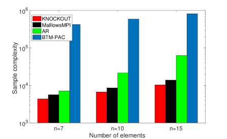
Figure 1: Comparison of sample complexity for several models, and different input sizes , with $\epsilon=0.05$ and $\delta=0.1$

In Figure 1, we compare the sample complexity of algorithms when there are 7, 10 and 15 elements. Our algorithm outperforms all the others. BTM-PAC performs much worse in comparison to others because of high constants in the algorithm. Further BTM-PAC allows comparing an element with itself since the main objective in  Yue & Joachims (2011) is to reduce the regret. We include more comparisons with BTM-PAC in Appendix G. We exclude BTM-PAC for further experiments with higher number of elements.

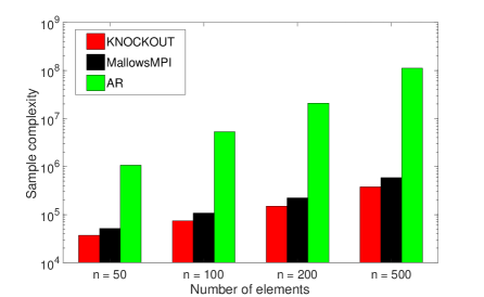
Figure 2: Comparison of sample complexity for large input size, $\epsilon=0.05$, and $\delta=0.1$

In Figure 2, we compare the algorithms when there are 50, 100, 200 and 500 elements. Our algorithm outperforms others for higher number of elements too. Performance of AR gets worse as the number of elements increases since Borda scores of the elements get closer to each other and hence AR takes more comparisons to eliminate an element. Notice that number of comparisons is in logarithmic scale and hence the performance of MallowsMPI appears to be close to that of ours.

As noted in Szörényi et al. (2015), sample complexity of MallowsMPI gets worse as $\tilde{p}(i,j)$ gets close to $0$. To show the pronounced effect, we use the stochastic model $p(1,j)=0.6\ \forall j>1$, $p(i,j)=0.5+\tilde{p}\ \forall j>i,i>1$ where $\tilde{p}<0.1$, and the number of elements is 15. Here too we find $0.05$-maximum with $\delta=0.1$. Note that $i=1$ is the only $0.05$-maximum in this stochastic model.

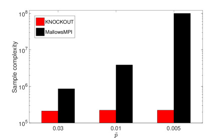
Figure 3: Sample complexity comparison of Knockout with MallowsMPI for different values of $\tilde{p}$, with $\epsilon=0.05$ and $\delta=0.1$

In Figure 3, we compare the algorithms for different values of $\tilde{p}$: 0.01, 0.005 and 0.001. As discussed above, the performance of MallowsMPI gets much worse whereas our algorithm’s performance stays unchanged. The reason is that MallowsMPI finds the Condorcet winner using successive elimination technique and as $\tilde{p}$ gets closer to 0, MallowsMPI takes more comparisons for each elimination. Our algorithm tries to find an alternative which defeats Condorcet winner with probability $\geq 0.5-0.05$ and hence for alternatives that are very close to each other, our algorithm declares either one of them as winner after comparing them for certain number of times.

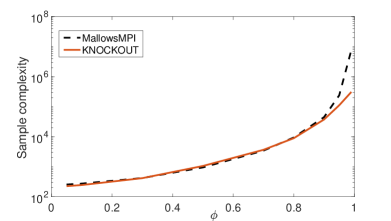
Figure 4: Sample complexity of Knockout and MallowsMPI under Mallows model for various values of $\phi$

Next we evaluate Knockout on Mallows model which does not satisfy triangle inequality. Mallows is a parametric model which is specified by single parameter $\phi$. As in Busa-Fekete et al. (2014a), we consider $n=10$ elements and various values for $\phi$: 0.03, 0.1, 0.3, 0.5, 0.7, 0.8, 0.9, 0.95 and 0.99. Here again we seek to find $0.05$-maximum with $\delta=0.05$. As we can see in Figure 4, sample complexity of Knockout and MallowsMPI is essentially same under small values of $\phi$ but Knockout outperforms MallowsMPI as $\phi$ gets close to $1$ since comparison probabilities grow closer to $1$. Surprisingly, for all values of $\phi$ except for 0.99, Knockout returned Condorcet winner in all runs. For $\phi=0.99$, Knockout returned second best element in 10 runs out of 100. Note that $\tilde{p}(1,2)=0.0025$ and hence Knockout still outputed a $0.05$-maximum. Even though we could not show theoretical guarantees of Knockout under Mallows model, our simulations suggest that it can perform well even under this model.

More experiments are provided in Appendix G.

7 Conclusion

We studied maximum selection and ranking using noisy comparisons for the broad model where the comparison probabilities satisfy strong stochastic transitivity and the triangle inequality. For maximum selection, we presented a simple algorithm with linear, hence optimal, sample complexity. For ranking we presented a framework that improves the performance of many ranking algorithms and applied it to merge ranking to derive a near-optimal ranking algorithm.

We conducted several experiments and showed that our algorithms perform well not only in theory, but also in practice. Furthermore, they out-performed all existing algorithms.

The maximum-selection experiments suggest that our algorithm performs well even without the triangle-inequality assumption. It would be of interest to extend our theoretical guarantees to this case. For ranking, it would be interesting to close the $(\log\log n)^{3}$ ratio between the upper- and lower- complexity bounds.

Appendix A Merge Ranking

We first introduce a subroutine that is used by Merge-Rank. It merges two ordered sets in the presence of noisy comparisons.

A.1 Merge

Merge takes two ordered sets $S_{1}$ and $S_{2}$ and outputs an ordered set $Q$ by merging them. Merge starts by comparing the first elements in each set $S_{1}$ and $S_{2}$ and places the loser in the first position of $Q$. It compares the two elements sufficient times to make sure that output is near-accurate. Then it compares the winner and the element right to loser in the corresponding set. It continues this process until we run out of one of the sets and then adds the remaining elements to the end of $Q$ and outputs $Q$.

Algorithm 6 Merge

Input: Sets $S_{1},S_{2}$, bias $\epsilon$, confidence $\delta$.
Initialize: $i=1$, $j=1$ and $O=\emptyset$.

1. while $i\leq|S_{1}|$ and $j\leq|S_{2}|$.

   1. if $S_{1}(i)=\textsc{Compare}{\left({S_{1}(i),S_{2}(j),\epsilon,\delta}\right)}$, then append $S_{1}(i)$ at the end of $O$ and $i=i+1$.

   2. else append $S_{2}(j)$ at the end of $O$ and $j=j+1$.

2. if $i\leq|S_{1}|$, then append $S_{1}(i:|S_{1}|)$ at the end of $O$.

3. if $j\leq|S_{2}|$, then append $S_{2}(j:|S_{2}|)$ at the end of $O$.

Output: $O$.

We show that when we merge two ordered sets using Merge, the error of resulting ordered set is not high compared to the maximum of errors of individual ordered sets.

Lemma 16.

With probability $\geq 1-(|S_{1}|+|S_{2}|)\delta$, error of $\textsc{Merge}{\left({S_{1},S_{2},\epsilon,\delta}\right)}$ is at most $\epsilon$ more than the maximum of errors of $S_{1}$ and $S_{2}$. Namely, with probability $\geq 1-(|S_{1}|+|S_{2}|)\delta$,

$$err{\left({\textsc{Merge}{\left({S_{1},S_{2},\epsilon,\delta}\right)}}\right)}\leq\max{\left({err(S_{1}),err(S_{2})}\right)}+\epsilon.$$

A.2 Merge-Rank

Now we present the algorithm Merge-Rank. Merge-Rank partitions the input set $S$ into two sets $S_{1}$ and $S_{2}$ each of size $|S|/2$. It then orders $S_{1}$ and $S_{2}$ separately using Merge-Rank and combines the ordered sets using Merge. Notice that Merge-Rank is a recursive algorithm. The singleton sets each containing an unique element in $S$ are merged first. Two singleton sets are merged to form a set with two elements, then the sets with two elements are merged to form a set with four elements and henceforth. By Lemma 16, each merge with bound parameter $\epsilon^{\prime}$ adds at most $\epsilon^{\prime}$ to the error. Since error of singleton sets is $0$ and each element takes part in $\log n$ merges, the error of the output set is at most $\epsilon^{\prime}\log n$. Hence with bound parameter $\epsilon/\log n$, the error of the output set is less than $\epsilon$.

Algorithm 7 Merge-Rank

Input: Set $S$, bias $\epsilon$, confidence $\delta$.

1. $S_{1}=\textsc{Merge-Rank}{\left({S(1:{\lfloor{|S|/2}\rfloor}),\epsilon,\delta}\right)}$.

2. $S_{2}=\textsc{Merge-Rank}{\left({S({\lfloor{|S|/2}\rfloor}+1:|S|),\epsilon,\delta}\right)}$.

Output: $\textsc{Merge}{\left({S_{1},S_{2},\epsilon,\delta}\right)}$.

Appendix B Algorithms for Ranking

Algorithm 8 Interval-Binary-Search

Input: Ordered array $S$, search element $e$, bias $\epsilon$

1. $T$ = Build-Binary-Search-Tree$(|S|)$.

2. Initialize set $Q=\emptyset$, node $\alpha=\text{root}(T)$, and count $c=0$.

3. repeat for $30\log n$ times

   1. if $\alpha_{2}-\alpha_{1}>1$,

      1. Add $\alpha_{1}$, $\alpha_{2}$ and $\left\lceil\frac{\alpha_{1}+\alpha_{2}}{2}\right\rceil$ to $Q$.

      2. if Compare$(S(\alpha_{1}),e,\frac{10}{\epsilon^{2}})>1/2$ or Compare$(e,S(\alpha_{2}),\frac{10}{\epsilon^{2}})>1/2$ then go back to the parent, $\alpha=\text{parent}(\alpha).$

      3. else

         • if Compare$(S(\left\lceil\frac{\alpha_{1}+\alpha_{2}}{2}\right\rceil),e,\frac{10}{\epsilon^{2}})>1/2$ go to the left child,$\alpha=\text{left}(\alpha).$

         • else go to the right child, $\alpha=\text{right}(\alpha).$

   2. else

      1. if Compare$(e,S(\alpha_{1}),\frac{10}{\epsilon^{2}})>1/2$ and Compare$(S(\alpha_{2}),a,\frac{10}{\epsilon^{2}})>1/2$,

         $$c=c+1.$$

      2. else

         1. if $c=0$, $\alpha=\text{parent}(\alpha)$.

         2. else $c=c-1$.

4. 1. if $c>10\log n$, Output: $\alpha_{1}$.

   2. else Output: Binary-Search$(S,Q,e,2\epsilon)$.

Algorithm 9 Build-Binary -Search-Tree

Input: size $n$.
// Recall that each node $m$ in the tree is an interval between left end $m_{1}$ and right end $m_{2}$.

1. Initialize set $T^{\prime}=\emptyset$.

2. Initialize the tree $T$ with the root node $(1,n)$.

   $$m=(1,n)\qquad \text{where }m_{1}=1\text{ and }m_{2}=n,$$

   $$\text{root}(T) =m$$

3. Add $m$ to $T^{\prime}$.

4. while $T^{\prime}$ is not empty

   1. Consider a node $i$ in $T^{\prime}$.

   2. if $i_{2}-i_{1}>1$, create a left child and right child to $i$ and set their parents as $i$.

      $$\alpha={\left({i_{1},\left\lceil\frac{i_{1}+i_{2}}{2}\right\rceil}\right)},\qquad \beta={\left({\left\lceil{\frac{i_{1}+i_{2}}{2}}\right\rceil,i_{2}}\right)},$$

      $$\text{left}(i)=\alpha,\qquad \text{right}(i)=\beta,$$

      $$\text{parent}(\alpha)=i,\qquad \text{parent}(\beta)=i.$$

      and add nodes $\alpha$ and $\beta$ to $T^{\prime}$.

   3. Remove node $i$ from $T^{\prime}$.

Output: $T$.

Algorithm 10 Binary-Search

Input: Ordered array $S$, ordered array $Q$, search item $e$, bias $\epsilon$.
Initialize: $l=1$, $h=|Q|$.

1. while $h-l>0$

   1. $t=$ Comapre${\left({e,S(Q(\left\lceil\frac{l+h}{2}\right\rceil),{\frac{10\log n}{\epsilon^{2}}}}\right)}$.

   2. if $t\in\left[\frac{1}{2}-3\epsilon,\frac{1}{2}+3\epsilon\right]$, then Output: $Q(\left\lceil\frac{l+h}{2}\right\rceil)$.

   3. else if $t<\frac{1}{2}-3\epsilon$, then move to the right.

      $$l=\left\lceil\frac{l+h}{2}\right\rceil.$$

   4. else move to the left.

      $$h=\left\lceil\frac{l+h}{2}\right\rceil.$$

Output: $Q(h)$.

Appendix C Some tools for proving lemmas

We first prove an auxilliary result that we use in the future analysis.

Lemma 17.

Let $W=\textsc{Compare}(i,j,\epsilon,\delta)$ and $L$ be the other element. Then with probability $\geq 1-\delta$,

$$p({W,L})\geq\frac{1}{2}-\epsilon.$$

Proof.

Note that if $|\tilde{p}(i,j)|<\epsilon$, then $p(i,j)>\frac{1}{2}-\epsilon$ and $p(j,i)>\frac{1}{2}-\epsilon$. Hence, $p(W,L)\geq\frac{1}{2}-\epsilon$.

If $|\tilde{p}(i,j)|\geq\epsilon$, without loss of generality, assume that $i$ is a better element i.e., $\tilde{p}(i,j)\geq\epsilon$. By Lemma 1, with probability atleast $1-\delta$, $W=i$. Hence

$$Pr{\left({p(W,L)\geq\frac{1}{2}-\epsilon}\right)}=Pr(W=i)\geq 1-\delta.\qed$$

We now prove a Lemma that follows from strong stochastic transitivity and stochastic triangle inequality that we will use in future analysis.

Lemma 18.

If $\tilde{p}(i,j)\leq\epsilon_{1}$, $\tilde{p}(j,k)\leq\epsilon_{2}$, then $\tilde{p}(i,k)\leq\epsilon_{1}+\epsilon_{2}$.

Proof.

We will divide the proof into four cases based on whether $\tilde{p}(i,j)>0$ and $\tilde{p}(j,k)>0$.

If $\tilde{p}(i,j)\leq 0$ and $\tilde{p}(j,k)\leq 0$, then by strong stochastic transitivity, $\tilde{p}(i,k)\leq 0\leq\epsilon_{1}+\epsilon_{2}$.

If $0<\tilde{p}(i,j)\leq\epsilon_{1}$ and $0<\tilde{p}(j,k)\leq\epsilon_{2}$, then by stochastic traingle inequality, $\tilde{p}(i,k)\leq\epsilon_{1}+\epsilon_{2}$.

If $\tilde{p}(i,j)<0$ and $0<\tilde{p}(j,k)\leq\epsilon_{2}$, then by strong stochastic transitivity, $\tilde{p}(i,k)\leq\epsilon_{2}\leq\epsilon_{1}+\epsilon_{2}$.

If $0<\tilde{p}(i,j)\leq\epsilon_{1}$ and $\tilde{p}(j,k)<0$, then by strong stochastic transitivity, $\tilde{p}(i,k)\leq\epsilon_{1}\leq\epsilon_{1}+\epsilon_{2}$. ∎

Appendix D Proofs of Section 4

Proof of Lemma  1

Proof.

Let $\hat{p}_{i}^{r}$ and $\hat{c}^{r}$ denote $\hat{p}_{i}$ and $\hat{c}$ respectively after $r$ number of comparisons. Output of $\textsc{Compare}(i,j,\epsilon,\delta)$ will not be $i$ only if $\hat{p}_{i}^{r}<\frac{1}{2}+\epsilon-\hat{c}^{r}$ for any $r<m=\frac{1}{2\epsilon^{2}}\log\frac{2}{\delta}$ or if $\hat{p_{i}}<\frac{1}{2}$ for $r=m$. We will show that the probability of each of these events happening is bounded by $\frac{\delta}{2}$. Hence by union bound, Lemma follows.

After $r$ comparisons, by Chernoff bound,

$$Pr(\hat{p}_{i}^{r}<\frac{1}{2}+\epsilon-\hat{c}^{r})\leq e^{-2r(\hat{c}^{r})^{2}}=e^{-\log\frac{4r^{2}}{\delta}}=\frac{\delta}{4r^{2}}.$$

Using union bound,

$$Pr(\exists r\text{ s.t. }\hat{p}_{i}^{r}\leq\frac{1}{2}+\epsilon-\hat{c}^{r})\leq\frac{\delta}{2}$$

After $m=\frac{1}{2\epsilon^{2}}\log\frac{2}{\delta}$ rounds, by Chernoff bound,

$$Pr(\hat{p}_{i}^{m}<\frac{1}{2})\leq e^{-2m\epsilon^{2}}=\frac{\delta}{2}.\qed$$

Proof of Lemma 2

Proof.

Each of the $\frac{|S|}{2}$ pairs is compared at most $\frac{1}{2\epsilon^{2}}\log\frac{2}{\delta}$ times, hence the total comparisons is $\leq\frac{|S|}{4\epsilon^{2}}\log\frac{2}{\delta}$. Let $k^{*}=\text{max}(\textsc{Knockout-Round}(S,\epsilon,\delta))$ and $s^{*}=\text{max}(S)$. Let $a$ be the element paired with $s^{*}$. There are two cases: $\tilde{p}(s^{*},a)\geq\epsilon$ and $\tilde{p}(s^{*},a)<\epsilon$.

If $\tilde{p}(s^{*},a)\geq\epsilon$, by Lemma 1 with probability $\geq 1-\delta$, $s^{*}$ will win and hence by definitions of $s^{*}$ and $k^{*}$, $\tilde{p}(s^{*},k^{*})=0\leq\gamma\epsilon$. Alternatively, if $\tilde{p}(s^{*},a)<\epsilon$, let $\text{winner}(i,j)$ denote the winner between $i$ and $j$ when compared for $\frac{1}{2\epsilon^{2}}\log\frac{1}{\delta}$ times. Then,

$$r(a)\stackrel{{\scriptstyle(a)}}{{\leq}}r(\text{winner}(s^{*},a))\stackrel{{\scriptstyle(b)}}{{\leq}}r(k^{*})\stackrel{{\scriptstyle(c)}}{{\leq}}r(s^{*})$$

where (a) follows from $r(a)\leq r(s^{*})$, (b) and (c) follow from the definitions of $s^{*}$ and $k^{*}$ respectively. From strong stochastic tranisitivity on $a$, $k^{*}$ and $s^{*}$, $\tilde{p}(s^{*},k^{*})\leq\gamma\tilde{p}(s^{*},a)\leq\gamma\epsilon$. ∎

Proof of Theorem 3

Proof.

We first show that with probability $\geq 1-\delta$, the output of Knockout is an $\epsilon$-maximum. Let $\epsilon_{i}=c\epsilon/2^{i/3}$ and $\delta_{i}=\delta/2^{i}$. Note that $\epsilon_{i}$ and $\delta_{i}$ are bias and confidence values used in round $i$. Let $b_{i}$ be a maximum element in the set $S$ before round $i$. Then by Lemma 2, with probability $\geq 1-\delta_{i}$,

$$\tilde{p}(b_{i},b_{i+1})\leq\frac{c\epsilon}{2^{i/3}}.$$ (1)

By union bound, the probability that Equation 1 does not hold for some round $1\leq i\leq\log|S|$ is

$$\leq\sum_{i=1}^{\log|S|}\delta_{i}=\sum_{i=1}^{\log|S|}\frac{\delta}{2^{i}}\leq\delta.$$

With probability $\geq 1-\delta$, Equation 1 holds for all $i$ and by stochastic triangle inequality,

$$\tilde{p}(b_{1},b_{\log{|S|}+1})\leq\sum_{i=1}^{{\log|S|}}\tilde{p}(b_{i},b_{i+1})\leq\sum^{\infty}_{i=1}\frac{c\epsilon}{2^{i/3}}=\epsilon.$$

We now bound the number of comparisons. Let $n_{i}=\frac{|S|}{2^{i-1}}$ be the number of elements in the set at the beginning of round $i$. The number of comparisons at round $i$ is

$$\leq\frac{n_{i}}{2}\cdot\frac{\gamma^{2}2^{2i/3}}{2c^{2}\epsilon^{2}}\cdot\log\frac{2^{i+1}}{\delta}.$$

Hence the number of comparisons in all rounds is

$$\sum^{\log|S|}_{i=1}\frac{|S|}{2^{i}}\cdot\frac{\gamma^{2}2^{2i/3}}{2c^{2}\epsilon^{2}}\cdot\log\frac{2^{i+1}}{\delta} \leq\frac{|S|\gamma^{2}}{2c^{2}\epsilon^{2}}\sum^{\infty}_{i=1}\frac{1}{2^{i/3}}{\left({i+\log\frac{2}{\delta}}\right)}$$

$$=\frac{|S|\gamma^{2}}{2c^{2}\epsilon^{2}}\left(\frac{2^{1/3}}{c^{2}}+\frac{1}{c}\log\frac{2}{\delta}\right)$$

$$={\cal O}{\left({\frac{|S|\gamma^{2}}{\epsilon^{2}}\log\frac{1}{\delta}}\right)}.\qed$$

Appendix E Proofs of Section 5.1

Proof of Lemma 16

Proof.

Let $Q=\textsc{Merge}{\left({S_{1},S_{2},\epsilon,\delta}\right)}$. We will show that for every $k$, w.p. $\geq 1-\delta$, $\tilde{p}(Q(k),Q(l))\leq\max(err(S_{1}),err(S_{2}))+\epsilon$ $\forall l>k$. Note that if this property is true for every element then $err(Q)\leq\max(err(S_{1}),err(S_{2}))+\epsilon$. Since there are $|S_{1}|+|S_{2}|$ elements in the final merged set, the Lemma follows by union bound.

If $S_{1}(i)$ and $S_{2}(j)$ are compared in Merge algorithm, without loss of generality, assume that $S_{1}(i)$ loses i.e., $S_{1}(i)$ appears before $S_{2}(j)$ in $T$. The elements that appear to the right of $S_{1}(i)$ in $Q$ belong to set $Q_{\geq S_{1}(i)}=\{S_{1}(k):k>i\}\bigcup\{S_{2}(k):k\geq j\}$. We will show that w.p. $\geq 1-\delta$, $\forall e\in Q_{\geq S_{1}(i)}$, $\tilde{p}(S_{1}(i),e)\leq\max{\left({err(S_{1}),err(S_{2})}\right)}+\epsilon$.

By definition of error of an ordered set,

$$\tilde{p}(S_{1}(i),S_{1}(k)) \leq err(S_{1})\quad\forall k>i$$ (2)

$$\tilde{p}(S_{2}(j),S_{2}(k)) \leq err(S_{2})\quad\forall k\geq j.$$ (3)

By Lemma 17, w.p. $\geq 1-\delta$,

$$\tilde{p}(S_{1}(i),S_{2}(j))\leq\epsilon.$$ (4)

Hence by Equations 3, 4 and Lemma  18, w.p. $\geq 1-\delta$, $\tilde{p}(S_{1}(i),S_{2}(k))\leq\epsilon+err(S_{2})$ $\forall k\geq j$. ∎

Proof of Lemma 4

Proof.

We first bound the total comparisons. Let $C(Q,\epsilon^{\prime},\delta^{\prime})$ be the number of comparisons that the Merge-Rank uses on a set $Q$. Since Merge-Rank is a recursive algorithm,

$$C(Q,\epsilon^{\prime},\delta^{\prime})\leq C(Q[1:{\lfloor{|Q|/2}\rfloor}],\epsilon^{\prime},\delta^{\prime})$$

$$+C(Q[{\lfloor{|Q|/2}\rfloor}:|Q|],\epsilon^{\prime},\delta^{\prime})+{\frac{|Q|}{2\epsilon^{\prime 2}}\log\frac{2}{\delta^{\prime}}}.$$

From this one can obtain that $C(S,\epsilon^{\prime},\delta^{\prime})={\cal O}{\left({\frac{|S|\log|S|}{\epsilon^{\prime 2}}\log\frac{1}{\delta^{\prime}}}\right)}$. Hence,

$$C{\left({|S|,\frac{\epsilon}{\log|S|},\frac{\delta}{|S|^{2}}}\right)}={\cal O}{\left({\frac{|S|\log^{3}|S|}{\epsilon^{2}}\log\frac{|S|^{2}}{\delta}}\right)}.$$

Now we bound the error. By Lemma 16, with probability $\geq 1-|Q|\delta$,

$$err(\textsc{Merge-Rank}(Q,\epsilon^{\prime},\delta^{\prime}))\leq$$

$$\max\{err{\left({\textsc{Merge-Rank}{\left({Q[1:{\lfloor{|Q|/2}\rfloor}],\epsilon^{\prime},\delta^{\prime}}\right)}}\right)},$$

$$err{\left({\textsc{Merge-Rank}{\left({T[{\lfloor{|Q|/2}\rfloor}+1:|Q|],\epsilon^{\prime},\delta^{\prime}}\right)}}\right)}\}+\epsilon^{\prime}.$$ (5)

We can bound the total times Merge is called in a single instance of $\textsc{Merge-Rank}(S,\epsilon^{\prime},\delta^{\prime})$. Merge combines the singleton sets and forms the sets with two elements, it combines the sets with two elements and forms the sets with four elements and henceforth. Hence the total times Merge is called is $\sum_{i=1}^{\log|S|}\frac{|S|}{2^{i}}\leq|S|.$ Therefore, the probability that Equation E holds every time when two ordered sets are merged in Merge-Rank$(S,\epsilon^{\prime},\delta^{\prime})$ is $\leq|S|\cdot|S|\delta^{\prime}=|S|^{2}\delta^{\prime}.$

If Equation E holds every time Merge is called, then error of Merge-Rank$(S,\epsilon^{\prime},\delta^{\prime})$ is at most $\sum_{i=1}^{\log|S|}\epsilon^{\prime}\leq\epsilon^{\prime}\log|S|$. This is because $err(S)$ is 0 if $S$ has only one element. And a singleton set participates in $\log n$ merges before becoming the final output set.

Therefore, w.p. $\geq 1-|S|^{2}\delta^{\prime}$,

$$err(\textsc{Merge-Rank}(S,\epsilon^{\prime},\delta^{\prime}))\leq\log|S|\epsilon^{\prime}.$$

Hence with probability $\geq 1-\delta$,

$$err{\left({\textsc{Merge-Rank}{\left({S,\frac{\epsilon}{\log|S|},\frac{\delta}{|S|^{2}}}\right)}}\right)}\leq\epsilon.\qed$$

Appendix F Proofs for Section 5.2

Proof of Lemma 5

Proof.

Let set $S$ be ordered s.t. $\tilde{p}(S(i),S(j))\geq 0$ $\forall i>j$. Let $S_{k}^{\prime\prime}=S(k:k+5(\log n)^{x+1}-1)$ The probability that none of the elements in $S_{k}^{\prime\prime}$ is selected for a given $k$ is

$$\leq{\left({1-\frac{5(\log n)^{x+1}}{n}}\right)}^{n/(\log n)^{x}}<\frac{1}{n^{5}}.$$

Therefore by union bound, the probability that none of the elements in $S_{k}^{\prime\prime}$ is selected for any $k$ is

$$\leq n\cdot\frac{1}{n^{5}}=\frac{1}{n^{4}}.\qed$$

Proof of Lemma 7

We prove Lemma 7 by dividing it into further smaller lemmas.

We divide all elements into $S$ into two sets based on distance from anchors. First set contains all elements that are far away from all anchors and the second set contains all elements which are close to atleast one of the anchors. Interval-Binary-Search acts differently on both sets.

We first show that for elements in the first set, Interval-Binary-Search places them in between the right anchors by using just the random walk subroutine.

For elements in the second set, Interval-Binary-Search might fail to find the right anchors just by using the random walk subroutine. But we show that Interval-Binary-Search visits a close anchor during random walk and Binary-Search finds a close anchor from the set of visited anchors using simple binary search.

We first prove Lemma 7 for the elements of first set.

Lemma 19.

For $\epsilon^{\prime\prime}>\epsilon^{\prime}$, consider an $\epsilon^{\prime}$-ranked $S^{\prime}$. If an element $e$ is such that $|\tilde{p}(e,S^{\prime}(j))|>\epsilon^{\prime\prime}$ $\forall j$, then with probability $\geq 1-\frac{1}{n^{6}}$ step  4a of Interval-Binary-Search$(S^{\prime},e,\epsilon^{\prime\prime})$ outputs the index $y$ such that $\tilde{p}(e,S^{\prime}(y))>\epsilon^{\prime\prime}$ and $\tilde{p}(S^{\prime}(y+1),e)>\epsilon^{\prime\prime}$.

Proof.

We first show that there is a unique $y$ s.t. $\tilde{p}(e,S^{\prime}(y))>\epsilon^{\prime\prime}$ and $\tilde{p}(S^{\prime}(y+1),e)>\epsilon^{\prime\prime}$.

Let $i$ be the largest index such that $\tilde{p}(e,S^{\prime}(i))>\epsilon^{\prime\prime}$. By Lemma 18, $\tilde{p}(e,S^{\prime}(j))>\epsilon^{\prime\prime}-\epsilon^{\prime}>0\quad\forall j<i$. Hence by the assumption on $e$, $\tilde{p}(e,S^{\prime}(j))>\epsilon^{\prime\prime}\quad\forall j<i$. Let $k$ be the smallest index such that $\tilde{p}(S^{\prime}(k),e)>\epsilon^{\prime\prime}$. By a similar argument as previously, we can show that $\tilde{p}(S^{\prime}(j),e)>\epsilon^{\prime\prime}\quad\forall j>k$.

Hence by the above arguments and the fact that $|\tilde{p}(e,S^{\prime}(j))|>\epsilon^{\prime\prime}\quad\forall j$, there exists only one $y$ such that $\tilde{p}(e,S^{\prime}(y))>\epsilon^{\prime\prime}$ and $\tilde{p}(S^{\prime}(y+1),e)>\epsilon^{\prime\prime}$.

Thus in the tree $T$, there is only one leaf node $w$ such that $\tilde{p}(e,S^{\prime}(w_{1}))>\epsilon^{\prime\prime}$ and $\tilde{p}(S^{\prime}(w_{2}),e)>\epsilon^{\prime\prime}$.

Consider some node $m$ which is not an ancestor of $w$. Then either $\tilde{p}(S^{\prime}(m_{1}),e)>\epsilon^{\prime\prime}$ or $\tilde{p}(S^{\prime}(m_{2}),e)<-\epsilon^{\prime\prime}$. Since we compare $e$ with $S^{\prime}(m_{l})$ and $S^{\prime}(m_{h})$ $\frac{10}{\epsilon^{\prime\prime 2}}$ times, we move to the parent of $m$ with probability atleast $\frac{19}{20}$.

Consider some node $m$ which is an ancestor of $w$. Then $\tilde{p}(S^{\prime}(m_{l}),e)<-\epsilon^{\prime\prime}$ , $\tilde{p}(S^{\prime}(m_{h}),e)>\epsilon^{\prime\prime}$, and $|\tilde{p}(S^{\prime}(\left\lceil\frac{m_{l}+m_{h}}{2}\right\rceil),e)|>\epsilon^{\prime\prime}$. Therefore we move in direction of $q$ with probability atleast $\frac{19}{20}$.

Therefore if we are not at $q$, then we move towards $q$ with probability atleast $\frac{19}{20}$ and if we are at $q$ then the count $c$ increases with probability atleast $\frac{19}{20}$.

Since we start at most $\log n$ away from $q$ if we move towards $e$ for $21\log n$ then the algorithm will output $y$. The probability that we will have less than $21\log n$ right comparisons is $\leq e^{-30\log nD(\frac{21}{30}||\frac{19}{20})}\leq e^{-30\log nD(\frac{21}{30}||\frac{19}{20})}\leq\frac{1}{n^{6}}$. ∎

To prove Lemma 7 for the elements of the second set, we first show that the random walk subroutine of algorithm Interval-Binary-Search placing an element in wrong bin is highly unlikely.

Lemma 20.

For $\epsilon^{\prime\prime}>\epsilon^{\prime}$, consider an $\epsilon^{\prime}$-ranked set $S^{\prime}$. Now consider an element $e$ and $y$ such that either $\tilde{p}(S^{\prime}(y),e)>\epsilon^{\prime\prime}$ or $\tilde{p}(S^{\prime}(y+1),e)<-\epsilon^{\prime\prime}$, then step  4a of Interval-Binary-Search$(S^{\prime},e,\epsilon^{\prime\prime})$ will not output $y$ with probability $\geq 1-\frac{1}{n^{7}}$.

Proof.

Recall that step  4a of Interval-Binary-Search outputs $y$ if we are at the leaf node $(y,y+1)$ and the count $c$ is atleast $10\log n$.

Since either $\tilde{p}(S^{\prime}(y),e)>\epsilon^{\prime\prime}$ or $\tilde{p}(S^{\prime}(y+1),e)<-\epsilon^{\prime\prime}$, when we are at leaf node $(y,y+1)$, the count decreases with probability atleast $\frac{19}{20}$. Hence the probability that Interval-Binary-Search is at (y,y+1) and the count is greater than $10\log n$ is at most $\sum_{i=10\log n}^{30\log n}e^{-i\cdot D(\frac{i-10\log n}{2i}||\frac{19}{20})}<10\log ne^{-10\log nD(\frac{1}{3}||\frac{19}{20})}\leq\frac{1}{n^{7}}$. ∎

We now show that for an element of the second set, the random walk subroutine either places it in correct bin or visits a close anchor.

Lemma 21.

For $\epsilon^{\prime\prime}>\epsilon^{\prime}$, consider an $\epsilon^{\prime}$-ranked set $S^{\prime}$. Now consider an element $e$ that is close to an element in $S^{\prime}$ i.e., $\exists g:|\tilde{p}(S^{\prime}(g),e)|<\epsilon^{\prime\prime}$. Step  4a of Interval-Binary-Search$(S^{\prime},e,\epsilon^{\prime\prime})$ will either output the right index $y$ such that $\tilde{p}(S^{\prime}(y),e)<\epsilon^{\prime\prime}$ and $\tilde{p}(S^{\prime}(y+1),e)>-\epsilon^{\prime\prime}$ or Interval-Binary-Search visits $S^{\prime}(h)$ such that $|\tilde{p}(S^{\prime}(h),e)|<2\epsilon^{\prime\prime}$ with probability$\geq 1-\frac{1}{n^{6}}$.

Proof.

By Lemma 20, step  4a of Interval-Binary-Search does not output a wrong interval with probability $1-\frac{1}{n^{7}}$. Hence we just need to show that w.h.p., $e$ visits a close anchor.

Let $i$ be the largest index such that $\tilde{p}(e,S^{\prime}(i))>2\epsilon^{\prime\prime}$. Then $\forall k<i$, by Lemma 18, $\tilde{p}(e,S(k))>2\epsilon^{\prime\prime}-\epsilon^{\prime}>\epsilon^{\prime\prime}$ .

Let $j$ be the smallest index such that $\tilde{p}(S^{\prime}(j),e)>2\epsilon^{\prime\prime}$. Then $\forall k>j$, by Lemma 18, $\tilde{p}(S^{\prime}(k),e)>\epsilon^{\prime\prime}$ .

Therefore for $u<v$ such that $\min(|\tilde{p}(S^{\prime}(u),e)|,|\tilde{p}(S^{\prime}(v),e)|)\geq 2\epsilon^{\prime\prime}$ only one of three sets $\{x:x<u\}$,$\{x:u<x<v\}$ and $\{x:x>v\}$ contains an index $z$ such that $|\tilde{p}(S^{\prime}(z),e)|<\epsilon^{\prime\prime}$.

Let a node $\alpha$ be s.t. for some $c\in\{\alpha_{1},\alpha_{2},{\lceil{\frac{\alpha_{1}+\alpha_{2}}{2}}\rceil}\}$, $|\tilde{p}(S^{\prime}(c),e)|\leq 2\epsilon^{\prime\prime}$. If Interval-Binary-Search reaches such a node $\alpha$ then we are done.

So assume that Interval-Binary-Search is at a node $\beta$ s.t. $\forall c\in\{\beta_{1},\beta_{2},{\lceil{\frac{\beta_{1}+\beta_{2}}{2}}\rceil}\}$, $|\tilde{p}(S^{\prime}(c),e)|>2\epsilon^{\prime\prime}$. Note that only one of three sets $\{x:x<\beta_{1}\text{ or }x>\beta_{2}\}$, $\{x:\beta_{1}<x<{\lceil{\frac{\beta_{1}+\beta_{2}}{2}}\rceil}\}$ and $\{x:{\lceil{\frac{\beta_{1}+\beta_{2}}{2}}\rceil}<x<\beta_{2}\}$ contains an index $z$ such that $|\tilde{p}(S^{\prime}(z),e)|<\epsilon^{\prime\prime}$ and Interval-Binary-Search moves towards that set with probability $\frac{19}{20}$. Hence the probability that we never visit an anchor that is less than $2\epsilon^{\prime\prime}$ away is at most $e^{-30\log nD(\frac{1}{2}||\frac{19}{20})}\leq\frac{1}{n^{7}}$. ∎

We now complete the proof by showing that for an element $e$ from the second set, if $Q$ contains an index $y$ of an anchor that is close to $e$, Binary-Search will output one such index.

Lemma 22.

For $\epsilon^{\prime\prime}>\epsilon^{\prime}$, consider ordered sets $S^{\prime},Q$ s.t. $p(S^{\prime}(Q(i)),S^{\prime}(Q(j)))>\frac{1}{2}-\epsilon^{\prime}$ $\forall i>j$. For an element $e$ s.t., $\exists g:|\tilde{p}(S^{\prime}(Q(g)),a)|<2\epsilon^{\prime\prime}$, Binary-Search$(S^{\prime},Q,a,\epsilon^{\prime\prime})$ will return $y$ such that $|\tilde{p}(S^{\prime}(Q(y)),a)|<4\epsilon^{\prime\prime}$ with probability $\geq 1-\frac{1}{n^{6}}$.

Proof.

At any stage of Binary-Search, there are three possibilities that can happen . Consider the case when we are comparing $e$ with $S^{\prime}(Q(i))$.

1. $|\tilde{p}(S^{\prime}(Q(i)),e)<2\epsilon^{\prime\prime}|$. Probability that the fraction of wins for $e$ is not between $\frac{1}{2}-3\epsilon^{\prime\prime}$ and $\frac{1}{2}+3\epsilon^{\prime\prime}$ is less than $e^{-\frac{10\log n}{\epsilon^{\prime\prime 2}}\epsilon^{\prime\prime 2}}\leq\frac{1}{n^{10}}$. Hence Binary-Search outputs $Q(i)$.

2. $\tilde{p}(S^{\prime}(Q(i)),e)>2\epsilon^{\prime\prime}$. Probability that the fraction of wins for $e$ is more than $\frac{1}{2}$ is less than $e^{-\frac{10\log n}{\epsilon^{\prime\prime 2}}\epsilon^{\prime\prime 2}}\leq\frac{1}{n^{1}0}$. So Binary-Search will not move right. Also notice that $\tilde{p}(S^{\prime}(Q(j)),e)>2\epsilon^{\prime\prime}-\epsilon^{\prime}>\epsilon^{\prime\prime}$ $\forall j>i$.

3. $\tilde{p}(S^{\prime}(Q(i)),e)>4\epsilon^{\prime\prime}$. Probability that the fraction of wins for $e$ is more than $\frac{1}{2}-3\epsilon^{\prime\prime}$ is less than $e^{-\frac{10\log n}{\epsilon^{\prime\prime 2}}\epsilon^{\prime\prime 2}}\leq\frac{1}{n^{10}}$. Hence Binary-Search will move left. Also notice that $\tilde{p}(S^{\prime}(Q(j)),e)>4\epsilon^{\prime\prime}-\epsilon^{\prime}>\epsilon^{\prime\prime}$ $\forall j>i$.

We can show similar results for $\tilde{p}(S^{\prime}(Q(i)),e)<-2\epsilon^{\prime\prime}$ and $\tilde{p}(S^{\prime}(Q(i)),e)<-4\epsilon^{\prime\prime}$. Hence if $|\tilde{p}(S^{\prime}(Q(i)),e)|<2\epsilon^{\prime\prime}$ then Binary-Search outputs $Q(i)$, and if $2\epsilon^{\prime\prime}<|\tilde{p}(S^{\prime}(Q(i)),e)|<4\epsilon^{\prime\prime}$ then either Binary-Search outputs $Q(i)$ or moves in the correct direction and if $|\tilde{p}(S^{\prime}(Q(i)),e)|>4\epsilon^{\prime\prime}$, then Binary-Search moves in the correct direction. ∎

Lemma 23.

Interval-Binary-Search$(S,e,\epsilon)$ terminates in ${\cal O}(\frac{\log n\log\log n}{\epsilon^{2}})$ comparisons for any set $S$ of size $O(n)$.

Proof.

Step 3 of Interval-Binary-Search runs for 30 $\log n$ iterations. In each iteration, Interval-Binary-Search compares $e$ with at most 3 anchors and repeats each comparison for $10/\epsilon^{2}$. So total comparisons in step $3$ is ${\cal O}(\log n/\epsilon^{2})$. The size of $Q$ is upper bounded by $90\log n$ and Binary-Search does a simple binary search over $Q$ by repeating each comparison $10\log n/\epsilon^{2}$. Hence total comparisons used by Binary-Search is ${\cal O}(\log n\log\log n/\epsilon^{2})$ ∎

Combining Lemmas  6, 20, 21, 22, 23 yields the result.

Proof of Lemma 10

Proof.

Combining Lemmas  6, 9 and using union bound, at the end of step  5a ,w.p. $\geq 1-\frac{2}{n^{3}}$, $S^{\prime}$ is $\epsilon^{\prime}$-ranked and $\forall j,e\in B_{j}$, $\min(\tilde{p}(e,S^{\prime}(j)),\tilde{p}(S^{\prime}(j+1),e))>5\epsilon^{\prime\prime}$. Hence by Lemma 18, $\forall j,k<j,e\in B_{j}$, $\tilde{p}(e,S^{\prime}(k))>5\epsilon^{\prime\prime}-\epsilon^{\prime}>4\epsilon^{\prime\prime}$. Similarly, $\forall j,k>j,e\in B_{j}$, $\tilde{p}(S^{\prime}(k),e)>5\epsilon^{\prime\prime}-\epsilon^{\prime}>4\epsilon^{\prime\prime}$.

If $|B_{j}|>0$, then $\tilde{p}(e,S^{\prime}(k))>4\epsilon^{\prime\prime}$ for $e\in B_{j},k\leq j$, $\tilde{p}(S^{\prime}(l),e)>4\epsilon^{\prime\prime}$ for $e\in B_{j},l\geq j$. Hence by strong stochastic transitivity, $\tilde{p}(S^{\prime}(l),S^{\prime}(k))>4\epsilon^{\prime\prime}$ for $l\geq j\geq k$. Therefore there exists $k,l$ s.t. $\tilde{p}(S^{\prime}(l),f)>0$ $\forall f\in\{S^{\prime}(y):y\leq j\}$, $\tilde{p}(S^{\prime}(k),S^{\prime}(l))>0$ and $\tilde{p}(f,S^{\prime}(k))>0$ $\forall f\in\{S^{\prime}(y):y\geq j\}$. Now by Lemma  5, w.p. $\geq 1-\frac{1}{n^{3}}$, size of such set $B_{j}$ is less than $10(\log n)^{x+1}$.

Lemma follows by union bound. ∎

Proof of Theorem 12

We first bound the running time of Binary-Search-Ranking algorithm.

Theorem 24.

Binary-Search-Ranking terminates after $O(\frac{n(\log\log n)^{x}}{\epsilon^{2}}\log n)$ comparisons with probability $\geq 1-\frac{1}{n^{2}}$.

Proof.

Step 2 Rank-$x$ $(S^{\prime},\epsilon^{\prime},\frac{1}{n^{6}})$ terminates after ${\cal O}(\frac{n}{\epsilon^{2}}\log n)$ comparisons with probability $\geq 1-\frac{1}{n^{6}}$.

By Lemma  7, for each element $e$, the step 4a Interval-Binary-Search$(S^{\prime},e,\epsilon^{\prime\prime})$ terminates after ${\cal O}(\frac{\log n\log\log n}{\epsilon^{2}}\log\log n)$ comparisons. Hence step 4 takes at most ${\cal O}(\frac{n\log n\log\log n}{\epsilon^{2}})$ comparisons.

Comparing each element with the anchors in steps 5a takes at most $O(\frac{\log n}{\epsilon^{2}})$ comparisons.

With probability $\geq 1-\frac{1}{n^{4}}$ step 5b Sort-x$(B_{i},\ \epsilon^{\prime\prime},\frac{1}{n^{4}})$ terminates after ${\cal O}(|B_{i}|\frac{(\log|B_{i}|)^{x}}{\epsilon^{2}}\log n)$ comparisons. By Lemma  10, $|B_{i}|\leq 10(\log n)^{x+1}$ for all $i$ w.p. $\geq 1-\frac{3}{n^{3}}$. Hence, w.p. $\geq 1-\frac{3}{n^{3}}$, total comparisons to rank all $B_{i}$s is at most $\sum_{i}{\cal O}(|B_{i}|\frac{(\log|B_{i}|)^{x}}{\epsilon^{2}}\log n)\leq\sum_{i}{\cal O}(\frac{|B_{i}|\ logn(\log(10\log n)^{x+1})^{x}}{\epsilon^{2}})={\cal O}(\frac{n\log n(\log\log n)^{x}}{\epsilon^{2}}).$

Therefore, by summing comparisons over all steps, with probability $\geq 1-\frac{1}{n^{2}}$ total comparisons is at most $O{\left({\frac{n\log n(\log\log n)^{x}}{\epsilon^{2}}}\right)}$. ∎

Now we show that Binary-Search-Ranking outputs an $\epsilon$-ranking with high probability.

Theorem 25.

Binary-Search-Ranking produces an $\epsilon$-ranking with probability at least $1-\frac{1}{n^{2}}$.

Proof.

By combining Lemmas 6, 8, 9, 11 and using union bound, w.p. $\geq 1-\frac{1}{n^{2}}$, at the end of step 5b,

• $S^{\prime}$ is $\epsilon^{\prime}$-

• Each $C_{i}$ has elements such that $|\tilde{p}(C_{i}(j),S(i))|<7\epsilon^{\prime\prime}$ for all $j$.

• Each $B_{i}$ has elements such that $\tilde{p}(S^{\prime}(i),B_{i}(j))<-5\epsilon^{\prime\prime}$ and $\tilde{p}(S^{\prime}(i+1),B_{i}(j))>5\epsilon^{\prime\prime}$.

• All $B_{i}$s are $\epsilon^{\prime\prime}$-ranked.

For $j\geq i$, $e\in B_{j-1}\bigcup{S^{\prime}(j)}\bigcup C_{j}$, $f\in{S^{\prime}(k)}\bigcup C_{k}\bigcup B_{k}$, $\tilde{p}(e,f)\leq\tilde{p}(e,S^{\prime}(i))+\tilde{p}(S^{\prime}(i),S^{\prime}(j))+\tilde{p}(S^{\prime}(j),f)\leq 7\epsilon^{\prime\prime}+\epsilon^{\prime}+7\epsilon^{\prime\prime}<15\epsilon^{\prime\prime}=\epsilon.$ Combining the above result with the fact that all $B_{i}$s are $\epsilon^{\prime\prime}$-ranked proves the Lemma. ∎

Combining Theorems  24, 25 yields the result.

Proof Sketch for Theorem 15

Proof sketch.

Consider a stochastic model where there is an inherent ranking $r$ and for any two consecutive elements $p(i,i+1)=\frac{1}{2}-2\epsilon$. Suppose there is a genie that knows the true ranking $r$ up to the sets ${\left\{r(2i-1),r(2i)\right\}}$ for all $i$ i.e., for each $i$, genie knows $\{r(2i-1),r(2i)\}$ but it does not know the ranking between these two elements. Since consecutive elements have $\epsilon(i,i+1)=2\epsilon>\epsilon$, to find an $\epsilon$-ranking, the genie has to correctly identify the ranking within all the $n/2$ pairs. Using Fano’s inequality from information theory, it can be shown that the genie needs at least $\Omega{\left({\frac{n}{\epsilon^{2}}\log\frac{n}{\delta}}\right)}$ comparisons to identify the ranking of the consecutive elements with probability $1-\delta$. ∎

Appendix G Additional Experiments

As we mentioned in Section 6, BTM-PAC allows comparison of an element with itself. It is not beneficial when the goal is to find $\epsilon$-maximum. So we modify their algorithm by not allowing such comparisons. We refer to this restricted version as R-BTM-PAC.

As seen in figure, performance of BTM-PAC does not increase by much by restricting the comparisons.

We further reduce the constants in R-BTM-PAC. We change Equations (7) and (8) in Yue & Joachims [2011] to $c_{\delta}(t)=\sqrt{\frac{1}{t}\log\frac{n^{3}N}{\delta}}$ and $N={\lceil{\frac{1}{\epsilon^{2}}\log\frac{n^{3}N}{\delta}}\rceil}$, respectively.

We believe the same guarantees hold even with the updated constants. We refer to this improved restricted version as IR-BTM-PAC. Here too we consider the stochastic model where $p(i,j)=0.6\forall\ i<j$ and we find $0.05$-maximum with error probability $\delta=0.1$.

In Figure 5 we compare the performance of Knockout and all variations of BTM-PAC. As the figure suggests, the performance of IR-BTM-PAC improves a lot but Knockout still outperforms it significantly.

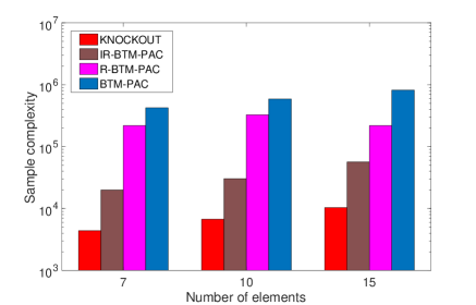
Figure 5: Sample complexity comparison of Knockout and variations of BTM-PAC for different input sizes, with $\epsilon=0.05$ and $\delta=0.1$

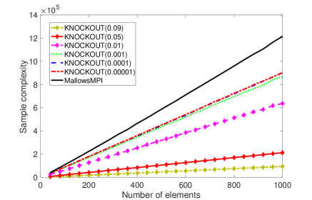
Figure 6: Sample complexity of Knockout for different values of $n$ and $\epsilon$

In Figure 6, we consider the stochastic model where $p(i,j)=0.6\ \forall i<j$ and find $\epsilon$-maximum for different values of $\epsilon$. Similar to previous experiments, we use $\delta=0.1$. As we can see the number of comparisons increases almost linearly with $n$. Further the number of comparisons does not increase significantly even when $\epsilon$ decreases. Also the number of comparisons seem to be converging as $\epsilon$ goes to 0. Knockout outperforms MallowsMPI even for the very small $\epsilon$ values. We attribute this to the subroutine Compare that finds the winner faster when the distance between elements are much larger than $\epsilon$.

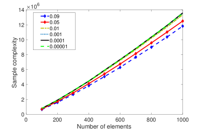
Figure 7: Sample complexity of Merge-Rank for $\epsilon$

For the stochastic model $p(i,j)=0.6\ \forall i<j$, we run our Merge-Rank algorithm to find $0.05$ ranking with $\delta=0.1$. Figure 7 shows that sample complexity does not increase a lot with decreasing $\epsilon$.

References

- Acharya et al. [2014a] Acharya, Jayadev, Jafarpour, Ashkan, Orlitsky, Alon, and Suresh, Ananda Theertha. Sorting with adversarial comparators and application to density estimation. In ISIT, pp. 1682–1686. IEEE, 2014a.
- Acharya et al. [2014b] Acharya, Jayadev, Jafarpour, Ashkan, Orlitsky, Alon, and Suresh, Ananda Theertha. Near-optimal-sample estimators for spherical gaussian mixtures. NIPS, 2014b.
- Acharya et al. [2016] Acharya, Jayadev, Falahatgar, Moein, Jafarpour, Ashkan, Orlitsky, Alon, and Suresh, Ananda Theertha. Maximum selection and sorting with adversarial comparators and an application to density estimation. arXiv preprint arXiv:1606.02786, 2016.
- Ajtai et al. [2015] Ajtai, Miklós, Feldman, Vitaly, Hassidim, Avinatan, and Nelson, Jelani. Sorting and selection with imprecise comparisons. ACM Transactions on Algorithms (TALG), 12(2):19, 2015.
- Braverman & Mossel [2008] Braverman, Mark and Mossel, Elchanan. Noisy sorting without resampling. In Proceedings of the nineteenth annual ACM-SIAM SODA, pp. 268–276. Society for Industrial and Applied Mathematics, 2008.
- Braverman & Mossel [2009] Braverman, Mark and Mossel, Elchanan. Sorting from noisy information. arXiv preprint arXiv:0910.1191, 2009.
- Busa-Fekete et al. [2013] Busa-Fekete, Róbert, Szorenyi, Balazs, Cheng, Weiwei, Weng, Paul, and Hüllermeier, Eyke. Top-k selection based on adaptive sampling of noisy preferences. In Proc. of The ICML, pp. 1094–1102, 2013.
- Busa-Fekete et al. [2014a] Busa-Fekete, Róbert, Hüllermeier, Eyke, and Szörényi, Balázs. Preference-based rank elicitation using statistical models: The case of mallows. In Proc. of the ICML, pp. 1071–1079, 2014a.
- Busa-Fekete et al. [2014b] Busa-Fekete, Róbert, Szörényi, Balázs, and Hüllermeier, Eyke. Pac rank elicitation through adaptive sampling of stochastic pairwise preferences. In AAAI, 2014b.
- Feige et al. [1994] Feige, Uriel, Raghavan, Prabhakar, Peleg, David, and Upfal, Eli. Computing with noisy information. SIAM Journal on Computing, 23(5):1001–1018, 1994.
- Heckel et al. [2016] Heckel, Reinhard, Shah, Nihar B, Ramchandran, Kannan, and Wainwright, Martin J. Active ranking from pairwise comparisons and when parametric assumptions don’t help. arXiv preprint arXiv:1606.08842, 2016.
- Herbrich et al. [2006] Herbrich, Ralf, Minka, Tom, and Graepel, Thore. Trueskill™: a bayesian skill rating system. In Proceedings of the 19th International Conference on Neural Information Processing Systems, pp. 569–576. MIT Press, 2006.
- Jang et al. [2016] Jang, Minje, Kim, Sunghyun, Suh, Changho, and Oh, Sewoong. Top- ranking from pairwise comparisons: When spectral ranking is optimal. arXiv preprint arXiv:1603.04153, 2016.
- Luce [2005] Luce, R Duncan. Individual choice behavior: A theoretical analysis. Courier Corporation, 2005.
- Mukherjee [2011] Mukherjee, Sudipta. Data structures using C : 1000 problems and solutions. 2011.
- Negahban et al. [2012] Negahban, Sahand, Oh, Sewoong, and Shah, Devavrat. Iterative ranking from pair-wise comparisons. In NIPS, pp. 2474–2482, 2012.
- Negahban et al. [2016] Negahban, Sahand, Oh, Sewoong, and Shah, Devavrat. Rank centrality: Ranking from pairwise comparisons. Operations Research, 2016.
- Plackett [1975] Plackett, Robin L. The analysis of permutations. Applied Statistics, pp. 193–202, 1975.
- Radlinski & Joachims [2007] Radlinski, Filip and Joachims, Thorsten. Active exploration for learning rankings from clickthrough data. In Proceedings of the 13th ACM SIGKDD, pp. 570–579. ACM, 2007.
- Radlinski et al. [2008] Radlinski, Filip, Kurup, Madhu, and Joachims, Thorsten. How does clickthrough data reflect retrieval quality? In Proceedings of the 17th ACM conference on Information and knowledge management, pp. 43–52. ACM, 2008.
- Rajkumar & Agarwal [2014] Rajkumar, Arun and Agarwal, Shivani. A statistical convergence perspective of algorithms for rank aggregation from pairwise data. In Proc. of the ICML, pp. 118–126, 2014.
- Syrgkanis et al. [2016] Syrgkanis, Vasilis, Krishnamurthy, Akshay, and Schapire, Robert E. Efficient algorithms for adversarial contextual learning. arXiv preprint arXiv:1602.02454, 2016.
- Szörényi et al. [2015] Szörényi, Balázs, Busa-Fekete, Róbert, Paul, Adil, and Hüllermeier, Eyke. Online rank elicitation for plackett-luce: A dueling bandits approach. In NIPS, pp. 604–612, 2015.
- Urvoy et al. [2013] Urvoy, Tanguy, Clerot, Fabrice, Féraud, Raphael, and Naamane, Sami. Generic exploration and k-armed voting bandits. In Proc. of the ICML, pp. 91–99, 2013.
- Yue & Joachims [2011] Yue, Yisong and Joachims, Thorsten. Beat the mean bandit. In Proc. of the ICML, pp. 241–248, 2011.
- Yue et al. [2012] Yue, Yisong, Broder, Josef, Kleinberg, Robert, and Joachims, Thorsten. The k-armed dueling bandits problem. Journal of Computer and System Sciences, 78(5):1538–1556, 2012.