Efficient adiabatic hydrodynamical simulations of the high-redshift intergalactic medium

Abstract

We present a post-processing tool for gadget-2 adiabatic simulations to model various observed properties of the  Ly$\alpha$ forest at $2.5\leq z\leq 4$ that enables an efficient parameter estimation. In particular, we model the thermal and ionization histories that are not computed self-consistently by default in gadget-2. We capture the effect of pressure smoothing by running gadget-2 at an elevated temperature floor and using an appropriate smoothing kernel. We validate our procedure by comparing different statistics derived from our method with those derived using self-consistent simulations with gadget-3. These statistics are: line of sight density field power spectrum, flux probability distribution function, flux power spectrum, wavelet statistics, curvature statistics, Hi column density (${\rm N_{HI}}$) distribution function, linewidth ($b$) distribution and $b$ versus  $\log{\rm N_{HI}}$ scatter. For the temperature floor of $10^{4}$ K and typical signal-to-noise of 25, the results agree well within 20 percent of the self-consistent gadget-3 simulation. However, this difference is smaller than the expected $1\sigma$ sample variance for an absorption path length of $\sim 5.35$ at $z=3$. Moreover for a given cosmology, we gain a factor of $\sim N$ in computing time for modelling the intergalactic medium under $N\gg 1$ different thermal histories. In addition, our method allows us to simulate the non-equilibrium evolution of thermal and ionization state of the gas and include heating due to non-standard sources like cosmic rays and high energy $\gamma$-rays from Blazars.

1 Introduction

The  Ly$\alpha$ forest seen in the spectra of distant background QSOs trace the distribution of neutral hydrogen (Hi) in the universe at mildly non-linear overdensities ($\Delta\lesssim 10$, Miralda-Escudé et al., 1996; Bi & Davidsen, 1997; Croft et al., 1997). Observed properties of the  Ly$\alpha$ forest are sensitive to fluctuations in the cosmic density and velocity fields and physical conditions like the temperature, turbulence and ionizing radiation prevailing in the intergalactic medium (IGM; Cen et al., 1994; Zhang et al., 1995; Miralda-Escudé et al., 1996; Hernquist et al., 1996). As a result,  Ly$\alpha$ forest has been used in the literature to constrain cosmological parameters such as $\Omega_{\rm m}$, $\Omega_{\rm b}$, $\sigma_{\rm 8}$, $n_{\rm s}$ (see, e.g., Viel et al., 2004a, b; McDonald et al., 2005), the neutrino mass (Palanque-Delabrouille et al., 2015a, b; Yeche et al., 2017), mass of warm dark matter particles (Narayanan et al., 2000; Viel et al., 2005, 2013a) and astrophysical parameters such as the IGM temperature $T_{0}$ at cosmic mean density and slope $\gamma$ of the temperature ($T$) - density ($\Delta$) relation ($T=T_{0}\Delta^{\gamma-1}$, hereafter TDR; Schaye et al., 1999, 2000; Zaldarriaga et al., 2001; McDonald et al., 2001; Theuns & Zaroubi, 2000; Lidz et al., 2010; Becker et al., 2011; Boera et al., 2014) and H i photo-ionization rate ($\Gamma_{\rm HI}$, Rauch et al., 1997; Cooke et al., 1997; Meiksin & White, 2004; Becker & Bolton, 2013; Kollmeier et al., 2014; Shull et al., 2015; Gaikwad et al., 2017a, b; Viel et al., 2016; Gurvich et al., 2017).

Usually constraining these parameters involves comparing different properties of the  Ly$\alpha$ forest derived from observed spectra with those from the simulated ones. Early simulations of  Ly$\alpha$ forest based on lognormal (Bi et al., 1992; Bi & Davidsen, 1997; Gnedin & Hui, 1996; Choudhury et al., 2001) or the Zel’dovich approximation (Doroshkevich & Shandarin, 1977; McGill, 1990), although fast and capture the basic picture, failed to reproduce the quasi- and non-linear density fields accurately (Viel et al., 2002) or washed out the small scale structures in the  Ly$\alpha$ forest (Gnedin & Hui, 1998).

By using cosmological $N$-body simulations (Hernquist & Katz, 1989; Springel, 2005; O’Shea et al., 2005), the  Ly$\alpha$ forest has been modelled in the past using (i) dark matter only simulations where baryons are assumed to follow the dark matter, and the temperature is assigned to the baryons assuming a power-law TDR (Muecket et al., 1996), (ii) smoothed particle hydrodynamic (SPH) codes (Cen et al., 1994; Zhang et al., 1995; Hernquist et al., 1996; Theuns et al., 1998; Davé et al., 1999; Viel et al., 2004a) like gadget-2 and gadget-3 (Springel et al., 2001; Springel, 2005; Bolton et al., 2006), (iii) grid based adaptive mesh refinement (AMR) code enzo (Smith et al., 2011; Shull et al., 2012; Bryan et al., 2014) and (iv) hybrid methods such as  Ly$\alpha$ Mass Association Scheme (LyMAS) in which moderate resolution dark matter only simulation is used after the calibration using high resolution but small volume hydrodynamic simulations (Peirani et al., 2014; Sorini et al., 2016). The main drawback of the dark matter only simulations is that it does not account for the smoothing of the baryonic density field due to finite pressure of the baryons, while these effects are self-consistently accounted for in the SPH and AMR based simulations. Interestingly, the  Ly$\alpha$ forest flux statistics from SPH and AMR simulations are shown to agree with each other to within 10 per cent accuracy (Regan et al., 2007). These simulations can, in principle, incorporate different complex astrophysical processes such as the radiative heating, cooling, shocks, starbursts and AGN induced feedback processes (Kollmeier et al., 2006; McDonald et al., 2006; Davé et al., 2010; Schaye et al., 2010; Viel et al., 2013b).

While the current state of the art hydrodynamical simulations are extremely useful for probing the physical properties of the IGM, the computational expenses severely limit their usage for constraining the unknown model parameters and their associated errors. Various approaches have been introduced to keep the computational expense within manageable limits while exploring the large parameter space. For example, Viel & Haehnelt (2006); Viel et al. (2009) begin by choosing a “best-guess” model and expand the statistical quantities under consideration (e.g., the flux power spectrum) in a Taylor series around this model. Their method requires calculating a limited number of derivatives which can be achieved by running only a few simulations around the best-guess model. The method of McDonald et al. (2005) involves running simulations on a carefully chosen grid in the parameter space and then interpolating between these runs. Other methods include deriving scaling relations between different parameters from a limited number of hydrodynamical simulations which are useful for studying parameter degeneracies (Bolton et al., 2005; Bolton & Haehnelt, 2007; Faucher-Giguère et al., 2008). Since many of the parameters, particularly those related to the thermal state of the IGM, are poorly understood, obtaining robust constraints would require exploring a sufficiently wide range of parameter values. It is thus useful to develop newer methods of simulating the high-$z$ IGM that are efficient, flexible and at the same time sufficiently accurate. This forms one of the main motivation of this work.

In Gaikwad et al. (2017a), we have developed a “Code for Ionization and Temperature Evolution” (cite) to estimate the temperature of the SPH particles in the post-processing step of gadget-2 by taking care of radiative cooling and heating effects. cite allowed us to place good constraints on $\Gamma_{\rm HI}$ while efficiently exploring different thermal histories at low-$z$ ($z\leq 0.5$). While cite works well for the low resolution simulation (gas particle mass $\delta m=1.26\times 10^{7}\>h^{-1}\>{\rm M}_{\sun}$ and pixel size $\delta x=48.8h^{-1}$ ckpc) as shown in Gaikwad et al. (2017a), the dynamical evolution of SPH particles at finite pressure is an important effect when we consider high resolution simulations (e.g. gas particle mass $\delta_{m}=1.01\times 10^{5}\>{\rm M}_{\sun}$ and pixel size $\delta x=9.77h^{-1}$ ckpc). In this article, we present a method to account for this effect by smoothing (in 3 dimensions) the density and velocity fields over a local Jeans scale. We explore the consistency of our method with that from gadget-3 (Springel, 2005, in which the thermal effects on the hydrodynamical evolution of baryonic particles are taken care of in a self-consistent manner) by comparing different  Ly$\alpha$ flux statistics frequently used in the literature. Our method (though approximate) is computationally less expensive and accurate enough to constrain physical parameters through a detailed exploration of possible parameter space. Our code is also flexible enough to incorporate effects such as non-equilibrium evolution of the ionization state of the gas and heating by non-standard sources like Blazars or cosmic rays etc.

This paper is organized as follows. In §2, we describe the gadget-2 and gadget-3 simulations used in this study. We discuss the method of simulating  Ly$\alpha$ forest in §3. We show the consistency of our method with gadget-3 by comparing 8 different statistics in §4. We summarize our results in §5. We use flat $\Lambda$CDM cosmology with parameters $(\Omega_{\Lambda},\Omega_{\rm m},\Omega_{\rm b},h,n_{s},\sigma_{8},Y)\equiv(0.69,0.31,0.0486,0.674,0.96,0.83,0.24)$ consistent with Planck Collaboration et al. (2016). The Hi photoionization rate ($\Gamma_{\rm HI}$) expressed in units of $10^{-12}\>{\rm s}^{-1}$ is denoted as $\Gamma_{\rm 12}$. Unless mentioned all the distances are expressed in comoving co-ordinates.

2 Simulation

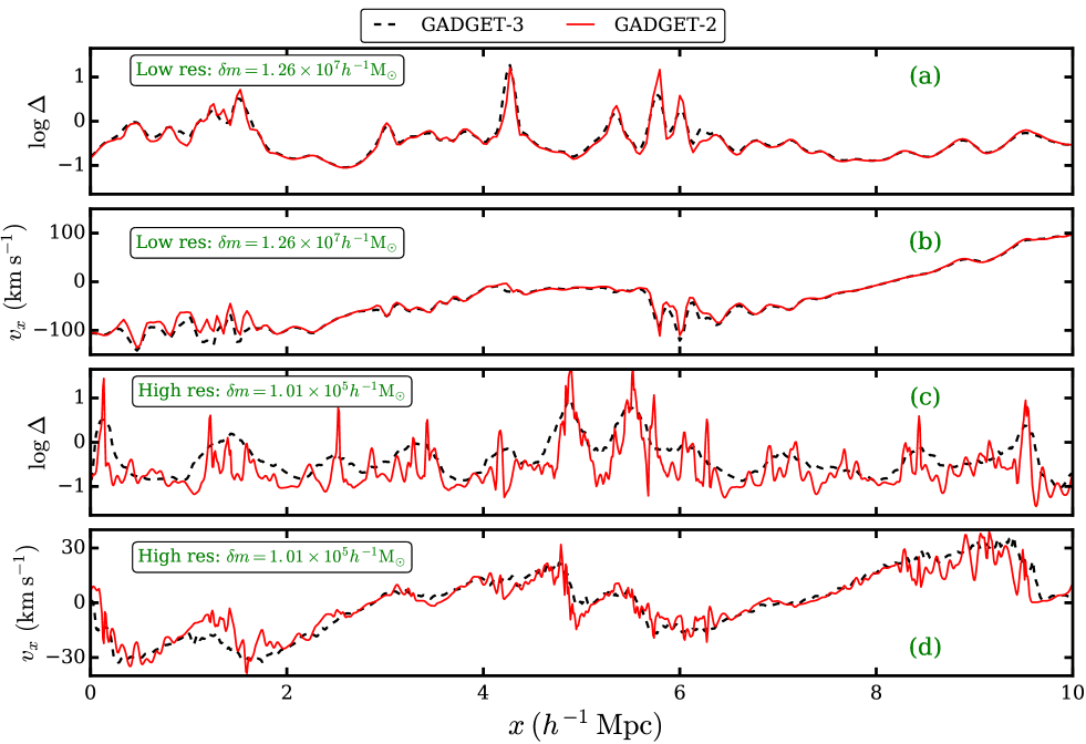
Figure 1: Panels (a) and (b) compare the line of sight density and velocity fields respectively from gadget-3 (black dashed curve) and gadget-2 (red solid curve) simulations for a low resolution simulation box at $z=2.5$ (box size $L=50h^{-1}$ cMpc, gas particle mass $\delta m=1.26\times 10^{7}\>h^{-1}\>{\rm M}_{\sun}$ and pixel size $\delta x=48.8h^{-1}$ ckpc). Panels (c) and (d) are same as panels (a) and (b) respectively except that these are obtained from high resolution simulation boxes at $z=2.5$ (box size $L=10h^{-1}$ cMpc, gas particle mass $\delta_{m}=1.01\times 10^{5}\>{\rm M}_{\sun}$ and pixel size $\delta x=9.77h^{-1}$ ckpc) used in this paper. gadget-2 models for low and high resolution boxes are performed with the temperature floor of $\sim 100$ K.

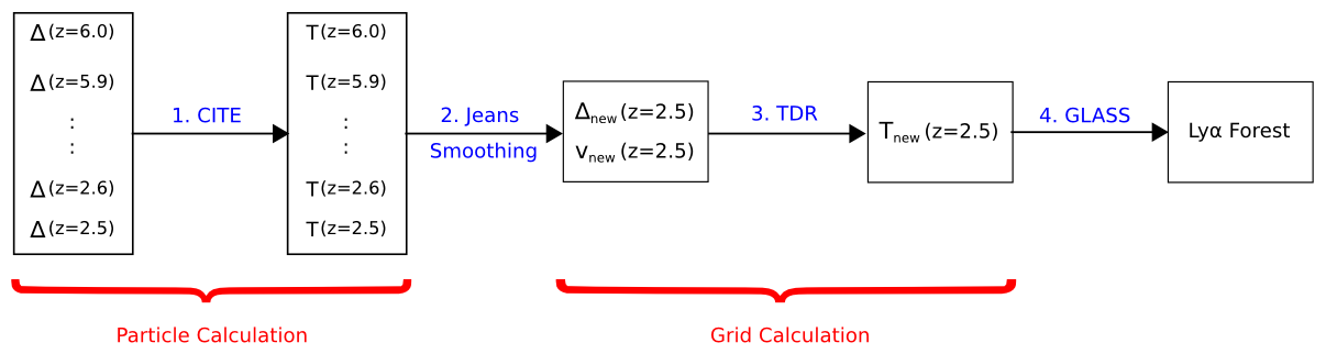
Figure 2: Schematic diagram showing main steps adopted in our post-processing method of obtaining  Ly$\alpha$ forest spectra from gadget-2 taking into account radiative cooling and heating effects externally. The basic steps involved in our method are: (1) We calculate the temperature of each particle at each redshift using cite and obtain the thermal history parameters $T_{0}$ and $\gamma$. (2) Given $T$ and $\Delta$ of particles, we apply pressure smoothing to get new $\Delta_{\rm new}$ and $v_{\rm new}$ on grids for a simulation box at a redshift of interest. (3) For this new $\Delta$ on grid points, we apply power-law TDR using thermal history parameters $T_{0}$ and $\gamma$ obtained in the previous step. (4) We calculate  Ly$\alpha$ optical depth from the simulation box using our routine glass.

We use the publicly available gadget-2 (Springel, 2005) to perform smoothed particle hydrodynamical simulations used in this study. The initial conditions are generated at $z=99$ using the publicly available 2lpt code (Scoccimarro et al., 2012). We use $1/30^{\rm th}$ of the mean inter-particle distance as the gravitational softening length. The gadget-2 simulation does not include radiative heating and cooling of the SPH particles internally. As a result, the unshocked gas particles (in the low density regions) are evolved at very low temperature (the default value is $100$ K in gadget-2) and pressure. However, the simulation allows one to set the minimum allowed gas temperature (referred as temperature floor) to higher values. In this work, we perform two simulations of gadget-2: (i) G2-LTF with low temperature floor of $T=100$ K and (ii) G2-HTF with high temperature floor of $T=10000$ K (corresponding to typical IGM temperatures due to photoheating). An unique identification number is assigned to each particle in gadget-2 and is used for tracing its density and temperature evolution.

We also perform a gadget-3 simulation (a modified version of the publicly available gadget-2 code, see Springel, 2005) with the same initial conditions as the gadget-2 simulations discussed above. Unlike gadget-2, the gadget-3 simulation includes radiative heating and cooling of SPH particles internally for any given metagalactic UV background (UVB). We use Haardt & Madau (2012, hereafter HM12) UVB assuming ionization equilibrium in gadget-3. To speed up the calculations, we run the simulations with QUICK_LYALPHA flag that converts particles with $\Delta>1000$ and $T<10^{5}$ K into stars (Viel et al., 2004a) and removes them from subsequent calculations. None of our simulations (i.e., gadget-2 or gadget-3) include AGN feedback, stellar feedback or outflows in the form of galactic wind. The details of our simulations are listed in Table 1.

Table 1: Details of our simulations described in §2

Model	gadget-3	G2-LTF	G2-HTF
N-body code	gadget-3	gadget-2	gadget-2
Initial redshift1	99	99	99
Box size ($h^{-1}$ c Mpc)	10	10	10
Number of particles	$2\times 512^{3}$	$2\times 512^{3}$	$2\times 512^{3}$
UVB2	HM12	HM12	HM12
Ionization evolution2	Equilibrium	Equilibrium	Equilibrium
$T$ and $\Delta$ evolution	Internal	Post-process (cite)	Post-process (cite)
SFR Criteria3	QUICK_LYALPHA	$-$	$-$
Output redshifts	$6.0,5.9,\cdots,2.0$	$6.0,5.9,\cdots,2.0$	$6.0,5.9,\cdots,2.0$
Temperature floor4	$-$	$100$ K	$10000$ K
Smoothing kernel type5	SPH	Modified	Modified
	$W(r,h)$	$W^{\prime}(r,h,L_{j})$	$W^{\prime}(r,h,0.66\times L_{J})$
Gas particle mass ($\delta m$)6	$1.01\times 10^{5}\>h^{-1}\>{\rm M}_{\sun}$	$1.01\times 10^{5}\>h^{-1}\>{\rm M}_{\sun}$	$1.01\times 10^{5}\>h^{-1}\>{\rm M}_{\sun}$
Pixel size ($\delta x$)7	$9.77h^{-1}$ ckpc	$9.77h^{-1}$ ckpc	$9.77h^{-1}$ ckpc

• All simulations (i.e. gadget-3, G2-LTF and G2-HTF) are performed using same initial condition.

• The default run of gadget-3 solves equilibrium ionization evolution equation using HM12 UVB.

• The QUICK_LYALPHA flag in gadget-3 converts gas particles with $\Delta>1000$ and $T<10^{5}$K in to stars.

• The minimum allowed temperature of the gas particle in simulation is set by the temperature floor.

• To account for pressure smoothing in G2-LTF and G2-HTF model, the smoothing kernel is modified by convolving SPH kernel with Gaussian kernel of pressure smoothing in the post-processing step. The pressure smoothing is self-consistently accounted for in the default run of gadget-3 model.

• The gas particle mass refers to the minimum mass of baryon particles in our model runs.

• The pixel size refers to the scale on which quantities (like $\Delta$, $v$ and $T$) are gridded when computing the spectra.

3 Method

The  Ly$\alpha$ optical depth is calculated by evaluating the overdensity ($\Delta$), temperature ($T$) and velocity ($v$) on grid points along a given sightline in the simulation box. Unlike gadget-3, the TDR obtained in gadget-2 is not realistic as the radiative heating and cooling terms are not incorporated. At moderate to low resolution, the overdensity and velocity fields from gadget-2 matches well with those from gadget-3 as shown in panel (a) and (b) of Fig. 1. This resolution (gas particle mass $\delta m=1.26\times 10^{7}\>h^{-1}\>{\rm M}_{\sun}$, pixel size $\delta x\sim 48.8h^{-1}$ ckpc) is appropriate for low-$z$ ($z<0.5$)  Ly$\alpha$ forest studies with instruments like the HST-COS (Gaikwad et al., 2017a, b). However gadget-2 does not capture the effect of finite gas pressure in the hydrodynamical evolution of the photoionized gas. This effect becomes important at smaller scales probed well in high resolution spectra (gas particle mass $\delta m=1.01\times 10^{5}\>h^{-1}\>{\rm M}_{\sun}$, pixel size $\delta x\sim 9.77h^{-1}$ ckpc) typically used in the  Ly$\alpha$ forest studies at high-$z$ ($z>1.6$). This is illustrated in the panel (c) and (d) of Fig. 1 where the density and velocity fields obtained in gadget-3 can be seen to be smooth as compared to those in gadget-2. Our method of evolving the gas temperature using gadget-2 + cite, as discussed in Gaikwad et al. (2017a), does not account for the effect of finite gas pressure on the evolution of density and velocity fields.

In this work, we present a method to account for the effect of gas pressure in gadget-2 + cite for high resolution  Ly$\alpha$ forest simulations. Fig. 2 shows the outline of our procedure whose main steps are as follows: (1) First we estimate the temperature of the gadget-2 particles accounting for the radiative heating and/or cooling (Gaikwad et al., 2017a). Depending on the requirements of the problem, the ionized fraction can be calculated either under ionization equilibrium or non-equilibrium conditions. (2) We then calculate the Jeans length for each particle assuming the particles to be in local hydrostatic equilibrium (Schaye, 2001). We smooth the density field by modifying the SPH kernel suitably to account for pressure smoothing. (3) We then use the TDR to calculate the temperature on the grids (Hui & Gnedin, 1997) for particles that do not go through any shock heating. (4) Finally we calculate the  Ly$\alpha$ optical depth using the density, velocity and temperature along the sightline (Choudhury et al., 2001). We discuss all these steps in more details below.

3.1 Temperature evolution in gadget-2 using cite:

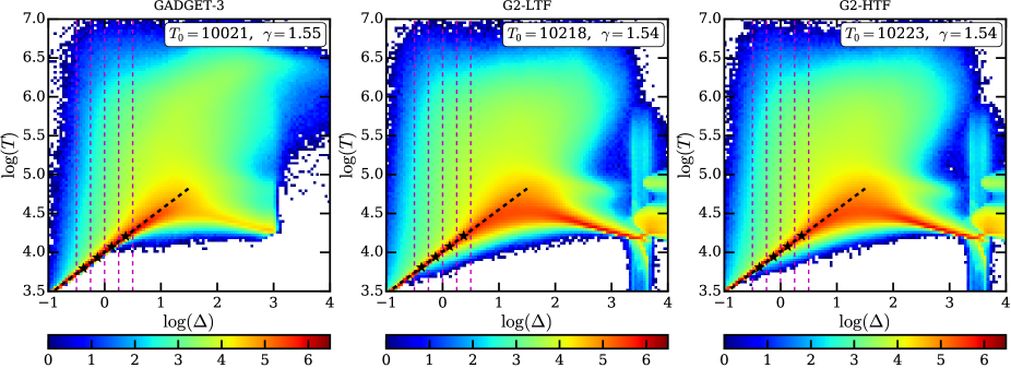
Figure 3: TDR of the SPH particles from gadget-3 (left panel), G2-LTF (middle panel) and G2-HTF (right panel) at $z=2.5$. The temperature in the G2-LTF and G2-HTF models are obtained in the post-processing step of gadget-2 using cite (see §3). The magenta dashed vertical lines show bins in $\log\Delta$. We calculate median $T$ (black stars) in each of these $\Delta$ bins and fit a power-law, $T=T_{0}\>\Delta^{\gamma-1}$, to obtain $T_{0}$ and $\gamma$. The resulting TDR is shown by black dashed line. In the case of gadget-3 we use quick_lyalpha flag under which gas particles with $T<10^{5}$ K and $\Delta>1000$ are converted into stars and got removed from subsequent calculations. No such star formation criteria is applied in G2-LTF and G2-HTF models (see Appendix A for more details). The colour scheme represents density of points in logarithmic unit.

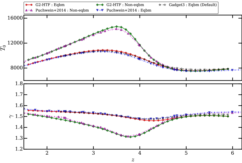
Figure 4: Comparison of redshift evolution of the thermal history parameters ($T_{0}$ and $\gamma$) from our G2-HTF with gadget-3 (gray stars) simulations and that of Puchwein et al. (2015, magenta up-triangles for non-equilibrium and blue down-triangles for equilibrium ionization evolution). cite is started at $z=6.0$ with initial conditions $T_{0}=7920$ K and $\gamma=1.52$ same as those obtained in gadget-3 at that redshift (see §3 for details). For G2-HTF simulations we run cite using equilibrium (red filled circles) and non-equilibrium (green diamonds) ionization condition influenced by the same UVB. Note that the default version of gadget-3 solves equilibrium ionization evolution equation.

We evolve the temperature of the particles in gadget-2 using cite (as discussed in details in Gaikwad et al., 2017a). For completeness, here we briefly discuss the steps involved. We solve the temperature evolution equation for each particle in the post-processing step of gadget-2 using

$$\frac{dT}{dt}=-2HT+\frac{2T}{3\Delta}\>\frac{d\Delta}{dt}+\frac{dT_{\rm shock}}{dt}+\frac{dT_{\rm IE}}{dt}+\frac{dT_{\rm other}}{dt}\;\;.$$ (1)

The five terms on the right hand side of above equation represents, respectively, rate of cooling due to Hubble expansion, adiabatic heating or cooling arising from change in density of particles, change in temperature due to shock heating, change in temperature due to change in internal energy per particle and change in temperature due to other heating/cooling processes (such as photo-heating, cosmic ray heating, radiative cooling). We use cite to calculate the last two terms on right hand side of Eq. 1 as they are not self-consistently computed in gadget-2. The actual implementation is as follows.

1. At the initial redshift (taken to be $z_{1}=6.0$ in this work), we assume a given power-law TDR. In this paper, we choose $T_{0}=7920$ K and $\gamma=1.52$ in order to match those obtained in gadget-3 at the same redshift for HM12 UVB. We then compute the actual temperature of a gas particle using following prescription: If a particle is shock heated in recent times (i.e., within a time scale corresponding to $\delta z=0.1$), then the temperature of the particle will not be updated by cite. Otherwise we assume the particle temperature to be following the above mentioned power-law TDR. At the initial redshift, we solve equilibrium ionization evolution equation assuming HM12 UVB to calculate various ion fractions of H and He.

2. Given the ion fractions and the temperatures, it is straightforward to calculate last two terms on the right hand side of Eq. 1 for subsequent time steps. For this, we use the photo-heating rates of HM12 UVB model.

3. To obtain the temperature of the particles in the next time step ($z_{2}=z_{1}-\Delta z$), we first check if the particle is shock heated in recent times (i.e., within a time scale corresponding to $\delta z=0.1$). If the particle is not shock heated, then we neglect the third term on the right hand side of Eq. 1. Otherwise we solve the same Eq. 1 accounting all the five terms.

4. For redshift $z_{2}$, we solve equilibrium (or non-equilibrium, if desired) ionization evolution equations to calculate various ion fractions.

5. We repeat the steps (ii)-(iv) to obtain the temperature of the particle at subsequent redshifts.

Fig. 3 shows comparison of TDR of SPH particles obtained from gadget-3 (left panel), G2-LTF (middle panel) and G2-HTF (right panel) simulations at $z=2.5$. Qualitatively, the TDR from G2-LTF and G2-HTF (after processing through cite) is remarkably similar to that from gadget-3. The differences at $\Delta>1000$ and $T<10^{5}$ K can be attributed to the QUICK_LYALPHA flag employed in gadget-3 (see Appendix A for more details). For each model, we calculate median temperature (black star points) in $\log\Delta$ bins with centres at $-0.375,-0.125,0.125,0.375$ and bin width $0.125$ (indicated by magenta dashed vertical lines). We then fit power law relation $T=T_{0}\>\Delta^{\gamma-1}$ to obtain the best fit $T_{0}$ and $\gamma$ (Hui & Gnedin, 1997; McDonald et al., 2005). The fitted TDR is shown by black dashed line in each panel. The values of $T_{0}$ and $\gamma$ are also indicated in each panel. It is clear that they are similar within $2.5$ percent.

Fig. 4 shows the redshift evolution of best fit $T_{0}$ (top panel) and $\gamma$ (bottom panel) for G2-HTF, gadget-3 and Puchwein et al. (2015) models for equilibrium and non-equilibrium ionization evolution cases. The evolution of $T_{0}$ and $\gamma$ obtained from cite for the equilibrium ionization case is remarkably similar to those obtained from the gadget-3 run and Puchwein et al. (2015). As mentioned earlier, we can also solve for non-equilibrium ionization evolution equation using cite. The $T_{0}$ and $\gamma$ evolution for non-equilibrium case from Puchwein et al. (2015, magenta dashed curve) is also consistent with those from G2-HTF with the maximum difference being less than 2.5 per cent (at $z\sim 3.5$). Since the default version of gadget-3 solves the ionization evolution equation under equilibrium conditions, hereafter we restrict our discussions to the models with equilibrium ionization as we will use gadget-3 as our reference. While cite reproduces the $T_{0}$ and $\gamma$ evolution well, the issues related to small scale density and velocity field (demonstrated in Fig. 1) still need to be addressed.

3.2 Jeans length of SPH particle in gadget-2:

In this section, we explore the possibility of using local pressure smoothing in the gadget-2 simulations to reduce the shortcomings highlighted in panels (c) and (d) of Fig. 1. We choose to smooth the density field in G2-LTF or G2-HTF on the scales of Jeans length of the particles to account for the pressure smoothing. Assuming the  Ly$\alpha$ absorbers to be in local hydrostatic equilibrium, Schaye (2001) has shown that the Jeans length can be obtained by equating dynamical time with sound crossing time and is given by,

$${}\frac{L}{1\>{\rm kpc}}\sim 0.52\>\bigg{[}\frac{T}{10^{4}\>{\rm K}}\>\frac{1-Y}{0.76}\>\frac{f_{g}}{0.16}\>\frac{1\>{\rm cm}^{-3}}{n_{H}}\>\frac{0.59}{\mu}\bigg{]}^{1/2}$$ (2)

where, $T$ is temperature, $n_{H}$ is number density of H, $Y$ is He fraction by mass, $\mu=4/(8-5Y)$ is the mean molecular weight and $f_{g}$ is fraction of total mass in gas phase. For the scales of interest here $f_{g}$ is close to its universal value $\Omega_{\rm b}/\Omega_{\rm m}\sim 0.16$. It should be emphasized that the Jeans length depends on the density and temperature and hence is different for different particles. For the same reason, it is different for the same particle at different epochs. The above equation is not valid for  Ly$\alpha$ absorbers with characteristic densities smaller than the cosmic mean ($\Delta\sim 1$, Schaye, 2001). Hence we ignore the pressure smoothing for such particles and retain only the SPH smoothing. We now explain how the effect of pressure smoothing is incorporated in G2-LTF or G2-HTF by modifying the SPH kernel.

Smoothing kernel :

The estimate of a quantity $f$ at any grid point $i$ in the SPH formulation (Monaghan, 1992; Springel, 2005) is given by,

$${}f_{i}=\sum\limits_{j}\;f_{j}\;\frac{m_{j}}{\rho_{j}}\;S_{ij}$$ (3)

where the summation is performed over all particles. The quantities $m_{j}$, $\rho_{j}$, $f_{j}$ are the mass, density and value of the quantity $f$ of $j^{th}$ particle, respectively. The quantity $f$ could be overdensity ($\Delta$), temperature ($T$) or any component of the velocity ($v$). The smoothing kernel, $S_{ij}$, has units of inverse of volume and in general depends on the distance ($r_{ij}$) between $i^{th}$ grid point and $j^{th}$ particle. It is necessary for $S_{ij}$ to satisfy the following normalization condition in order to conserve the quantity $f$ (in particular mass) in SPH formulation (Monaghan, 1992),

$${}\int\limits_{\mathcal{V}}\;S_{ij}\;d\bm{r}=1$$ (4)

where the integration is over volume $\mathcal{V}$.

We use the following smoothing kernels for various simulations,

$${}S_{ij}\equiv\begin{cases}\;\;W(r_{ij},h_{j}),&{\rm For\;\textsc{gadget-3}}\\ \;\;W^{\prime}(r_{ij},h_{j},1\times L_{j}),&{\rm For\;\textsc{{}{G2-LTF}}}\\ \;\;W^{\prime}(r_{ij},h_{j},0.66\times L_{j}),&{\rm For\;\textsc{{}{G2-HTF}}}\\ \end{cases}$$ (5)

where $h_{j}$ and $L_{j}$ are smoothing length and Jeans length (given by Eq. 2) of the $j^{th}$ particle respectively.

The smoothing kernel used for gadget-3 is same as SPH kernel given in Springel (2005) and has following form,

$$W(r,h)=W_{0}\begin{cases}\;\;1-6\bigg{(}\frac{r}{h}\bigg{)}^{2}+6\bigg{(}\frac{r}{h}\bigg{)}^{3},&0\leq\frac{r}{h}\leq\frac{1}{2}\\ \;\;2\bigg{(}1-\frac{r}{h}\bigg{)}^{3},&\frac{1}{2}\leq\frac{r}{h}\leq 1\\ \;\;0,&\frac{r}{h}>1\end{cases}$$ (6)

where $W_{0}=8/(\pi h^{3})$ is normalization constant of SPH kernel.

The pressure smoothing can be well approximated by a Gaussian (Gnedin & Hui, 1998; Kulkarni et al., 2015). Hence we modify the smoothing kernel by convolving SPH kernel with Gaussian kernel of pressure smoothing

$$W^{\prime}(r,h,\sigma) =\int\>{\rm d}^{3}\bm{x_{1}}\>W(r_{1},h)\;G(|\bm{r}-\bm{x_{1}}|,\sigma)\;$$ (7)

where the Gaussian kernel is assumed to be isotropic and is given by

$$G(|\bm{r}-\bm{x_{1}}|,\sigma) =\frac{1}{(2\pi\sigma^{2})^{3/2}}\;\;{\rm exp}\bigg{[}{-\frac{|\bm{r}-\bm{x_{1}}|^{2}}{2\sigma^{2}}}\bigg{]}$$ (8)

$$=\frac{1}{(2\pi\sigma^{2})^{3/2}}\;\;{\rm exp}\bigg{[}{-\frac{(r^{2}+r_{1}^{2}-2\>r\>r_{1}\>\mu)}{2\>\sigma^{2}}}\bigg{]}$$

with $\mu$ being the cosine of the angle between $\bm{r}$ and $\bm{x_{1}}$ and $\sigma$ the width of the Gaussian which in turn depends on the Jeans length. At this point let us highlight some of the key properties of $W^{\prime}(r,h,\sigma)$ which are relevant for our calculations:

• Both $W(r,h)$ in Eq. 6 and $W^{\prime}(r,h,\sigma)$ in Eq. 7 satisfy the normalization condition given in Eq. 4.

• The kernel in Eq. 7 does not have a closed form analytic solution, hence we need to calculate it numerically (See Appendix B for more details).

• Unlike $W(r,h)$, $W^{\prime}(r,h,\sigma)$ does not have a compact support as the Gaussian is non-zero at large distances. Hence we put a cut-off such that if distance between particle and grid is more than $h+3\sigma$, the contribution of $W^{\prime}(r,h,\sigma)$ is zero. Mathematically,

  $$W^{\prime}(r,h,\sigma)=\begin{cases}\;\;W^{\prime}(r,h,\sigma)&0\leq r\leq(h+3\sigma)\\ \;\;0,&r>(h+3\sigma)\;\;\;\;\;.\end{cases}$$ (9)

  We find that this cut-off does not have any significant effect on the density, velocity or temperature estimates as long as it is taken to be $\geq h+3\sigma$.

• The amount of pressure smoothing in Eq. 7 is decided by the width $\sigma$ of the Gaussian. The SPH particles in G2-HTF are evolved at relatively high temperature ($T\sim 10^{4}$ K) and pressure as compared to G2-LTF ($T\sim 100$ K). It can be shown that the additional pressure smoothing length required in G2-HTF model is factor $\sim 0.66$ times the smoothing length for the model G2-LTF (see Appendix C for details).

• This way of modifying smoothing kernel and estimating quantities along sightlines allow us to account for two important effects: (i) the variation in pressure smoothing for different particles at any epoch and (ii) the evolution of pressure smoothing scale for any particle at different epochs. Note that the pressure smoothing experienced by a particle in the gadget-3 simulation depends on the whole thermal history and not only on the present temperature as we do in our case (Lukić et al., 2015; Kulkarni et al., 2015). However, as we will discuss later, running the gadget-2 with high temperature floor captures (on an average) the pressure broadening arising from thermal history effects reasonably well.

3.3 Estimation of the temperature field on a grid:

After calculating the overdensity ($\Delta$) and velocity field ($v$) on grids along a given sightline using Eqs 3-8, we can also estimate the temperature ($T$) along the same sightline using the same equations. However, the resultant TDR is not a power-law any more. This is because the temperature of the particle from cite in the first step is calculated using gadget-2 density field that does not incorporate the pressure smoothing. Hence we need to recalculate the temperature corresponding to the new density field with the pressure smoothing incorporated. In principle, we can again use cite on the new smoothed density field and calculate the temperature. However, we find that this is computationally expensive because we need to calculate the smoothed density field on the grid along the sightline for all redshifts i.e. $z=6$ to $2$ with a $\Delta z=0.1$. Hence we adopt a simplified approach of applying power-law TDR (Hui & Gnedin, 1997; Choudhury et al., 2001)

$$T=\begin{cases}\;\;T_{0}\;\Delta^{\gamma-1},&\Delta\leq 10\\ \;\;T_{0}\;10^{\gamma-1},&\Delta>10\\ \;\;T_{\rm shock},&T_{\rm shock}>T\end{cases}$$ (10)

where $T_{0}$ and $\gamma$ are obtained from fitting the TDR for particles in our simulation box at the redshift of our interest as explained in Step (1) (also see Fig. 4). The last relation implies that if a particle is shock heated (or has temperature higher than that predicted by the TDR) then its temperature is not updated. We have confirmed that this approach produces consistent results with those obtained by running cite on the new density field.

3.4  Ly$\alpha$ transmitted flux:

We have developed a module for “Generating Ly-Alpha forest Spectra in Simulations” (glass) to calculate the  Ly$\alpha$ transmitted flux that has signal-to-noise ratio (SNR) and spectral resolution similar to the typical observational data used in the  Ly$\alpha$ forest studies. The basic steps involved in glass (Choudhury et al., 2001; Padmanabhan et al., 2015; Gaikwad et al., 2017a) are as follows:

1. We determine the Hi number density ($n_{\rm HI}$) at any grid point from the baryonic density field ($\Delta$) assuming the gas to be optically thin and in photoionizing equilibrium with the UVB. The Hi photoionization rate ($\Gamma_{\rm HI}$) is a free parameter. Throughout this paper we consider models with a fixed value $\Gamma_{\rm HI}$ $=10^{-12}\;{\rm s}^{-1}$ (Becker & Bolton, 2013) for simplicity.

2. We calculate the  Ly$\alpha$ optical depth ($\tau$) along a line of sight from $n_{\rm HI}$ field by accounting for peculiar velocity, thermal and natural broadening effects.

3. The  Ly$\alpha$ transmitted flux is given by $F={\rm e}^{-\tau}$.

4. When comparing with observations, the  Ly$\alpha$ flux field is linearly interpolated to match the wavelength sampling of observations.

5. The  Ly$\alpha$ flux field is then convolved with line spread function (LSF) of the spectrograph used in the observation. In this work we assume that the LSF is a Gaussian with a full width at half maximum, FWHM $\sim 7$  km s^-1, typical of UVES or HIRES spectra.

6. Finally we add Gaussian random noise corresponding to a typical SNR=25 similar to what has been frequently achieved in echelle spectrographic observations with VLT and KECK that are used for  Ly$\alpha$ forest studies.

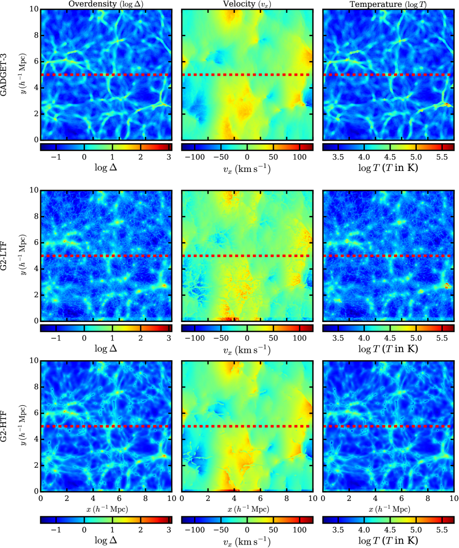
Figure 5: Slices from a simulation box having a width $\sim 10$ ckpc at $z=2.5$ for gadget-3 (top), G2-LTF (middle) and G2-HTF (bottom). Left, middle and right panels in each row show overdensity ($\log\Delta$), velocity component ($v_{x}$) along $x$ axis and temperature ($\log T$) field respectively. The colour scheme represents density of points in logarithmic unit. We shoot a sightline parallel to $x$ axis through simulation box in each model as shown by horizontal dashed line in each panel. The extracted $\log\Delta$, $v_{x}$ and $\log T$ along these sightlines are plotted in Fig. 6 .

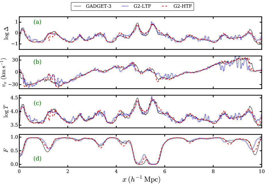
Figure 6: Comparison of line of sight overdensity (panel (a), $\log\Delta$), velocity (panel (b), $v_{x}$ in  km s^-1), temperature (panel (c), $\log T$) and  Ly$\alpha$ transmitted flux (panel (d), $F$) for gadget-3 (black solid line), G2-LTF (blue dotted line) and G2-HTF (red dashed line) from a simulation box at $z=2.5$ shown in Fig. 5. The  Ly$\alpha$ transmitted flux is not convolved with any LSF and no noise is added to the flux.

A comparison of slices (having a width of $10$ ckpc) of the overdensity ($\log\Delta$), line of sight velocity (along $x$ axis, $v_{x}$) and temperature ($\log T$) fields on grids from a simulation boxes at $z=2.5$ are shown in Fig. 5. The top, middle and bottom rows show slices from gadget-3, G2-LTF and G2-HTF simulations respectively. The $\log\Delta$, $v_{x}$ and $\log T$ fields are sharper in the G2-LTF model (in particular in low density regions) as compared to those of gadget-3 model. On the other hand the $\log\Delta$, $v_{x}$ and $\log T$ fields from G2-HTF model resembles close to those from gadget-3. We shoot a sightline through each of these slices as shown by horizontal dashed line and extract the $\log\Delta$, $v_{x}$ and $\log T$ fields as shown in panel (a), (b) and (c) of Fig. 6 respectively. The line of sight $\log\Delta$, $v_{x}$ and $\log T$ fields from G2-LTF and G2-HTF are very similar to those from gadget-3. However, in general the variations in these fields for G2-LTF model are slightly more compared to those of gadget-3 and G2-HTF models. The panel (d) of Fig. 6 shows the  Ly$\alpha$ transmitted flux calculated along sightlines shown in Fig. 5 for gadget-3, G2-LTF and G2-HTF models. Visually the  Ly$\alpha$ transmitted fluxes from different models are similar, despite subtle differences seen in $\log\Delta$, $v_{x}$, $\log T$ fields between these models. The  Ly$\alpha$ transmitted flux shown in this example is not convolved with LSF and is free of noise.

To perform a quantitative comparison of the  Ly$\alpha$ forest spectra extracted from different models, we identify eight statistics that are frequently used in the literature. We shoot random sightlines through the simulation and splice together the lines of sight in such a way that it covers a redshift path $z\pm 0.05$, where $z=2.5,3.0,3.5,4.0$ are redshifts of the simulation box. Each  Ly$\alpha$ forest spectrum has a path length of $\sim 50$ cMpc. Following Rollinde et al. (2013); Gaikwad et al. (2017a, b), we generate a mock sample of $N_{\rm spec}=20$  Ly$\alpha$ forest spectra for the gadget-3, G2-LTF and G2-HTF models. Each mock sample covers path length of $\sim 1000h^{-1}$ cMpc (corresponding dimensionless absorption path length is $X\sim 5.35$ at $z=3$). This path length is similar to the path length covered in the  Ly$\alpha$ forest studies by Becker et al. (2011, see their Table 3). We repeat the procedure by choosing different random sightlines and generate $N=100$ such mock samples. The collection of $N$ mock samples constitute a “mock suite” that consists of $N\times N_{\rm spec}=2000$ simulated spectra. Thus total path length covered in mock suite is $\sim 10^{5}$ cMpc. We estimate the covariance matrix for different statistics using the simulated spectra.

4 Results

We now compare different properties of the  Ly$\alpha$ forest generated from G2-LTF, G2-HTF and gadget-3 simulations using eight statistics, namely, (i) the line of sight baryonic density field ($\delta=\Delta-1$) power spectrum (DPS), (ii) the flux probability distribution function (FPDF), (iii) the flux power spectrum (FPS), (iv) the wavelet statistics, (v) the curvature statistics, (vi) the column density distribution function (CDDF), (vii) the line width ($b$) distribution function and (viii) the $b$ vs  $\log{\rm N_{HI}}$ scatter plot. The statistics (i)-(v) are obtained assuming  Ly$\alpha$ transmitted flux to be a continuous field whereas, the statistics (vi)-(viii) are based on parameters derived using Voigt profile decomposition of  Ly$\alpha$ forest. For this purpose we use our automatic Voigt profile fitting code viper described in full detail in Gaikwad et al. (2017b).

4.1 Line of sight density power spectrum (DPS)

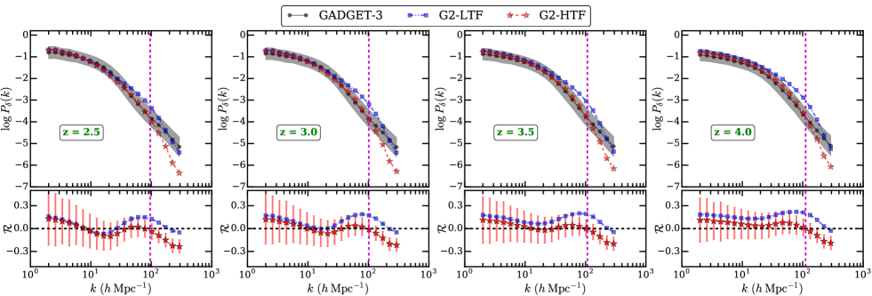
Figure 7: Top left panel shows the comparison of the line of sight density field power spectrum obtained from gadget-3 (black circle), G2-LTF (blue squares) and G2-HTF (red stars) models at $z=2.5$. The gray shaded region represents the $1\sigma$ uncertainty (diagonal elements of covariance matrix given in Eq. 13) on the DPS from gadget-3. The Fourier modes with $k>k_{\rm cutoff}$ ($k_{\rm cutoff}$ varies with redshift e.g., $k_{\rm cutoff}(z=3)\sim 101h$ Mpc^-1, magenta dashed vertical line) are not be probed by current observations due to limited velocity resolution ($\sim 7$  km s^-1) of the spectra. The residuals ($\mathcal{R}$, see Eq. 14) between the G2-LTF, G2-HTF models with respect to the gadget-3 model at $z=2.5$ are shown in bottom left panel. The error-bars shown in this panel represent the $1\sigma$ uncertainties generated from a path length of $1000h^{-1}$ cMpc (corresponding dimensionless absorption path length is $X\sim 5.35$ at $z=3$) which correspond to the gray shaded region in the top left panel. The DPS from G2-LTF and G2-HTF models are within 12 and 18 percent of gadget-3 model at scales $k<k_{\rm cutoff}$. The other panels show similar comparison at $4$ different redshifts that are identified in each panel.

The density field power spectrum is not a directly measurable quantity but it influences all the observable quantities of  Ly$\alpha$ forest. We calculate the power spectrum of the 1D density fluctuations along the line of sights using sightlines of comoving length equal to the simulation box size $10\>h^{-1}$ cMpc. This is done by computing the Fourier transform $\delta(k)$ of the density field $\delta(x)$, the corresponding power is simply given by $P_{\delta}(k)\propto|\delta(k)|^{2}$. We normalize the DPS (Zhan et al., 2005) as,

$$\sigma^{2}_{F_{\delta}}=\int\limits_{-\infty}^{\infty}\frac{dk}{2\pi}\;P_{\delta}(k)$$ (11)

where $\sigma^{2}_{F_{\delta}}$ is variance of the 1D density field. We bin the DPS in $20$ equispaced logarithmic bins in the range $\log k=0.301$ to $2.466$ with bin width of $\Delta\log k=0.114$ (Kim et al., 2004).

Following Rollinde et al. (2013) and Gaikwad et al. (2017a), we take the average of all DPS along different sightlines in a mock sample (consisting of $20$ lines of sight). We then calculate the mean DPS and the associated errors from the mock suite (which consists of $N=100$ mock sample). Let $P_{\delta,n}(k_{i})$ denotes the value of DPS in $i^{th}$ bin of $n^{th}$ mock sample, then the average DPS in $i^{th}$ bin is given by,

$$\overline{P}_{\delta}(k_{i}) =\frac{1}{N}\;\sum\limits_{n=1}^{N}P_{\delta,n}(k_{i})\;\;.$$ (12)

The covariance matrix element $C(i,j)$ between the $i^{th}$ and $j^{th}$ bins is given by,

$$C(i,j) =\frac{1}{N-1}\;\sum\limits_{n=1}^{N}[\overline{P}_{\delta}(k_{i})-P_{\delta,n}(k_{i})][\overline{P}_{\delta}(k_{j})-P_{\delta,n}(k_{j})]$$ (13)

where, $i$ and $j$ can take values from 1 to the number of bins. The above analysis assumes a mock sample path length of 1000$h^{-1}$ cMpc (i.e., the mock sample consisting of $20$ spectra, corresponding dimensionless absorption path length is $X\sim 5.35$ at $z=3$). We have done the similar analysis for the $5000h^{-1}$ cMpc mock sample path length (i.e., the mock sample consisting of $100$ spectra, corresponding to $X\sim 26.75$ at $z=3$). In this case we find that the covariance matrix elements are similar to those from mock samples with $1000h^{-1}$ cMpc path length for all the statistics (see the discussion in Appendix D). Hereafter unless mention the results are presented for mock sample path length of $1000h^{-1}$ cMpc.

The top left panel of Fig. 7 shows the DPS for the gadget-3 (black circles), G2-LTF (blue squares) and G2-HTF (red stars) models at $z=2.5$. The grey shaded region is the $1\sigma$ uncertainty coming from sample variance (i.e., variation in DPS along different sightlines) in the gadget-3 DPS. The bottom left panel shows the residual fraction (hereafter residual for simplicity) between G2-LTF (blue squares) and G2-HTF (red stars with errorbars) model with respect to gadget-3 model. The residual between G2-HTF (or G2-LTF) and gadget-3 model is defined as follows,

$$\mathcal{R}_{\rm{}{G2-HTF}}=1-\frac{P_{\delta,{\rm{}{G2-HTF}}}}{P_{\delta,{\rm GADGET-3}}}\;\;\;\;.$$ (14)

The errors on G2-HTF residuals in bottom left panel of Fig. 7 correspond to grey shaded region in top left panel (sample variance). Other panels in Fig. 7 are similar to left most panels but for different redshifts. The redshifts are mentioned in each panel.

Although we show the DPS in the range $1\leq k\leq 300h\>{\rm Mpc}^{-1}$, all these scales are not accessible in the current set of best possible spectroscopic observations. The first scale is introduced by the typical temperature of the IGM at cosmic mean density $\sim 10^{4}$ K which corresponds to a velocity smoothing of $\sim 12$  km s^-1. The second scale is spectral resolution of $\sim 7$  km s^-1achieved by the current echelle spectrographs like HIRES or UVES. Thus scales below $\sim 7$  km s^-1or the Fourier modes above the cut-off scale $k_{\rm cutoff}(z=3)=101h\>{\rm Mpc}^{-1}$ ($k_{\rm cutoff}$ varies with redshift and is shown by magenta dashed vertical line) cannot be probed by  Ly$\alpha$ forest observations. Note that the velocity sampling of our simulated mock spectra is $\sim 1.11$  km s^-1.

We find that at all redshifts the DPS for G2-HTF and G2-LTF are within 12 and 18 percent (and well within $1\sigma$ uncertainty due to sample variance) respectively with that from gadget-3 at $k\leq k_{\rm cutoff}$. The G2-LTF model has higher power on the scales in the range 35-135 ckpc ($k\sim 180-47\>h$  Mpc^-1). Note that although the instantaneous TDR is similar in G2-HTF and G2-LTF model (see Fig. 3), the thermal history of the particles is different because the particles in G2-LTF model that do not go through shocks are effectively evolved at temperature smaller by factor of 100 as compared to those in G2-HTF. The pressure smoothing scale, in addition to instantaneous TDR, also depends on thermal history of the particles (Kulkarni et al., 2015). Thus the density field in G2-LTF model is less smooth (and hence has more power) as compared to that from G2-HTF model at small scales. This difference is more prominent at high redshifts. This highlights the need for an appropriate smoothing of the density field on scales larger than pressure smoothing scale for G2-LTF at higher redshifts. However, when we evolve our simulations with a high temperature floor (i.e., $T\sim 10^{4}$ K), Jeans length based on a instantaneous $T$ and $\Delta$ is adequate to capture the pressure smoothing effects over the scales probed by the  Ly$\alpha$ forest observations.

We notice at $k>k_{\rm cutoff}$, the power in G2-HTF model is smaller as compared to gadget-3 model. This is due to the fact that the minimum temperature before applying cite (irrespective of the density) in G2-HTF model is $\sim~{}10^{4}$ K. However in gadget-3 model, the particles with $\Delta<1$ are at temperature smaller than $10^{4}$ K (see Fig. 3). Thus higher temperature for $\Delta<1$ particles in G2-HTF model leads to an additional pressure smoothing, thus the power on scales $k>k_{\rm cutoff}$ is smaller than that from gadget-3. However it is important to note that (for reasons mentioned above) the mismatch between G2-HTF and gadget-3 model at $k>k_{\rm cutoff}$ does not have a significant effect on the  Ly$\alpha$ flux statistics presented later.

4.2 Flux probability distribution function (FPDF)

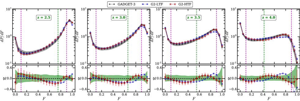
Figure 8: Top left panel and bottom left panels are similar to the corresponding panels in Fig. 7 but for the FPDF statistics. Unlike Fig. 7, the uncertainty in top (gray shaded region) and bottom (red stars with errorbars) left panel has contribution from the sample variance and finite noise added to the spectra. The green shaded region in the bottom panels represents sample variance for gadget-3 model calculated using noise free spectra (i.e., SNR$=\infty$). The FPDF is compared in the range $0.1\leq F\leq 0.9$ (shown by magenta dashed vertical lines) since the flux near continuum and saturated region is usually affected by observational systematics (see section 4.2 for details). The green dashed dot vertical line shows the mean flux for gadget-3 model. We present the results for $4$ redshifts whose values are mentioned in the corresponding panel. All the results are presented for SNR = 25, $\Gamma_{\rm 12}$ $=1$ and for mock sample path length of $1000h^{-1}$ cMpc (corresponding to $X\sim 5.35$ at $z=3$).

The FPDF is one of the flux statistics that is relatively straightforward to calculate from observations as well as simulations (Jenkins & Ostriker, 1991; McDonald et al., 2000; Kim et al., 2007; Desjacques et al., 2007; Rollinde et al., 2013; Gaikwad et al., 2017a). Note that we have added the noise to flux corresponding to the SNR of 25. Unless mentioned, hereafter all the results are presented for SNR=25 . We calculate the FPDF in $21$ equally spaced bins with bin centres in the range $F=0.05$ to $1.0$ and bin width $\Delta F=0.05$ (consistent with Kim et al., 2007). The pixels with $F<0$ ($F>1$) are included in the first (last) bin. Let $P_{n}(F_{i})$ denote the value of FPDF in $i^{th}$ bin of $n^{th}$ mock sample then average FPDF in $i^{th}$ bin (denoted as $\overline{P}(F_{i})$) is given by Eq. 12 where we replace $P_{\delta,n}(k_{i})$ with $P_{n}(F_{i})$. Similarly the covariance matrix element $C(i,j)$ between the $i^{th}$ and $j^{th}$ bins is obtained from Eq. 13 by replacing $P_{\delta,n}(k_{i})$, $\overline{P}_{\rm\delta}(k_{i})$ with $P_{n}(F_{i})$, $\overline{P}(F_{i})$ respectively.

Fig. 8 shows the comparison of FPDF obtained from gadget-3, G2-HTF and G2-LTF models. Various symbols and line styles are same as those used in Fig. 7. Note that for all the three models we use $\Gamma_{12}=1$, SNR=$25$ and a path length of $1000h^{-1}$ cMpc ($X\sim 5.35$ at $z=3$) for the mock sample. We calculated the mean FPDF, the covariance matrix and residuals ($\mathcal{R}$) using Eq. 12, 13 and 14 respectively with $P_{\rm\delta}$ replaced by $P_{\rm F}$. The $1\sigma$ uncertainty in top (gray shaded region) and bottom left panels (red stars with errorbars) are contributed by the uncertainty in FPDF along different sightlines (sample variance) and finite SNR of the spectra. In order to separate out the statistical error arising purely from the assumed SNR and that from the sample variance, we calculate the FPDF for noise free spectra (i.e. SNR$=\infty$ but same $\Gamma_{12}$ and mock sample path length) for gadget-3 model. The green shaded region in bottom panels of Fig. 8 represents sample variance from gadget-3 model. The size of this sample variance is comparable to the errors on FPDF from gadget-3 model (red stars with errorbars) suggesting that the errors are dominated by sample variance. The mean flux in gadget-3 model (shown by green dashed dot vertical line) differs by less than 0.78 percent with that from G2-HTF and G2-LTF models at all $z$.

The flux near the normalized continuum (in bins with $F>0.9$) is usually affected by two observational systematics, (i) the continuum fitting of the spectra and (ii) the noise property of the spectra. On the other hand, flux near saturated region ($F<0.1$) depends on accurate background sky subtraction. Thus while comparing observed FPDF and the simulated FPDF, one usually compares them in the range $0.1\leq F\leq 0.9$ (Gaikwad et al., 2017a). In Fig. 8, we compare the FPDF from three models within the range $0.1\leq F\leq 0.9$ shown by magenta dashed vertical lines.

It is clear from the bottom panels of Fig. 8 that the difference between FPDF in the range $0.1\leq F\leq 0.9$ for G2-HTF and G2-LTF (with respect to gadget-3 model) is less than $15$ and $18$ percent respectively at all redshifts. Note that sample variance is typically of the order of 13 percent in the range $0.1\leq F\leq 0.9$.

4.3 Flux power spectrum (FPS)

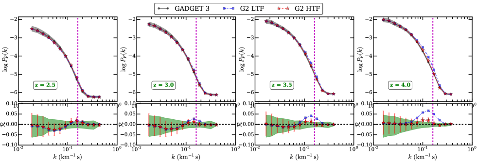
Figure 9: Comparison of FPS obtained from gadget-3, G2-LTF and G2-HTF models. The symbols and line styles are same as in Fig. 8. The FPS from G2-LTF and G2-HTF model is consistent within 5 percent with that from gadget-3 model (see section 4.3 for details). The magenta dashed vertical line shows the wavelet scale used in section 4.4.

Like the DPS, the FPS is a two point correlation function between pixels of the  Ly$\alpha$ transmitted flux (Croft et al., 1998; McDonald et al., 2000; McDonald, 2003; Kim et al., 2004; Zhan et al., 2005; Arinyo-i-Prats et al., 2015). The FPS is known to be sensitive to the astrophysical parameters such as $\Gamma_{\rm HI}$, $T_{0}$ and $\gamma$ (Zaldarriaga et al., 2001; Zaldarriaga, 2002; Viel et al., 2004a) in addition to the cosmological parameters. The procedure for calculating the FPS is identical to that of the DPS. If we denote the value of FPS in $i^{th}$ bin of $n^{th}$ mock sample as $P_{F,n}(k_{i})$ then the average FPS in $i^{th}$ bin is obtained from Eq. 12 by replacing $P_{\delta,n}(k_{i})$ with $P_{F,n}(k_{i})$. In similar vein, the covariance matrix elements $C(i,j)$ are obtained from Eq. 13. The $\chi^{2}$ is calculated using the full covariance matrix.

In Fig. 9 we compare the FPS between different models. Note that at the redshift of interest the astrophysical parameters $\Gamma_{\rm HI}$, $T_{0}$, $\gamma$ and spectral properties such as SNR, resolution and mock sample path lengths are same for different models. The FPS for different models behave in a way similar to the DPS. The FPS obtained from G2-HTF model is consistent within $1\sigma$ and $5$ percent accuracy with that from the gadget-3 model at all redshifts. However, G2-LTF models at $z=3.5$ and $4.0$ have slightly excess power (but still within 5 percent) at scales in the range $20-100$  km s^-1($k\sim 0.06-0.28\;{\rm s\>km}^{-1}$). Similar to DPS, this excess power in the G2-LTF model can be attributed to the differences in the thermal history of the particles. We also see that the sample variance in FPS is smaller as compared to DPS as noted by Zhan et al. (2005). This is because the transformation (logarithmic suppression) between baryon density and flux is non-linear.

4.4 Wavelet statistics

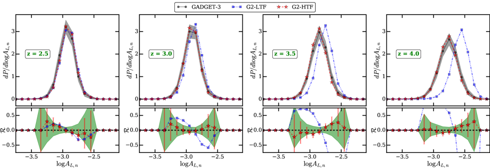
Figure 10: Comparison of wavelet PDF obtained from gadget-3, G2-LTF and G2-HTF models. The symbols and line styles are same as in Fig. 8. The wavelet PDF from G2-HTF model is within 16 percent with that from gadget-3 model while the wavelet PDF from G2-LTF is significantly different at $z\geq 3$ than gadget-3 model.

Table 2: Median wavelet power ($\log A_{L,n}$) in 4 different redshifts bins for the gadget-3, G2-LTF and G2-HTF models. The intervals represent 68 percentile around median.

$z$	gadget-3	G2-LTF	G2-HTF
2.5	$-2.93\pm 0.12$	$-2.91\pm 0.12$	$-2.92\pm 0.12$
3.0	$-2.91\pm 0.12$	$-2.87\pm 0.12$	$-2.91\pm 0.12$
3.5	$-2.85\pm 0.13$	$-2.76\pm 0.12$	$-2.86\pm 0.13$
4.0	$-2.76\pm 0.15$	$-2.57\pm 0.13$	$-2.77\pm 0.14$

The wavelet statistic has been used in the past to constrain $T_{0}$ and $\gamma$ of the IGM (Theuns & Zaroubi, 2000; Theuns et al., 2002; Zaldarriaga, 2002; Lidz et al., 2010; Garzilli et al., 2012). Wavelets have finite support in both real and Fourier space and thus can be used to extract the power at scales of interest. This is necessary because large scales (small $k$) are not sensitive to $T_{0}$, $\gamma$ variation whereas small scales (large $k$) are contaminated by noise and metal lines in observations (Lidz et al., 2010). We use the “Morlet” wavelet, usually a sine (or a cosine) function damped by Gaussian, which has the form

$$\Psi(x)=A\;\exp(-i\>k_{0}\>x)\;\exp\bigg{[}-\frac{x^{2}}{2\>s^{2}_{n}}\bigg{]}$$ (15)

where $s_{n}=35$  km s^-1, and $k_{0}=s_{n}/2\pi$ is the scale over which power is extracted. As shown by Lidz et al. (2010), this scale is sensitive to $T_{0}$ and $\gamma$ variations. $A$ is a normalization constant fixed by,

$$\int\limits_{-\infty}^{\infty}|\Psi(x)|^{2}\;dx=1\;\;\;\;.$$ (16)

The wavelet coefficients are obtained by convolving the  Ly$\alpha$ flux ($F$) with Morlet as,

$$a_{n}(x)=\int\limits_{-\infty}^{\infty}F(x^{\prime})\;\Psi(x-x^{\prime})\;dx^{\prime}$$ (17)

The wavelet power is then given by $A_{n}(x)=|a_{n}(x)|^{2}$. Following Lidz et al. (2010), we smooth the wavelet power on scales of $L=1000$ ${\rm km\;s}^{-1}$ to avoid noisy excursions in wavelet power

$$A_{L,n}(x)=\frac{1}{L}\;\int\limits_{-\infty}^{\infty}\Theta(|x-x^{\prime}|;L/2)\;A_{n}(x^{\prime})\;dx^{\prime}$$ (18)

where $\Theta(|x-x^{\prime}|;L/2)$ is the top-hat filter. It is important to note that wavelet power is anti-correlated with $T_{0}$ i.e., the wavelet power is smaller for higher $T_{0}$ and vice-versa.

Fig. 10 shows the comparison of the PDF of the smoothed wavelet power $(A_{L,n})$ (hereafter wavelet PDF) from the three models. As the TDR parameters $T_{0}$ and $\gamma$ evolve with redshift, the peak and amplitude of the wavelet PDF also evolves accordingly. The bottom panels in Fig. 10 show that the wavelet PDF for G2-HTF model is within sample variance (green shaded region) and within 18 percent (red stars with errorbars) to that from the gadget-3 model at all redshifts. In contrast, the wavelet PDF is systematically shifted to larger values at higher redshifts for the G2-LTF model as compared to the gadget-3 model even though the thermal history parameters are quite similar at those redshifts (see Fig. 4). This can also be seen from Table. 2 where the median wavelet power is consistently larger at higher redshift. Since the distribution is skewed, the errors given in Table. 2 correspond to 68 percentile around the median value. The median wavelet power from G2-HTF model is in good agreement (0.4 percent) with that from gadget-3. However, median wavelet power in G2-LTF model is consistently lower than that from gadget-3 model at higher redshifts ($z\geq 3.5$, difference $\sim 7$ percent). This is because the wavelet scale used in our analysis ($s_{\rm n}=35$  km s^-1) corresponds to $k\sim 0.18\;{\rm s\;km}^{-1}$ shown by magenta dashed vertical line in Fig. 9. At this scale, the G2-LTF FPS has larger power as compared to gadget-3 FPS due to difference in density evolution and thermal history of the particles. Thus corresponding wavelet power is also larger for G2-LTF model as compared to gadget-3 model. Note that the wavelet power is still large in G2-LTF model even if we use a factor $\sim 2$ higher $\Gamma_{\rm HI}$ (corresponding to best fit value for G2-LTF model see section 4.9).

Due to such systematics, the inferred $T_{0}$ from G2-LTF model (or models in which Jeans smoothing effect from thermal history are not accounted for) would be larger at higher redshift and may lead to a misinterpretation of earlier He ii reionization. On the other hand G2-HTF model though approximate in computing the Jeans smoothing does produce consistent results with that from gadget-3. Thus the inferred $T_{0}$ from G2-HTF model doesn’t seem to be skewed by any systematic discussed above.

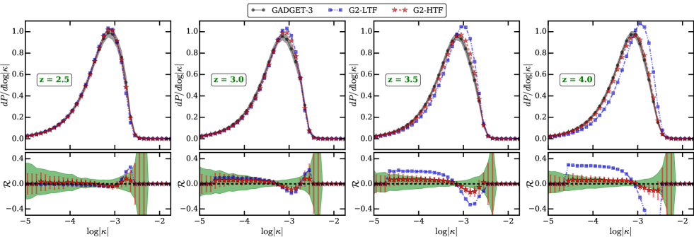
Figure 11: Comparison of curvature PDF obtained from gadget-3, G2-LTF and G2-HTF models. The symbols and line styles are same as in Fig. 8. The curvature PDF from G2-HTF model is within 10 percent with that from gadget-3 model at all redshifts. The sample variances are usually higher than these differences. In contrast, the curvature is systematically larger at higher redshifts in the G2-LTF than in the gadget-3 model (residual is as high as 120 percent).

4.5 Curvature statistics

Table 3: Median curvature in 4 different redshifts bins for the gadget-3, G2-LTF and G2-HTF models.

$z$	gadget-3	G2-LTF	G2-HTF
2.5	$-3.35\pm 0.57$	$-3.35\pm 0.58$	$-3.35\pm 0.58$
3.0	$-3.32\pm 0.60$	$-3.29\pm 0.61$	$-3.31\pm 0.60$
3.5	$-3.29\pm 0.63$	$-3.22\pm 0.65$	$-3.27\pm 0.64$
4.0	$-3.28\pm 0.69$	$-3.17\pm 0.72$	$-3.26\pm 0.70$

Similar to the wavelet analysis, Becker et al. (2011) introduced a curvature statistics to measure the amount of small-scale structure in the  Ly$\alpha$ forest. The curvature $\kappa$ is defined as,

$$\kappa\equiv\frac{F^{\prime\prime}}{[1+(F^{\prime})^{2}]^{3/2}}$$ (19)

where $F^{\prime}$, $F^{\prime\prime}$ is first and second derivative of  Ly$\alpha$ transmitted flux respectively. This statistics is suitable for obtaining the IGM temperature at characteristic overdensity which is found to be an almost one-to-one function of the mean curvature regardless of $\gamma$ (Becker et al., 2011; Boera et al., 2014; Padmanabhan et al., 2014, 2015; Upton Sanderbeck et al., 2016). Following the earlier works, Padmanabhan et al. (2015) have shown that the mean and the percentiles of the curvature distribution function can be used to obtain constraints on the TDR. The comparisons of curvature PDF from three models are shown in Fig. 11. The curvature PDF from G2-HTF model is within 10 percent to that from gadget-3 model at all redshifts. On the other hand, curvature is systematically more at higher redshifts for G2-LTF models than those of gadget-3 models and the residuals are as high as $\sim 120$ percent. The median curvature values are summarized in Table 3. The median curvature in G2-LTF model is systematically higher than that from gadget-3 model at $z=4$. This is because of small scale fluctuations in density field (and hence flux) are larger for the G2-LTF model (see Fig. 9) which affects the curvature measurement. Thus similar to wavelet analysis, the $T_{0}$ inferred from G2-LTF model using curvature statistics would be larger at higher redshifts ($z\geq 3.5$). Whereas $T_{0}$ inferred from G2-HTF model would be consistent with that from gadget-3 model.

4.6 Column Density Distribution function (CDDF)

The next three statistics we will discuss treat the  Ly$\alpha$ forest as a composition of discrete clouds. Each  Ly$\alpha$ line is fitted with multiple Voigt profiles each having 3 free parameters column density (${\rm N_{HI}}$), linewidth ($b$) parameter and line center ($\lambda_{\rm c}$). We used “VoIgt profile Parameter Estimation Routine” (viper) to decompose the  Ly$\alpha$ forest into multi-component Voigt profiles. More details can be found in (Gaikwad et al., 2017b).

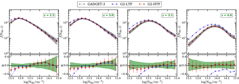
Figure 12: Comparison of CDDF obtained from gadget-3, G2-LTF and G2-HTF models. The symbols and line styles are as in Fig. 8. The incompleteness of the sample is not accounted for in the calculation of CDDF. The CDDF from G2-HTF is consistent within $18$ percent with that from gadget-3 (red stars with errorbars).

The CDDF, $f({\rm N_{HI}},z)$, is a bivariate distribution that describes the number of absorption lines with column density in range  $\log{\rm N_{HI}}$ to  $\log{\rm N_{HI}}$ +  d$\log{\rm N_{HI}}$ and redshift in the range $z$ to $z+dz$. The CDDF is sensitive to $\Gamma_{\rm HI}$ (Schaye, 2001; Shull et al., 2012; Kollmeier et al., 2014; Shull et al., 2015; Gaikwad et al., 2017b; Viel et al., 2016; Gurvich et al., 2017). Fig. 12 shows the comparison of CDDF obtained from gadget-3, G2-LTF and G2-HTF models. We fit the noise free spectra from gadget-3 model and calculate the sample variance as shown by green shaded region in bottom panels. We have not accounted for the incompleteness of the sample in the calculation of redshift path length. This affects the shape of the CDDF at low  $\log{\rm N_{HI}}$ end. The CDDF from G2-HTF models agree within sample variance ($1.25\sigma$) and consistent (within 18 percent) with that from gadget-3 at all redshifts. For  $\log{\rm N_{HI}}$ $>13.5$, the G2-LTF model is consistent within 10 percent at $z\leq 3.5$ except at $z=4$ where the differences are large $\sim 40$ percent. In addition, as expected the G2-LTF model predicts more number of lines at lower column densities i.e.,  $\log{\rm N_{HI}}$ $<13.5$. This is because the features arising from small scale density fluctuations of G2-LTF model (as seen in Fig. 6) is identified and fitted by viper as narrow lines with smaller column densities (for example see the region between $8-9$ cMpc in Fig. 6). However, like other statistics the CDDF from G2-HTF model is in good agreement with that from gadget-3 model.

4.7 Linewidth ($b$ parameter) distribution function

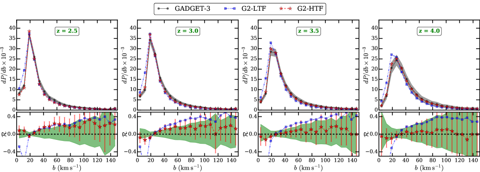
Figure 13: Comparison of $b$ parameter distribution obtained from gadget-3, G2-LTF and G2-HTF models. The symbols and line styles are as in Fig. 8. Each panel is similar to that from Fig. 8 except the comparison is shown for $b$ parameter distrbution from gadget-3 (black circle), G2-LTF (blue squares) and G2-HTF (red stars) models. The $b$ parameter distribution and residuals are plotted from all the lines in sample with relative error in $b$ parameter less than 0.3 (the lines below completeness limit are also included). The green shaded region in the bottom panels show the sample variance on $b$ parameter distribution from gadget-3 model. The $b$ parameter distribution is within $\sim 18$ percent agreement (at $b<60$  km s^-1) with that from the gadget-3.

Table 4: Median $b$ parameter (with 68 percentile interval) in 4 different redshifts bins for the gadget-3, G2-LTF and G2-HTF models.

$z$	gadget-3	G2-LTF	G2-HTF
2.5	25.03${}^{+29.51}_{-9.54}$	22.53${}^{+23.46}_{-9.80}$	22.76${}^{+24.44}_{-8.84}$
3.0	26.61${}^{+30.14}_{-10.02}$	23.22${}^{+22.12}_{-9.65}$	24.69${}^{+27.01}_{-9.58}$
3.5	30.15${}^{+34.69}_{-11.96}$	25.69${}^{+25.23}_{-10.62}$	28.86${}^{+32.21}_{-11.54}$
4.0	35.43${}^{+37.28}_{-15.13}$	29.22${}^{+28.12}_{-12.83}$	34.21${}^{+36.47}_{-14.51}$

The top panels in Fig. 13 show the linewidth distribution, which is sensitive to thermal history, pressure smoothing and unknown turbulent motions in the IGM (Schaye et al., 1999, 2000; McDonald et al., 2001; Davé & Tripp, 2001; Gaikwad et al., 2017b; Viel et al., 2016), from gadget-3 (black circles), G2-LTF (blue squares) and G2-HTF (red stars) models for different redshift bins. The $b$ parameter distribution and residuals plotted in Fig. 13 is calculated from all the lines in sample with relative error in $b$ parameter smaller than 0.5. Again, unlike the G2-LTF model the linewidth distribution from G2-HTF model is consistent (within $18$ percent uncertainty) with that from gadget-3 model at $b<60$  km s^-1. On the other hand residual between G2-LTF and gadget-3 model is large. It is interesting to note that the peak of the $b$ distribution shifts towards larger $b$ values with increasing redshift. This is because the lines tend to be saturated and blended together at higher redshifts. As a result, the fitted $b$ parameter tends to be larger. However, the errors on the fitted $b$ parameters are relatively higher at higher redshifts and hence it is non-trivial to constrain the thermal history of IGM at higher redshifts ($z>3.5$) using line fitting method (Webb & Carswell, 1991; Fernández-Soto et al., 1996). This can also be seen from Table 4 where we have summarize the median $b$ parameters for the $3$ models at 4 different redshifts. The median $b$ increases from $z=2.5$ to $z=4.0$ in all models. The 68 percentile intervals around median are asymmetric because the $b$ distribution is skewed. Within $1\sigma$ errorbars the $b$ distribution from G2-LTF and G2-HTF model is consistent with that from gadget-3 model.

4.8 $b$ versus  $\log{\rm N_{HI}}$ scatter

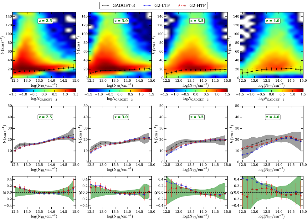
Figure 14: Top panels show the comparison of the $b$ vs  $\log{\rm N_{HI}}$ correlation from gadget-3. The colour scheme indicates density of points in logarithmic units for gadget-3. Middle and bottom panels show comparison of the $b$ vs  $\log{\rm N_{HI}}$ lower envelope for gadget-3, G2-LTF and G2-HTF models. The symbols and line styles are as in Fig. 8. The lower envelopes are obtained by calculating 10^th percentile of $b$ values in  $\log{\rm N_{HI}}$ bin. The lower envelopes for the three model are also shown in top panel.

The top panels in Fig. 14 show the $b$ versus  $\log{\rm N_{HI}}$ scatter for gadget-3 model. The color scheme represents density of points in logarithmic units. One way to assess the goodness of fit is to match the lower-envelope in $b$ versus  $\log{\rm N_{HI}}$ plot. The lower-envelope in the $b$ versus  $\log{\rm N_{HI}}$ plot has been used in the past to constrain the thermal history parameters $T_{0}$ and $\gamma$ (Schaye et al., 1999, 2000; McDonald et al., 2001). Following Garzilli et al. (2015), we obtain the lower-envelope by calculating the $10^{\rm th}$ percentile of $b$ values in  $\log{\rm N_{HI}}$ bin. The middle and bottom panels show the comparison of the lower-envelope obtained from gadget-3, G2-HTF and G2-LTF model. The lower envelope in $b$ versus  $\log{\rm N_{HI}}$ plot from G2-HTF (red stars) is within sample variance and in 18 percent agreement with gadget-3 (black circles). On the other hand, at $z=3.5$ and $4.0$, the lower-envelope from G2-LTF (blue stars) is consistently smaller at  $\log{\rm N_{HI}}$ $<13.5$ than that from gadget-3 model. This can again be attributed to extra absorption line features with smaller  $\log{\rm N_{HI}}$ identified by the viper. Because of the systematically smaller lower-envelop in G2-LTF model at  $\log{\rm N_{HI}}$ $<13.5$, $\gamma$ derived from G2-LTF model would be systematically larger than that from gadget-3 model at $z\geq 3.5$.

To summarize the results presented in sections 4.1–4.8, we find that the  Ly$\alpha$ statistics derived from G2-HTF model are within 20 percent (except for $b$ parameter distribution) to that from gadget-3 model and within the sample variance for a path length of $\sim 1000h^{-1}$ cMpc ($X\sim 5.35$ at $z=3$).

4.9 $\chi^{2}$ analysis

The main motivation of this work is to develop the method to simulate the  Ly$\alpha$ forest in order to efficiently explore the parameter space. Hence, it is important to show the accuracy of the method in recovering the astrophysical parameters. In this section we present the $\chi^{2}$ analysis and show the accuracy of our method in recovering the Hi photoionization rate $\Gamma_{\rm HI}$.

The differences we see between the FPDF and the FPS from different models will have direct consequence in the derived parameter values like $\Gamma_{\rm HI}$. To study this, we treat gadget-3 as the reference model and see how the value of $\Gamma_{\rm HI}$ is recovered when we use the G2-LTF and G2-HTF models. Note that we use the noise (corresponding to SNR=25) added  Ly$\alpha$ transmitted flux in all the models. We vary $\Gamma_{\rm 12}$ in G2-HTF (or G2-LTF) model and calculate the FPDF and FPS. The $\chi^{2}$ between the FPDF / PS calculated from gadget-3 and that from G2-HTF (or G2-LTF) model can be written in the matrix form as (for similar method see Gaikwad et al., 2017a),

$$\chi^{2}_{(\Gamma_{\rm 12})}=[P_{(\Gamma_{\rm 12})}-P_{\rm fid}]\;C^{-1}\;[P_{(\Gamma_{\rm 12})}-P_{\rm fid}]^{\rm T}$$ (20)

where $P_{\rm fid}$ and $P_{(\Gamma_{\rm 12})}$ is flux statistics (either FPDF or PS) from gadget-3 and G2-HTF (or G2-LTF) model respectively. $C$ is the covariance matrix as given in Eq. 13. Note that we use full covariance matrix for $\chi^{2}$ estimation.
$\Gamma_{\rm 12}$ recovery:

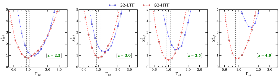
Figure 15: Different panels show the recovery of $\Gamma_{\rm HI}$ for different redshift (given in each panel) using FPDF and FPS stastics. The combined (for FPDF and PS) reduced $\chi^{2}$ as a function of $\Gamma_{\rm 12}$ for G2-LTF (blue squares) and G2-HTF (red stars) model is shown in each panel. gadget-3 is used as the reference model with $\Gamma_{\rm 12}$ = 1. The $\chi^{2}$ is calculated between statistics from gadget-3 and G2-LTF or G2-HTF models (see Table 5). The $1\sigma$ statistical uncertainty on the recovered $\Gamma_{\rm 12}$ for G2-HTF model is indicated by black dashed vertical lines. The above analysis is done for SNR = 25 and for mock sample path length of $1000h^{-1}$ cMpc (corresponding to $X\sim 5.35$ at $z=3$).

The panels in Fig. 15 show reduced $\chi^{2}$ as a function of $\Gamma_{\rm 12}$ from G2-HTF (red stars) and G2-LTF (blue squares) model for four different redshifts. The black dashed vertical lines show the statistical uncertainty in $\Gamma_{\rm 12}$ for G2-HTF model. The $\Gamma_{\rm 12}$ is recovered within $1\sigma$ ($d$$\Gamma_{\rm 12}$ $\sim\pm 0.05$, within $5$ percent accuracy) in G2-HTF model at all redshifts whereas G2-LTF model fails to recover the $\Gamma_{\rm 12}$ within $1\sigma$. The $\Gamma_{\rm 12}$ recovered from G2-LTF model at $z=3.0$ and $z=4.0$ is higher by a factor of 1.7 and 2 respectively. The minimum $\chi^{2}_{\rm dof}$ for G2-HTF model is also close to 1 indicating the goodness-of-fit. Note that the above analysis is done assuming HM12 UVB, SNR = 25 and mock sample path length of $1000h^{-1}$ cMpc (corresponding $X\sim 5.35$ at $z=3$). However, the effect of SNR on $\Gamma_{\rm HI}$ recovery is not significant. To illustrate this, we recover the $\Gamma_{\rm HI}$ at four different redshift bins for SNR varying from 15 to $\infty$ (noise free spectra) as shown in Table 7 of Appendix D. We can see that for wide range of SNR, the $\Gamma_{\rm HI}$ is recovered in the case of G2-HTF model within $5$ percent accuracy. The statistical uncertainty on recovered $\Gamma_{\rm HI}$ is also very similar. This is because, as pointed out earlier, the scatter in FPDF and FPS mainly comes from sample variance. Thus effect of SNR is not important in recovery of $\Gamma_{\rm HI}$. The main conclusion from this study is that the gas pressure is very important while deriving $\Gamma_{\rm HI}$ based on FPDF and FPS. Simple pressure smoothing based on instantaneous temperature and density values can lead to an overestimation of $\Gamma_{\rm HI}$. We show that if we run gadget-2 with higher temperature floor ($T\sim 10^{4}$ K), we are able to recover the correct $\Gamma_{\rm HI}$ within $5$ percent accuracy using our approach.
$\chi^{2}$ analysis for other statistics: We have also calculated the $\chi^{2}$ between G2-HTF and G2-LTF model with gadget-3 as a reference model keeping all other parameters fixed. Table 5 summarizes the reduced $\chi^{2}$ values for different statistics. Note that we calculate the reduced $\chi^{2}$ values for the statistics other than FPDF and FPS using only the diagonal terms of the covariance matrix as the off-diagonal terms are noisy. It is clear from Table 5 that the reduced $\chi^{2}$ is generally less for G2-HTF model as compared to that for G2-LTF model which suggest G2-HTF model is in general better agreement with gadget-3 model. The $\chi^{2}$ analysis for the case of an enhanced UVB is presented in Appendix E where we show that the G2-HTF model is consistent with gadget-3 model for a significantly different thermal history.

Table 5: Reduced $\chi^{2}$ between G2-LTF, G2-HTF model and reference model gadget-3 for different statistics.

	$z=2.5$		$z=3.0$		$z=3.5$		$z=4.0$
Statistics1	G2-LTF	G2-HTF	G2-LTF	G2-HTF	G2-LTF	G2-HTF	G2-LTF	G2-HTF
Density Power spectrum ($\delta$)	0.41	0.98	0.67	0.79	0.82	0.60	1.21	0.58
FPDF	1.26	0.76	1.41	0.80	1.79	0.76	1.87	0.81
FPS	0.50	0.36	0.68	0.25	1.82	0.22	3.23	0.45
Wavelet PDF	0.20	0.42	0.60	0.17	4.46	0.27	12.84	0.74
Curvature PDF	0.30	0.19	1.34	0.49	6.81	0.82	17.07	0.78
CDDF	2.84	1.20	2.85	1.07	4.51	0.47	4.48	0.41
$b$ parameter distribution	4.38	1.04	6.09	0.75	4.56	0.42	2.18	0.73
$b$ vs  $\log{\rm N_{HI}}$ correlation	0.70	0.54	1.27	0.46	1.35	0.44	1.55	0.62

• For a given redshift, all the astrophysical parameters ($T_{0}$, $\gamma$, $\Gamma_{\rm HI}$) are same for G2-LTF, G2-HTF and gadget-3 models. Reduced $\chi^{2}$ is calculated using full covariance matrix for FPDF and FPS. However, for other statistics we used diagonal elements of the covariance matrix as off diagonal elements are noisy.

4.10 Effect of different thermal history

The comparison between different models discussed in sections 4.1-4.9 has been performed for the ionization and heating rates from HM12 UVB model. It is, however, important to validate our method for different UVB models where the thermal history is significantly different from that in the case of the HM12 UVB. In Figs. 19-26, we validate our method (for G2-HTF model) for a UVB models in which $T_{0}$ is increased by a factor of $\sim 2$ while $\gamma$ remains same at all redshifts (see Appendix E for details). We find that the statistics derived from the G2-HTF model is again consistent within 20 percent to that from gadget-3 model for such a different thermal history. Thus for a range of physically motivated photo-heating rates from UVB calculations (such as Khaire & Srianand, 2015a, b), we can easily probe the $T_{0}-\gamma$ parameter space and calculate  Ly$\alpha$ flux in G2-HTF model without performing full gadget-3 simulation. Therefore our method can be a good first step to narrow down the parameter space before confirming the best fit parameter with gadget-3 simulation.

4.11 Computational gain

We now highlight the advantages of using our method for simulating  Ly$\alpha$ forest:

• Efficiency : Table 6 summarizes the CPU time consumption in various parts of the code. Significant fraction of time is spent in evolution of $\Delta$, $v$ and $T$ in both codes. However, unlike gadget-3 we need to evolve $\Delta$, $v$ and $T$ in G2-HTF (or G2-LTF) only once. To vary astrophysical parameters in G2-HTF, we just need to vary UVB in cite. This allows one to probe $T_{0}$ and $\gamma$ parameter space efficiently. For example, the time (per core) required to simulate  Ly$\alpha$ forest for 10 different UVB in gadget-3 is $\sim 67$ days whereas for gadget-2 is $\sim 8$ days.

• Accuracy : We have shown that our method (running gadget-2 with a high temperature floor and post-process using cite) produces statistical distributions that are consistent within sample variance (calculated from mock sample path length of $1000h^{-1}$ cMpc or $X\sim 5.35$ at $z=3$) and within 20 percent to those obtained with gadget-3. In particular, our method is accurate within 5 percent with that from gadget-3 in recovering $\Gamma_{\rm HI}$.

• Flexibility : In addition to HM12, it is straightforward to incorporate other UVB such as Faucher-Giguère et al. (2009); Khaire & Srianand (2015a, b) in cite and evolve the temperature without performing full hydrodynamic simulation. cite can be run in either equilibrium or non-equilibrium ionization evolution mode. It is easy to incorporate cooling due to metals in cite by changing cooling rate tables (Wiersma et al., 2009; Gaikwad et al., 2017a, for similar analysis).

Thus our method (though approximate) is efficient, flexible and sufficiently accurate to explore a large parameter space which otherwise would be more time consuming with self-consistent simulations like gadget-3. However in practice, while constraining astrophysical parameters from observations, we propose to use the method in 3 steps (i) use G2-HTF model to explore large parameter space and obtain the best fit parameters with corresponding statistical uncertainty, (ii) run gadget-3 simulation with best fit parameters (and also for parameters with $1\sigma$ deviation) and (iii) check if the statistics derived from data are consistent with those derived from gadget-3 model with best fit parameters.

Thus our method, while not a substitute for the full hydrodynamical simulation like gadget-3, provide an efficient and reasonable accurate tool to explore a large parameter space which otherwise require large resources and computational time. A possible way to make use this method would be to narrow down the parameter space in the first step before confirming the best fit parameters with a full gadget-3 simulation.

Table 6: Consumption of CPU time (in hours) per core for various tasks of the code for a cosmological run from $z=99$ to $z=2.0$

Step	Descriptiona	gadget-3	G2-HTF
1	$\Delta$, $v$ and $T$ Evolution	156	108
2	cite ($T$ Evolution)b	$-$	3.5
3	Grid calculationc	3.5	4
4	glassd	1	1
-	Total time to run	1605	193
	10 UVB modele	($67$ days)	($8$ days)

• The analysis is done using 256 core on IUCAA PERSEUS cluster.

• cite evolves the temperature of the SPH particles from $z=6.0$ to $z=2.0$. Temperature is evolved internally in gadget-3.

• We used modified smoothing kernel for G2-HTF or G2-LTF as given in Eq. 5. The time is given for 10240 random sightlines through simulation box.

• We apply TDR as given in Eq. 10 for G2-HTF and G2-LTF models. The numbers are given for total 10 $\times$ 2048 simulated  Ly$\alpha$ forest spectra. We splice 5 sightline to cover redshift path length for a single spectra.

• The total time required to run 10 UVB model for gadget-3 is sum of time consumed by steps 1, 3 and 4 (i.e. 160.5 $\times$ 10 hours). Unlike gadget-3, step 1 is performed only once for G2-HTF or G2-LTF models. For different UVB models, we follow step 2-4 in the post-processing stage. Hence the total time required to run 10 UVB model for G2-LTF or G2-HTF model is (108 hours + 8.5 hours $\times$ 10 = 193 hours).

5 Summary

With the advent of high quality observations, an efficient method to simulate the  Ly$\alpha$ forest would be useful for parameter estimation. Current state-of-art simulations like gadget-3, though reproduce observational properties of  Ly$\alpha$ forest very well, are computationally expensive for large parameter space exploration. As part of our ongoing effort, we have developed a post processing module for gadget-2 called “Code for Ionization and Temperature Evolution” (CITE). In Gaikwad et al. (2017a), we have shown that the predictions of our low redshift simulations match well with other existing hydrodynamical simulations and estimated $\Gamma_{\rm HI}$ at $z<0.5$ and associated uncertainties using extensive exploration of the parameter space.

For the resolution used in the above study (gas particle mass $\delta m=1.26\times 10^{7}\>h^{-1}\>{\rm M}_{\sun}$, pixel size $\delta x\sim 48.8h^{-1}$ ckpc), the pressure smoothing of baryons may not be a major issue. However, for studying the high-$z$  Ly$\alpha$ forest one usually uses higher resolution echelle data. When we use appropriate high resolution (gas particle mass $\delta m=1.01\times 10^{5}\>h^{-1}\>{\rm M}_{\sun}$, pixel size $\delta x\sim 9.77h^{-1}$ ckpc) simulation boxes, we notice that the density ($\Delta$) and velocity ($v$) fields are smoother for gadget-3 as compared to those from gadget-2. This is because the temperature and ionization state of the SPH particles in gadget-2 is not calculated self-consistently (photo-heating and radiative cooling terms are not accounted for). In this work we show that by running a gadget-2 simulation with elevated temperature floor (i.e., $T\sim 10^{4}$ K) and using local Jeans smoothing we are able to appreciably overcome the above mentioned shortcomings of our method in the high resolution simulations.

The basic idea is to apply additional smoothing in gadget-2 by a local Jeans length at the epoch of our interest. However, it is well known that the smoothing in gadget-3 is not only decided by the instantaneous density and temperature of the particles but also to some extent by the thermal history of the particles. To understand this, we perform three high resolution simulations (gas particle mass $\delta m=1.01\times 10^{5}\>h^{-1}\>{\rm M}_{\sun}$, pixel size $\delta x\sim 9.77h^{-1}$ ckpc) with same initial conditions (i) G2-LTF: gadget-2 with low temperature ($T\sim 100$ K) floor in which local Jeans length is decided by instantaneous density and temperature and (ii) G2-HTF: gadget-2 with high temperature ($T\sim 10^{4}$ K) floor in which even the unshocked gas is evolved at with a pressure appropriate for a photoionized gas at $T=10^{4}$ K and (iii) gadget-3: a reference model for comparison with G2-LTF and G2-HTF model.

For G2-LTF and G2-HTF models, we first estimate the temperature of SPH particles in gadget-2 using our code cite. We modify the smoothing kernel to account for pressure smoothing and estimated the density, velocity field on grids. We find that the line of sight density and velocity from our method matches well with that from gadget-3. We then compare our method for G2-LTF and G2-HTF models with that from gadget-3 simulation. The main results of our analysis are as follows:

• We obtain the evolution of thermal history parameters $T_{0}$ and $\gamma$ by estimating the temperature of the SPH particles from cite. We show that the redshift evolution of $T_{0}$ and $\gamma$ from G2-HTF and G2-LTF are in very good agreement with that from gadget-3. cite also provides us with enough flexibility to solve the non-equilibrium ionization evolution equation. The $T_{0}$ and $\gamma$ evolution for non-equilibrium case is considerably different ($T_{0}$ is larger by $\sim 60$ percent and $\gamma$ is smaller by 15 percent at $z=3.7$) than that for equilibrium case. We show that the redshift evolution of $T_{0}$ and $\gamma$ for non-equilibrium case from our method is consistent with that from Puchwein et al. (2015, difference less than 2.5 percent).

• We generate the  Ly$\alpha$ forest spectra by shooting random sightlines through simulation box in all the 3 models. The resulting  Ly$\alpha$ forest spectra along sightline are remarkably similar in the G2-HTF and gadget-3 methods. However the  Ly$\alpha$ forest spectra in G2-LTF model show more variation as compared to that from gadget-3. We compare the G2-LTF and G2-HTF with the gadget-3 model using 8 different statistics, namely: (i) 1D density field PS, (ii) FPDF, (iii) FPS, (iv) wavelet PDF, (v) curvature PDF, (vi) column density distribution function, (vii) linewidth distribution and (viii) $b$ vs  $\log{\rm N_{HI}}$ correlation, at four different redshift $z=2.5,3.0,3.5$ and $4.0$. Treating the gadget-3 model as the reference, we demonstrate that the Hi photoionization rate ($\Gamma_{\rm HI}$) can be recovered, using FPDF and FPS statistics, well within $1\sigma$ statistical uncertainty using the G2-HTF model. We find that the G2-HTF model is in general very good agreement (within 20 percent and within $1\sigma$ sample variance calculated from $1000h^{-1}$ cMpc or $X\sim 5.35$ at $z=3$) with gadget-3 model at all redshifts. On the other hand G2-LTF model overestimates the $\Gamma_{\rm HI}$ by a factor of $\sim 2$ at $z\geq 3.5$.

• Using enhanced HM12 photo-heating rates, we obtain a thermal history such that $T_{0}$ is increased by a factor of $\sim 2$. We show that our method for such significantly different thermal history is also consistent (in $1\sigma$) with gadget-3 simulation.

Our method to simulate the  Ly$\alpha$ forest is computationally less expensive, flexible to incorporate changes in UVB, metallicity, non-equilibrium ionization evolution etc. and accurate (in recovering $\Gamma_{\rm HI}$) to within 5 percent. This method can be used in future more effectively to explore $T_{0}$, $\gamma$ and $\Gamma_{\rm HI}$ parameter space and to simultaneously constrain these quantities from observations.

Appendix A Star formation criteria

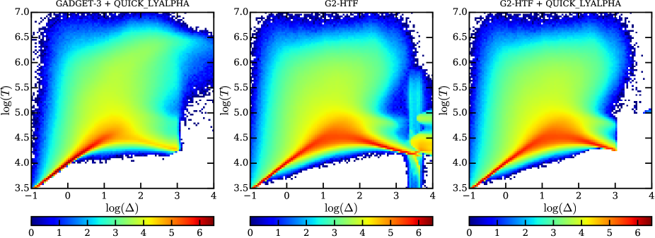
Figure 16: Left, middle and right panel shows the TDR for gadget-3, G2-LTF and G2-LTF with SFR criteria used in QUICK_LYALPHA setting of gadget-3. Particles with $\Delta>1000$ and $T<10^{5}$K are treated as stars and removed from further calculation. The TDR looks remarkably similar for gadget-3 and G2-LTF with QUICK_LYALPHA setting.

To speed up the calculations in gadget-3, we use QUICK_LYALPHA flag that converts gas with $\Delta>1000$ and $T<10^{5}$ K into stars. In order to study its effect on our method, we apply the same criteria to the G2-HTF model. The left, middle and right panels in Fig. 16 show the TDR for gadget-3, G2-HTF model without star formation criteria and G2-HTF model with star formation criteria similar to QUICK_LYALPHA respectively. The TDR for gadget-3 and G2-HTF model with star formation are remarkably similar even at $\Delta>1000$. We also generate  Ly$\alpha$ forest from G2-HTF model with star formation and calculated various  Ly$\alpha$ statistics. We find that the  Ly$\alpha$ statistics are accurate to within 1.8 percent suggesting QUICK_LYALPHA is a good approximation. This is because the particles converted in to stars occupy small volume in the simulation box. The probability that a random sightline (along which  Ly$\alpha$ optical depth is calculated) intersecting such region is small. It should be noted that the results presented in §4 for G2-LTF and G2-HTF do not employ star formation criteria.

Appendix B Convolution of SPH kernel with Gaussian Kernel

In this section, we show that the convolution integral in Eq. 7 can be recast in to an analytical form that is fast and easy to implement on computers. Let $W(r,h)$ be sph kernel and $G(r,\sigma)$ be Gaussian kernel of pressure smoothing. Let $\widetilde{W}(k,h)$ and $\widetilde{G}(k,\sigma)$ be the Fourier transforms of $W(r,h)$ and $G(r,\sigma)$ respectively. The convolution of $W(r,h)$ with $G(r,\sigma)$ is given by,

$$\widetilde{W^{\prime}}(k,h,\sigma) =\widetilde{W}(k,h)\times\widetilde{G}(k,\sigma)$$ (21)

$$W^{\prime}(r,h,\sigma) =\int\frac{{\rm d}^{3}\bm{k}}{(2\pi)^{3}}\;\widetilde{S}(\bm{k},h,\sigma)\;{\rm e}^{\;i\>\bm{k}\cdot\bm{r}}$$

$$W^{\prime}(r,h,\sigma) =\int\frac{{\rm d}^{3}\bm{k}}{(2\pi)^{3}}\;\widetilde{W}(\bm{k},h)\times\widetilde{G}(\bm{k},\sigma)\;{\rm e}^{\;i\>\bm{k}\cdot\bm{r}}$$

Using the convolution theorem,

$$W^{\prime}(r,h,\sigma) =\int\>{\rm d}^{3}\bm{x_{1}}\>W(r_{1},h)\;G(|\bm{r}-\bm{x_{1}}|,\sigma)\;$$ (22)

The sph kernel is given in Eq. 6. The Gaussian kernel in Eq. 8 can be written in following form,

$$G(|\bm{r}-\bm{x_{1}}|,\sigma) =\frac{1}{(2\pi\sigma^{2})^{3/2}}\;\;{\rm exp}\bigg{[}{-\frac{|\bm{r}-\bm{x_{1}}|^{2}}{2\sigma^{2}}}\bigg{]}$$ (23)

$$=\frac{1}{(\pi b^{2})^{3/2}}\;\;{\rm exp}\bigg{[}{-\frac{|\bm{r}-\bm{x_{1}}|^{2}}{b^{2}}}\bigg{]}$$

$$=G_{0}\;\;{\rm exp}\bigg{[}{-\frac{|\bm{r}-\bm{x_{1}}|^{2}}{b^{2}}}\bigg{]}$$

$$=G_{0}\;\;{\rm exp}\bigg{[}{-\frac{(r^{2}+r_{1}^{2}-2\>r\>r_{1}\>\mu)}{b^{2}}}\bigg{]}$$

where, $b=\sqrt{2}\>\sigma$ and $\mu$ is cosine of angle between vector $\bm{r}$ and $\bm{x_{1}}$. The convolution integral can be recast in to the following form,

$$W^{\prime}(r,h,\sigma)=W^{\prime}_{0}\bigg{[}\;\sum\limits_{n=0}^{4}{\rm A}^{+}_{n}\;{\rm I}_{n}\bigg{(}\frac{-r}{b},\frac{h/2-r}{b}\bigg{)}\\ +\;{\rm A}^{-}_{n}\;{\rm I}_{n}\bigg{(}\frac{r}{b},\frac{h/2+r}{b}\bigg{)}+\;{\rm C}^{+}_{n}\;{\rm I}_{n}\bigg{(}\frac{h/2-r}{b},\frac{h-r}{b}\bigg{)}\\ +\;{\rm C}^{-}_{n}\;{\rm I}_{n}\bigg{(}\frac{h/2+r}{b},\frac{h+r}{b}\bigg{)}\bigg{]}$$ (24)

where,

$$W^{\prime}_{0} =\frac{\pi b^{2}\>G_{0}\>W_{0}}{r}$$ (25)

$${\rm A}^{\pm}_{0} =\pm\frac{6\>b\>r^{4}}{h^{3}}\;-\;\frac{6\>b\>r^{3}}{h^{2}}\;+\;b\>r$$

$${\rm A}^{\pm}_{1} =\frac{24\>b^{2}\>r^{3}}{h^{3}}\;\mp\;\frac{18\>b^{2}\>r^{2}}{h^{2}}\;\pm\;b^{2}$$

$${\rm A}^{\pm}_{2} =\pm\frac{36\>b^{3}\>r^{2}}{h^{3}}\;-\;\frac{18\>b^{3}\>r}{h^{2}}$$

$${\rm A}^{\pm}_{3} =\frac{24\>b^{4}\>r}{h^{3}}\;-\;\frac{6\>b^{4}}{h^{2}}$$

$${\rm A}^{\pm}_{4} =\pm\frac{6\>b^{5}}{h^{3}}$$

$${\rm C}^{\pm}_{0} =\mp\frac{2\>b\>r^{4}}{h^{3}}\;+\;\frac{6\>b\>r^{3}}{h^{2}}\;\mp\;\frac{6\>b\>r^{2}}{h}\;+\;2\>b\>r$$ (26)

$${\rm C}^{\pm}_{1} =-\frac{8\>b^{2}\>r^{3}}{h^{3}}\;\pm\;\frac{18\>b^{2}\>r^{2}}{h^{2}}\;-\;\frac{12\>b^{2}\>r}{h}\;\pm\;2\>b^{2}$$

$${\rm C}^{\pm}_{2} =\mp\frac{12\>b^{3}\>r^{2}}{h^{3}}\;+\;\frac{18\>b^{3}\>r}{h^{2}}\;\mp\;\frac{6\>b^{3}}{h}$$

$${\rm C}^{\pm}_{3} =-\frac{8\>b^{4}\>r}{h^{3}}\;\pm\;\frac{6\>b^{4}}{h^{2}}$$

$${\rm C}^{\pm}_{4} =\mp\frac{2\>b^{5}}{h^{3}}$$

$${\rm I}_{n}(l_{1},l_{2}) =\int\limits_{l_{1}}^{l_{2}}\;t^{n}\;{\rm e}^{-t^{2}}\;dt$$ (27)

$${\rm I}_{0}(l_{1},l_{2}) =\frac{\sqrt{\pi}}{2}\;\;\bigg{[}\;{\rm erf~{}}(t)\;\bigg{]}_{l_{1}}^{l_{2}}$$

$${\rm I}_{1}(l_{1},l_{2}) =\bigg{[}\;-\frac{{\rm e}^{-t^{2}}}{2}\;\bigg{]}_{l_{1}}^{l_{2}}$$

$${\rm I}_{2}(l_{1},l_{2}) =\frac{1}{2}\;{\rm I}_{0}(l_{1},l_{2})-\frac{1}{2}\;\bigg{[}t\;{\rm e}^{-t^{2}}\bigg{]}_{l_{1}}^{l_{2}}$$

$${\rm I}_{3}(l_{1},l_{2}) =\;\;\;\;{\rm I}_{1}(l_{1},l_{2})-\frac{1}{2}\;\bigg{[}t^{2}\;{\rm e}^{-t^{2}}\bigg{]}_{l_{1}}^{l_{2}}$$

$${\rm I}_{4}(l_{1},l_{2}) =\frac{3}{2}\;{\rm I}_{2}(l_{1},l_{2})-\frac{1}{2}\;\bigg{[}t^{3}\;{\rm e}^{-t^{2}}\bigg{]}_{l_{1}}^{l_{2}}$$

These integrals involve error function and hence need to be evaluated numerically. To speed up the calculations we used error function approximation of the following form (Abramowitz & Stegun, 1972)

$${\rm erf}(x)=1-(a_{1}\>t+a_{2}\>t^{2}+a_{3}\>t^{3}+a_{4}\>t^{4}+a_{5}\>t^{5})\>{\rm e}^{-x^{2}}+\epsilon(x)$$ (28)

where,

$$t=\frac{1}{1+p\>x}\;\;\;\;{\rm and}$$ (29)

$$|\epsilon(x)|\leq 1.5\times 10^{-7}$$

The small value of $|\epsilon(x)|$ indicates that the uncertainty in error function approximation is negligible. The values of the constants are

$$p =0.3275911 a_{1} =0.254829592$$

$$a_{2} =-0.284496736 a_{3} =1.421413741$$

$$a_{4} =-1.453152027 a_{5} =1.061405429$$

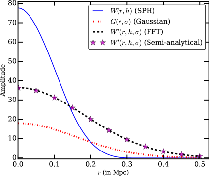
Figure 17: The SPH kernel (see Eq. 6) and Gaussian kernel (Eq. 8) for a particle are shown by blue solid curve and red dashed-dot curve respectively. These two kernels are convolve using FFT based method as shown by black dashed line. Red stars shows our the semi-analytical convolution approximation (given in Eq. 24). Our method of approximation is accurate within 2 percent of FFT based method.

Eq. 7 can also be solved numerically using a 3D FFT based method. However, we find that this method is computationally expensive for large number of particles. Fig. 17 shows a comparison of semi-analytical approximation (red stars, given in Eq. 24) with FFT based method (black dashed curve) for a particle. The SPH kernel and Gaussian kernel for this particle are shown by blue solid curve and red dash dot curves respectively. For visual purpose the Gaussian kernel is rescaled to fit the graph. Our method of approximation for convolution given in Eq. 24 is accurate within 2 percent of FFT based method.

Appendix C Jeans length in G2-HTF model

The G2-LTF and G2-HTF models are gadget-2 simulations with temperature floor $\sim 100$ K and $\sim 10000$ K respectively. For G2-HTF model (high temperature floor) the density field would be smoother as compared to the G2-LTF model (low temperature floor). Hence pressure smoothing scale for G2-HTF model would be smaller than that for G2-LTF. Using Eq. 2, we can quantify the factor by which this pressure smoothing scale is smaller,

$$L \propto T^{\frac{1}{2}\frac{(\gamma-2)}{(\gamma-1)}}$$ (30)

where we have assumed that $T\propto\Delta^{\gamma-1}$ (valid for $\Delta\leq 10$). The median gadget-2 temperature (i.e., before applying cite) in the overdensity range $\Delta\leq 10$ for G2-LTF and G2-HTF model is $T_{\rm{}{G2-LTF}}\sim 4000$ K and $T_{\rm{}{G2-HTF}}\sim 14000$ K respectively. The ratio of pressure smoothing scale in G2-LTF and G2-HTF model is given by (assuming $\gamma\sim 1.6$),

$$\frac{L_{\rm{}{G2-HTF}}}{L_{\rm{}{G2-LTF}}} =\bigg{(}\frac{T_{\rm{}{G2-HTF}}}{T_{\rm{}{G2-LTF}}}\bigg{)}^{\frac{1}{2}\frac{(\gamma-2)}{(\gamma-1)}}\approx 0.66$$ (31)

It is clear from the above expression that if we use $L_{j}$ as pressure smoothing scale for the G2-LTF model in Eq. 5 then we need to use $0.66\times L_{j}$ for the G2-HTF model. Note that we do not modify this value ($0.66$) for a different thermal history corresponding to different UVB (see Appendix E).

Appendix D Effect of different path length and SNR

Effect of path length: The analysis presented in the main paper assumes a default path length for the mock sample as $1000h^{-1}$ cMpc (corresponding to $X\sim 5.35$ at $z=3$). With the advent of surveys like KODIAQ (O’Meara et al., 2015, 2017, $\sim 100$ QSO around $z\sim 2-3.5$), XQ-100 (López et al., 2016), the path length of  Ly$\alpha$ forest covered in QSO absorption spectroscopy is likely to increase by factor of $5$. To study the effect of increase in path length, we generated a mock sample of 100 spectra at redshifts $z=2.5,3.0,3.5,4.0$. We repeated the procedure and generated 100 such mock samples. Thus in all we generated $5\times 100\times 100=50000$ spectra at each redshift (see section 3) and followed the same procedure to calculate $8$ different statistics and the associated uncertainty (see section 4). We find that the $1\sigma$ uncertainty (similar to grey shaded region in Fig.7 to Fig. 14) is decreased by $\sim 12$ percent but it is still dominated by sample variance. The residuals are typically less than 20 percent for G2-HTF model. We are also able to recover the $\Gamma_{\rm HI}$ (using G2-HTF model) within accuracy of $\sim 5$ percent although the reduced $\chi^{2}$ is slightly large ($\sim 1.2$) in this case due to smaller errorbars. Thus increase in path length does not affect the results of the work presented earlier.

Effect of SNR: Table 7 shows the recovery of the $\Gamma_{\rm 12}$ within $1\sigma$ statistical uncertainty from G2-HTF model assuming gadget-3 as a fiducial model (fiducial $\Gamma_{\rm 12}$ $=1$) for different SNR. The path length of mock sample is $1000h^{-1}$ cMpc (see section 3 for details). The values in brackets of Table 7 indicate the reduced $\chi^{2}$ corresponding to best fit $\Gamma_{\rm 12}$. At all redshifts, the G2-HTF model is able to recover the $\Gamma_{\rm 12}$ within $1\sigma$ statistical uncertainty. However, the $\chi^{2}_{\rm dof}$ is large for high SNR. This is because the differences between gadget-3 and G2-HTF model are significant as SNR increases. But even in the case of high SNR, the reduced $\chi^{2}$ is close to 1 indicating the goodness of fit.

Table 7: Recovery of $\Gamma_{\rm 12}$ within statistical uncertainty d $\Gamma_{\rm 12}$ for different SNR for G2-HTF model. The path length of mock sample is $1000h^{-1}$ cMpc ($X\sim 5.35$ at $z=3$). gadget-3 with $\Gamma_{12}=1$ is assumed to be fiducial model.

	The values corresponds to $\Gamma_{\rm 12}$ $\pm$ d$\Gamma_{\rm 12}$ (best fit $\chi^{2}_{\rm dof}$) from G2-HTF model
SNR	$z=2.5$	$z=3.0$	$z=3.5$	$z=4.0$
15	0.97 $\pm$ 0.07 (0.96)	1.02 $\pm$ 0.05 (0.96)	1.00 $\pm$ 0.05 (0.70)	0.98 $\pm$ 0.05 (0.93)
25	0.98 $\pm$ 0.07 (1.09)	1.01 $\pm$ 0.05 (0.96)	1.00 $\pm$ 0.05 (0.84)	0.99 $\pm$ 0.05 (0.98)
35	0.99 $\pm$ 0.07 (1.22)	1.02 $\pm$ 0.05 (1.07)	0.99 $\pm$ 0.05 (0.87)	0.97 $\pm$ 0.04 (1.03)
50	0.98 $\pm$ 0.07 (1.21)	1.01 $\pm$ 0.05 (1.01)	1.01 $\pm$ 0.05 (1.04)	0.97 $\pm$ 0.04 (1.10)
100	1.02 $\pm$ 0.08 (1.33)	1.02 $\pm$ 0.05 (1.11)	1.00 $\pm$ 0.05 (0.95)	0.96 $\pm$ 0.04 (1.30)
Infinite	1.04 $\pm$ 0.07 (1.61)	1.02 $\pm$ 0.05 (1.12)	0.98 $\pm$ 0.05 (1.13)	0.95 $\pm$ 0.04 (1.30)

Appendix E  Ly$\alpha$ flux statistics comparison for different thermal history

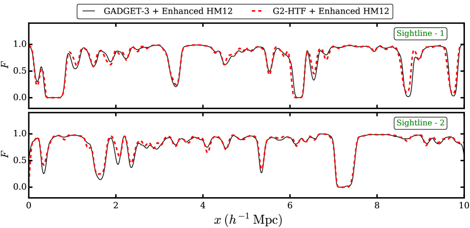
Figure 18: Line of sight comparison of  Ly$\alpha$ flux ($F$) for gadget-3 (black solid line) and G2-HTF (red dashed line) simulation boxes at $z=2.5$ along two different sightlines as shown in top and bottom panels. gadget-3 simulation is performed with an enhanced photo-heating rates (see §4 for details). For G2-HTF model, we used enhanced HM12 photo-heating rates in cite. The  Ly$\alpha$ flux $F$ along the sightline match very well for the two models. The  Ly$\alpha$ flux is not convolved with any LSF and no noise is added to the flux.

In order to explore the effect of difference in thermal history, we follow Becker et al. (2011) and modify the photo-heating rates of species $i=$[H i, He i, He ii] as $\epsilon_{i}=a\times\epsilon_{i}^{\rm HM12}$ where, $\epsilon_{i}^{\rm HM12}$ is HM12 photo-heating rates of specie $i$. We choose $a=2.933$ such that the $T_{0}$ is increased by factor of $\sim 2$ while $\gamma$ remains same at all redshifts. With this updated photo-heating rates we perform a gadget-3 (with QUICK_LYALPHA flag) and G2-HTF simulation with the initial conditions same as described in §2. It is important to emphasize here that we do not perform a gadget-2 simulation again, rather we only modify the HM12 photo-heating rates while running cite in the post-processing stage on the same simulation run earlier. Note that at the initial redshift $z=6$, we use $T_{0}=14543$ K and $\gamma=1.51$ in cite consistent with gadget-3 for enhanced HM12 photo-heating rates at that redshift. Fig. 18 shows comparison of  Ly$\alpha$ flux from gadget-3 and G2-HTF model for enhanced HM12 photo-heating rates. The flux from the two models match very well with each other. We also calculate the line of sight DPS, FPDF, FPS, wavelet PDF, curvature PDF, CDDF, $b$ parameter distribution and $b$ vs  $\log{\rm N_{HI}}$ distribution for these models.

Figs. 19-26 show comparison of different statistics for gadget-3 and G2-HTF model with enhanced HM12 UVB. Since the gas ionized by the enhanced HM12 UVB is at higher temperature (by a factor of $\sim 2$) as compared to the models using HM12 UVB radiation, one would expect to see the differences in the statistics. We notice that the G2-HTF model residuals for FPDF are slightly large in enhanced HM12 UVB ($\sim 20$ percent, see Fig. 20) as compared to those from HM12 UVB ($\sim 15$ percent, see Fig. 8). Similar to HM12 G2-HTF model FPS ($\mathcal{R}\sim 5$ percent, see Fig. 8), we also see the mismatch in enhanced HM12 G2-HTF model ($\mathcal{R}\sim 5$ percent, Fig. 21) at scales in the range $220-650$ ckpc ($k\sim 30-10\>h$  Mpc^-1). The G2-HTF FPS in enhanced HM12 UVB is consistent within $1.6\sigma$ of the sample variance. Wavelets and curvature measurements are anti-correlated with temperature of the IGM. As expected, the comparisons of Fig. 10 with Fig. 22 and Fig. 23 with 11 show that the wavelet PDF and curvature PDF are consistently smaller for enhanced HM12 UVB (higher temperature) respectively. On the other hand the $b$ parameters in enhanced HM12 UVB model (Fig. 25) are consistently larger as compared to that in HM12 UVB model (see Fig.13) at a given redshift. This trend is furthermore clear from Table 8 (compare with Table 2, 3 and 4) where we tabulated the median value of wavelet, curvature and $b$ parameter from gadget-3 and G2-HTF model with enhanced HM12 UVB. The wavelet and curvature PDF in enhanced HM12 UVB for G2-HTF models are in agreement ($1.1\sigma$) with the sample variance. Similarly the CDDF, $b$ parameter distribution and $b$ vs  $\log{\rm N_{HI}}$ lower envelope from G2-HTF model are within sample variance with that from gadget-3 model (see Fig. 24, 25 and 26).

We also calculated the reduced $\chi^{2}$ for different statistics. The reduced $\chi^{2}$ for these statistics are $\sim 0.33,0.67,0.34,0.41,0.59,0.53,0.47$ and $0.58$ respectively. Using this model we are also able to recover $\Gamma_{\rm 12}$ within $1\sigma$ from FPDF and FPS statistics. This shows that G2-HTF model is consistent (within $20$ percent) with gadget-3 model for a significantly different thermal history.

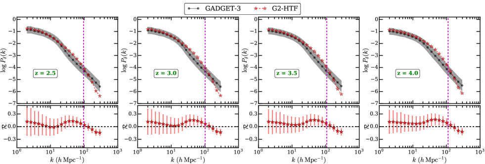
Figure 19: Each panel is same as Fig. 7 except the comparison is shown for gadget-3 and G2-HTF models with enhanced HM12 UVB (see the text for details).

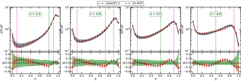
Figure 20: Each panel is same as Fig. 8 except the comparison is shown for gadget-3 and G2-HTF models with enhanced HM12 UVB (see the text for details).

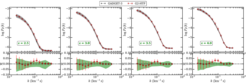
Figure 21: Each panel is same as Fig. 9 except the comparison is shown for gadget-3 and G2-HTF models with enhanced HM12 UVB (see the text for details).

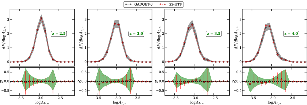
Figure 22: Each panel is same as Fig. 10 except the comparison is shown for gadget-3 and G2-HTF models with enhanced HM12 UVB (see the text for details). Median wavelet values for gadget-3 and G2-HTF model are tabulated in Table. 8.

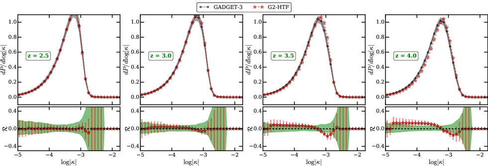
Figure 23: Each panel is same as Fig. 11 except the comparison is shown for gadget-3 and G2-HTF models with enhanced HM12 UVB (see the text for details). Median curvature values for gadget-3 and G2-HTF model are tabulated in Table. 8.

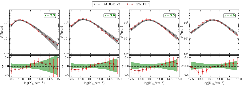
Figure 24: Each panel is same as Fig. 12 except the comparison is shown for gadget-3 and G2-HTF models with enhanced HM12 UVB (see the text for details).

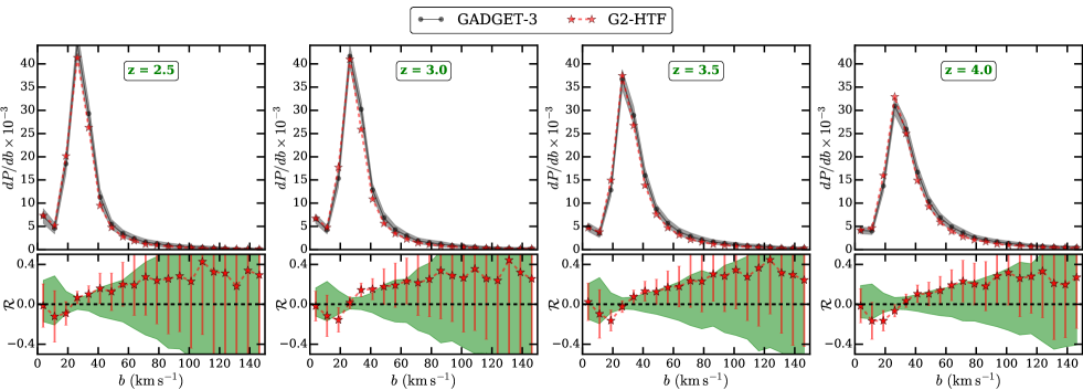
Figure 25: Each panel is same as Fig. 13 except the comparison is shown for gadget-3 and G2-HTF models with enhanced HM12 UVB (see the text for details). Median $b$ parameter values for gadget-3 and G2-HTF model are tabulated in Table. 8.

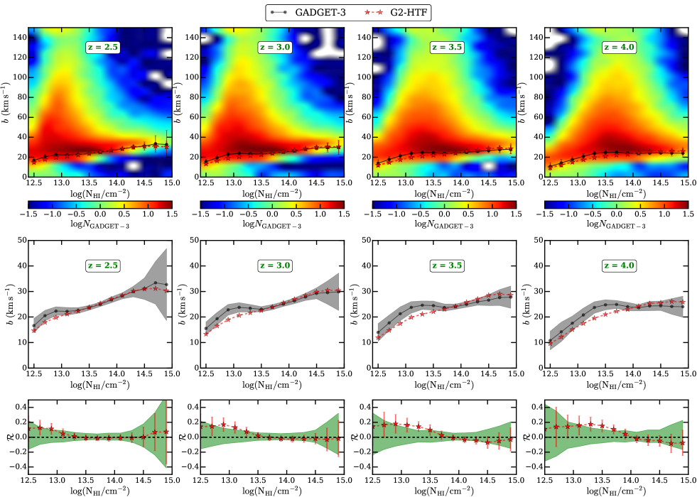
Figure 26: Each panel is same as Fig. 14 except the comparison in middle and bottom panel is shown for gadget-3 and G2-HTF models with enhanced HM12 UVB (see the text for details).

Table 8: Comparison of median wavelet power, curvature and $b$ parameters for the gadget-3 and G2-HTF model with enhanced HM12 UVB. The errorbars correspond to 68 percentile around the median.

Redshift	Median wavelet power		Median curvature		Median $b$ parameter
$z$	gadget-3	G2-HTF	gadget-3	G2-HTF	gadget-3	G2-HTF
2.5	$-2.96\pm 0.13$	$-2.96\pm 0.13$	$-3.43\pm 0.55$	$-3.42\pm 0.57$	32.97${}^{+32.36}_{-12.20}$	29.50${}^{+24.00}_{-11.25}$
3.0	$-3.03\pm 0.14$	$-3.03\pm 0.14$	$-3.41\pm 0.57$	$-3.40\pm 0.58$	34.22${}^{+33.99}_{-12.19}$	30.44${}^{+26.23}_{-11.15}$
3.5	$-3.12\pm 0.15$	$-3.12\pm 0.16$	$-3.39\pm 0.60$	$-3.37\pm 0.61$	36.15${}^{+36.64}_{-12.67}$	32.23${}^{+28.65}_{-11.42}$
4.0	$-3.21\pm 0.16$	$-3.22\pm 0.16$	$-3.39\pm 0.64$	$-3.35\pm 0.66$	36.76${}^{+37.21}_{-13.60}$	33.36${}^{+30.92}_{-12.31}$

References

- Abramowitz & Stegun (1972) Abramowitz M., Stegun I. A., 1972, Handbook of Mathematical Functions
- Arinyo-i-Prats et al. (2015) Arinyo-i-Prats A., Miralda-Escudé J., Viel M., Cen R., 2015, J. Cosmology Astropart. Phys., 12, 017
- Bahcall & Peebles (1969) Bahcall J. N., Peebles P. J. E., 1969, ApJ, 156, L7
- Becker & Bolton (2013) Becker G. D., Bolton J. S., 2013, MNRAS, 436, 1023
- Becker et al. (2011) Becker G. D., Bolton J. S., Haehnelt M. G., Sargent W. L. W., 2011, MNRAS, 410, 1096
- Bi & Davidsen (1997) Bi H., Davidsen A. F., 1997, ApJ, 479, 523
- Bi et al. (1992) Bi H. G., Boerner G., Chu Y., 1992, A&A, 266, 1
- Boera et al. (2014) Boera E., Murphy M. T., Becker G. D., Bolton J. S., 2014, MNRAS, 441, 1916
- Bolton & Haehnelt (2007) Bolton J. S., Haehnelt M. G., 2007, MNRAS, 382, 325
- Bolton et al. (2005) Bolton J. S., Haehnelt M. G., Viel M., Springel V., 2005, MNRAS, 357, 1178
- Bolton et al. (2006) Bolton J. S., Haehnelt M. G., Viel M., Carswell R. F., 2006, MNRAS, 366, 1378
- Bryan et al. (2014) Bryan G. L., et al., 2014, ApJS, 211, 19
- Cen et al. (1994) Cen R., Miralda-Escudé J., Ostriker J. P., Rauch M., 1994, ApJ, 437, L9
- Choudhury et al. (2001) Choudhury T. R., Srianand R., Padmanabhan T., 2001, ApJ, 559, 29
- Cooke et al. (1997) Cooke A. J., Espey B., Carswell R. F., 1997, MNRAS, 284, 552
- Croft et al. (1997) Croft R. A. C., Weinberg D. H., Katz N., Hernquist L., 1997, ApJ, 488, 532
- Croft et al. (1998) Croft R. A. C., Weinberg D. H., Katz N., Hernquist L., 1998, ApJ, 495, 44
- Davé & Tripp (2001) Davé R., Tripp T. M., 2001, ApJ, 553, 528
- Davé et al. (1999) Davé R., Hernquist L., Katz N., Weinberg D. H., 1999, ApJ, 511, 521
- Davé et al. (2010) Davé R., Oppenheimer B. D., Katz N., Kollmeier J. A., Weinberg D. H., 2010, MNRAS, 408, 2051
- Desjacques et al. (2007) Desjacques V., Nusser A., Sheth R. K., 2007, MNRAS, 374, 206
- Doroshkevich & Shandarin (1977) Doroshkevich A. G., Shandarin S. F., 1977, MNRAS, 179, 95P
- Faucher-Giguère et al. (2008) Faucher-Giguère C.-A., Lidz A., Hernquist L., Zaldarriaga M., 2008, ApJ, 682, L9
- Faucher-Giguère et al. (2009) Faucher-Giguère C.-A., Lidz A., Zaldarriaga M., Hernquist L., 2009, ApJ, 703, 1416
- Fernández-Soto et al. (1996) Fernández-Soto A., Lanzetta K. M., Barcons X., Carswell R. F., Webb J. K., Yahil A., 1996, ApJ, 460, L85
- Gaikwad et al. (2017a) Gaikwad P., Khaire V., Choudhury T. R., Srianand R., 2017a, MNRAS, 466, 838
- Gaikwad et al. (2017b) Gaikwad P., Srianand R., Choudhury T. R., Khaire V., 2017b, MNRAS, 467, 3172
- Garzilli et al. (2012) Garzilli A., Bolton J. S., Kim T.-S., Leach S., Viel M., 2012, MNRAS, 424, 1723
- Garzilli et al. (2015) Garzilli A., Theuns T., Schaye J., 2015, MNRAS, 450, 1465
- Gnedin & Hui (1996) Gnedin N. Y., Hui L., 1996, ApJ, 472, L73
- Gnedin & Hui (1998) Gnedin N. Y., Hui L., 1998, MNRAS, 296, 44
- Gurvich et al. (2017) Gurvich A., Burkhart B., Bird S., 2017, ApJ, 835, 175
- Haardt & Madau (2012) Haardt F., Madau P., 2012, ApJ, 746, 125
- Hernquist & Katz (1989) Hernquist L., Katz N., 1989, ApJS, 70, 419
- Hernquist et al. (1996) Hernquist L., Katz N., Weinberg D. H., Miralda-Escudé J., 1996, ApJ, 457, L51
- Hui & Gnedin (1997) Hui L., Gnedin N. Y., 1997, MNRAS, 292, 27
- Jenkins & Ostriker (1991) Jenkins E. B., Ostriker J. P., 1991, ApJ, 376, 33
- Khaire & Srianand (2015a) Khaire V., Srianand R., 2015a, MNRAS, 451, L30
- Khaire & Srianand (2015b) Khaire V., Srianand R., 2015b, ApJ, 805, 33
- Kim et al. (2004) Kim T.-S., Viel M., Haehnelt M. G., Carswell R. F., Cristiani S., 2004, MNRAS, 347, 355
- Kim et al. (2007) Kim T.-S., Bolton J. S., Viel M., Haehnelt M. G., Carswell R. F., 2007, MNRAS, 382, 1657
- Kollmeier et al. (2006) Kollmeier J. A., Miralda-Escudé J., Cen R., Ostriker J. P., 2006, ApJ, 638, 52
- Kollmeier et al. (2014) Kollmeier J. A., et al., 2014, ApJ, 789, L32
- Kulkarni et al. (2015) Kulkarni G., Hennawi J. F., Oñorbe J., Rorai A., Springel V., 2015, ApJ, 812, 30
- Lidz et al. (2010) Lidz A., Faucher-Giguère C.-A., Dall’Aglio A., McQuinn M., Fechner C., Zaldarriaga M., Hernquist L., Dutta S., 2010, ApJ, 718, 199
- López et al. (2016) López S., et al., 2016, A&A, 594, A91
- Lukić et al. (2015) Lukić Z., Stark C. W., Nugent P., White M., Meiksin A. A., Almgren A., 2015, MNRAS, 446, 3697
- McDonald (2003) McDonald P., 2003, ApJ, 585, 34
- McDonald et al. (2000) McDonald P., Miralda-Escudé J., Rauch M., Sargent W. L. W., Barlow T. A., Cen R., Ostriker J. P., 2000, ApJ, 543, 1
- McDonald et al. (2001) McDonald P., Miralda-Escudé J., Rauch M., Sargent W. L. W., Barlow T. A., Cen R., 2001, ApJ, 562, 52
- McDonald et al. (2005) McDonald P., et al., 2005, ApJ, 635, 761
- McDonald et al. (2006) McDonald P., et al., 2006, ApJS, 163, 80
- McGill (1990) McGill C., 1990, MNRAS, 242, 544
- Meiksin & White (2004) Meiksin A., White M., 2004, MNRAS, 350, 1107
- Miralda-Escudé et al. (1996) Miralda-Escudé J., Cen R., Ostriker J. P., Rauch M., 1996, ApJ, 471, 582
- Monaghan (1992) Monaghan J. J., 1992, ARA&A, 30, 543
- Muecket et al. (1996) Muecket J. P., Petitjean P., Kates R. E., Riediger R., 1996, A&A, 308, 17
- Narayanan et al. (2000) Narayanan V. K., Spergel D. N., Davé R., Ma C.-P., 2000, ApJ, 543, L103
- O’Meara et al. (2015) O’Meara J. M., et al., 2015, AJ, 150, 111
- O’Meara et al. (2017) O’Meara J. M., Lehner N., Howk J. C., Prochaska J. X., Fox A. J., Peeples M. S., Tumlinson J., O’Shea B. W., 2017, preprint, (arXiv:1707.07905)
- O’Shea et al. (2005) O’Shea B. W., Nagamine K., Springel V., Hernquist L., Norman M. L., 2005, ApJS, 160, 1
- Padmanabhan et al. (2014) Padmanabhan H., Choudhury T. R., Srianand R., 2014, MNRAS, 443, 3761
- Padmanabhan et al. (2015) Padmanabhan H., Srianand R., Choudhury T. R., 2015, MNRAS, 450, L29
- Palanque-Delabrouille et al. (2015a) Palanque-Delabrouille N., et al., 2015a, J. Cosmology Astropart. Phys., 2, 045
- Palanque-Delabrouille et al. (2015b) Palanque-Delabrouille N., et al., 2015b, J. Cosmology Astropart. Phys., 11, 011
- Peirani et al. (2014) Peirani S., Weinberg D. H., Colombi S., Blaizot J., Dubois Y., Pichon C., 2014, ApJ, 784, 11
- Planck Collaboration et al. (2016) Planck Collaboration et al., 2016, A&A, 594, A13
- Press et al. (1992) Press W. H., Teukolsky S. A., Vetterling W. T., Flannery B. P., 1992, Numerical recipes in FORTRAN. The art of scientific computing
- Puchwein et al. (2015) Puchwein E., Bolton J. S., Haehnelt M. G., Madau P., Becker G. D., Haardt F., 2015, MNRAS, 450, 4081
- Rauch et al. (1997) Rauch M., et al., 1997, ApJ, 489, 7
- Regan et al. (2007) Regan J. A., Haehnelt M. G., Viel M., 2007, MNRAS, 374, 196
- Rollinde et al. (2013) Rollinde E., Theuns T., Schaye J., Pâris I., Petitjean P., 2013, MNRAS, 428, 540
- Schaye (2001) Schaye J., 2001, ApJ, 559, 507
- Schaye et al. (1999) Schaye J., Theuns T., Leonard A., Efstathiou G., 1999, MNRAS, 310, 57
- Schaye et al. (2000) Schaye J., Theuns T., Rauch M., Efstathiou G., Sargent W. L. W., 2000, MNRAS, 318, 817
- Schaye et al. (2010) Schaye J., et al., 2010, MNRAS, 402, 1536
- Scoccimarro et al. (2012) Scoccimarro R., Hui L., Manera M., Chan K. C., 2012, Phys. Rev. D, 85, 083002
- Shull et al. (2012) Shull J. M., Smith B. D., Danforth C. W., 2012, ApJ, 759, 23
- Shull et al. (2015) Shull J. M., Moloney J., Danforth C. W., Tilton E. M., 2015, ApJ, 811, 3
- Smith et al. (2011) Smith B. D., Hallman E. J., Shull J. M., O’Shea B. W., 2011, ApJ, 731, 6
- Sorini et al. (2016) Sorini D., Oñorbe J., Lukić Z., Hennawi J. F., 2016, ApJ, 827, 97
- Springel (2005) Springel V., 2005, MNRAS, 364, 1105
- Springel et al. (2001) Springel V., Yoshida N., White S. D. M., 2001, New Astron., 6, 79
- Theuns & Zaroubi (2000) Theuns T., Zaroubi S., 2000, MNRAS, 317, 989
- Theuns et al. (1998) Theuns T., Leonard A., Efstathiou G., 1998, MNRAS, 297, L49
- Theuns et al. (2002) Theuns T., Zaroubi S., Kim T.-S., Tzanavaris P., Carswell R. F., 2002, MNRAS, 332, 367
- Upton Sanderbeck et al. (2016) Upton Sanderbeck P. R., D’Aloisio A., McQuinn M. J., 2016, MNRAS, 460, 1885
- Viel & Haehnelt (2006) Viel M., Haehnelt M. G., 2006, MNRAS, 365, 231
- Viel et al. (2002) Viel M., Matarrese S., Mo H. J., Theuns T., Haehnelt M. G., 2002, MNRAS, 336, 685
- Viel et al. (2004a) Viel M., Haehnelt M. G., Springel V., 2004a, MNRAS, 354, 684
- Viel et al. (2004b) Viel M., Weller J., Haehnelt M. G., 2004b, MNRAS, 355, L23
- Viel et al. (2005) Viel M., Lesgourgues J., Haehnelt M. G., Matarrese S., Riotto A., 2005, Phys. Rev. D, 71, 063534
- Viel et al. (2009) Viel M., Bolton J. S., Haehnelt M. G., 2009, MNRAS, 399, L39
- Viel et al. (2013a) Viel M., Becker G. D., Bolton J. S., Haehnelt M. G., 2013a, Phys. Rev. D, 88, 043502
- Viel et al. (2013b) Viel M., Schaye J., Booth C. M., 2013b, MNRAS, 429, 1734
- Viel et al. (2016) Viel M., Haehnelt M. G., Bolton J. S., Kim T.-S., Puchwein E., Nasir F., Wakker B. P., 2016, preprint, (arXiv:1610.02046)
- Webb & Carswell (1991) Webb J. K., Carswell R. F., 1991, in Shaver P. A., Wampler E. J., Wolfe A. M., eds, Quasar Absorption Lines. p. 3
- Wiersma et al. (2009) Wiersma R. P. C., Schaye J., Smith B. D., 2009, MNRAS, 393, 99
- Yeche et al. (2017) Yeche C., Palanque-Delabrouille N., . Baur J., du Mas des BourBoux H., 2017, preprint, (arXiv:1702.03314)
- Zaldarriaga (2002) Zaldarriaga M., 2002, ApJ, 564, 153
- Zaldarriaga et al. (2001) Zaldarriaga M., Hui L., Tegmark M., 2001, ApJ, 557, 519
- Zhan et al. (2005) Zhan H., Davé R., Eisenstein D., Katz N., 2005, MNRAS, 363, 1145
- Zhang et al. (1995) Zhang Y., Anninos P., Norman M. L., 1995, ApJ, 453, L57