A Bayesian Filtering Algorithm for Gaussian Mixture Models

Abstract

A Bayesian filtering algorithm is developed for a class of state-space systems that can be modelled via Gaussian mixtures. In general, the exact solution to this filtering problem involves an exponential growth in the number of mixture terms and this is handled here by utilising a Gaussian mixture reduction step after both the time and measurement updates. In addition, a square-root implementation of the unified algorithm is presented and this algorithm is profiled on several simulated systems. This includes the state estimation for two non-linear systems that are strictly outside the class considered in this paper.

1 INTRODUCTION

The problem of estimating the state of a system based on noisy observations of the system outputs has received significant research attention for more than half a century [1]. This attention stems from the fact that state estimation is used in many areas of science and engineering, including—for example—guidance, navigation and control of autonomous vehicles [2], target tracking [3], fault diagnosis [4], system identification [5] and many other related areas.

This research has resulted in many approaches to the state-estimation problem including the much celebrated Kalman filter [6], extended Kalman filter [7], Unscented Kalman filter [8] and Sequential Monte-Carlo (SMC) approaches [9]. Each of these variants exploits different structural elements of the state-space model and each has known strengths and associated weaknesses. For example, if the system is linear and Gaussian, then the Kalman filter is the most obvious choice. On the other hand, if the system is highly non-linear then SMC methods may be the most suitable choice.

In this paper, we consider state estimation for a class of state-space models that can be described by Gaussian mixture models, for both the process and measurement models. This model class captures a broad range of systems including, for example, stochastically switched linear Gaussian systems, systems that exhibit multi-modal state and/or measurement noise, and systems that exhibit long–tailed stochastic behaviour, to name a few. In theory, Gaussian mixtures are suitable for modelling a large class of probability distributions [10].

Inclusion of Gaussian mixtures in the Bayesian filtering framework dates at least back the work in [11], where a mixture was employed to represent the predicted and filtered densities for general non-linear systems. As identified in [11], a significant drawback of this approach is that the number of mixture components can grow rapidly as the filter progresses. Subsequent work in this area has concentrated efforts towards ameliorating this problem by reducing the mixture. This includes approaches based on SMC methods, Expectation Maximisation (EM) clustering, Unscented transforms and many related methods [12, 13, 14, 15]. A common theme among these contributions is that they employ particle resampling techniques to reduce the number of components that need to be tracked. This is either achieved directly by removing highly unlikely components of the mixture, or numerically via resampling algorithms.

Gaussian mixtures are also employed within the area of multiple target tracking problems [3]. Within this field, the methods of Multiple-Hypothesis Kalman Trackers (MHT) and Gaussian Mixture Probability Hypothesis Density filters (GM-PHD) rely on similar ideas presented here, albeit for the target tracking problem [3]. The key idea here is remove unlikely targets from the list of possible targets using a pruning mechanism.

Closely related to these ideas is the independent area of Gaussian mixture model reduction. The recent review in [16] compares several of the main contenders in this field. The methods are compared based on accuracy of the reduced mixture relative to the original one, and the efficiency of each algorithm. The conclusion notes that the Kullback–Leibler reduction method of [17] is both efficient and appears to perform well in terms of accurately reducing the Gaussian mixture.

The contribution of this paper is to unite the GMM state-space model structure together with the Kullback-Leibler reduction algorithm to deliver a new Bayesian filtering algorithm for state estimation of GMM state-space models. An important aspect of this algorithm is the numerically stable and efficient implementation by propagating covariance information in square-root form. This relies on the novel contribution of a square-root form Kullback-Leibler GMM reduction algorithm.

2 PROBLEM DESCRIPTION

Consider a general state-space model expressed via a state transition probability and measurement likelihood

$$x_{t+1} \sim p(x_{t+1}|x_{t}),$$ (1)

$$y_{t} \sim p(y_{t}|x_{t}),$$ (2)

where the state $x_{t}\in\mathbb{R}^{n}$ and the output $y_{t}\in\mathbb{R}^{p}$. The state transition probability distribution (1) and the likelihood (2) may be parameter dependent and may also be time-varying, although these embellishments have been ignored for ease of exposition.

Given a collection of observations $Y_{N}=\{y_{1},\ldots,y_{N}\}$, then the general Bayesian filtering problem can be solved recursively via the well known time and measurement equations

$$p(x_{t}|Y_{t}) =\frac{p(y_{t}|x_{t})\,p(x_{t}|Y_{t-1})}{p(y_{t}|Y_{t-1})},$$ (3)

$$p(x_{t+1}|Y_{t}) =\int p(x_{t+1}|x_{t})\,p(x_{t}|Y_{t})\,dx_{t}.$$ (4)

Solving equations (3)–(4) has attracted enormous attention for many decades and this general approach has been successfully employed across disparate areas of science and engineering. In the general case, the solutions to equations (3) and (4) cannot be expressed in closed form, and this has been the focus of significant research activity. Indeed, this difficulty has led to many approximation methods including the employment of Extended Kalman Filters, Unscented Kalman Filters and Sequential Monte-Carlo (Particle) Filters to name but a few.

In this paper, we restrict our attention to a class of state-space systems that are not as general as (1)–(2), yet—in theory—have the potential to approximate general state-space systems arbitrarily well[10]. More precisely, we will consider state-space systems that can be described by a Gaussian Mixture Model (GMM) in the following manner. The prior is described by

$$p(x_{1})=\sum_{i=1}^{N_{p}}\alpha_{i}\,\mathcal{N}(x_{1};\,\mu_{1}^{i},\,P_{1}^{i}),\quad\sum_{i=1}^{N_{p}}\alpha_{i}=1.$$ (5)

The process model is of the form

$$p(x_{t+1}|x_{t})=\sum_{j=1}^{N_{x}}\beta_{t}^{j}\,\mathcal{N}(x_{t+1};\,A_{t}^{j}x_{t}+u_{t}^{j},\,Q_{t}^{j}),\quad\sum_{j=1}^{N_{x}}\beta_{t}^{j}=1.$$ (6)

The measurement model is of the form

$$p(y_{t}|x_{t})=\sum_{k=1}^{N_{y}}\gamma_{t}^{k}\,\mathcal{N}(y_{t};\,C_{t}^{k}x_{t}+v_{t}^{k},\,R_{t}^{k}),\quad\sum_{k=1}^{N_{y}}\gamma_{t}^{k}=1.$$ (7)

In the above, the form $\mathcal{N}(x;\,\mu,\,P)$ is used to denote a standard multivariate Gaussian distribution. The mean offset terms $u_{t}^{j}$ and $v_{t}^{k}$ allow for the inclusion of input signals or other generated signals that do not depend on $x_{t}$.

The model in (5)–(7) is not as general as (1)–(2). However, the primary advantage of restricting attention to this Gaussian mixture model class is that the time and measurement update equations can be expressed in closed form. Indeed, this fact has already been exploited by many authors dating back to the work of [11]. Therein, the Authors raise a serious issue with this approach, which can be observed by following the recursions in (3)–(4) for just a few steps. Specifically, starting with the prior (5), then the first measurement update can be expressed as

$$p(x_{1}|Y_{1}) =\sum_{i=1}^{Np}\sum_{k=1}^{N_{y}}\alpha_{i}\gamma_{k}\frac{\mathcal{N}(y_{1};C_{1}^{k}x_{1}+v_{1}^{k},R_{1}^{k})\,\mathcal{N}(x_{1};\mu_{1}^{i},P_{1}^{i})}{p(y_{1}|Y_{0})},$$ (8)

and updating this filtered state distribution to the predicted state via (4) results in

$$p(x_{2}|Y_{1}) =\sum_{i=1}^{N_{p}}\sum_{j=1}^{N_{x}}\sum_{k=1}^{N_{y}}\alpha_{i}\beta_{1}^{j}\gamma_{1}^{k}\int f_{1}^{i,j,k}(x_{2},x_{1},Y_{1})\,dx_{1},$$ (9)

where

$$f_{1}^{i,j,k}(x_{2},x_{1},Y_{1}) \triangleq\frac{\mathcal{N}(y_{1};C_{1}^{k}x_{1}+v_{1}^{k},R_{1}^{k})}{p(y_{1}|Y_{0})}$$

$$\quad\times\mathcal{N}(x_{2};A_{1}^{j}x_{1}+u_{1}^{j},Q_{1}^{j})\,\mathcal{N}(x_{1};\mu_{1}^{i},P_{1}^{i}).$$ (10)

Therefore, the predicted state distribution is already a GMM with $N_{p}N_{x}N_{y}$ components. This becomes unmanageable whenever either $N_{x}$ or $N_{y}$ are greater than 1, and the number of measurements $N$ becomes large. For example, if $N_{p}=1$, $N_{x}=1$ and $N_{y}=2$, then a very modest $N=100$ measurements would result in the predicted state density composed of $N_{y}^{100}=2^{100}\approx 10^{30}$ Gaussian components—of the same order as the estimated number of bacterial cells on Earth [18]. Clearly this is not practical and the Authors in [11] suggest that the number of terms should be reduced after each iteration of the filter, but do not provide a suitable mechanism for achieving this.

In the current paper, we adopt the approach of maintaining a prediction and filtering Gaussian mixture and utilise the work in [17] to reduce the mixture at each stage via a Kullback-Leibler discrimination approach. Akin to resampling, this approach compresses the distribution while maintaining the most prominent aspects of the mixture model. This approach will be outlined in the following section.

3 FILTERING ALGORITHM

3.1 A Kullback-Leibler GMM Reduction Method

In this section, we will outline the important aspects of a Kullback-Leibler Gaussian Mixture Model reduction method proposed in [17] and show how this can be utilised within a Bayesian filtering framework in the following subsection. Importantly, we extend the work in [17] in a trivial manner to allow for a reduction of the GMM based on a user-defined threshold, and this has the effect of adapting the mixture to a maximum acceptable loss of information.

The main idea in [17] is to reduce a GMM

$$\pi(x)=\sum_{i=1}^{N}w_{i}\pi_{i}(x),\quad\pi_{i}=\mathcal{N}(x;\mu_{i},P_{i}),\quad\sum_{i=1}^{N}w_{i}=1,$$ (11)

to another mixture model

$$\eta(x)=\sum_{i=1}^{M}v_{i}\eta_{i}(x),\quad\pi_{i}=\mathcal{N}(x;\nu_{i},Q_{i}),\quad\sum_{i=1}^{M}v_{i}=1,$$ (12)

where $1\leq M\leq N$ and in this subsection the variables $x$, $P$ and $Q$ and others are to be treated as general variables and are not meant to represent states and covariance matrices defined elsewhere.

The mechanism proposed in [17] to achieve this reduction is to form a component of $\eta(x)$ by merging two components from $\pi(x)$, that is,

$$\eta_{k}(x)=f(\pi_{i}(x),\pi_{j}(x)).$$ (13)

This is repeated until the desired number of components $M$ is achieved. How to merge these two components from $\pi(x)$ and which two to choose are detailed in [17], but here we present the salient features. In terms of the merging function $f(\cdot,\cdot)$, the Authors in [17] employ the following merge that preserves the first- and second-order moments of the original two components

$$f(\pi_{i}(x),\pi_{j}(x))=w_{ij}\,\mathcal{N}(x;\mu_{ij},P_{ij}),$$ (14)

where

$$w_{ij} =w_{i}+w_{j},$$ (15)

$$\mu_{ij} =w_{i|ij}\mu_{i}+w_{j|ij}\mu_{j},$$ (16)

$$P_{ij} =w_{i|ij}P_{i}+w_{j|ij}P_{j}$$

$$\qquad+w_{i|ij}w_{j|ij}(\mu_{i}-\mu_{j})(\mu_{i}-\mu_{j})^{T},$$ (17)

$$w_{i|ij} =\frac{w_{i}}{w_{i}+w_{j}},$$ (18)

$$w_{j|ij} =\frac{w_{j}}{w_{i}+w_{j}}.$$ (19)

It is possible (see Section IV in [17]) to bound the Kullback-Leibler discrimination between $\eta(x)$ and $\pi(x)$ for each reduction. This is not a bound on the difference between $\eta(x)$ and $\pi(x)$, but provides a bound on the discrimination between the mixtures before and after reduction of a component pair. This bound is denoted $B(i,j)$ and is defined as

$$B(i,j) \triangleq\frac{1}{2}\Bigl{[}w_{ij}\log|P_{ij}|-w_{i}\log|P_{i}|-w_{j}\log|P_{j}|\Bigr{]}.$$ (20)

In the above, we have used the notation $|\cdot|$ to represent the matrix determinant.

The utility of the bound $B(i,j)$ is that we can choose among the possible $i$’s and $j$’s to find the combination that generates the smallest value $B(i,j)$, which therefore represents a bound on the smallest Kullback-Leibler discrimination among the possible components. That is, merging the $(i,j)$ mixture components results in the smallest change to the mixture according to the Kullback-Leibler discrimination bound. Importantly, $B(i,j)=B(j,i)$ and $B(i,i)=0$ so it is only necessary to search $\frac{1}{2}N(N-1)$ combinations—less than half of all possible $(i,j)$ pairs.

Once the minimising $(i,j)$-pair is found, then the corresponding components can be merged and the process can be repeated on the new, reduced, mixture. It is worth noting that this approach is completely deterministic in that the resulting data $\{v_{i},\nu_{i},Q_{i}\}_{i=1}^{M}$ that describes the reduced mixture is only a function the original data $\{w_{i},\mu_{i},P_{i}\}_{i=1}^{N}$ that describes the starting mixture.

In the current paper, we are less concerned with a priori fixing the number $M$ of components in the reduced mixture, and are more concerned with minimising the number of components at each iteration of the filter. To that end, here we will detail an algorithm that continues to merge components until the bound $B(i,j)$ exceeds a given threshold. This may be related back to an acceptable loss of accuracy and, although not explored here, it may be possible to compensate for this decrease in entropy by increasing the corresponding covariance terms. This aside, Algorithm 1 produces a new mixture by successive merging until a threshold in $B(i,j)$ is exceeded, or, a desired minimum number of components is achieved.

Algorithm 1 Kullback-Leibler GMM Reduction

0:  Integers $M_{l}>0$ and $M_{u}>0$ that determine a minimum and maximum, respectively, number of components in the reduced mixture, and a threshold $\lambda>0$, and the initial mixture data $\{w_{i},\mu_{i},P_{i}\}_{i=1}^{N}$.

1:  Set $k=N$ and define a set of integers $S\triangleq\{1,\dotsc,N\}$.

2:  Calculate the bound matrix entries $B(i,j)$ using (20) for $i\in S$ and $j\in S$ noting that $B(i,i)=0$ and $B(i,j)=B(j,i)$.

3:  while $k>M_{u}$ or ($k>M_{l}$ and $\min_{i,j}B(i,j)<\lambda$) do

4:     Find $(i^{\star},j^{\star})=\arg\min_{i,j}B(i,j)$.

5:     Merge components $(i^{\star},j^{\star})$ using (15)–(19) so that the $i^{\star}$’th component data is replaced with

$$\{w_{i^{\star}},\mu_{i^{\star}},P_{i^{\star}}\}\leftarrow\{w_{i^{\star}j^{\star}},\mu_{i^{\star}j^{\star}},P_{i^{\star}j^{\star}}\}.$$ (21)

6:     Remove $j^{\star}$ from the set $S$ so that $S\leftarrow S\setminus j^{\star}$.

7:     Set $k\leftarrow k-1$.

8:     Re-calculate the bound matrix entries $B(i,j)$ using (20) for $i\in S$ and $j\in S$ noting that $B(i,i)=0$ and $B(i,j)=B(j,i)$ and noting that only the $i^{\star}$’th row and column will have changed.

9:  end while

3.2 Filtering Algorithm

In this section we will detail the combination of the Bayesian filtering recursions (3)–(4) for the class of Gaussian mixture state-space models defined in (5)–(7), where the number of components in the filtering and predicted mixtures will be reduced at each stage by utilising Algorithm 1. Recall that the reduction is necessary in order to combat the exponential growth in the number of mixture components.

To this end, assume that we have available a prediction mixture given by

$$p(x_{t}|Y_{t-1}) =\sum_{\ell=1}^{N_{t|t-1}}w_{t|t-1}^{\ell}\mathcal{N}(x_{t};\widehat{x}_{t|t-1}^{\ell},P_{t|t-1}^{\ell}),$$ (22)

$$\qquad\qquad\sum_{\ell=1}^{N_{t|t-1}}w_{t|t-1}^{\ell}=1.$$

Note that the prior (5) is already in this form at $t=1$. Consider the measurement update (3), which can be expressed in the current GMM setting as

$$p(x_{t}|Y_{t}) =\sum_{\ell=1}^{N_{t|t-1}}\sum_{k=1}^{N_{y}}w_{t|t-1}^{\ell}\gamma_{t}^{k}\frac{\mathcal{N}(y_{t};C_{t}^{k}x_{t}+v_{t}^{k},R_{t}^{k})}{p(y_{t}|Y_{t-1})}$$

$$\qquad\qquad\qquad\qquad\times\mathcal{N}(x_{t};\widehat{x}_{t|t-1}^{\ell},P_{t|t-1}^{\ell}).$$ (23)

Due to the linear Gaussian structure, this can be expressed as (see Section III in [11])

$$p(x_{t}|Y_{t}) =\sum_{s=1}^{N_{t|t}}w_{t|t}^{s}\,\mathcal{N}(x_{t};\widehat{x}_{t|t}^{s},P_{t|t}^{s}),\qquad\sum_{s=1}^{N_{t|t}}w_{t|t}^{s}=1,$$ (24)

where for each $k=1,\ldots,N_{y}$ and $\ell=1,\ldots,N_{t|t-1}$ it holds that

$$N_{t|t} =N_{t|t-1}N_{y},$$ (25)

$$s \triangleq N_{y}(\ell-1)+k,$$ (26)

$$\widehat{x}_{t|t}^{s} =\widehat{x}_{t|t-1}^{\ell}+K_{t}^{s}e_{t}^{s},$$ (27)

$$e_{t}^{s} =y_{t}-C_{t}^{k}\widehat{x}_{t|t-1}^{\ell}-v_{t}^{k},$$ (28)

and

$$\Sigma_{t}^{s} =C_{t}^{k}P_{t|t-1}^{\ell}(C_{t}^{k})^{T}+R_{t}^{k},$$ (29)

$$K_{t}^{s} =P_{t|t-1}^{\ell}C_{t}^{k}(\Sigma_{t}^{s})^{-1},$$ (30)

$$P_{t|t}^{s} =P_{t|t-1}^{\ell}-K_{t}^{s}\Sigma_{t}^{s}(K_{t}^{s})^{T},$$ (31)

$$w_{t|t}^{s} =\frac{\bar{w}_{t|t}^{s}}{\sum_{s=1}^{N_{t|t}}\bar{w}_{t|t}^{s}},$$ (32)

$$\bar{w}_{t|t}^{s} =\frac{w_{t|t-1}^{\ell}\gamma_{t}^{k}\exp(-\frac{1}{2}(e_{t}^{s})^{T}(\Sigma_{t}^{s})^{-1}e_{t}^{s})}{(2\pi)^{n/2}|\Sigma_{t}^{s}|^{1/2}}.$$ (33)

With this filtering distribution in place, then we can proceed with the time update (4), which can be expressed as

$$p(x_{t+1}|Y_{t}) =\sum_{s=1}^{N_{t|t}}\sum_{j=1}^{N_{x}}w_{t|t}^{s}\beta_{t}^{j}$$

$$\quad\times\int\mathcal{N}(x_{t+1};A_{t}^{j}x_{t}+u_{t}^{j},Q_{t}^{j})\,\mathcal{N}(x_{t};\widehat{x}_{t|t}^{s},P_{t|t}^{s})\,dx_{t}.$$ (34)

Again, due to the linear Gaussian densities involved, we can express this predicted mixture via

$$p(x_{t+1}|Y_{t}) =\sum_{\ell=1}^{N_{t+1|t}}w_{t+1|t}^{\ell}\,\mathcal{N}(x_{t+1};\widehat{x}_{t+1|t}^{\ell},P_{t+1|t}^{\ell}),$$ (35)

$$\qquad\qquad\sum_{\ell=1}^{N_{t+1|t}}w_{t+1|t}^{\ell}=1,$$

where for each $s=1,\ldots,N_{t|t}$ and $j=1,\ldots,N_{x}$ we have that

$$N_{t+1|t} =N_{t|t}N_{x},$$ (36)

$$\ell \triangleq N_{x}(s-1)+j,$$ (37)

$$\widehat{x}_{t+1|t} =A_{t}^{j}\widehat{x}_{t|t}^{s}+u_{t}^{j},$$ (38)

$$P_{t+1|t} =A_{t}^{j}P_{t|t}(A_{t}^{j})^{T}+Q_{t}^{j},$$ (39)

$$w_{t+1|t}^{\ell} =w_{t|t}^{s}\beta_{t}^{j}.$$ (40)

Therefore, we have arrived back at our initial starting assumption in (22), albeit one time step ahead. Hence, the recursion can repeat.

What remains is to reduce the filtered mixture $p(x_{t}|Y_{t})$ and the predicted mixture $p(x_{t+1}|Y_{t})$ at each iteration in order to avoid exponential growth in computational load. To this end, below we define an algorithm that combines the above filtering recursions with Algorithm 1 to provide a practical Bayesian Filtering algorithm for Gaussian Mixture Model state-space systems.

Algorithm 2 GMM Filter

0:  Integers $M_{fl}>0,M_{fu}>0,M_{pl}>0,M_{pu}>0$ that determine the minimum and maximum number of components in the filtering and prediction mixtures after reduction, and threshold values $\lambda_{f}>0$ and $\lambda_{p}>0$ that represent the filtering and prediction thresholds, respectively, for Algorithm 1.

1:  Set $t=1$ and define the initial prediction mixture at $t=1$ according to the prior (5) so that for each $i=1,\ldots,N_{p}$

$$N_{1|0}\triangleq N_{p},\quad w_{1|0}^{i}\triangleq\alpha_{i},\quad\widehat{x}_{1|0}^{i}\triangleq\mu_{1}^{i},\quad P_{1|0}^{i}\triangleq P_{1}^{i}.$$ (41)

2:  while $k\leq N$ do

3:     Calculate $p(x_{t}|Y_{t})$ according to (24) and (25)–(33).

4:     Replace $p(x_{t}|Y_{t})$ with a reduced mixture using Algorithm 1 with $M_{l}=M_{fl}$ and $M_{u}=M_{fu}$, $\lambda=\lambda_{f}$ and where the mixture data corresponds to $\{w_{t|t}^{s},\widehat{x}_{t|t}^{s},P_{t|t}^{s}\}_{s=1}^{N_{t|t}}$.

5:     Calculate the prediction mixture $p(x_{t+1}|Y_{t})$ according to (35) and (36)–(40).

6:     Replace $p(x_{t+1}|Y_{t})$ using Algorithm 1 with $M_{l}=M_{pl}$ and $M_{u}=M_{pu}$, $\lambda=\lambda_{p}$ and where the mixture data corresponds to $\{w_{t+1|t}^{\ell},\widehat{x}_{t+1|t}^{\ell},P_{t+1|t}^{\ell}\}_{\ell=1}^{N_{t+1|t}}$.

7:  end while

4 NUMERICALLY STABLE IMPLEMENTATION

The above discussion outlines Algorithm 2, which produces estimates of the filtering and prediction mixture densities. The main computational tools employed are those common to Kalman Filtering and those introduced in Algorithm 1 to perform the required mixture reduction.

It is well known [19] that when implementing Kalman Filters, care should be taken in ensuring that the covariance matrices remain positive definite and symmetric. Unfortunately, the equations in (25)–(33) and (36)–(40) are not guaranteed to maintain this requirement if implemented naively. To circumvent this problem, we have employed a square-root version of the filtering recursions.

We present the essential idea here in order to help explain a square-root implementation of Algorithm 1 that relies on the mixture being provided in square-root form. To this end, it is assumed that we have access to square-root versions of the covariance matrices

$$P_{1}^{i} =(P_{1}^{i})^{T/2}(P_{1}^{i})^{1/2},$$ (42)

$$Q_{t}^{j} =(Q_{t}^{j})^{T/2}(Q_{t}^{j})^{1/2},$$ (43)

$$R_{t}^{k} =(R_{t}^{k})^{T/2}(R_{t}^{k})^{1/2}.$$ (44)

The measurement update equations (25)–(33) can then be calculated by employing a QR factorisation as follows

$$\begin{bmatrix}\mathcal{R}_{11}^{s}&\mathcal{R}_{12}^{s}\\ 0&\mathcal{R}_{22}^{s}\end{bmatrix} \triangleq\mathcal{Q}^{s}\begin{bmatrix}(R_{t}^{k})^{1/2}&0\\ (P_{t|t-1}^{\ell})^{1/2}(C_{t}^{k})^{T}&(P_{t|t-1}^{\ell})^{1/2}\end{bmatrix}.$$ (45)

In the above $\mathcal{Q}^{s}$ is an orthonormal matrix and $\mathcal{R}_{11}^{s}$ and $\mathcal{R}_{22}^{s}$ are upper triangular matrices. Note that we have dropped the time reference from these matrices for ease of exposition. This then allows for the computation of the remaining terms via

$$(\Sigma_{t}^{s})^{1/2} =\mathcal{R}_{11}^{s},$$ (46)

$$(P_{t|t}^{s})^{1/2} =\mathcal{R}_{22}^{s},$$ (47)

$$\tilde{e}_{t} =(\mathcal{R}_{11}^{s})^{-T}\left(y_{t}-C_{t}^{k}\widehat{x}_{t|t-1}^{\ell}-v_{t}^{k}\right),$$ (48)

$$\widehat{x}_{t|t}^{s} =\widehat{x}_{t|t-1}^{\ell}+(\mathcal{R}_{12}^{s})^{T}\tilde{e}_{t}^{s},$$ (49)

and the weights can be calculated via

$$w_{t|t}^{s} =\frac{\bar{w}_{t|t}^{s}}{\sum_{s=1}^{N_{t|t}}\bar{w}_{t|t}^{s}},$$ (50)

$$\bar{w}_{t|t}^{s} =\frac{w_{t|t-1}^{\ell}\gamma_{t}^{k}\exp(-\frac{1}{2}(\tilde{e}_{t}^{s})^{T}\tilde{e}_{t}^{s})}{(2\pi)^{n/2}\sigma_{t}^{s}},$$ (51)

$$\sigma_{t}^{s} \triangleq\left(\prod_{i=1}^{p}|\Sigma_{t}^{s}(i,i)|^{2}\right)^{1/2}.$$ (52)

Similar arguments can be employed in the prediction step with

$$\begin{bmatrix}\bar{\mathcal{R}}^{\ell}\\ 0\end{bmatrix} \triangleq\bar{\mathcal{Q}}^{\ell}\begin{bmatrix}(P_{t|t}^{s})^{1/2}(A_{t}^{j})^{T}\\ (Q_{t}^{j})^{1/2}\end{bmatrix},$$ (53)

$$(P_{t+1|t}^{\ell})^{1/2} =\bar{\mathcal{R}}^{\ell}.$$ (54)

The remaining prediction equations in (36)–(40) are unchanged.

Therefore, we can compute all the required filtering and prediction covariances in square-root form. Aside from the numerical stability that this brings, we can also exploit the square-root form in Algorithm 1. Specifically, referring to the steps in Algorithm 1, it is important that we can compute the bound $B(i,j)$ efficiently and robustly. To this end, note that according to (15)–(19), if the covariance matrices $\{P_{i},P_{j}\}$ are provided in square-root form then we can compute the following QR factorisation

$$\begin{bmatrix}\tilde{\mathcal{R}}\\ 0\end{bmatrix} =\tilde{\mathcal{Q}}\begin{bmatrix}\sqrt{w_{i|ij}}P_{i}^{1/2}\\ \sqrt{w_{j|ij}}P_{j}^{1/2}\\ \sqrt{w_{i|ij}w_{j|ij}}(\mu_{i}-\mu_{j})^{T}\end{bmatrix},$$ (55)

so that

$$\tilde{\mathcal{R}}^{T}\tilde{\mathcal{R}} =\begin{bmatrix}\sqrt{w_{i|ij}}P_{i}^{1/2}\\ \sqrt{w_{j|ij}}P_{j}^{1/2}\\ \sqrt{w_{i|ij}w_{j|ij}}(\mu_{i}-\mu_{j})^{T}\end{bmatrix}^{T}\begin{bmatrix}\sqrt{w_{i|ij}}P_{i}^{1/2}\\ \sqrt{w_{j|ij}}P_{j}^{1/2}\\ \sqrt{w_{i|ij}w_{j|ij}}(\mu_{i}-\mu_{j})^{T}\end{bmatrix}$$

$$=w_{i|ij}P_{i}^{T/2}P_{i}+w_{j|ij}P_{j}^{T/2}P_{j}^{1/2}$$

$$\qquad\qquad+w_{i|ij}w_{j|ij}(\mu_{i}-\mu_{j})(\mu_{i}-\mu_{j})^{T}$$

$$=P_{ij}.$$ (56)

Therefore,

$$P_{ij}^{1/2} =\tilde{\mathcal{R}}$$ (57)

is a square-root factor for the merged component. In addition, the bound $B(i,j)$ can be readily calculated by exploiting the fact that for any upper triangular matrix $A\in\mathbb{R}^{m\times m}$

$$\log\left|A^{T}A\right|=2\sum_{i=1}^{m}\log|A(i,i)|$$ (58)

to deliver

$$B(i,j) =\sum_{i=1}^{n}w_{ij}\log|P_{ij}^{1/2}(i,i)|-w_{i}\log|P_{i}^{1/2}|-w_{j}\log|P_{j}^{1/2}|.$$ (59)

Therefore, we have shown that the square-root form of the Kalman filter covariance matrices will be maintained after calling the mixture reduction algorithm by employing (55) and (57). We have further shown how to readily compute $B(i,j)$ that exploits this square-root form.

The QR factorisation involved in (55) can also exploit the special sparse structure arising from two stacked upper triangular matrices and one row vector. This feature has been exploited in our implementation, but not detailed here further.

5 EXAMPLES

In this section, we present a collection of examples that profile the proposed Algorithm 2, henceforth referred to as the GMMF approach. We move from a simple linear state-space model with additive Gaussian noise, through to a non-linear and time-varying system that falls outside the modelling assumptions in this paper.

5.1 Linear State-Space Model

In this example, we profile Algorithm 2 on a well known and studied problem of filtering for linear state-space systems with additive Gaussian noise on both the state and measurements. Clearly this falls within our model assumptions (5)–(7) and our purpose here is to observe that even if we deliberately start with more mixture components in the prior $p(x_{1})$ than are strictly necessary, the algorithm will very quickly reduce the number of mixture terms in both the predicted and filtered densities.

To this end, consider the state-space model

$$x_{t+1} =\begin{bmatrix}1&0.01\\ 0&1\end{bmatrix}x_{t}+u_{t}+w_{t},$$ (60)

$$y_{t} =\begin{bmatrix}1&0\end{bmatrix}x_{t}+e_{t},$$ (61)

where the input was chosen as $u_{t}=\begin{bmatrix}0&1\end{bmatrix}^{T}\bar{u}_{t}$ with $\bar{u}_{t}\sim\mathcal{N}(0,0.04)$ and

$$x_{1}\sim\mathcal{N}(0,1),\quad w_{t}\sim\mathcal{N}(0,0.01),\quad e_{t}\sim\mathcal{N}(0,0.1),$$ (62)

We simulated $N=100$ samples from the system and then ran both a Kalman Filter and the GMMF method according to Algorithm 2. The predicted mean of the first state is shown in Figure 1. Notice that the GMMF predicted mean initially differs from the Kalman predicted mean. This was a deliberate choice where the GMMF was initialised with an incorrect prior, as depicted in Figure 2(a). This was generated by choosing $25$ components in the prior that were evenly spaced between $(-10,10)$ in both states.

The purpose here is to demonstrate that the GMMF approach can quickly converge to the correct number of modes and correct for the model mismatch. Indeed, after just $t=7$ steps, the GMMF algorithm had converged to one mixture component in both the predicted and filtered mixtures. The convergence of the predicted PDFs can be observed in Figure 2 as time progresses.

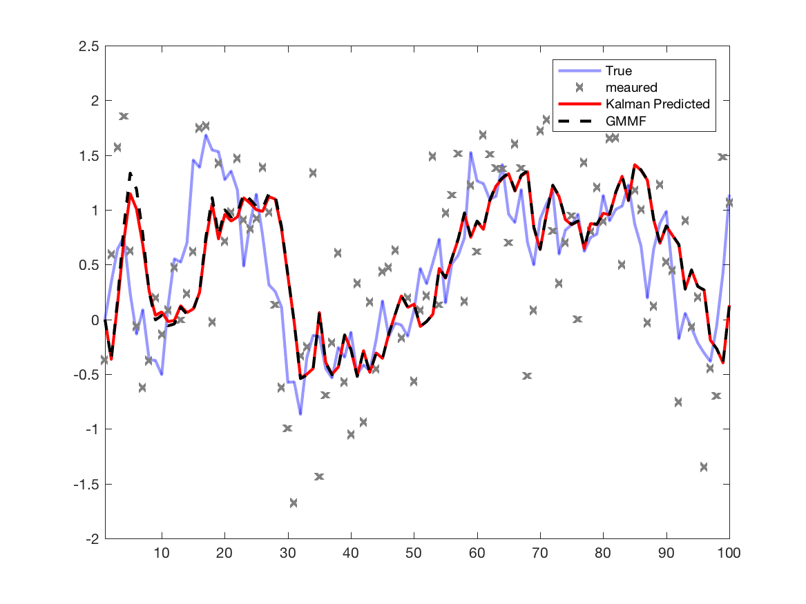
Figure 1: Plot of the predicted mean for the first state from both the Kalman Filter (red) and GMM Filter (dashed black) against the true state (solid blue). Measurements are indicated as crosses.

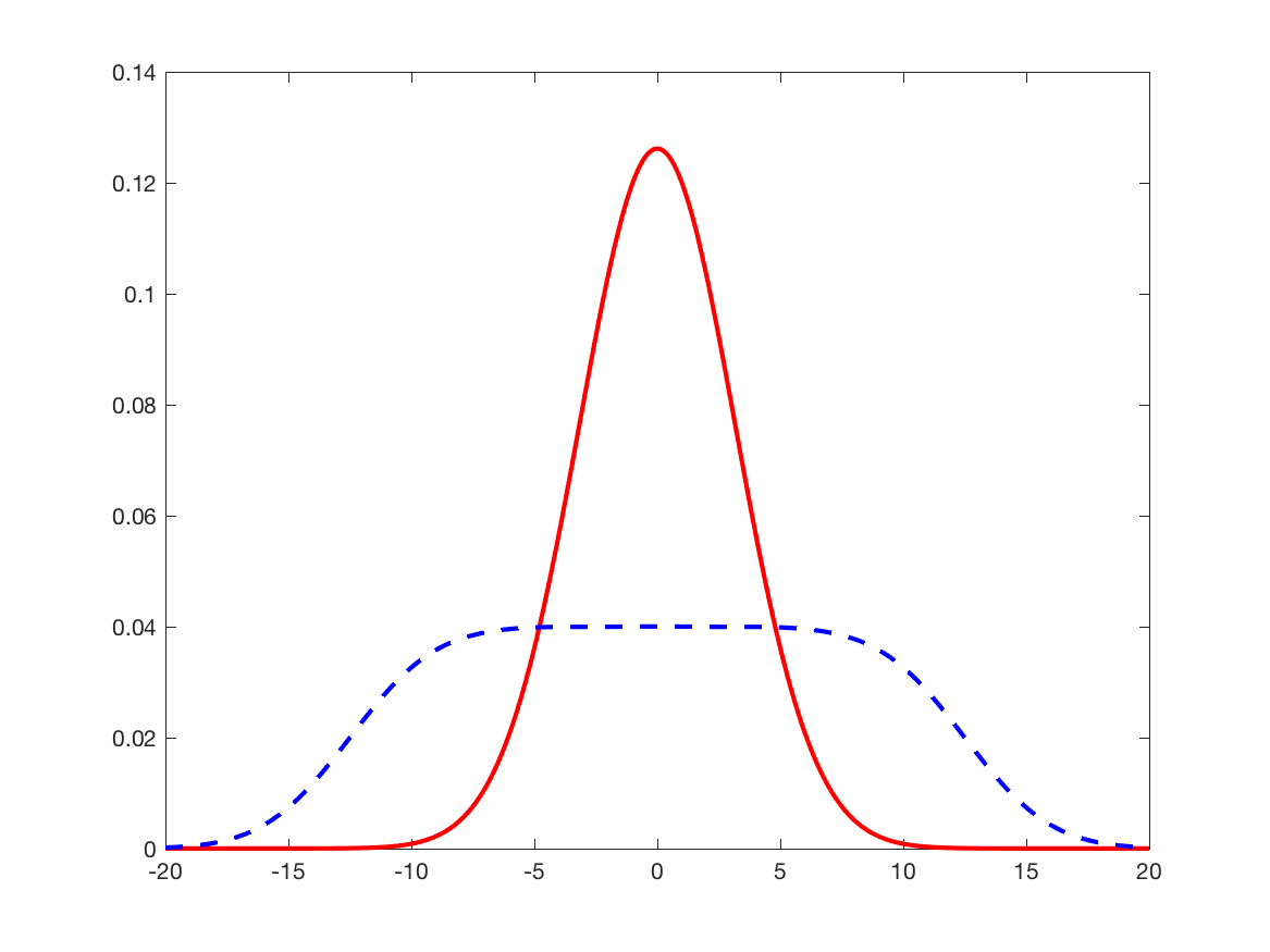
(a) Time $t=1$.

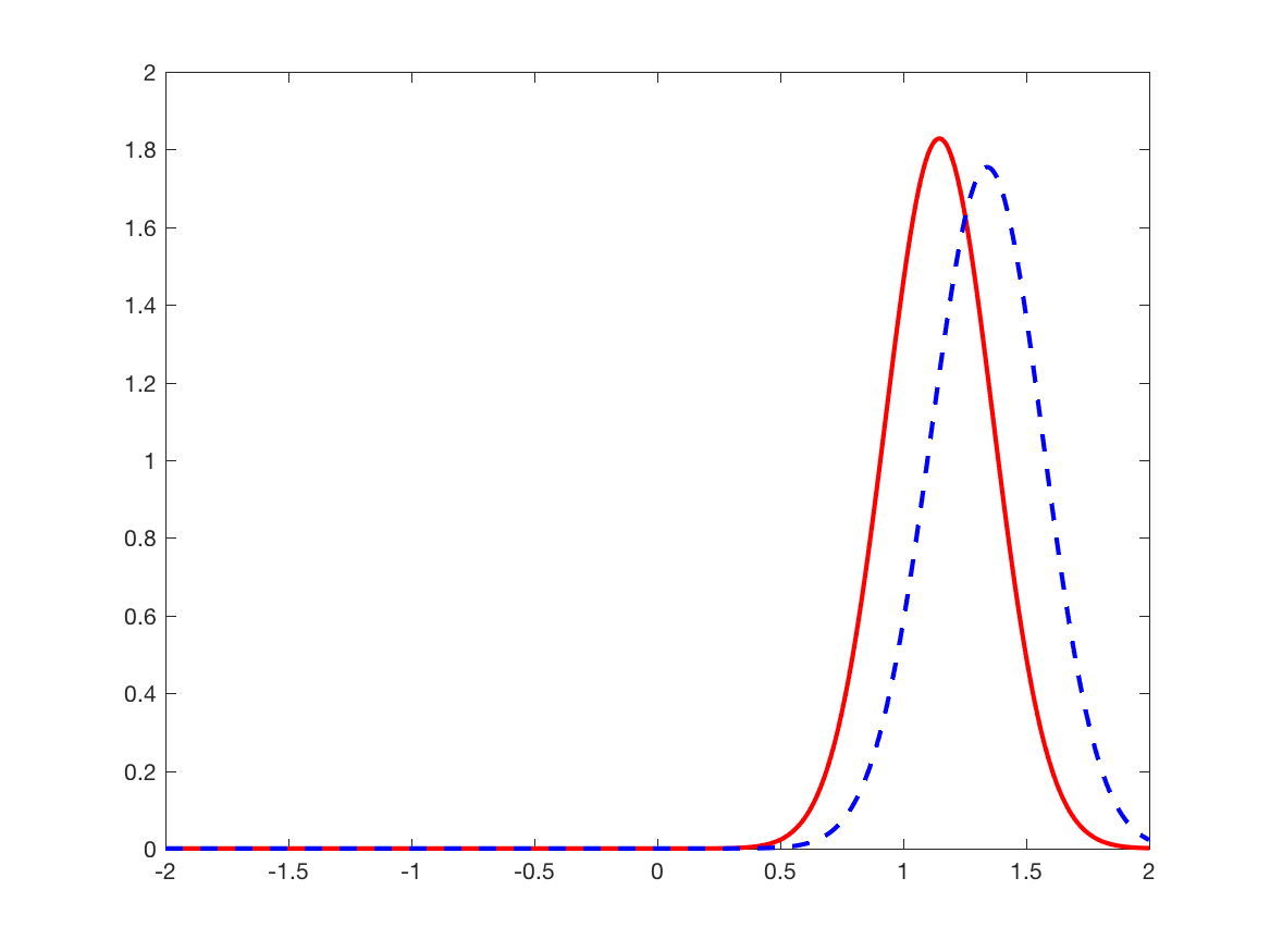
(b) Time $t=5$.

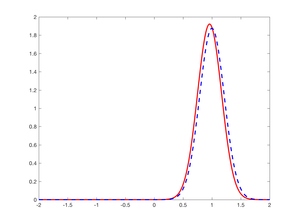
(c) Time $t=20$.

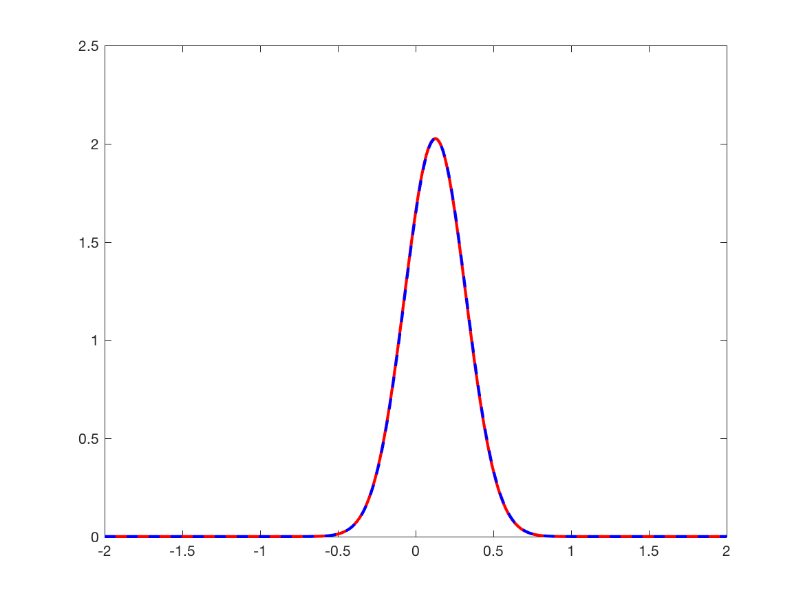
(d) Time $t=100$.

Figure 2: Predicted state densities for different times. Kalman predicted (blue solid) and GMM predicted (red solid).

5.2 Gaussian Mixture Model

In this example, we are interested in profiling the GMMF algorithm for a model that satisfies the assumptions (5)–(7), and yet is not easily amenable to Extended Kalman filtering or Unscented Kalman filtering. Specifically, consider the following GMM state process model with

$$N_{p} =1, \mu_{1} =0, P_{1} =I_{2\times 2},$$

$$N_{x} =2, A^{1} =\begin{bmatrix}1&0.1\\ 0&1\end{bmatrix}, A^{2} =\begin{bmatrix}0.1&0.01\\ 0&0.1\end{bmatrix},$$

$$Q^{1} =0.1^{2}I_{2\times 2}, Q^{2} =0.003^{2}I_{2\times 2},$$

$$\beta^{1} =0.99, \beta^{2} =0.01, u_{t}^{1} =u_{t}^{2}=\begin{bmatrix}\sin(4\pi t/N)\\ 0\end{bmatrix},$$

and where the measurement model is described by

$$N_{y} =2,\quad C^{1}=\begin{bmatrix}1&0\end{bmatrix},\quad C^{2}=\begin{bmatrix}1&0\end{bmatrix},$$

$$v_{t}^{1} =12.5,\quad v_{t}^{2}=-12.5,$$

$$R^{1} =0.1,\quad R^{2}=0.1,\quad\gamma^{1}=0.1,\quad\gamma^{2}=0.9.$$

We simulated $N=200$ samples from this system and used the GMMF method to estimate the state distribution. Figure 3 shows the predicted mean of the first state. For comparison, we also ran a Kalman filter for the most likely model (according to the weight $\beta^{1},\beta^{2},\gamma^{1},\gamma^{2}$). Note that when the modelling assumption is correct, e.g., from $t=100$ to $t=130$, the Kalman mean aligns very well with the GMMF mean as expected.

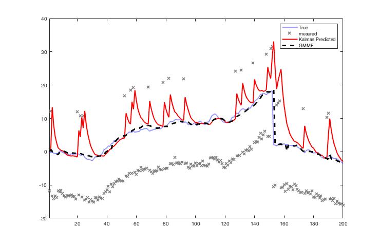
Figure 3: Plot of the predicted mean for the first state from both the Kalman Filter (red) and GMM Filter (dashed black) against the true state (solid blue). Measurements are indicated as crosses.

5.3 Bi-modal Filtered Density Model

In this example, we demonstrate the GMMF algorithm on a model that, due to its measurement equation, has a bi-modal filtered density. The prior and process models satisfy assumptions (5) and (6). Specifically, consider the following GMM state process model:

$$N_{p} =50,\quad\mu_{1}^{i}=-10+(i-1)\frac{20}{49},\quad P_{1}^{i}=0.1,$$ (63)

$$N_{x} =1,\quad A_{1}=1,\quad u_{t}^{1}=5\cos(t_{k}),$$ (64)

$$Q_{1} =0.01,\quad\beta_{1}=1.$$ (65)

Here, however, we use a nonlinear measurement model that does not strictly satisfy the structural assumption in (7). Specifically, the measurement model is of the form

$$y_{k}=h(x_{t})+e_{k},\quad h(x_{t})=x_{k}^{2},\quad e_{k}\sim\mathcal{N}(0,25).$$ (66)

This particular measurement model was chosen to create ambiguity in the filtered state between positive and negative values.

The nonlinear measurement model can be dealt with in the GMMF framework by considering the Laplace approximation of the function for each mixture component. In this case, the measurement model for each component becomes

$$C^{k,\ell}_{t} =\frac{\partial h(x)}{\partial x}\Bigr{|}_{x=\hat{x}_{t|t-1}^{\ell}},\quad v_{t}^{k,\ell}=h(\hat{x}_{t|t-1}^{\ell})-C^{k,\ell}_{t}\hat{x}^{\ell}_{t|t-1}.$$ (67)

This approximates the filtered density in a similar way to a first-order extended Kalman filter. In cases where the mixture components have high variance, the approximation may be poor. In this case, we are able to represent the prediction mixture by a greater number of components than in (9) by splitting each component of the mixture into $N_{s}$ components. Note that the GMM model class easily accommodates this splitting process.

We simulated $N=100$ input/output samples from this system, and ran both the GMMF method and a Sequential Monte-Carlo (SMC) method to estimate the state distribution. The filtered state densities from the GMMF estimator are shown in Figure 4. The predicted and filtered densities at various times are shown in Figure 5. The GMMF was initialised with a prior of $50$ components evenly spaced between $(-10,10)$. Figure 5(a) shows that the GMMF and SMC generated densities are closely matched in this case, despite the GMMF approach using no more than $35$ components in the filtering mixture after the very first filtering step.

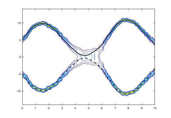
Figure 4: The filtered state density as predicted by the GMMF (contour), against the true state (solid black), and the true state mirrored about $x=0$ (dashed black).

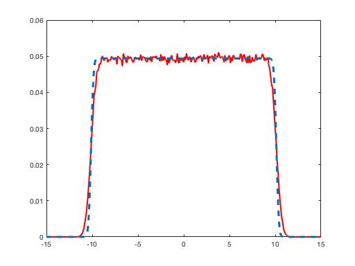
(a) Predicated, Time $t=0.1$.

(b) Filtered, Time $t=0.1$.

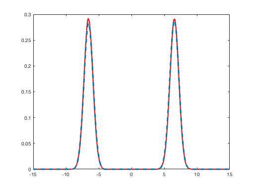
(c) Predicted, Time $t=3$.

(d) Filtered, Time $t=3$.

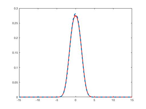
(e) Predicted, Time $t=5$.

(f) Filtered, Time $t=5$.

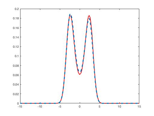
(g) Predicted, Time $t=6$.

(h) Filtered, Time $t=6$.

Figure 5: The predicted and filtered state densities. In each case, the GMMF density (blue) is compared against the density from a SMC method (red).

5.4 Non-linear and Time Varying Model

In this example, we demonstrate the GMMF algorithm on a model that has both a nonlinear process and measurement model. The purpose here is to show that the GMMF filter has potential utlity for cases where the model strictly violates the structural assumptions (5)–(7). The chosen model has received significant attention due it being recognised as a difficult state estimation problem [20, 21]. The process and measurement equations are given by

$$x_{t+1} =f(x_{t})+w_{t},\quad f(x_{t})=ax_{t}+b\frac{x_{t}}{1+x_{t}^{2}}+c\cos(1.2t)$$

$$y_{t} =h(x_{t})+v_{t},\quad h(x_{t})=dx_{t}^{2},$$

where $w_{t}\sim\mathcal{N}(0,1)$ and $e_{t}\sim\mathcal{N}(0,1)$, and the parameter values used are

$$a=0.5,\quad b=25,\quad c=8,\quad d=0.05.$$

As in Section 5.3, the non-linearities are dealt with by taking the Laplace approximations about the mean of each mixture component via

$$A^{j,s}_{t} =\frac{\partial f(x)}{\partial x}\Bigr{|}_{x=\hat{x}_{t|t}^{s}},\quad u_{t}^{j,s}=f(\hat{x}_{t|t}^{s})-A^{j,s}_{t}\hat{x}^{s}_{t|t},$$

$$C^{k,\ell}_{t} =\frac{\partial h(x)}{\partial x}\Bigr{|}_{x=\hat{x}_{t|t-1}^{\ell}},\quad v_{t}^{k,\ell}=h(\hat{x}_{t|t-1}^{\ell})-C^{k,\ell}_{t}\hat{x}^{\ell}_{t|t-1}.$$

In order to improve the approximation of the PDFs given by the prediction and measurement steps, we represent the prediction and filtering densities by a greater number of components than given by (9) and (2), respectively. As in Section 5.3, this is achieved by splitting each mixture component into $N_{s}$ components.

We simulated $N=100$ input/output samples from the system and ran both the GMMF algorithm and, for comparison, a Sequential Monte-Carlo method to estimate the state distributions. Figure 6 shows the predicted mean of the state. The predicted and filtered state densities are shown in Figure 7 for a selection of time samples, where we note the close match between these densities.

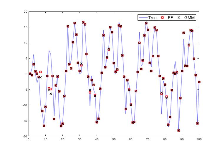
Figure 6: Plot of the predicted state mean from both the GMM Filter (red crosses) and the Particle filter (green squares) against the true state (solid blue).

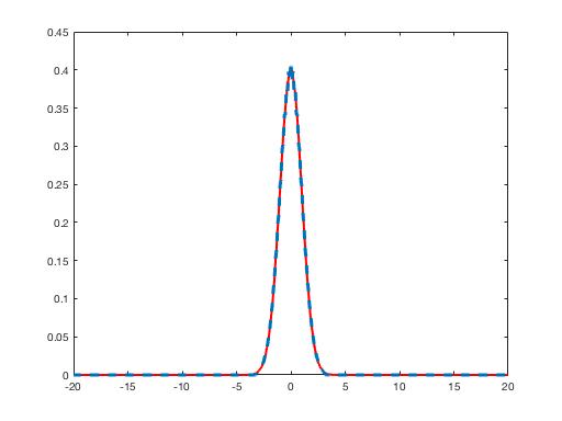
(a) Predicated, Time $t=1$.

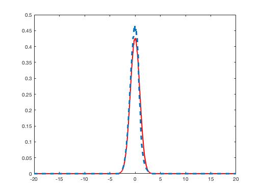
(b) Filtered, Time $t=1$.

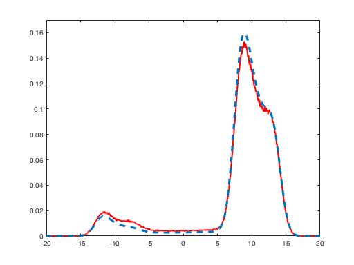
(c) Predicted, Time $t=5$.

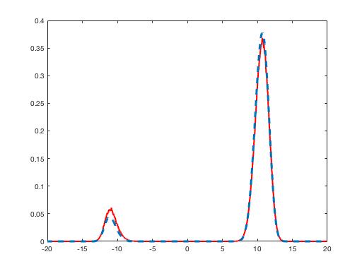
(d) Filtered, Time $t=5$.

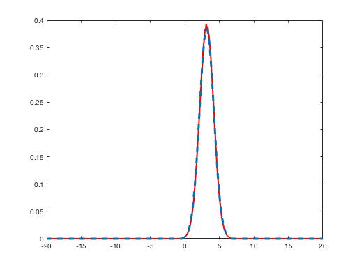
(e) Predicted, Time $t=50$.

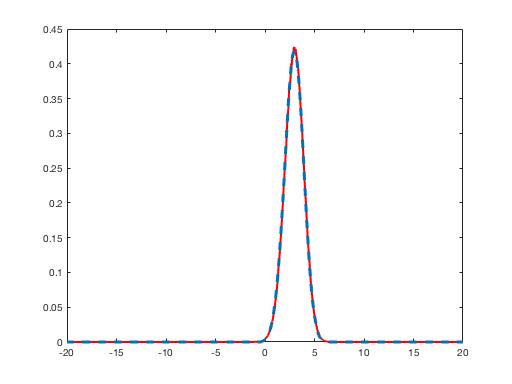
(f) Filtered, Time $t=50$.

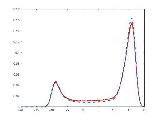
(g) Predicted, Time $t=80$.

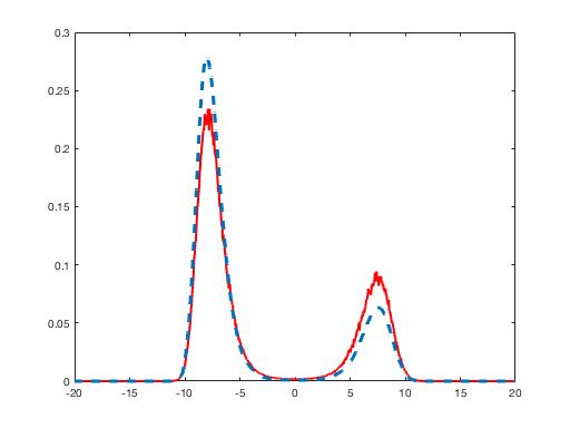
(h) Filtered, Time $t=80$.

Figure 7: The predicted and filtered state densities. In each case, the GMMF density (blue) is compared against the density from a SMC method (red).

6 CONCLUSIONS AND FUTURE WORKS

In this paper we present a novel square-root form Bayesian filtering algorithm for state-space models that can be described using a Gaussian mixture for both the process and measurement PDFs. The main attraction of restricting attention to this class of models is that the time and measurement update equations can be solved in closed form. This comes at the expense of exponential growth in computational load, which we combat by employing a Kullback–Leibler reduction method at each stage of the filter. The proposed algorithm is profiled on several examples including non-linear models that fall strictly outside the model class. Interestingly, this does not appear to pose a serious problem for the algorithm.

References

- [1] B. Ristic, S. Arulampalam, and N. Gordon, Beyond the Kalman Filter: Particle Filters for Tracking Applications. Boston, MA, USA: Artech house, 2004.
- [2] S. Thrun, W. Burgard, and D. Fox, Probabilistic Robotics. Intelligent robotics and autonomous agents, MIT Press, 2005.
- [3] T. Ardeshiri, U. Orguner, C. Lundquist, and T. B. Schön, “On mixture reduction for multiple target tracking,” in Information Fusion (FUSION), 2012 15th International Conference on, pp. 692–699, IEEE, 2012.
- [4] J. Yu, “A particle filter driven dynamic gaussian mixture model approach for complex process monitoring and fault diagnosis,” Journal of Process Control, vol. 22, no. 4, pp. 778–788, 2012.
- [5] T. B. Schön, A. Wills, and B. Ninness, “System identification of nonlinear state-space models,” Automatica, vol. 37, pp. 39–49, jan 2011.
- [6] R. E. Kalman, “A new approach to linear filtering and prediction problems,” Trans. ASME Series D: J. Basic Eng., vol. 82, pp. 35–45, 1960.
- [7] G. Smith, S. Schmidt, and L. McGee, “Application of statistical filter theory to the optimal estimation of position and velocity on board a circumlunar vehicle,” tech. rep., NASA,Tech. Rep. NASA TR-135,, 1962.
- [8] S. J. Julier, J. K. Uhlmann, and H. F. Durrant-Whyte, “A new approach for filtering nonlinear systems,” in American Control Conference, Proceedings of the 1995, vol. 3, pp. 1628–1632, IEEE, 1995.
- [9] N. J. Gordon, D. J. Salmond, and A. F. M. Smith, “A novel approach to nonlinear/non-Gaussian Bayesian state estimation,” in IEE Proceedings on Radar and Signal Processing, vol. 140, pp. 107–113, 1993.
- [10] A. Bacharoglou, “Approximation of probability distributions by convex mixtures of gaussian measures,” Proceedings of the American Mathematical Society, vol. 138, no. 7, pp. 2619–2628, 2010.
- [11] D. Alspach and H. Sorenson, “Nonlinear bayesian estimation using gaussian sum approximations,” IEEE transactions on automatic control, vol. 17, no. 4, pp. 439–448, 1972.
- [12] M. Simandl and J. Dunik, “Sigma point gaussian sum filter design using square root unscented filters,” IFAC Proceedings Volumes, vol. 38, no. 1, pp. 1000–1005, 2005.
- [13] J. H. Kotecha and P. M. Djuric, “Gaussian sum particle filtering,” IEEE Transactions on signal processing, vol. 51, no. 10, pp. 2602–2612, 2003.
- [14] D. Raihan and S. Chakravorty, “Particle gaussian mixture (pgm) filters,” in Information Fusion (FUSION), 2016 19th International Conference on, pp. 1369–1376, IEEE, 2016.
- [15] P. Fearnhead, “Particle filters for mixture models with an unknown number of components,” Statistics and Computing, vol. 14, no. 1, pp. 11–21, 2004.
- [16] D. Crouse, P. Willett, K. Pattipati, and L. Svensson, “A look at gaussian mixture reduction algorithms,” in in Proceedings of the 14th International Conference on Information Fusion (FUSION), 2011.
- [17] A. R. Runnalls, “Kullback-leibler approach to gaussian mixture reduction,” IEEE Transactions on Aerospace and Electronic Systems, vol. 43, no. 3, 2007.
- [18] W. B. Whitman, D. C. Coleman, and W. J. Wiebe, “Prokaryotes: the unseen majority,” Proceedings of the National Academy of Sciences, vol. 95, no. 12, pp. 6578–6583, 1998.
- [19] T. Kailath, A. H. Sayed, and B. Hassibi, Linear Estimation. Prentice Hall, 2000.
- [20] A. Doucet, S. J. Godsill, and C. Andrieu, “On sequential Monte Carlo sampling methods for Bayesian filtering,” Statistics and Computing, vol. 10, no. 3, pp. 197–208, 2000.
- [21] S. J. Godsill, A. Doucet, and M. West, “Monte Carlo smoothing for nonlinear time series,” Journal of the American Statistical Association, vol. 99, pp. 156–168, Mar. 2004.