Maximum Signal Minus Interference to Noise Ratio Multiuser Receive Beamforming

Abstract

Motivated by massive deployment of low data rate Internet of things (IoT) and ehealth devices with requirement for highly reliable communications, this paper proposes receive beamforming techniques for the uplink of a single-input multiple-output (SIMO) multiple access channel (MAC), based on a per-user probability of error metric and one-dimensional signalling. Although beamforming by directly minimizing probability of error (MPE) has potential advantages over classical beamforming methods such as zero-forcing and minimum mean square error beamforming, MPE beamforming results in a non-convex and a highly nonlinear optimization problem. In this paper, by adding a set of modulation-based constraints, the MPE beamforming problem is transformed into a convex programming problem. Then, a simplified version of the MPE beamforming is proposed which reduces the exponential number of constraints in the MPE beamforming problem. The simplified problem is also shown to be a convex programming problem. The complexity of the simplified problem is further reduced by minimizing a convex function which serves as an upper bound on the error probability. Minimization of this upper bound results in the introduction of a new metric, which is termed signal minus interference to noise ratio (SMINR). It is shown that maximizing SMINR leads to a closed-form expression for beamforming vectors as well as improved performance over existing beamforming methods.

I Introduction

In wireless communications, remarkable advantages such as diversity, spatial multiplexing gain, and higher throughput for single-user and multiuser systems are achieved by using multiple transmit and receive antennas [1, 2, 3, 4, 5]. In a system which exploits antenna arrays, space division multiple access (SDMA) techniques could be used to obtain spatial multiplexing gain and to significantly increase the achievable system throughput [6, 7, 8]. Linear and nonlinear beamforming techniques employed with an antenna array achieve spatial multiplexing by separating users’ signals transmitted simultaneously and on the same carrier frequency, provided that their channels are linearly independent [7, 9, 10]. Classically, beamforming weights can be determined by maximizing signal to noise ratio (SNR), nulling the interference, i.e., zero-forcing (ZF) co-channel interference, minimizing mean square error (MSE) between the desired signal and the array output, maximizing signal to interference and noise ratio (SINR), or minimizing the received signal variance while keeping the system response distortionless (MVDR) [11, 12, 13]. However, in digital communications systems, the error probability more closely reflects actual quality of service (QoS) [14, 15, 16, 17]. Therefore, beamforming weights ought to be set with the goal of directly minimizing the error probability.

Directly minimizing the error probability was considered in [18, 19] for designing equalizers to combat intersymbol interference (ISI). Later, this approach was adopted in a multiuser detection (MUD) scenario to estimate the received signals by minimizing the probability of error in a code division multiple access (CDMA) system [14, 20, 21]. Minimum probability of error (MPE) beamforming was studied in [22, 23, 10] by extending the ideas of MPE detection in CDMA systems and MPE equalization for ISI removal to the problem of spatial multiplexing and receive beamforming.

It has been shown in [24, 22] that MPE beamforming substantially outperforms ZF beamforming, minimum mean square error (MMSE) beamforming, and other classical receive beamforming methods. Nevertheless, the probability of error function in a multiuser system is highly nonlinear and suffers from the existence of numerous local minima [20, 24]. This issue has been resolved for the special case of MPE beamforming with binary phase shift keying (BPSK) by transforming the nonconvex nonlinear MPE beamforming problem to a convex optimization problem in [24]. Nevertheless, the high computational complexity of the problem in [24] is still an unresolved issue, besides its limitation to BPSK signalling.

In this paper, not only the idea of convex MPE beamforming is extended from BPSK to general one-dimensional (1D) signalling, but also the issue of high computational complexity is addressed. First, we calculate the error probability of each pulse amplitude modulated user in the uplink of a multiple access wireless system. Then, we formulate a beamforming problem by minimizing the error probability of each user. The minimum probability of error beamforming is then transformed to a convex optimization problems with a unique solution. Next, the exponential complexity of the problem is reduced by decreasing the number of constraints in the optimization. Subsequently, we further reduce the complexity of the problem by minimizing an upper bound on the error probability of each user. Finally, derived from the error probability, a new metric is presented, which we term signal minus interference to noise ratio (SMINR). Maximization of this metric results in a closed-form solution for the beamforming weights of each user. It will be seen that maximizing SMINR also results in improved performance compared to that of conventional ZF and MMSE beamforming.

The Internet of things (IoT) requires simultaneous deployment of a massive number of low data rate devices [25, 26]. Therefore, a motivation for considering one-dimensional signalling is the emergence of technologies such as IoT. Moreover, power efficient BPSK, a special case of one-dimensional modulation, is a commonly employed transmission mode in adaptive wireless systems such as IEEE 802.11a,n,ac, when SNR is low [27, 28].

The rest of this paper is organized as follows: Section II introduces the system model. In Section III, the exact error probability of each user in a vector multiple access channel is calculated for one-dimensional modulation. In Section IV, the MPE beamforming problem is transformed into a convex optimization problem. Section V reduces the complexity of convex MPE beamforming problem and introduces the SMINR criterion and maximum SMINR beamforming. Numerical results are presented in Section VI. Finally, conclusions are drawn in Section VII.

The following mathematical notation is used throughout the paper. Boldface upper case and lower case letters denote matrices and vectors, respectively. The superscripts $(\cdot)^{T}$, $(\cdot)^{H}$ denote the transpose and conjugate transpose, respectively. The eigenvector corresponding to the maximum eigenvalue is denoted by ${\bf v}_{\text{max}}$. $\|\cdot\|_{2}$ denotes the $\ell_{2}$-norm. $\Re\{\cdot\}$ and $\Im\{\cdot\}$ represent real and imaginary parts of complex numbers/matrices, respectively.

II System Model

We consider a multiple access system supporting $K$ power-limited users, where each user transmits a pulse amplitude modulated signal. It is assumed that users are in the far-field region of a linear antenna array with $N$ elements. It is further assumed that users transmit their signals on the same carrier frequency, $f_{c}$. Baseband pulse amplitude modulated signal of user $k$ is represented by

$$s_{k}(t;l_{k})=A_{k}(l_{k})g(t),\quad 1\leq k\leq K,$$ (1)

only over a real basis function, where $A_{k}(l_{k})$ takes on values from the set

$$\{(2l_{k}-1-L_{k})d|~{}1\leq l_{k}\leq L_{k}\}$$ (2)

with equal probability and $2d$ is the distance between adjacent signal constellation points. Therefore, in vector space form, the transmitted signal of user $k$ is represented by

$$s_{k}(l_{k})=\sqrt{E_{g}}A_{k}(l_{k}),\quad 1\leq k\leq K.$$ (3)

Assuming fading channels and additive noise, the $N$-dimensional received signal vector, ${\bf{r}}$ is represented by

$${\bf r}={\bf H}{\bf s}+{\bf z},$$ (4)

where ${\bf H}=[{\bf h}_{1},\cdots,{\bf h}_{K}]$ and ${\bf h}_{k}$ is the $N$-dimensional channel vector between transmitter $k$ and the $N$ receive antennas. The components of the ${\bf h}_{k}$s are assumed to follow an independent identically distributed (i.i.d.) circularly symmetric complex Gaussian (CSCG) distribution with zero mean and unit variance. This channel model is valid for narrowband (frequency non-selective) systems if the transmit and receive antennas are in non line-of-sight rich-scattering environments with sufficient antenna spacing [29, 30]. In (4), ${\bf s}=[{s}_{1},\ldots,{s}_{K}]^{T}$, where $s_{k}=s_{k}(l_{k})$ and the noise ${\bf z}$ is an $N$-dimensional vector, the elements of which are mutually independent identically distributed CSCG random variables with zero mean and variance $\sigma_{z}^{2}$.

Assuming linear processing at the receiver, the array output for user $k$ can be written as a function of the received filter of user $k$ as

$$y_{k} ={\bf w}_{k}{\bf r}={\bf w}_{k}{\bf H}{\bf s}+{\bf w}_{k}{\bf z}=\sum_{j=1}^{K}{\bf w}_{k}{\bf h}_{j}s_{j}+{\bf w}_{k}{\bf z}$$

$$={\bf w}_{k}{\bf h}_{k}s_{k}+{\bf w}_{k}{\bf H}_{\bar{k}}{\bf s}_{\bar{k}}+{\bf w}_{k}{\bf z}$$

$$={\bar{y}}_{k}+{z^{\prime}_{k}},\quad 1\leq k\leq K,$$ (5)

where ${\bf w}_{k}$ is the $1\times N$ complex-valued receive beamformer of user $k$, $z^{\prime}_{k}$ is a complex valued Gaussian noise with variance $\sigma_{z}^{2}{\bf w}_{k}{\bf w}_{k}^{H}$, ${\bf s}_{\bar{k}}=[s_{1},\cdots,s_{k-1},s_{k+1},\cdots,s_{K}]^{T}$, and ${\bf H}_{\bar{k}}=[{\bf h}_{1},\cdots,{\bf h}_{k-1},{\bf h}_{k+1},\cdots,{\bf h}_{K}]$.

III Error Probability

Since the information signal is one-dimensionally modulated only on a real basis function, without loss of generality, the decision is performed only over the real part of the output of the receive beamformer. For $1\leq k\leq K$, we consider the following decision rule for estimating the transmitted symbols of user $k$:

$${\hat{s}}_{k}$$

$$=\left\{\begin{array}[]{lr}s_{k}(1)&y_{k}^{R}\leq\Re\{{\bf w}_{k}{\bf h}_{k}s_{k}(1)+{\bf w}_{k}{\bf h}_{k}d\sqrt{E_{g}}\}\\[7.22743pt] s_{k}(l_{k})&\begin{array}[]{r}\Re\{{\bf w}_{k}{\bf h}_{k}s_{k}(l_{k})-{\bf w}_{k}{\bf h}_{k}d\sqrt{E_{g}}\}<y_{k}^{R}\\ \leq\Re\{{\bf w}_{k}{\bf h}_{k}s_{k}(l_{k})+{\bf w}_{k}{\bf h}_{k}d\sqrt{E_{g}}\};\\ 2\leq l_{k}\leq L_{k}-1\end{array}\\[18.06749pt] s_{k}(L_{k})&y_{k}^{R}>\Re\{{\bf w}_{k}{\bf h}_{k}s_{k}(L_{k})-{\bf w}_{k}{\bf h}_{k}d\sqrt{E_{g}}\}\end{array}\right.,$$ (12)

where the superscript ^R denotes the real part, i.e., $x^{R}={\Re}\{x\}$.

The error probability of user $k$ is expressed as

$$P_{e_{k}}\!=\!\sum_{l_{k}=1}^{L_{k}}\!P(l_{k})P_{e_{k}}(l_{k})\!=\!\frac{1}{L_{k}}\!\sum_{l_{k}=1}^{L_{k}}\!P({\hat{s}}_{k}\!\neq\!s_{k}(l_{k})|s_{k}\!=\!s_{k}(l_{k}))$$

$$=\!\frac{1}{L_{k}}\!\left[\!P(y_{k}^{R}\!>\!\Re\{{\bf w}_{k}{\bf h}_{k}s_{k}(1)\!+\!{\bf w}_{k}{\bf h}_{k}d\sqrt{E_{g}}\}|s_{k}\!=\!s_{k}(1))\right.$$

$$\!+\!\!\sum_{l_{k}\!=\!2}^{L_{k}\!-\!1}\!\!P(|y_{k}^{R}\!\!-\!\Re\{{\bf w}_{k}{\bf h}_{k}s_{k}(l_{k}\!)\}|\!\!>\!\!\Re\{{\bf w}_{k}{\bf h}_{k}d\sqrt{\!E_{g}}\}\!|s_{k}\!\!=\!\!s_{k}(l_{k}))$$

$$+\!\left.P(y_{k}^{R}\!\leq\!\Re\{{\bf w}_{k}{\bf h}_{k}s_{k}(L_{k})\!-\!{\bf w}_{k}{\bf h}_{k}d\sqrt{E_{g}}\}|s_{k}\!=\!s_{k}(L_{k}))\!\right]$$ (13)

where $P(\cdot)$ is the probability of an event and $P(l_{k})=P(s_{k}=s_{k}(l_{k}))=\frac{1}{L_{k}}$, i.e., the transmitted PAM signal $s_{k}$ takes its values from the set (2) with equal probability. The error probability of user $k$, given $s_{k}(l_{k})$ is transmitted, is denoted by $P_{e_{k}}(l_{k})$. It should be remarked that assuming uniform (as we did) rather than Gaussian distribution over signal sets, although more practical, causes an asymptotic loss in throughput which could be compensated to some extent by using constellation shaping techniques [28].

To calculate the error probability (III), first we need to find the probability density function (pdf) of $y_{k}^{R}$ conditioned on $s_{k}$, namely, $p(y_{k}^{R}|s_{k})$. Let us denote the number of possible symbol sequences of all $K$ users in one transmission by $N_{b}=\prod_{k=1}^{K}L_{k}$, i.e., there could be $N_{b}$ different possible sets of $K$-tuple symbols ${\bf s}$ for $K$ users. Moreover, let $N_{p_{k}}=\prod_{\begin{subarray}{c}j=1\\ j\neq k\end{subarray}}^{K}L_{j}$ denote the number of possible vector of symbols for transmission if the transmitted symbol of user $k$ is already known, i.e., there could be $N_{p_{k}}$ different possible sets of $K-1$-tuple symbols ${\bf s}_{\bar{k}}(b),~{}1\leq b\leq N_{p_{k}},$ for $K-1$ users. Using equal probability for transmission of PAM constellation points, and Gaussian output noise $\Re\{z^{\prime}_{k}\}$, we have

$$p(y_{k}^{R}|s_{k}=s_{k}(l_{k}))=\frac{1}{N_{p_{k}}}\sum_{\forall{\bf s}_{\bar{k}}}p(y_{k}^{R}|s_{k}=s_{k}(l_{k}),{\bf s}_{\bar{k}})$$

$$=\frac{1}{N_{p_{k}}}\sum_{b=1}^{N_{p_{k}}}p(y_{k}^{R}|s_{k}=s_{k}(l_{k}),{\bf s}_{\bar{k}}={\bf s}_{\bar{k}}(b))$$

$$=\frac{1}{N_{p_{k}}}\sum_{b=1}^{N_{p_{k}}}\frac{1}{\sqrt{\pi\sigma_{z}^{2}{\bf w}_{k}{\bf w}_{k}^{H}}}\exp{-\frac{(y_{k}^{R}-{\bar{y}}_{k}^{R}(l_{k},b))^{2}}{\sigma_{z}^{2}\|{\bf w}_{k}\|_{2}^{2}}},$$ (14)

where in the first equality the total probability theorem is used to condition the conditional output probability of user $k$ over all $N_{p_{k}}$ possible symbol assignment of the transmitted symbols ${\bf s}_{\bar{k}}$. Also ${\bar{y}}_{k}^{R}(l_{k},b)={\Re}\{{\bar{y}}_{k}\}$ when $s_{k}=s_{k}(l_{k})$ and ${\bf s}_{\bar{k}}={\bf s}_{\bar{k}}(b)$, i.e.,

$${\bar{y}}_{k}^{R}(l_{k},b)=\Re\{{\bf w}_{k}{\bf h}_{k}s_{k}(l_{k})+{\bf w}_{k}{\bf H}_{\bar{k}}{\bf s}_{\bar{k}}(b)\},$$

$$\quad 1\leq l_{k}\leq L_{k},~{}1\leq b\leq N_{p_{k}}.$$ (15)

Having the conditional pdf of $y_{k}^{R}$ as in (III), each of the three terms in the last equality of (III) can be calculated as follows:

$$P\left(y_{k}^{R}>\Re\{{\bf w}_{k}{\bf h}_{k}s_{k}(1)+{\bf w}_{k}{\bf h}_{k}d\sqrt{E_{g}}\}|s_{k}=s_{k}(1)\right)$$

$$=\int_{\Re\{{\bf w}_{k}{\bf h}_{k}s_{k}(1)+{\bf w}_{k}{\bf h}_{k}d\sqrt{E_{g}}\}}^{\infty}\frac{1}{N_{p_{k}}}\sum_{b=1}^{N_{p_{k}}}\frac{1}{\sqrt{\pi\sigma_{z}^{2}{\bf w}_{k}{\bf w}_{k}^{H}}}$$

$$\times\exp{-\frac{(y_{k}^{R}-{\bar{y}}_{k}^{R}(1,b))^{2}}{\sigma_{z}^{2}\|{\bf w}_{k}\|_{2}^{2}}}dy_{k}^{R}$$

$$=\frac{1}{N_{p_{k}}}\sum_{b=1}^{N_{p_{k}}}Q\left(\frac{\Re\{{\bf w}_{k}{\bf h}_{k}d\sqrt{E_{g}}-{\bf w}_{k}{\bf H}_{\bar{k}}{\bf s}_{\bar{k}}(b)\}}{\frac{\sigma_{z}}{\sqrt{2}}\|{\bf w}_{k}\|_{2}}\right),$$

$$1\leq k\leq K,$$ (16)

where the $Q$-function is defined as $Q(x)=\frac{1}{\sqrt{2\pi}}\int_{x}^{\infty}{e^{-\frac{u^{2}}{2}}du}$, and we used the property

$$\frac{1}{\sqrt{2\pi\sigma^{2}}}\int_{x}^{\infty}\exp\left(-\frac{(u-\bar{u})^{2}}{2\sigma^{2}}\right)\,du=Q(\frac{x-\bar{u}}{\sigma}).$$ (17)

The third part of the last equality in (III) is calculated as

$$P\left(y_{k}^{R}\leq\Re\{{\bf w}_{k}{\bf h}_{k}s_{k}(L_{k})-{\bf w}_{k}{\bf h}_{k}d\sqrt{E_{g}}\}|s_{k}=s_{k}(L_{k})\right)$$

$$=\int_{-\infty}^{\Re\{{\bf w}_{k}{\bf h}_{k}s_{k}(L_{k})-{\bf w}_{k}{\bf h}_{k}d\sqrt{E_{g}}\}}\frac{1}{N_{p_{k}}}\sum_{b=1}^{N_{p_{k}}}$$

$$\frac{1}{\sqrt{\pi\sigma_{z}^{2}{\bf w}_{k}{\bf w}_{k}^{H}}}\exp{-\frac{(y_{k}^{R}-{\bar{y}}_{k}^{R}(L_{k},b))^{2}}{\sigma_{z}^{2}\|{\bf w}_{k}\|_{2}^{2}}}dy_{k}^{R}$$

$$=\frac{1}{N_{p_{k}}}\sum_{b=1}^{N_{p_{k}}}Q\left(\frac{\Re\{{\bf w}_{k}{\bf h}_{k}d\sqrt{E_{g}}+{\bf w}_{k}{\bf H}_{\bar{k}}{\bf s}_{\bar{k}}(b)\}}{\frac{\sigma_{z}}{\sqrt{2}}\|{\bf w}_{k}\|_{2}}\right),$$

$$1\leq k\leq K,$$ (18)

where we used the property

$$\frac{1}{\sqrt{2\pi\sigma^{2}}}\int_{-\infty}^{x}\exp\left(-\frac{(u-\bar{u})^{2}}{2\sigma^{2}}\right)\,du=Q(\frac{\bar{u}-x}{\sigma}).$$ (19)

The second part of the last equality in (III) is calculated as

$$P\left(|y_{k}^{R}-\Re\{{\bf w}_{k}{\bf h}_{k}s_{k}(l_{k})\}|\!>\!\Re\{{\bf w}_{k}{\bf h}_{k}d\sqrt{E_{g}}\}|s_{k}\!=\!s_{k}(l_{k})\right)$$

$$\!=\!P\left(y_{k}^{R}\!-\!\Re\{{\bf w}_{k}{\bf h}_{k}s_{k}(l_{k})\}\!>\!\Re\{{\bf w}_{k}{\bf h}_{k}d\sqrt{E_{g}}\}|s_{k}\!=\!s_{k}(l_{k})\right)$$

$$\!+\!P\!\left(\!y_{k}^{R}\!-\!\Re\{\!{\bf w}_{k}{\bf h}_{k}s_{k}(l_{k})\}\!<\!\!-\Re\{{\bf w}_{k}{\bf h}_{k}d\sqrt{E_{g}}\}|s_{k}\!=\!s_{k}(l_{k})\right)$$

$$\!=\!\frac{1}{N_{p_{k}}}\sum_{b=1}^{N_{p_{k}}}\left[Q(\frac{\Re\{{\bf w}_{k}{\bf h}_{k}d\sqrt{E_{g}}-{\bf w}_{k}{\bf H}_{\bar{k}}{\bf s}_{\bar{k}}(b)\}}{\frac{\sigma_{z}}{\sqrt{2}}\|{\bf w}_{k}\|_{2}})\right.$$

$$\!+\left.Q(\frac{\Re\{{\bf w}_{k}{\bf h}_{k}d\sqrt{E_{g}}\!+\!{\bf w}_{k}{\bf H}_{\bar{k}}{\bf s}_{\bar{k}}(b)\}}{\frac{\sigma_{z}}{\sqrt{2}}\|{\bf w}_{k}\|_{2}})\right]\!,$$

$$2\leq l_{k}\leq L_{k}-2,\quad 1\leq k\leq K,$$ (20)

where (17) and (19) are used. Finally, using (III), (III), (III), and (III) yields the error probability of user $k$:

$$P_{e_{k}}=\frac{L_{k}-1}{N_{b}}\sum_{b=1}^{N_{p_{k}}}$$

$$\left[Q\left(\frac{\Re\{{\bf w}_{k}{\bf h}_{k}d\sqrt{E_{g}}-{\bf w}_{k}{\bf H}_{\bar{k}}{\bf s}_{\bar{k}}(b)\}}{\frac{\sigma_{z}}{\sqrt{2}}\|{\bf w}_{k}\|_{2}}\right)\right.$$

$$+\left.Q\left(\frac{\Re\{{\bf w}_{k}{\bf h}_{k}d\sqrt{E_{g}}+{\bf w}_{k}{\bf H}_{\bar{k}}{\bf s}_{\bar{k}}(b)\}}{\frac{\sigma_{z}}{\sqrt{2}}\|{\bf w}_{k}\|_{2}}\right)\right].$$ (21)

To proceed further, the following property is required:

Property 1

For a given user

$$\sum_{b=1}^{N_{p_{k}}}Q\left(\frac{\Re\{{\bf w}_{k}{\bf h}_{k}d\sqrt{E_{g}}-{\bf w}_{k}{\bf H}_{\bar{k}}{\bf s}_{\bar{k}}(b)\}}{\frac{\sigma_{z}}{\sqrt{2}}\|{\bf w}_{k}\|_{2}}\right)$$

$$=\sum_{b=1}^{N_{p_{k}}}Q\left(\frac{\Re\{{\bf w}_{k}{\bf h}_{k}d\sqrt{E_{g}}+{\bf w}_{k}{\bf H}_{\bar{k}}{\bf s}_{\bar{k}}(b)\}}{\frac{\sigma_{z}}{\sqrt{2}}\|{\bf w}_{k}\|_{2}}\right).$$ (22)

Proof:

The pulse amplitude modulated signal constellation of each user is symmetric about zero. Therefore, for every given $b=b_{1}$ there exists a $b=\bar{b}_{1}$ such that ${\bf s}_{\bar{k}}(b_{1})=-{\bf s}_{\bar{k}}(\bar{b}_{1})$. Therefore,

$$Q(\frac{\Re\{{\bf w}_{k}{\bf h}_{k}d\sqrt{E_{g}}-{\bf w}_{k}{\bf H}_{\bar{k}}{\bf s}_{\bar{k}}(b_{1})\}}{\frac{\sigma_{z}}{\sqrt{2}}\|{\bf w}_{k}\|_{2}})$$

$$=Q(\frac{\Re\{{\bf w}_{k}{\bf h}_{k}d\sqrt{E_{g}}+{\bf w}_{k}{\bf H}_{\bar{k}}{\bf s}_{\bar{k}}(\bar{b}_{1})\}}{\frac{\sigma_{z}}{\sqrt{2}}\|{\bf w}_{k}\|_{2}}).$$ (23)

Hence,

$$\sum_{b=1}^{N_{p_{k}}}Q\left(\frac{\Re\{{\bf w}_{k}{\bf h}_{k}d\sqrt{E_{g}}-{\bf w}_{k}{\bf H}_{\bar{k}}{\bf s}_{\bar{k}}(b)\}}{\frac{\sigma_{z}}{\sqrt{2}}\|{\bf w}_{k}\|_{2}}\right)$$

$$=\sum_{\bar{b}=1}^{N_{p_{k}}}Q\left(\frac{\Re\{{\bf w}_{k}{\bf h}_{k}d\sqrt{E_{g}}+{\bf w}_{k}{\bf H}_{\bar{k}}{\bf s}_{\bar{k}}(\bar{b})\}}{\frac{\sigma_{z}}{\sqrt{2}}\|{\bf w}_{k}\|_{2}}\right)$$

$$=\sum_{b=1}^{N_{p_{k}}}Q\left(\frac{\Re\{{\bf w}_{k}{\bf h}_{k}d\sqrt{E_{g}}+{\bf w}_{k}{\bf H}_{\bar{k}}{\bf s}_{\bar{k}}(b)\}}{\frac{\sigma_{z}}{\sqrt{2}}\|{\bf w}_{k}\|_{2}}\right).$$ (24)

∎

Using Property 1, the error probability of user $k$ (III) can be expressed as

$$P_{e_{k}}= \frac{2(L_{k}-1)}{L_{k}N_{p}}\sum_{b=1}^{N_{p_{k}}}Q\left(\frac{\Re\{{\bf w}_{k}{\bf h}_{k}d\sqrt{E_{g}}+{\bf w}_{k}{\bf H}_{\bar{k}}{\bf s}_{\bar{k}}(b)\}}{\frac{\sigma_{z}}{\sqrt{2}}\|{\bf w}_{k}\|_{2}}\right)$$

$$= \frac{2(L_{k}-1)}{L_{k}N_{p}}\sum_{b=1}^{N_{p_{k}}}Q\left(\frac{\Re\{{\bf w}_{k}{\bf h}_{k}d\sqrt{E_{g}}-{\bf w}_{k}{\bf H}_{\bar{k}}{\bf s}_{\bar{k}}(b)\}}{\frac{\sigma_{z}}{\sqrt{2}}\|{\bf w}_{k}\|_{2}}\right).$$ (25)

III-A Minimum Probability of Error (MPE) Receive Beamforming

Knowing each user’s modulation type, its receive beamforming weights can be calculated by minimizing its probability of error. Therefore, the minimum probability of error (MPE) beamforming weights are the solutions to the following optimization problem:

$${\bf{w}}_{k_{\text{MPE}}}=\operatorname*{argmin}_{{\bf w}_{k}}P_{e_{k}},\quad 1\leq k\leq K,$$ (26)

where $P_{e_{k}}$ is the error probability of user $k$ defined in (III). As it can be seen from (26) and (III), the objective function of MPE beamforming problem, i.e., the error probability of user $k$ in the uplink of a multiuser system is a non-convex and nonlinear function of beamforming vector ${\bf w}_{k}$. While in general the non-convex and nonlinear optimization problem (26) can be solved by using exhaustive (brute force) search to achieve a global minimum, its computational complexity is prohibitive [31]. On the other hand, gradient-based optimization algorithms such as BFGS [31] can at best guarantee local stationary points. In our simulations, it was observed that if the initial point for the gradient-based optimization algorithm is not chosen appropriately, the algorithm converges to a drastically poor solution. Therefore, a more practical approach is necessary to solve (26).

IV Convex Optimization Based MPE Receive Beamforming

In this section, similar to [20] the MPE receive beamforming problem is transformed into a convex optimization problem with a unique solution which can be obtained by conventional convex programming algorithms such as interior point methods [32].

First, it should be remarked that ideally the error probability of all users in a MAC channel should approach zero when the transmit power of users approach infinity. To this end, we define the error floor as follows:

Definition 1

If the transmit powers of all users approach infinity and yet the average error probability cannot approach zero, the value of the tight lower bound on the average of the error probability is called the error floor.

Proposition 1

For the users not to have an error floor, it is necessary for ${\bf w}_{k},~{}1\leq k\leq K$ to comply with the following constraints:

$${\Re\{{\bf w}_{k}{\bf h}_{k}d\sqrt{E_{g}}-{\bf w}_{k}{\bf H}_{\bar{k}}{\bf s}_{\bar{k}}(b)\}}\geq 0,\quad 1\leq b\leq N_{p_{k}}.$$ (27)

Proof:

See Appendix A. ∎

Property 2

The error probability in (III) is invariant to the scaling of ${\bf w}_{k}$ by a positive constant.

Proof:

See Appendix B. ∎

From Proposition 1 and Property 2, it becomes clear that when no error floor exists, without loss of generality, the constraints $\|{\bf w}_{k}\|=1$ and (27) can be added to the optimization problem (26). Therefore, the MPE beamforming problem could be rewritten as follows.

$${\bf{w}}_{k_{\text{MPE}}}=\operatorname*{argmin}_{{\bf w}_{k}}P_{e_{k}}$$ (28a)

$$\text{subject to}\quad\|{\bf w}_{k}\|_{2}=1$$ (28b)

$$\quad\quad\quad\quad\quad\Re\{{\bf w}_{k}{\bf h}_{k}d\sqrt{E_{g}}-{\bf w}_{k}{\bf H}_{\bar{k}}{\bf s}_{\bar{k}}(b)\}\!\geq\!0,1\!\leq\!b\!\leq\!N_{p_{k}}.$$ (28c)

To solve the optimization problem (28), we have

Theorem 1

If the constraints (28b) and (28c) in the minimization problem (28) are satisfied, any local minimizer of error probability function $P_{e_{k}}$ (III), i.e., the objective function of the optimization problem (28), is also a global minimizer. Moreover, the global minimizer is unique.

Proof:

See Appendix C. ∎

Although Theorem 1 shows that the constrained MPE problem (28) has a unique global minimizer, (28) is not in the form of a standard convex programming problem. However, the constrained optimization problem (28) can be rewritten as follows:

$$\min_{{\bf w}_{k}}\frac{2(L_{k}-1)}{N_{b}}\sum_{b=1}^{N_{p_{k}}}Q\left(\frac{\Re\{{\bf w}_{k}{\bf h}_{k}d\sqrt{E_{g}}-{\bf w}_{k}{\bf H}_{\bar{k}}{\bf s}_{\bar{k}}(b)\}}{\frac{\sigma_{z}}{\sqrt{2}}}\right)$$ (29a)

$$\text{subject to}\quad\|{\bf w}_{k}\|_{2}=1,$$ (29b)

$$\quad\quad\quad\quad\quad\Re\{{\bf w}_{k}{\bf h}_{k}d\sqrt{E_{g}}-{\bf w}_{k}{\bf H}_{\bar{k}}{\bf s}_{\bar{k}}(b)\}\!\geq\!0,1\!\leq\!b\!\leq\!N_{p_{k}},$$ (29c)

which is the result of considering the equality constraint (28b) in the denominator of the $Q$-functions in (III). However, the constrained problem (29) is not a convex problem either, since the feasible region is not a convex set, which is due to the fact that (29b) is not a convex set. However, by transforming (29b) to

$$\|{\bf w}_{k}\|_{2}\leq 1,$$ (30)

the feasible region and therefore the optimization problem will become convex. Furthermore, the constraint set defined by (30) is an active set [31]. In other words, the minimizer always satisfies the constraint $\|{\bf w}_{k}\|_{2}=1$, because for $\|{\bf w}_{k}\|_{2}<1$, there always exists a ${\bf\hat{w}}_{k}=\frac{{\bf w}_{k}}{\|{\bf w}_{k}\|_{2}}$ for which $P_{e_{k}}({\bf\hat{w}}_{k})<P_{e_{k}}({\bf w}_{k})$. Therefore, the MPE receive beamforming problem can be cast into the following convex optimization problem with a unique global minimizer:

$$\min_{{\bf w}_{k}}\frac{2(L_{k}-1)}{N_{b}}\sum_{b=1}^{N_{p_{k}}}Q\left(\frac{\Re\{{\bf w}_{k}{\bf h}_{k}d\sqrt{E_{g}}-{\bf w}_{k}{\bf H}_{\bar{k}}{\bf s}_{\bar{k}}(b)\}}{\frac{\sigma_{z}}{\sqrt{2}}}\right)$$ (31a)

$$\text{subject to}\quad\|{\bf w}_{k}\|_{2}\leq 1$$ (31b)

$$\quad\quad\quad\quad\quad\Re\{{\bf w}_{k}{\bf h}_{k}d\sqrt{E_{g}}-{\bf w}_{k}{\bf H}_{\bar{k}}{\bf s}_{\bar{k}}(b)\}\!\geq\!0,1\!\leq\!b\!\leq\!N_{p_{k}}.$$ (31c)

Problem (31) can then be solved by conventional convex programming methods. For example by using the interior point methods, the complexity would be of polynomial order with respect to $N$ [31].

It is worth noting that the convex constrained problem (31) only has a solution when the set of constraints is feasible. If users in the original MPE beamforming problem (26) suffer from the existence of the error floor, it means that at least one of the constraints defined in (31c) do not hold for one of the users. Therefore, the set of constraints defined by (31b) and (31c) is empty for this user. In other words, the constrained problem does not have any solution for this user. It should be mentioned that if such an instance occurs, i.e., when users suffer from the existence of the error floor, it is inherently impossible for at least one of the users to be met by an acceptable quality of service using linear beamforming methods. This means that the received signals of such a user are not linearly separable using linear beamforming methods.

V Reduced-Complexity Convex MPE Beamforming

Although (31) is a convex optimization problem with low complexity in the number of receive antennas $N$, the number of constraints in (31c) and the number of summations in (31a) are of the order of $N_{p_{k}}=\prod_{\begin{subarray}{c}j=1\\ j\neq k\end{subarray}}^{K}L_{j}$, i.e., exponential in the number of users $K$ and polynomial in the modulation order $L$.

Proposition 2

A necessary and sufficient condition for all $N_{p_{k}}$ constraints of (31c) to hold is

$$\Re\{{\bf w}_{k}{\bf h}_{k}d\sqrt{E_{g}}\}-\sum_{\begin{subarray}{c}j=1\\ j\neq k\end{subarray}}^{K}|\Re\{{\bf w}_{k}{\bf h}_{j}s_{j}(L_{j})\}|\geq 0.$$ (32)

Proof:

See Appendix D. ∎

Replacing all $N_{p_{k}}$ constraints of (31c) with (32), the MPE receive beamforming problem (31) is equivalently converted to

$$\min_{{\bf w}_{k}}\frac{2(L_{k}-1)}{N_{b}}\sum_{b=1}^{N_{p_{k}}}Q\left(\frac{\Re\{{\bf w}_{k}{\bf h}_{k}d\sqrt{E_{g}}-{\bf w}_{k}{\bf H}_{\bar{k}}{\bf s}_{\bar{k}}(b)\}}{\frac{\sigma_{z}}{\sqrt{2}}}\right)$$ (33a)

$$\text{subject to}\quad\|{\bf w}_{k}\|_{2}\leq 1$$ (33b)

$$\quad\quad\quad\quad\quad~{}\Re\{{\bf w}_{k}{\bf h}_{k}d\sqrt{E_{g}}\}-\sum_{\begin{subarray}{c}j=1\\ j\neq k\end{subarray}}^{K}|\Re\{{\bf w}_{k}{\bf h}_{j}s_{j}(L_{j})\}|\geq 0,$$ (33c)

with reduced complexity.

Claim 1

Constraint set (33c) is a convex set.

Proof:

See Appendix E. ∎

Based on Claim 1 and the discussion in Section IV, it can be inferred that the reduced MPE beamforming problem (33) is a convex problem which can be solved using conventional convex programming methods [32].

V-A Maximum Signal Minus Interference to Noise Ratio (SMINR) Beamforming - Amplitude Version

To further reduce the complexity of (33), we replace the summation of $N_{p_{k}}$ terms in objective function (33a) by a single term which serves as an upper bound on the objective function.

Claim 2

The following expression is an upper bound on the error probability of user $k$ and therefore on the objective function (33a):

$$\tilde{P}_{e_{k}}^{\text{Up}}=\frac{2(L_{k}-1)}{L_{k}}$$

$$\times\!Q\left(\frac{\Re\{{\bf w}_{k}{\bf h}_{k}d\sqrt{E_{g}}\}-\sum_{\begin{subarray}{c}j=1\\ j\neq k\end{subarray}}^{K}|\Re\{{\bf w}_{k}{\bf h}_{j}s_{j}(L_{j})\}|}{\frac{\sigma_{z}}{\sqrt{2}}}\right)\!.$$ (34)

Proof:

Considering that the $Q$-function is decreasing for nonnegative arguments, and using (D) in Appendix D, it can be easily shown that (2) is an upper bound on the error probability of user $k$ and also an upper bound on the objective function (33a). ∎

Using (2), the beamforming problem is formulated by minimizing the upper bound on the error probability of each user:

$${\bf{w}}_{k_{\text{SMINR\_Amp}}}=\operatorname*{argmin}_{{\bf w}_{k}}\tilde{P}_{e_{k}}^{\text{Up}}$$ (35a)

$$\text{subject to}\quad\|{\bf w}_{k}\|_{2}\leq 1$$ (35b)

$$\quad\quad\quad\quad\quad~{}\Re\{{\bf w}_{k}{\bf h}_{k}d\sqrt{E_{g}}\}-\sum_{\begin{subarray}{c}j=1\\ j\neq k\end{subarray}}^{K}|\Re\{{\bf w}_{k}{\bf h}_{j}s_{j}(L_{j})\}|\geq 0.$$ (35c)

Since the argument of the $Q$-function in (2) is constrained to be nonnegative by (35c), and the $Q$-function is a decreasing function for nonnegative arguments, problem (35) is equivalent to

$${\bf w}_{k_{\text{SMINR\_Amp}}}=\operatorname*{argmax}_{{\bf w}_{k}}\text{ SMINR}_{\text{Amp}}$$ (36a)

$$\text{subject to}\quad\|{\bf w}_{k}\|_{2}\leq 1$$ (36b)

$$\quad\quad\quad\quad\quad~{}\Re\{{\bf w}_{k}{\bf h}_{k}d\sqrt{E_{g}}\}-\sum_{\begin{subarray}{c}j=1\\ j\neq k\end{subarray}}^{K}|\Re\{{\bf w}_{k}{\bf h}_{j}s_{j}(L_{j})\}|\geq 0,$$ (36c)

where

$$\text{SMINR}_{\text{Amp}}=\frac{\Re\{{\bf w}_{k}{\bf h}_{k}d\sqrt{E_{g}}\}-\sum_{\begin{subarray}{c}j=1\\ j\neq k\end{subarray}}^{K}|\Re\{{\bf w}_{k}{\bf h}_{j}s_{j}(L_{j})\}|}{\frac{\sigma_{z}}{\sqrt{2}}}.$$ (37)

The objective function of (36), i.e., (37) can be interpreted as the ratio of half the distance between two received signal constellation points minus the maximum amplitude of the interference from all other users relative to the noise standard deviation (square root of noise variance). We name this objective function signal minus interference to noise ratio (SMINR), amplitude-based version. Maximum SMINR beamforming-amplitude version (SMINR-Amp) (36) is a low-complexity convex optimization problem since the constraints (36c) and (36b) are convex sets as discussed in Claim 1 and the discussion in Section IV, respectively; also it can easily be shown that the objective function of (36) is a concave function by using the definition of convex and concave functions [32].

V-B Heuristic Maximum SMINR Beamforming

Although (36) is a low-complexity convex optimization problem, it still needs to be solved using numerical optimization methods. We next aim to formulate a similar problem to (36) that can be dealt with analytically to obtain a closed-form solution. To this end, we define a power-based version of SMINR as follows:

$$\text{SMINR}\triangleq\frac{(\Re\{{\bf w}_{k}{\bf h}_{k}d\sqrt{E_{g}}\})^{2}-\sum_{\begin{subarray}{c}j=1\\ j\neq k\end{subarray}}^{K}(\Re\{{\bf w}_{k}{\bf h}_{j}s_{j}(L_{j})\})^{2}}{\frac{\sigma_{z}^{2}}{2}}.$$ (38)

The following optimization problem is then introduced:

$${\bf w}_{k_{\text{SMINR}}}=\operatorname*{argmax}_{{\bf w}_{k}}\text{ SMINR}$$ (39a)

$$\text{subject to}\quad\|{\bf w}_{k}\|_{2}=1.$$ (39b)

Power-based SMINR (38), which for simplicity is termed SMINR henceforward, is differentiable with respect to ${\bf w}_{k}$ and method of Lagrange multipliers can be adopted to solve the corresponding optimization problem. Writing the Lagrangian and using Wirtinger calculus [33, 34, 35] to set the gradient of the Lagrangian with respect to ${\bf w}_{k}$ to zero, the following equation is obtained:

$$d^{2}E_{g}\Re\{{\bf w}_{k}{\bf h}_{k}\}{\bf h}_{k}^{T}\!-\!\sum_{\begin{subarray}{c}j=1\\ j\neq k\end{subarray}}^{K}s_{j}^{2}(L_{j})\Re\{{\bf w}_{k}{\bf h}_{j}\}{\bf h}_{j}^{T}\!+\!\mu\frac{\sigma_{z}^{2}}{2}{\bf w}_{k}^{*}\!=\!{\bf 0},$$ (40)

where $\mu$ is the Lagrange multiplier. Unfortunately, as can be seen from (40), ${\bf w}_{k}$ and ${\bf w}_{k}^{*}$ are coupled in a way that a closed-form solution cannot be obtained. Since the objective here was to find a closed-form solution for beamforming vectors, pursuing this approach is not of interest.

To tackle the coupling issue, the following transformations are employed for $1\leq k\leq K$:

$${\bf w}_{k}\in\mathbb{C}^{1\times N}\xrightarrow{\mathcal{T}_{1}}{\bf\bar{w}}_{k}=\left[\begin{array}[]{cc}\Re\{{\bf w}_{k}\}&\Im\{{\bf w}_{k}\}\end{array}\right]\in\mathbb{R}^{1\times 2N},$$ (42)

$${\bf h}_{k}\in\mathbb{C}^{N\times 1}\xrightarrow{\mathcal{T}_{2}}{\bf\tilde{h}}_{k}=\left[\begin{array}[]{c}\Re\{{\bf h}_{k}\}\\ -\Im\{{\bf h}_{k}\}\end{array}\right]\in\mathbb{R}^{2N\times 1}.$$ (45)

Using (42), maximum SMINR receive beamforming (39) is reformulated as

$${\bf\bar{w}}_{k_{\text{SMINR}}}=\operatorname*{argmax}_{{\bf\bar{w}}_{k}}\frac{({\bf\bar{w}}_{k}{\bf\tilde{h}}_{k}d\sqrt{E_{g}})^{2}-\sum_{\begin{subarray}{c}j=1\\ j\neq k\end{subarray}}^{K}({\bf\bar{w}}_{k}{\bf\tilde{h}}_{j}s_{j}(L_{j}))^{2}}{\frac{\sigma_{z}^{2}}{2}}$$ (46a)

$$\text{subject to}\quad\|{\bf\bar{w}}_{k}\|_{2}^{2}=1.$$ (46b)

Either by using Lagrange multipliers method or by rewriting (46) as the Rayleigh quotient problem

$$\max_{{\bf\bar{w}}_{k}}\frac{{\bf\bar{w}}_{k}\left(d^{2}E_{g}{\bf\tilde{h}}_{k}{\bf\tilde{h}}_{k}^{T}-\sum_{\begin{subarray}{c}j=1\\ j\neq k\end{subarray}}^{K}s_{j}^{2}(L_{j}){\bf\tilde{h}}_{j}{\bf\tilde{h}}_{j}^{T}\right){\bf\bar{w}}_{k}^{T}}{\frac{\sigma_{z}^{2}}{2}{\bf\bar{w}}_{k}{\bf\bar{w}}_{k}^{T}},$$ (47)

the solution is given by

$${\bf\bar{w}}_{k_{\text{SMINR}}}={\bf v}^{T}_{\text{max}}\left(d^{2}E_{g}{\bf\tilde{h}}_{k}{\bf\tilde{h}}_{k}^{T}-\sum_{\begin{subarray}{c}j=1\\ j\neq k\end{subarray}}^{K}s_{j}^{2}(L_{j}){\bf\tilde{h}}_{j}{\bf\tilde{h}}_{j}^{T}\right),$$ (48)

i.e., the normalized eigenvector corresponding to the maximum eigenvalue of $d^{2}E_{g}{\bf\tilde{h}}_{k}\allowbreak{\bf\tilde{h}}_{k}^{T}-\sum_{\begin{subarray}{c}j=1\\ j\neq k\end{subarray}}^{K}s_{j}^{2}(L_{j}){\bf\tilde{h}}_{j}{\bf\tilde{h}}_{j}^{T}$. Finally, ${\bf\ w}_{k_{\text{SMINR}}}$ can be obtained by ${\mathcal{T}_{1}^{-1}}({\bf\bar{w}}_{k_{\text{SMINR}}})$, where the bijection ${\mathcal{T}_{1}}$ was defined in (42).

VI Numerical Results

We consider a multiuser multiple access channel (MAC) with four single-antenna users, each sending 8-PAM signals to a 4-antenna receiver simultaneously and at the same carrier frequency. The channel gains are assumed to be quasi static and follow a Rayleigh distribution with unit variance. In other words, each element of the channel is generated as a zero-mean and unit-variance i.i.d. CSCG random variable. Since our focus is on the performance of receive beamforming methods rather than on the effects of channel estimation, we assume that perfect CSI of all channels is available at the receiver [36, 37]. At the receiver, i.i.d. Gaussian noise is added to the received signal. All simulations are performed over 10,000 different channel realizations and at each channel realization a block of 1,000 symbols is transmitted from each user. The above parameters are used in the following simulations unless stated otherwise.

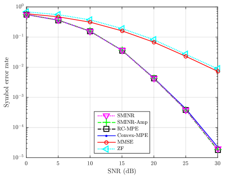
Figure 1: Average symbol error rates of users for $N=4$ receive antennas and $K=4$ users with 8-PAM modulation.

Fig. 1 compares the average symbol error rates of classical ZF and MMSE receive beamforming with the proposed MPE, reduced-complexity MPE (RC-MPE), amplitude version of maximum SMINR (SMINR-Amp), and heuristic maximum SMINR (SMINR) beamforming. As expected, all the proposed methods substantially outperform ZF and MMSE beamforming. For example, at a symbol error rate of $2.3\times 10^{-2}$, all the proposed beamforming methods show a gain of about 9 dB compared to that of ZF and MMSE beamforming. It is interesting to observe that average error probability of users is nearly the same for all the proposed receive beamforming methods, at all SNRs. Based on Proposition 2, it is expected that convex MPE beamforming has the same performance as its reduced-complexity version, as confirmed in Fig. 1. However, it was not expected that the amplitude and heuristic versions of maximum SMINR perform as well as convex MPE beamforming. We expected these beamforming methods to perform slightly worse than convex MPE and RC-MPE beamforming, since they are designed based on minimization of an upper bound on the error probability. However, as can be seen in Fig. 1, maximum SMINR-Amp, at significantly lower complexity, shows nearly the same performance as that of convex MPE beamforming. This indicates that minimizing the proposed upper bound on the error probability of each user closely approximates minimization of the error probability function, at least in this example. Moreover, the near identical performance of the heuristic maximum SMINR beamforming to that of convex MPE beamforming also indicates that the SMINR function defined in (38) is an accurate reflection of the error probability function, again at least for this example.

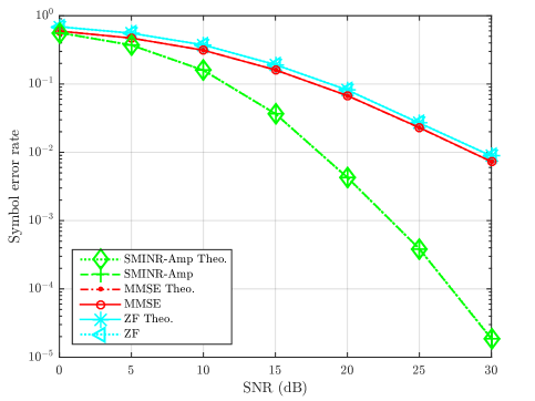
Figure 2: Average symbol error rates and theoretical symbol error rates of users for $N=4$ receive antennas and $K=4$ users with 8-PAM modulation.

Fig. 2 compares the average error probability of users using Monte Carlo simulation and their theoretical counterparts obtained by analytical expressions. Analytically calculated BER curves in this figure are obtained by substituting the calculated beamforming weights of users for each channel realization into the error probability function obtained in (III). As can be seen the calculated theoretical error probability precisely predicts the error performance of users.

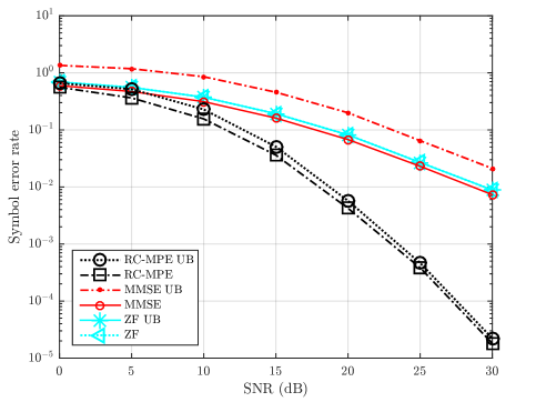
Figure 3: Symbol error rates and upper bounds on symbol error rates of users for $N=4$ receive antennas and $K=4$ users with 8-PAM modulation.

Fig. 3 compares the average error probability of users and their corresponding upper bounds given by (2). As can be seen, the upper bound curves are either above the error probability curves as in case of MMSE and RC-MPE beamforming or lie on top of the error probability curves as in case of ZF beamforming. In zero-forcing, the upper bound lies exactly over the error probability curve. In other words, in ZF beamforming the proposed upper bound on the error probability is equal to the exact error probability. The zero-forcing beamformer enforces the beamforming weight vector of a user to be orthogonal to the channels of other users, i.e., ${\bf w}_{k}{\bf h}_{j}=0,~{}k\neq j$. Therefore, in ZF beamforming the error probability (III) and the upper bound on the error probability (2) are equivalent. In Fig. 3, it can also be seen that at low SNRs the upper bound on error probability of MMSE beamforming is greater than one. This indicates that for the beamforming weights obtained by MMSE beamforming, the argument of the $Q$-function in (2) is not always greater than zero. It can also be seen that in reduced-complexity MPE beamforming, the upper bound closely approximates the error probability. Overall, based on Fig. 3, it is inferred that the tightness of the proposed upper bound is not the same for different beamforming techniques but depends on the values of the beamforming weight vectors of the users.

Figure 4: Average sum rates when $N=4$ and $K=2$ with 64-QAM modulated signals for ZF-QAM and MMSE-QAM and when $N=4$ and $K=4$ with 8-PAM modulated signals for the other simulated beamforming methods.

So far, we have compared the proposed beamforming techniques for 1D signalling with classical beamforming using 1D signalling. It would also be instructive to extend the above comparison to two-dimensionally modulated signals. Fig. 4 compares the expected sum rate (throughput) of users employing the proposed beamforming methods of one-dimensionally modulated signals and classical beamforming of both one-dimensionally and two-dimensionally modulated signals. As can be seen, at all SNRs, the proposed convex-MPE, RC-MPE, maximum SMINR-Amp, and maximum SMINR beamforming methods achieve higher sum rates than ZF and MMSE beamforming. It should be remarked that in addition to the sum rate of four users with 8-PAM modulation and the proposed beamforming methods, the sum rate of two users with 64-QAM modulation using ZF and MMSE receive beamforming are also included in Fig. 4. Theoretically, four users with 8-PAM signalling as well as two users with 64-QAM signalling achieve a maximum bit rate of 12 bits/channel use. Therefore, it is interesting to observe that the proposed beamforming methods which are developed for one-dimensionally modulated signals not only outperform classical beamforming of one-dimensionally modulated signals (as expected), but also they outperform classical beamforming of their counterpart two-dimensional modulations.

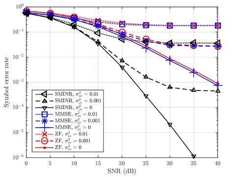
Figure 5: Average symbol error rates of users for $N=4$ receive antennas and $K=4$ users with 8-PAM modulation assuming imperfect CSI.

As has been seen so far, power-based maximum SMINR beamforming with closed-form solution exhibits superior performance compared to conventional ZF and MMSE beamforming. Therefore, it would be interesting to compare its sensitivity to imperfect CSI with that of ZF and MMSE beamforming. In Fig. 5, average symbol error rates of users assuming both perfect and imperfect CSI are presented for maximum SMINR, ZF, and MMSE beamforming. For imperfect CSI, it is assumed that channel estimation error is normally distributed with zero mean and variance of either $\sigma_{ce}^{2}=0.01$ or $0.001$. As mentioned earlier, the channel gains have a CSCG distribution with zero mean and unit variance. It is seen in Fig. 5 that as estimation error increases, the error probability increases. In this figure and also in Fig. 1, it can be seen that the proposed maximum SMINR beamforming with perfect CSI outperforms ZF and MMSE beamforming methods with perfect CSI. In Fig. 5, it is observed that the proposed maximum SMINR beamforming with imperfect CSI also outperforms classical beamforming methods with imperfect CSI. For example, from Fig. 5, at SNR of 40 dB and channel error variance of $\sigma_{ce}^{2}=0.001$, bit error error rate of maximum SMINR beamforming is $4.5\times 10^{-4}$, while bit error rates of ZF and MMSE beamforming are about $2.7\times 10^{-2}$. It is interesting to note that up to SNR of 40 dB, the maximum SMINR with $\sigma_{ce}^{2}=0.001$ not only outperforms both ZF and MMSE with $\sigma_{ce}^{2}=0.001$ but also outperforms ZF and MMSE with perfect CSI.

VII Conclusion

In this paper, it has been shown that by exploiting the type of modulation in the design of receive beamforming, the performance of a multiuser multiple-access communications system can be tremendously improved. The error probability of each user can be calculated and minimized to obtain the optimum beamforming weights. This highly nonlinear optimization problem was transformed to a convex optimization problem and two reduced-complexity versions of the problem were also introduced and solved numerically. Finally, the error probability in a multiuser scenario resulted in the development of a new metric called signal minus interference to noise ratio, where its maximization resulted in a closed-form solution for receive beamforming weights based on a simple eigenvalue decomposition. It has been shown that all the proposed beamforming techniques outperform the classical zero-forcing and MMSE beamforming.

Appendix A Proof of Proposition 1

Assume that there exists a $b=b_{1}$ such that

$$\Re\{{\bf w}_{k}{\bf h}_{k}d\sqrt{E_{g}}-{\bf w}_{k}{\bf H}_{\bar{k}}{\bf s}_{\bar{k}}(b_{1})\}<0.$$ (49)

Therefore,

$$\frac{\Re\{{\bf w}_{k}{\bf h}_{k}d\sqrt{E_{g}}-{\bf w}_{k}{\bf H}_{\bar{k}}{\bf s}_{\bar{k}}(b_{1})\}}{\frac{\sigma_{z}}{\sqrt{2}}\|{\bf w}_{k}\|_{2}}<0.$$ (50)

Hence,

$$Q\left(\frac{\Re\{{\bf w}_{k}{\bf h}_{k}d\sqrt{E_{g}}-{\bf w}_{k}{\bf H}_{\bar{k}}{\bf s}_{\bar{k}}(b_{1})\}}{\frac{\sigma_{z}}{\sqrt{2}}\|{\bf w}_{k}\|_{2}}\right)>\frac{1}{2}.$$ (51)

Consequently, error probability is written as

$$P_{e_{k}}=\frac{L_{k}-1}{N_{b}}$$

$$+\frac{2(L_{k}-1)}{N_{b}}\sum_{\begin{subarray}{c}b=1\\ b\neq b_{1}\end{subarray}}^{N_{p_{k}}}Q\left(\frac{\Re\{{\bf w}_{k}{\bf h}_{k}d\sqrt{E_{g}}-{\bf w}_{k}{\bf H}_{\bar{k}}{\bf s}_{\bar{k}}(b)\}}{\frac{\sigma_{z}}{\sqrt{2}}\|{\bf w}_{k}\|_{2}}\right).$$ (52)

If $d\sqrt{E_{g}}$ approaches infinity, error probability of user $k$ approaches $\lim_{d\sqrt{E_{g}}\rightarrow+\infty}P_{e_{k}}=\frac{L_{k}-1}{N_{b}}$. In other words, there always exists an error floor of $\frac{L_{k}-1}{KN_{b}}=\frac{L_{k}-1}{L_{k}N_{p}K}$, because the number of users is limited and consequently is $N_{p}$.

Appendix B Proof of Property 2

Let ${\bf w}^{\prime}_{k}=c{\bf w}_{k}$, where $c\in\mathbb{R}^{+}$. We have

$$P_{e_{k}}({\bf w}^{\prime}_{k})$$

$$=\frac{2(L_{k}-1)}{N_{b}}\sum_{b=1}^{N_{p_{k}}}Q\left(\frac{\Re\{{\bf w}^{\prime}_{k}{\bf h}_{k}d\sqrt{E_{g}}-{\bf w}^{\prime}_{k}{\bf H}_{\bar{k}}{\bf s}_{\bar{k}}(b)\}}{\frac{\sigma_{z}}{\sqrt{2}}\|{\bf w}^{\prime}_{k}\|_{2}}\right)$$

$$=\frac{2(L_{k}-1)}{N_{b}}\sum_{b=1}^{N_{p_{k}}}Q\!\left(\!\frac{\Re\{c{\bf w}_{k}{\bf h}_{k}d\sqrt{E_{g}}\!-\!c{\bf w}_{k}{\bf H}_{\bar{k}}{\bf s}_{\bar{k}}(b)\}}{\frac{\sigma_{z}}{\sqrt{2}}\|c{\bf w}_{k}\|_{2}}\!\right)$$

$$=P_{e_{k}}({\bf w}_{k}).$$ (53)

Appendix C Proof of Theorem 1

The minimization problem of error probability of user $k$ is considered over the following feasible set:

$${\mathcal{F}}_{k}= \{{\bf w}_{k}|{\bf w}_{k}{\bf w}_{k}^{H}=1\wedge~{}$$

$$\Re\{{\bf w}_{k}{\bf h}_{k}d\sqrt{E_{g}}-{\bf w}_{k}{\bf H}_{\bar{k}}{\bf s}_{\bar{k}}(b)\}\geq 0,~{}1\leq b\leq N_{p_{k}}\}.$$ (54)

Assume that ${\bf w}_{k_{1}}\in{\mathcal{F}}_{k}$ is a global minimizer of the optimization problem (28), and ${\bf w}_{k_{2}}\in{\mathcal{F}}_{k}$ is a local minimizer of the problem such that

$$P_{e_{k}}({\bf w}_{k_{1}})<P_{e_{k}}({\bf w}_{k_{2}}).$$ (55)

Assuming $0<\alpha<1$, we define ${\bf w}_{k_{0}}$ as

$${\bf w}_{k_{0}}=\frac{\alpha{\bf w}_{k_{1}}+(1-\alpha){\bf w}_{k_{2}}}{\|\alpha{\bf w}_{k_{1}}+(1-\alpha){\bf w}_{k_{2}}\|_{2}}.$$ (56)

Therefore, we have $\|{\bf w}_{k_{0}}\|=1$, and for $1\leq b\leq N_{p_{k}}$, we have $\Re\{{\bf w}_{k_{0}}{\bf h}_{k}d\sqrt{E_{g}}-{\bf w}_{k_{0}}{\bf H}_{\bar{k}}{\bf s}_{\bar{k}}(b)\}\geq 0$. Hence, it can be inferred that ${\bf w}_{k_{0}}\in{\mathcal{F}}_{k}$. It is also obvious that

$$\|\alpha{\bf w}_{k_{1}}+(1-\alpha){\bf w}_{k_{2}}\|_{2}\leq\alpha\|{\bf w}_{k_{1}}\|_{2}+(1-\alpha)\|{\bf w}_{k_{2}}\|_{2}=1.$$ (57)

Consequently,

$$\Re\{{\bf w}_{k_{0}}{\bf h}_{k}d\sqrt{E_{g}}-{\bf w}_{k_{0}}{\bf H}_{\bar{k}}{\bf s}_{\bar{k}}(b)\}$$

$$\geq\alpha\Re\{{\bf w}_{k_{1}}{\bf h}_{k}d\sqrt{E_{g}}-{\bf w}_{k_{1}}{\bf H}_{\bar{k}}{\bf s}_{\bar{k}}(b)\}$$

$$+(1-\alpha)\Re\{{\bf w}_{k_{2}}{\bf h}_{k}d\sqrt{E_{g}}-{\bf w}_{k_{2}}{\bf H}_{\bar{k}}{\bf s}_{\bar{k}}(b)\},~{}1\leq b\leq N_{p_{k}}.$$ (58)

Therefore, we have

$$Q\left(\frac{\Re\{{\bf w}_{k_{0}}{\bf h}_{k}d\sqrt{E_{g}}-{\bf w}_{k_{0}}{\bf H}_{\bar{k}}{\bf s}_{\bar{k}}(b)\}}{\frac{\sigma_{z}}{\sqrt{2}}}\right)$$

$$\leq Q\left(\frac{\alpha\Re\{{\bf w}_{k_{1}}{\bf h}_{k}d\sqrt{E_{g}}-{\bf w}_{k_{1}}{\bf H}_{\bar{k}}{\bf s}_{\bar{k}}(b)\}+(1-\alpha)\Re\{{\bf w}_{k_{2}}{\bf h}_{k}d\sqrt{E_{g}}-{\bf w}_{k_{2}}{\bf H}_{\bar{k}}{\bf s}_{\bar{k}}(b)\}}{\frac{\sigma_{z}}{\sqrt{2}}}\right)$$

$$\leq\alpha Q\left(\frac{\Re\{{\bf w}_{k_{1}}{\bf h}_{k}d\sqrt{E_{g}}-{\bf w}_{k_{1}}{\bf H}_{\bar{k}}{\bf s}_{\bar{k}}(b)\}}{\frac{\sigma_{z}}{\sqrt{2}}}\right)$$

$$+(1-\alpha)Q\left(\frac{\Re\{{\bf w}_{k_{2}}{\bf h}_{k}d\sqrt{E_{g}}-{\bf w}_{k_{2}}{\bf H}_{\bar{k}}{\bf s}_{\bar{k}}(b)\}}{\frac{\sigma_{z}}{\sqrt{2}}}\right),\quad 1\leq b\leq N_{p_{k}},$$ (59)

where the first inequality results from (C) and due to the fact that $Q(x)$ is a decreasing function for $x\geq 0$, and the second inequality stands because $Q(x)$ is a convex function for $x\geq 0$.

From (III) and (C), it can be inferred that

$$P_{e_{k}}({\bf w}_{k_{0}})$$

$$=\frac{2(L_{k}-1)}{N_{b}}\sum_{b=1}^{N_{p_{k}}}Q\left(\frac{\Re\{{\bf w}_{k_{0}}{\bf h}_{k}d\sqrt{E_{g}}-{\bf w}_{k_{0}}{\bf H}_{\bar{k}}{\bf s}_{\bar{k}}(b)\}}{\frac{\sigma_{z}}{\sqrt{2}}\|{\bf w}_{k_{0}}\|_{2}}\right)$$

$$\leq\frac{\alpha 2(L_{k}-1)}{N_{b}}\sum_{b=1}^{N_{p_{k}}}Q\left(\frac{\Re\{{\bf w}_{k_{1}}{\bf h}_{k}d\sqrt{E_{g}}-{\bf w}_{k_{1}}{\bf H}_{\bar{k}}{\bf s}_{\bar{k}}(b)\}}{\frac{\sigma_{z}}{\sqrt{2}}\|{\bf w}_{k_{1}}\|_{2}}\right)$$

$$+\!\frac{(1\!-\!\alpha)2(L_{k}\!-\!1)}{N_{b}}\!\sum_{b=1}^{N_{p_{k}}}\!\!Q\!\left(\!\frac{\Re\{\!{\bf w}_{k_{2}}{\bf h}_{k}d\sqrt{E_{g}}\!-\!{\bf w}_{k_{2}}{\bf H}_{\bar{k}}{\bf s}_{\bar{k}}(b)\!\}}{\frac{\sigma_{z}}{\sqrt{2}}\|{\bf w}_{k_{2}}\|_{2}}\!\right)$$

$$=\!\alpha P_{e_{k}}({\bf w}_{k_{1}})\!+\!(1\!-\!\alpha)P_{e_{k}}({\bf w}_{k_{2}})\!<\!P_{e_{k}}({\bf w}_{k_{2}}),~{}\forall\alpha\!\in\!(0,1),$$ (60)

where the last inequality is due to the assumption of the proof, i.e., ${\bf w}_{k_{1}}$ is the global minimizer of $P_{e_{k}}$. Now, let $\alpha\rightarrow 0$, ${\bf w}_{k_{0}}\rightarrow{\bf w}_{k_{2}}$. Hence, in a small neighborhood of ${\bf w}_{k_{2}}$, there always exists a ${\bf w}_{k_{0}}$, so that $P_{e_{k}}({\bf w}_{k_{0}})<P_{e_{k}}({\bf w}_{k_{2}})$, i.e., ${\bf w}_{k_{2}}$ is not a local minimizer. In other words, there does not exist any local minimizer such that (55) holds. Therefore, it can be concluded that either no local minimizer exists, which proves the theorem, or there exists a local minimizer such that $P_{e_{k}}({\bf w}_{k_{1}})\geq P_{e_{k}}({\bf w}_{k_{2}})$. However, since ${\bf w}_{k_{1}}$ is a global minimizer of $P_{e_{k}}({\bf w}_{k})$, we have $P_{e_{k}}({\bf w}_{k_{1}})\leq P_{e_{k}}({\bf w}_{k_{2}})$. Therefore, it can be concluded that $P_{e_{k}}({\bf w}_{k_{1}})=P_{e_{k}}({\bf w}_{k_{2}})$, i.e., the local minimizer (if exists) is also a global minimizer.

To show the uniqueness of the global minimizer, first we consider the following set:

$${\mathcal{F}}_{k}^{0}= \{{\bf w}_{k}|{\bf w}_{k}{\bf w}_{k}^{H}=1\wedge~{}$$

$$\Re\{{\bf w}_{k}{\bf h}_{k}d\sqrt{E_{g}}-{\bf w}_{k}{\bf H}_{\bar{k}}{\bf s}_{\bar{k}}(b)\}=0,~{}1\leq b\leq N_{p_{k}}\}.$$ (61)

It is obvious that each point in this set is a global maximizer of error probability function in (III) constrained by the set defined in (C), because the arguments of all $Q$-functions in error probability (III) will be zero. Therefore, to solve the minimization problem it is sufficient to solve the problem over the set ${\mathcal{F}}_{k}^{1}={\mathcal{F}}_{k}-{\mathcal{F}}_{k}^{0}$. The error probability of user $k$, $P_{e_{k}}({\bf w}_{k})$, is strictly convex on ${\mathcal{F}}_{k}^{1}$, because $Q(x)$ is strictly convex for $x>0$. Assume that ${\bf w}_{k_{1}}\neq{\bf w}_{k_{2}}$ are two global minimizers of the optimization problem (28). We define ${\bf w}_{k_{0}}$ as follows:

$${\bf w}_{k_{0}}=\frac{\alpha{\bf w}_{k_{1}}+(1-\alpha){\bf w}_{k_{2}}}{\|\alpha{\bf w}_{k_{1}}+(1-\alpha){\bf w}_{k_{2}}\|_{2}},\quad\forall\alpha\in(0,1).$$ (62)

Since ${\bf w}_{k_{1}}$ is a global minimizer, it is obvious that

$$P_{e_{k}}({\bf w}_{k_{0}})\geq P_{e_{k}}({\bf w}_{k_{1}}).$$ (63)

On the other hand, we have

$$P_{e_{k}}({\bf w}_{k_{0}})<\alpha P_{e_{k}}({\bf w}_{k_{1}})+(1-\alpha)P_{e_{k}}({\bf w}_{k_{2}})=P_{e_{k}}({\bf w}_{k_{1}}),$$ (64)

because $P_{e_{k}}({\bf w}_{k})$ is strictly convex on ${\mathcal{F}}_{k}^{1}$. Since (64) contradicts (63), it can be inferred that the global minimizer is unique.

Appendix D Proof of Proposition 2

To prove this proposition we first prove the sufficient condition by showing that the left hand side (LHS) of (32) is a lower bound on the LHS of the inequality (31c) for all $b$.

For $1\leq j,k\leq K$, we have

$$|\Re\{{\bf w}_{k}{\bf h}_{j}s_{j}(L_{j})\}|=|\Re\{{\bf w}_{k}{\bf h}_{j}\}|.|s_{j}(L_{j})|$$

$$\geq|\Re\{{\bf w}_{k}{\bf h}_{j}\}|.|s_{j}(l_{j})|\geq\Re\{{\bf w}_{k}{\bf h}_{j}\}s_{j}(l_{j})$$

$$=\Re\{{\bf w}_{k}{\bf h}_{j}s_{j}(l_{j})\},\quad\forall l_{j}\in\{1,\cdots,L_{j}\}.$$ (65)

Therefore,

$$\sum_{\begin{subarray}{c}j=1\\ j\neq k\end{subarray}}|\Re\{{\bf w}_{k}{\bf h}_{j}s_{j}(L_{j})\}|\geq\sum_{\begin{subarray}{c}j=1\\ j\neq k\end{subarray}}\Re\{{\bf w}_{k}{\bf h}_{j}s_{j}(l_{j})\}$$ (66)

$$=\Re\{{\bf w}_{k}{\bf H}_{\bar{k}}{\bf s}_{\bar{k}}(b)\},\quad 1\leq b\leq N_{p_{k}}.$$

Hence,

$$\Re\{{\bf w}_{k}{\bf h}_{k}d\sqrt{E_{g}}\}-\sum_{\begin{subarray}{c}j=1\\ j\neq k\end{subarray}}^{K}|\Re\{{\bf w}_{k}{\bf h}_{j}s_{j}(L_{j})\}|$$

$$\leq\Re\{{\bf w}_{k}{\bf h}_{k}d\sqrt{E_{g}}\}-\Re\{{\bf w}_{k}{\bf H}_{\bar{k}}{\bf s}_{\bar{k}}(b)\}$$

$$=\Re\{{\bf w}_{k}{\bf h}_{k}d\sqrt{E_{g}}-{\bf w}_{k}{\bf H}_{\bar{k}}{\bf s}_{\bar{k}}(b)\},\quad 1\leq b\leq N_{p_{k}}.$$ (67)

Thus, if $\Re\{{\bf w}_{k}{\bf h}_{k}d\sqrt{E_{g}}\}-\sum_{\begin{subarray}{c}j=1\\ j\neq k\end{subarray}}^{K}|\Re\{{\bf w}_{k}{\bf h}_{j}s_{j}(L_{j})\}|\geq 0$ then $\Re\{{\bf w}_{k}{\bf h}_{k}d\sqrt{E_{g}}-{\bf w}_{k}{\bf H}_{\bar{k}}\allowbreak{\bf s}_{\bar{k}}(b)\}\geq 0,~{}1\leq b\leq N_{p_{k}}$.

To prove the necessary condition, we use contradiction. Let us assume that $\Re\{{\bf w}_{k}{\bf h}_{k}d\sqrt{E_{g}}\}-\sum_{\begin{subarray}{c}j=1\\ j\neq k\end{subarray}}^{K}|\Re\{{\bf w}_{k}{\bf h}_{j}s_{j}(L_{j})\}|<0$. Therefore, we have

$$\Re\{{\bf w}_{k}{\bf h}_{k}d\sqrt{E_{g}}\}-\sum_{\begin{subarray}{c}j=1\\ j\neq k\end{subarray}}^{K}|\Re\{{\bf w}_{k}{\bf h}_{j}s_{j}(L_{j})\}|$$

$$=\Re\{{\bf w}_{k}{\bf h}_{k}d\sqrt{E_{g}}\}-\sum_{\begin{subarray}{c}j=1\\ j\neq k\end{subarray}}^{K}\Re\{{\bf w}_{k}{\bf h}_{j}\}\operatorname{sgn}(\Re\{{\bf w}_{k}{\bf h}_{j}\})s_{j}(L_{j})$$

$$=\Re\{{\bf w}_{k}{\bf h}_{k}d\sqrt{E_{g}}\}-\sum_{\begin{subarray}{c}j=1\\ j\neq k\end{subarray}}^{K}\Re\{{\bf w}_{k}{\bf h}_{j}\}s_{j}(\ell_{j})$$

$$=\Re\{{\bf w}_{k}{\bf h}_{k}d\sqrt{E_{g}}\}-\Re\{{\bf w}_{k}{\bf H}_{\bar{k}}{\bf s}_{\bar{k}}(\beta)\}<0,$$ (68)

where ${\bf s}_{\bar{k}}(\beta)=[s_{1}(\ell_{1}),\cdots,s_{k-1}(\ell_{k-1}),s_{k+1}(\ell_{k+1}),\cdots,\allowbreak s_{K}(\ell_{K})]^{T}$, and for $j\neq k$, $\ell_{j}=L_{j}$ if $\operatorname{sgn}(\Re\{{\bf w}_{k}{\bf h}_{j}\})=1$ and $\ell_{j}=1$ if $\operatorname{sgn}(\Re\{{\bf w}_{k}{\bf h}_{j}\})=-1$. Therefore, there exists a $b=\beta$ such that $\Re\{{\bf w}_{k}{\bf h}_{k}d\sqrt{E_{g}}\}\allowbreak-\Re\{{\bf w}_{k}{\bf H}_{\bar{k}}{\bf s}_{\bar{k}}(\beta)\}<0$, i.e., at least one constraint in (31c) is not satisfied.

Appendix E Proof of Claim 1

Using the definition of a convex set [32], it is assumed that ${\bf w}_{k_{1}}$ and ${\bf w}_{k_{2}}$ are two arbitrary points in the set defined by (33c), i.e.,

$$\{{\bf w}_{k}|\Re\{{\bf w}_{k}{\bf h}_{k}d\sqrt{E_{g}}\}-\sum_{\begin{subarray}{c}j=1\\ j\neq k\end{subarray}}^{K}\left|\Re\{{\bf w}_{k}{\bf h}_{j}s_{j}(L_{j})\}\right|\geq 0\}.$$ (69)

For any $0\leq\alpha\leq 1$,

$$|\Re\{(\alpha{\bf w}_{k_{1}}+(1-\alpha){\bf w}_{k_{2}}){\bf h}_{j}s_{j}(L_{j})\}|$$

$$=|\alpha\Re\{{\bf w}_{k_{1}}{\bf h}_{j}s_{j}(L_{j})\}+(1-\alpha)\Re\{{\bf w}_{k_{2}}{\bf h}_{j}s_{j}(L_{j})\}|$$

$$\leq|\alpha\Re\{{\bf w}_{k_{1}}{\bf h}_{j}s_{j}(L_{j})\}|+|(1-\alpha)\Re\{{\bf w}_{k_{2}}{\bf h}_{j}s_{j}(L_{j})\}|$$

$$=\alpha|\Re\{{\bf w}_{k_{1}}{\bf h}_{j}s_{j}(L_{j})\}|+(1-\alpha)|\Re\{{\bf w}_{k_{2}}{\bf h}_{j}s_{j}(L_{j})\}|,$$ (70)

where the inequality is the result of the triangle inequality. Therefore,

$$\sum_{\begin{subarray}{c}j=1\\ j\neq k\end{subarray}}^{K}|\Re\{(\alpha{\bf w}_{k_{1}}+(1-\alpha){\bf w}_{k_{2}}){\bf h}_{j}s_{j}(L_{j})\}|$$

$$\leq\!\sum_{\begin{subarray}{c}j=1\\ j\neq k\end{subarray}}^{K}\alpha|\Re\{{\bf w}_{k_{1}}{\bf h}_{j}s_{j}(L_{j})\}|\!+\!\sum_{\begin{subarray}{c}j=1\\ j\neq k\end{subarray}}^{K}(1\!-\!\alpha)|\Re\{{\bf w}_{k_{2}}{\bf h}_{j}s_{j}(L_{j})\}|,$$ (71)

and consequently,

$$\Re\{(\alpha{\bf w}_{k_{1}}+(1-\alpha){\bf w}_{k_{2}}){\bf h}_{k}d\sqrt{E_{g}}\}$$

$$-\sum_{\begin{subarray}{c}j=1\\ j\neq k\end{subarray}}^{K}|\Re\{(\alpha{\bf w}_{k_{1}}+(1-\alpha){\bf w}_{k_{2}}){\bf h}_{j}s_{j}(L_{j})\}|$$

$$\geq\alpha\left(\Re\{{\bf w}_{k_{1}}{\bf h}_{k}d\sqrt{E_{g}}\}-\sum_{\begin{subarray}{c}j=1\\ j\neq k\end{subarray}}^{K}|\Re\{{\bf w}_{k_{1}}{\bf h}_{j}s_{j}(L_{j})\}|\right)$$

$$+(1-\alpha)\left(\Re\{{\bf w}_{k_{2}}{\bf h}_{k}d\sqrt{E_{g}}\}-\sum_{\begin{subarray}{c}j=1\\ j\neq k\end{subarray}}^{K}|\Re\{{\bf w}_{k_{2}}{\bf h}_{j}s_{j}(L_{j})\}|\right)$$

$$\geq 0.$$ (72)

The last inequality holds because ${\bf w}_{k_{1}}$ and ${\bf w}_{k_{2}}$ are in the set (69). Thus, (33c) is a convex set.

References

• [1] I. E. Telatar, “Capacity of multi-antenna Gaussian channels,” European Trans. Telecommun., vol. 10, no. 6, pp. 585–595, Nov. 1999.
• [2] A. J. Paulraj, D. A. Gore, R. U. Nabar, and H. Bolcskei, “An overview of MIMO communications - A key to gigabit wireless,” Proc. IEEE, vol. 92, no. 2, pp. 198–218, Feb. 2004.
• [3] D. Gesbert, M. Kountouris, R. W. Heath Jr., C.-B. Chae, and T. Sälzer, “From single-user to multiuser communications: Shifting the MIMO paradigm,” IEEE Signal Process. Mag., vol. 24, no. 5, pp. 36–46, Sep. 2007.
• [4] W. Yu and J. M. Cioffi, “Sum capacity of Gaussian vector broadcast channels,” IEEE Trans. Inf. Theory, vol. 50, no. 9, pp. 1875–1892, Sep. 2004.
• [5] C. Lim, T. Yoo, B. Clerckx., B. Lee, and B. Shim, “Recent trend of multiuser MIMO in LTE-Advanced,” IEEE Commun. Mag., vol. 51, no. 3, pp. 127–135, Mar. 2013.
• [6] B. D. V. Veen and K. M. Buckley, “Beamforming: A versatile approach to spatial filtering,” Proc. IEEE, vol. 5, pp. 4–24, Apr 1988.
• [7] J. Litva and T. K. Y. Lo, Digital Beamforming in Wireless Communications.   London, U.K.: Artech, 1996.
• [8] N. D. Sidiropoulos, T. N. Davidson, and Z.-Q. Luo, “Transmit beamforming for physical-layer multicasting,” IEEE Trans. Signal Process., vol. 54, no. 6, pp. 2239–2251, Jun. 2006.
• [9] A. B. Gershman, N. D. Sidiropoulos, S. Shahbazpanahi, M. Bengtsson, and B. Ottersten, “Convex optimization-based beamforming,” IEEE Signal Process. Mag., vol. 27, no. 3, pp. 62–75, May 2010.
• [10] M. Bavand and P. Azmi, “Successive detection based minimum probability of error beamforming,” in Proc. 18th IEEE Int. Conf. Telecommun., May 2011, pp. 357–362.
• [11] L. C. Godara, “Applications of antenna arrays to mobile communications, Part I: performance improvement, feasibility, and system considerations,” Proc. IEEE, vol. 85, no. 7, pp. 1031 –1060, Jul. 1997.
• [12] ——, “Application of antenna arrays to mobile communications, Part II: Beam-forming and direction-of-arrival considerations,” Proc. IEEE, vol. 85, no. 8, pp. 1195–1245, Aug. 1997.
• [13] L. Liu, R. Chen, S. Geirhofer, K. Sayana, Z. Shi, and Y. Zhou, “Downlink MIMO in LTE-advanced: SU-MIMO vs. MU-MIMO,” IEEE Commun. Mag., vol. 50, no. 2, pp. 140–147, Feb. 2012.
• [14] I. N. Psaromiligkos, S. N. Batalama, and D. A. Pados, “On adaptive minimum probability of error linear filter receivers for DS-CDMA channels,” IEEE Trans. Commun., vol. 47, no. 7, pp. 1092–1102, Jul. 1999.
• [15] N. Wang and S. D. Blostein, “Approximate minimum BER power allocation for MIMO spatial multiplexing systems,” IEEE Trans. Commun., vol. 55, no. 1, pp. 180–187, Jan. 2007.
• [16] ——, “Minimum BER transmit power allocation and beamforming for two-input multiple-output spatial multiplexing systems,” IEEE Trans. Veh. Technol., vol. 56, no. 2, pp. 704–709, Mar. 2007.
• [17] Q. Z. Ahmed, M.-S. Alouini, and S. Aissa, “Bit error-rate minimizing detector for amplify-and-forward relaying systems using generalized Gaussian kernel,” IEEE Signal Process. Lett., vol. 20, no. 1, pp. 55–58, Jan. 2013.
• [18] C.-C. Yeh and J. R. Barry, “Approximate minimum bit-error rate equalization for binary signaling,” in Proc. IEEE Int. Conf. Commun. (ICC), 1997, pp. 1095–1099.
• [19] C. C. Yeh and J. R. Barry, “Adaptive minimum bit-error rate equalization for binary signaling,” IEEE Trans. Commun., vol. 48, no. 7, pp. 1226–1235, Jul. 2000.
• [20] X. Wang, W.-S. Lu, and A. Antoniou, “Constrained minimum-BER multiuser detection,” IEEE Trans. Signal Process., vol. 48, no. 10, pp. 2903–2909, Oct. 2000.
• [21] J. Li, G. Wei, and F. Chen, “On minimum-BER linear multiuser detection for DS-CDMA channels,” IEEE Trans. Signal Process., vol. 55, no. 3, pp. 1093–1103, Mar. 2007.
• [22] S. Chen, N. N. Ahmad, and L. Hanzo, “Adaptive minimum bit error rate beamforming,” IEEE Trans. Wireless Commun., vol. 4, no. 2, pp. 341–348, Mar. 2005.
• [23] S. Chen, A. Livingstone, H.-Q. Du, and L. Hanzo, “Adaptive minimum symbol error rate beamforming assisted detection for quadrature amplitude modulation,” IEEE Trans. Wireless Commun., vol. 7, no. 4, pp. 1140–1145, Apr. 2008.
• [24] M. Bavand, P. Azmi, and S. D. Blostein, “Convex optimization based minimum probability of error beamforming in the uplink of a multiuser system,” in Proc. IEEE 27th Biennial Symp. Commun. (QBSC), Jun. 2014, pp. 28–32.
• [25] “Emerging communication technologies enabling the Internet of things,” Rohde & Schwarz White Paper, Sep. 2016.
• [26] “LTE-M - optimizing LTE for the Internet of things,” Nokia Network White Paper, 2015.
• [27] S. Abdallah and S. D. Blostein, “Rate adaptation using long range channel prediction based on discrete prolate spheroidal sequences,” in Proc. IEEE 15th Int. Workshop Signal. Process. Adv. Wireless Commun. (SPAWC), Jun. 2014, pp. 479–483.
• [28] G. D. Forney Jr. and G. Ungerboeck, “Modulation and coding for linear Gaussian channels,” IEEE Trans. Inf. Theory, vol. 44, no. 6, pp. 2384–2415, Oct. 1998.
• [29] A. Paulraj, R. Nabar, and D. Gore, Introduction to Space-Time Wireless Communications.   Cambridge University Press, 2003.
• [30] J. Mao, J. Gao, Y. Liu, and G. Xie, “Simplified semi-orthogonal user selection for MU-MIMO systems with ZFBF,” IEEE Wireless Commun. Lett., vol. 1, no. 1, pp. 42–45, Feb. 2012.
• [31] J. Nocedal and S. J. Wright, Numerical Optimization, 2nd ed.   New York, USA: Springer, 2006.
• [32] S. Boyd, Convex Optimization.   Cambridge University Press, 2004.
• [33] D. Brandwood, “A complex gradient operator and its application in adaptive array theory,” Proc. IEEE, vol. 130, no. 1, pp. 11–16, Feb. 1983.
• [34] A. Hjørungnes and D. Gesbert, “Complex-valued matrix differentiation: Techniques and key results,” IEEE Trans. Signal Process., vol. 55, no. 6, pp. 2740–2746, Jun. 2007.
• [35] J. Eriksson, E. Ollila, and V. Koivunen, “Essential statistics and tools for complex random variables,” IEEE Trans. Signal Process., vol. 58, no. 10, pp. 5400–5408, Oct. 2010.
• [36] C. B. Peel, B. M. Hochwald, and A. L. Swindlehurst, “A vector-perturbation technique for near-capacity multiantenna multiuser communication-part I: Channel inversion and regularization,” IEEE Trans. Commun., vol. 53, no. 1, pp. 195–202, Jan. 2005.
• [37] M. Sadek, A. Tarighat, and A. H. Sayed, “A leakage-based precoding scheme for downlink multi-user MIMO channels,” IEEE Trans. Wireless Commun., vol. 6, no. 5, pp. 1711–1721, May 2007.