Theory of electron spin resonance in one-dimensional topological insulators with spin-orbit couplings: Detection of edge states

Abstract

Edge/surface states often appear in a topologically nontrivial phase when the system has a boundary. The edge state of a one-dimensional topological insulator is one of the simplest examples. Electron spin resonance (ESR) is an ideal probe to detect and analyze the edge state for its high sensitivity and precision. We consider ESR of the edge state of a generalized Su-Schrieffer-Heeger model with a next-nearest neighbor (NNN) hopping and a staggered spin-orbit coupling. The spin-orbit coupling is generally expected to bring about nontrivial changes on the ESR spectrum. Nevertheless, in the absence of the NNN hoppings, we find that the ESR spectrum is unaffected by the spin-orbit coupling thanks to the chiral symmetry. In the presence of both the NNN hopping and the spin-orbit coupling, on the other hand, the edge ESR spectrum exhibits a nontrivial frequency shift. We derive an explicit analytical formula for the ESR shift in the second-order perturbation theory, which agrees very well with a non-perturbative numerical calculation.

I Introduction

In recent decades, topological phases have become a central issue in condensed matter physics. An important class of topological phases is topological insulators and topological superconductors Hasan and Kane (2010); Qi and Zhang (2011); Bernevig and Hughes (2013); Shen (2013).

In condensed matter and statistical physics, one-dimensional (1-D) systems, which are amenable to several powerful analytical and numerical methods, often provide useful insights. 1-D topological phases are no exceptions. One of the simplest 1-D models possessing nontrivial topological nature is the Su-Schrieffer-Heeger (SSH) model Su et al. (1979), which has been used to describe the lattice structure of polyacetylene $[\text{C}_{2}\text{H}_{2}]_{\text{n}}$. The SSH model can be also applied to the 1-D charge density wave systems, such as quasi-one-dimensional conductors like TTF-TCNQ (tetrathiofulvalinium-tetracyanoquinodime- thanide) and KCP (potassium-tetracyanoplatinate) Schulz (1978). While the SSH model had been studied intensively much earlier than the notion of topological phases was conceived, there is a renewed interest from the viewpoint of topology. In fact, distinct phases of the SSH model are classified by the Zak phase Zak (1989) which is a topological invariant, and the bulk winding number of the momentum-space Hamiltonian Asbóth et al. (2016). In this sense, the SSH model can be regarded as a 1-D topological insulator.

An important nontrivial signature of many topological phases is edge states. The SSH model indeed possesses zero-energy edge states that are protected by a chiral symmetryAsbóth et al. (2016). The number of edge states at a domain wall is equal to the bulk winding number. This is known as the bulk-boundary correspondence in the spinless inversion-symmetric SSH modelAsbóth et al. (2016). Experimentally, 1-D systems with boundaries or edges can be realized by adding impurities to the material so that the system is broken to many finite chains. However, the edge states are often experimentally difficult to observe, since they are localized near the boundaries or the impurities and their contribution to bulk physical quantities is small. Given this challenge, electron spin resonance (ESR) provides one of the best methods to probe the edge states, thanks to its high sensitivity. In fact, the edge states of the $S=1$ Haldane chain were created by doping impurities and then successfully detected by ESR Hagiwara et al. (1990); Glarum et al. (1991). Furthermore, combined with near-edge x-ray absorption fine-structure experiments, ESR was applied successfully to probe the magnetic edge state in a graphene nanoribbon sample Joly et al. (2010); Campos-Delgado et al. (2008). Such a strategy could also be applied to 1-D topological insulators, which are described by the SSH model.

Another intriguing nature of ESR is that it is highly sensitive to magnetic anisotropies, such as the anisotropic exchange interaction, single-spin anisotropy, and the Dzyaloshinskii-Moriya (DM) interaction. The effect of magnetic anisotropies on ESR is well understood only in limited circumstances, and there remain many open issues Oshikawa and Affleck (1999, 2002). These magnetic anisotropies are often consequences of spin-orbit (SO) coupling which generally breaks spin-rotation symmetry. The effects of magnetic anisotropies and SO couplings also play important roles in magnetic dynamics in higher-dimensional topological phases Hasan and Kane (2010); Qi and Zhang (2011); Bernevig and Hughes (2013); Shen (2013); Shindou et al. (2010); Nakamura and Tokuno (2016). Thus it is of great interest to study the effect of SO coupling on ESR directly. However, this question has not been explored in much detail so far. An obstacle for the potential experimental ESR study of SO coupling is the electromagnetic screening in metallic systems. This problem does not exist in insulators. Unfortunately, band insulators are generally non-magnetic and we cannot expect interesting ESR properties. On the other hand, Mott insulators can have interesting magnetic properties. However, strong correlation effects, which are essential in Mott insulators, make theoretical analysis difficult.

In this context, the 1-D topological insulator provides a unique opportunity to study the effects of SO coupling on ESR. This would be of significant interest in several aspects. Experimentally, the insulating nature makes the observation of edge states by ESR easier. Theoretically, the interesting effects of anisotropic SO coupling on ESR can be studied accurately for the SSH model of non-interacting electrons. Moreover, the chiral symmetry, which is essential for the well-defined topological insulator phase, is often broken explicitly in realistic systems. When we introduce a chiral-symmetry breaking perturbation to the 1-D SSH model, the energy eigenvalues of the edge states generally deviate from zero energy. However, the edge states are expected to still survive and be localized near the edge if the perturbation is small enough. As we will demonstrate, the ESR of the edge state can detect the breaking of the chiral symmetry. The purpose of this paper is to present a theoretical analysis on ESR of the edge states in 1-D topological insulators, based on a generalized SSH model with SO couplings. We demonstrate several interesting aspects of ESR, which will hopefully stimulate corresponding experimental studies.

The paper is organized as follows. In Sec. II, we present the model of interest and review the basic topological nature of the SSH model. The next three sections are the main part of this paper. The properties of edge states are discussed in detail in Sec. III. In Sec. IV, we obtain a compact analytical formula of the ESR frequency shift in perturbation theory with respect to SO coupling. Section V is devoted to a direct numerical calculation of the ESR frequency shift, which is independent of the perturbative approach in Sec. IV. We find that the perturbation theory agrees with the numerical results very well. Finally, we present conclusions and future problems in Sec. VI.

II The model

II.1 A generalized SSH model

First let us consider a generalized SSH model with SO coupling

$${\mathscr{H}}_{0} = -\sum_{j=1}^{+\infty}\left\{t\left[1+(-1)^{j}\delta_{0}\right]c_{j+1}^{\dagger}\exp{\left[i(-1)^{j}\frac{\phi}{2}\vec{n}\cdot\vec{\sigma}\right]}c_{j}\right.$$ (1)

$$\left.+\text{h.c.}\right\}$$

where $c_{j}$ is the two-component electron annihilation operator $c_{j}\equiv[c_{j\uparrow},c_{j\downarrow}]^{T}$ at the $j$-th site, $t>0$ is the nearest-neighbor (NN) electron hopping amplitude, and $-1\leq\delta_{0}\leq 1$ is the bond-alternation parameter. The angle $\phi$ and axis $\vec{n}$ (which is a unit vector) parametrizes the SO coupling on the NN bond. The angle $\phi$ denotes the ratio of the SO coupling to the hopping amplitude on the bond. In this paper, we assume that $\phi$ is sufficiently small ($|\phi|\ll 1$), which is the case in many real materials. Expanding $\phi$ to first order, we obtain a standard form with so-called intrinsic and Rashba SO couplings Konschuh et al. (2010).

In our model Eq. (1), SO coupling is assumed to be staggered along the chain. This would be required, in the limit of $\delta_{0}=0$, if the system had site-centered inversion symmetry. In general, other forms of SO coupling including the uniform one along the chain are also possible. In this paper, however, we focus on the particular case of the staggered SO coupling to demonstrate its interesting effects on the ESR spectrum.

II.2 The SSH model and its topological properties

In the limit $\phi=0$, our model is reduced to the standard SSH model

$$\mathscr{H}_{\text{SSH}}=-\sum\left\{t\left[1+(-1)^{j}\delta_{0}\right]c_{j+1}^{\dagger}c_{j}+\text{h.c.}\right\}.$$ (2)

Let us first consider a system of $2N$ sites ($N$ unit cells) with the periodic boundary condition (PBC). It is then natural to take the momentum representation

$$c_{2j,\sigma} = \frac{1}{\sqrt{N}}\sum_{k}a_{k,\sigma}\exp{\left(ik(2j)\right)},$$ (3)

$$c_{2j+1,\sigma} = \frac{1}{\sqrt{N}}\sum_{k}b_{k,\sigma}\exp{\left(ik(2j+1)\right)},$$ (4)

where the summation of $k$ is in the reduced Brillouin zone $[0,\pi)$ with $k=n\pi/N$ and $n=0,\cdots,N-1$. Corresponding to the each sublattice (even and odd), there are two flavors of fermions, $a$ and $b$. The Hamiltonian can then be written as

$$\mathscr{H}_{\text{SSH}}=\sum_{k}(a_{k}^{\dagger},b_{k}^{\dagger}){h}_{\text{SSH}}(k)\begin{pmatrix}a_{k}\\ b_{k}\end{pmatrix},$$ (5)

with

$${h}_{\text{SSH}}(k)\equiv d_{x}(k)\tau_{x}+d_{y}(k)\tau_{y},$$ (6)

where $\tau_{x,y,z}$ are Pauli matrices acting on the flavor space, and $d_{x,y}(k)$ are real numbers

$$d_{x}(k)=-2t\cos(k);\,\,d_{y}(k)=2t\sin(k)\delta_{0}.$$ (7)

The spin indices are again suppressed in the Hamiltonian.

From this expression, the single-electron energy reads

$$\epsilon(k)=\pm\sqrt{{d_{x}(k)}^{2}+{d_{y}(k)}^{2}}=\pm 2t\sqrt{\cos^{2}{k}+{\delta_{0}}^{2}\sin^{2}{k}}.$$ (8)

The gap is closed at $k=\pi/2$ when $\delta_{0}=0$, while the system has a gap $4t|\delta_{0}|$ whenever the bond alternation does not vanish ($\delta_{0}\neq 0$). The gapless point can be regarded as a quantum critical point separating the two gapped phases, $\delta_{0}<0$ and $\delta_{0}>0$. Throughout this paper, we consider the half-filled case with $2N$ electrons. The bulk mode near this gap-closing point has a linear dispersion relation indicated in Fig. 1, and it can be described by a one-dimensional Dirac fermion Bernevig and Hughes (2013).

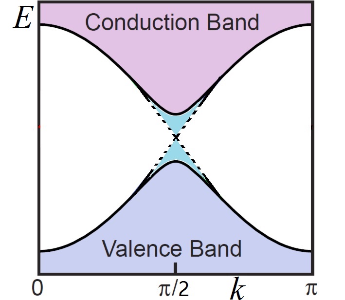
Figure 1: Band structure of the SSH model in Eq. (2) with a periodic boundary condition. Hasan and Kane (2010) The solid and dashed lines respectively represent band structures of the insulating case with $\delta_{0}\neq 0$ and the gapless point at $\delta_{0}=0$. The low-energy physics around $k=\pi/2$ can be described by one-dimensional Dirac fermion model.

It is evident from the Hamiltonian that each of the gapped phases is simply a dimerized phase. Nevertheless, we can identify them as a trivial insulator phase and a “topological insulator” phase. This can be understood by considering the system with the open boundary condition. Let us consider the chain of $2N$ sites labeled with $j=1,2,\ldots,2N$, and the open ends at sites $j=1$ and $2N$. For $\delta_{0}>0$ ($\delta_{0}<0$), sites $j=2n$ and $j=2n+1$ ($j=2n-1$ and $j=2n$) form a dimerized pair, respectively. As a consequence, for $\delta_{0}>0$ the end sites $j=1$ and $j=2N$ remain unpaired. The electrons at these unpaired sites give rise to $S=1/2$ edge states. In contrast, for $\delta_{0}<0$, there are no unpaired sites and thus no edge states. In this sense, $\delta_{0}>0$ is a topological insulator phase and $\delta_{0}<0$ is a trivial insulator phase. Of course, considering the equivalence of the two phases in the bulk, such a distinction involves an arbitrariness. That is, if we consider the an open chain of $N$ sites with $j=0,1,\ldots,2N-1$, the edge states appear only for $\delta_{0}<0$. It is still useful to identify the gapless point at $\delta_{0}=0$ as a quantum critical point separating the topological insulator and the trivial insulator phase.

The particular shape of the Hamiltonian also implies the existence of a chiral symmetry:

$$\{{h}_{\text{SSH}},\Gamma\}=0,$$ (9)

where $\Gamma\equiv\tau_{z}$. The chiral symmetry turns out to be important for the distinction of the two phases. In the context of the general classification of topological insulators, the present system corresponds to the “AIII” class with particle number conservation and the chiral symmetry in one spatial dimension Schnyder et al. (2008); Chiu et al. (2016).

In a general one dimensional free fermion system, we can define a topological invariant called the Zak phase Zak (1989) for each band as follows:

$$\gamma_{\text{Zak}}=i\oint_{\text{BZ}}\langle\Psi(k)|\triangledown_{k}|\Psi(k)\rangle,$$ (10)

where $|\Psi(k)\rangle$ is the Bloch wavefunction of the band with the momentum $k$. In the presence of the chiral symmetry, $\gamma_{\text{Zak}}$ is quantized to integral multiples of $\pi$, if the band is separated from others by gaps Delplace et al. (2011).

For the present two-band SSH model in Eq. (5) with the chiral symmetry, we can compute the Zak phase using the explicit Bloch wavefunction. For the lower band,

$$|\Psi(k)\rangle=\frac{1}{\sqrt{2}}\begin{pmatrix}\exp{(-i\phi_{k})}\\ 1\end{pmatrix},$$ (11)

with $\phi_{k}\equiv\arctan[d_{y}(k)/d_{x}(k)]$. As a result, we find $\gamma_{\text{Zak}}/\pi=1$ for $0<\delta_{0}\leq 1$ in which the system is a topological insulator. In the other case $-1\leq\delta_{0}<0$, where the system is a trivial insulator, $\gamma_{\text{Zak}}/\pi=0$. In this case, we can see that the Zak phase can be also identifed Delplace et al. (2011) with a winding number of the Hamiltonian as

$$\frac{\gamma_{\text{Zak}}}{\pi}=\frac{i}{\pi}\oint_{\text{BZ}}dk\triangledown_{k}\ln\left[d_{x}(k)-id_{y}(k)\right].$$ (12)

When $\gamma_{\text{Zak}}/\pi=1$, there is an edge state localized at each end of an open finite chain as shown in Fig. 2. This is the bulk-boundary correspondence Ryu and Hatsugai (2002) in the SSH model. In general, this topological number can take arbitrary integer values, corresponding to $\mathbb{Z}$ classification of BDI or AIII class in $d=1$ dimension. However, in the present SSH model, its value is restricted to $0$ or $1$.

The existence of the edge states in the SSH model can be demonstrated by an explicit calculation for a finite-size chain. In Fig. 3, we can see that, when $\delta_{0}$ decreases from 1 to -1, the edge states merge into the bulk spectrum as $\delta_{0}\rightarrow 0^{+}$. In addition, when the thermodynamic limit, $N\rightarrow+\infty$, is taken in the open-end SSH model, the edge states are strictly at zero energy and topologically stable against any local adiabatic deformation that respects the chiral symmetry Asbóth et al. (2016).

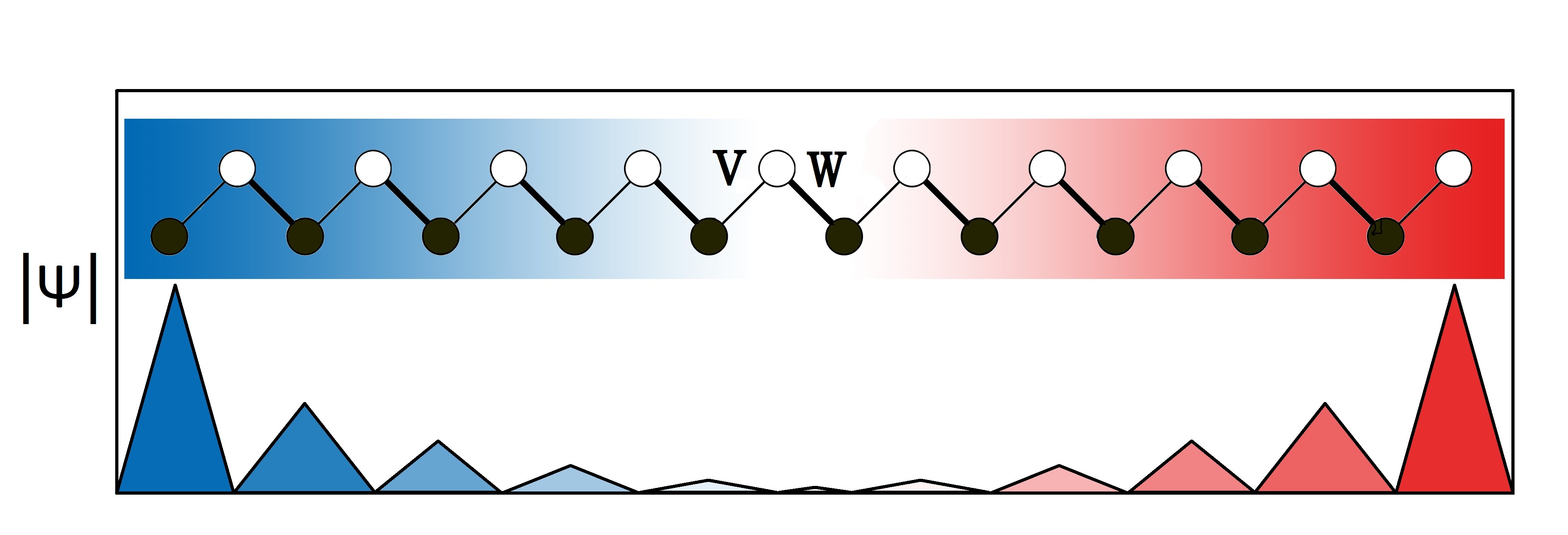
Figure 2: Amplitude $|\psi|$ of the edge-state wave function of the SSH model in Eq. (2) under an open boundary condition. Asbóth et al. (2016) Blue and red colors respectively represent the spatial distribution of the existing probability for left and right localized edge states. The total site number is set to be even, the dimerization parameter $\delta_{0}>0$, and symbols $v$ and $w$ denote hopping amplitudes $t(1-\delta_{0})$ and $t(1+\delta_{0})$, respectively. The wave-function amplitude decays exponentially into the bulk Shen (2013).

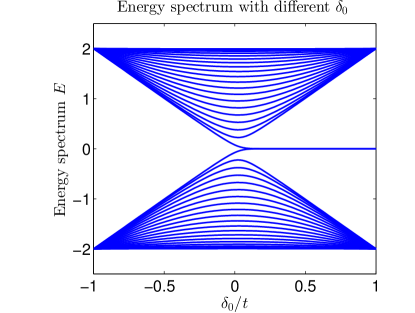
Figure 3: $\delta_{0}$ dependence of the energy spectrum of the SSH model with $t=1$ and $N=40$ under an open boundary condition. As $\delta_{0}\rightarrow 0^{+}$, two localized edge states at the ends merge into the bulk. For the limit $N\rightarrow+\infty$, the edge states are strictly at zero energy as $0<\delta\leq t$ which are protected by the chiral symmetry. Asbóth et al. (2016)

II.3 ESR of edge states

Let us consider ESR of the 1-d half-filled topological insulator phases at the low-temperature and low-frequency limit $|\omega|,T\ll|\delta_{0}|t$ on which we focus in this paper. The ESR contribution from bulk excitations is negligible in this limit since there is a large bond-alternation driven band gap $4|\delta_{0}|t$. On the other hand, spin-1/2 edge states are located at the (nearly) zero energy point in the band-gap regime. Therefore, ESR is dominated by the edge state contribution.

When the chiral symmetry is preserved and SO coupling is absent, the edge spin is precisely equivalent to a free $S=1/2$. In this case, the edge ESR spectrum is trivial, which means that it just consists of the delta function at the Zeeman energy. However, breaking of the chiral symmetry and introduction of SO couplings can bring a nontrivial change on the edge ESR spectrum. In the following, we shall analyze this effect theoretically.

In ESR, absorption of an incoming electromagnetic wave is measured under a static magnetic field. Thus we introduce the Zeeman term for the static, uniform magnetic field

$$\mathscr{H}_{Z}=-\frac{H}{2}\sum_{j=1}c^{\dagger}_{j}\left(\vec{\sigma}\cdot\vec{n}_{H}\right)c_{j},$$ (13)

where $\vec{n}_{H}$ is a unit vector representing the direction of the magnetic field, $H>0$ is its magnitude, and $\vec{\sigma}=(\sigma^{x},\sigma^{y},\sigma^{z})$.

In the paramagnetic resonance of independent electron spins, absorption occurs for the oscillating magnetic field perpendicular to the static magnetic field, which is measured in the standard Faraday configuration. Therefore, in this paper, we assume that the oscillating magnetic field is perpendicular to the static magnetic field $\vec{n}_{H}$. The frequency of the electromagnetic wave is denoted by $\omega$.

In an electron system with the SO interaction, the electric current operator contains a “SO current” that involves the spin operator. Since the electric current couples to the oscillating electric field, in the actual setting of the ESR experiment, the optical conductivity due to the SO current also contributes to the absorption of the electromagnetic wave with a spin flip. This effect is called Electron Dipole Spin Resonance (EDSR) Rashba (1960); Rashba and Efros (2003); Efros and Rashba (2006); Bolens et al. (2017). The EDSR contribution is generically larger than ESR if SO coupling is at the same order as the Zeeman splitting Shekhter et al. (2005); Maiti et al. (2016), as their relative contributions are of $(a/\lambda_{\text{C}})^{2}\approx 10^{6}$, where $a\approx 10^{-10}$m is the lattice spacing and $\lambda_{\text{C}}\approx 10^{-13}$m the Compton length of the electron Bolens et al. (2017). In general, EDSR requires a separate consideration from ESR as they involve different operators Bolens et al. (2017). Nevertheless, in the low-temperature/low-frequency regime, only the two spin states of the edge state are involved. Thus, although EDSR contributes to the absorption intensity differently from ESR, the resonance frequency is identical between the ESR and EDSR. With this in mind, we do not consider EDSR explicitly in the rest of the paper. It should be noted that, for a higher temperature or a higher frequency, the EDSR contribution to the absorption spectrum is rather different from the ESR one, as the absorption spectrum involves bulk excitations.

We now consider the ESR in the system with the Hamiltonian ${\mathscr{H}}_{0}+{\mathscr{H}}_{z}$. Within the linear response theory Kubo and Tomita (1954), the ESR spectrum is generally given by the dynamical susceptibility function in the limit of zero-momentum transfer

$$\chi^{\prime\prime}_{+-}(q=0,\omega>0) = -\text{Im}\mathscr{G}^{\text{R}}_{+-}(q=0,\omega),$$ (14)

where

$$\mathscr{G}^{\text{R}}_{+-}(0,\omega) = -i\int_{0}^{\infty}dt\sum_{r,r^{\prime}}\langle[s^{+}(r,t),s^{-}(r^{\prime},0)]\rangle e^{i\omega t}$$ (15)

$$= -i\int_{0}^{+\infty}dt\langle[S^{+}(t),S^{-}(0)]\rangle e^{i\omega t},$$

where $S^{\pm}$ means the ladder operator defined with respect to the direction $\vec{n}_{H}$ of the static field, $\langle\cdots\rangle$ denotes the quantum and ensemble average at the given temperature $T$, and

$$S^{\pm}(t)\equiv\sum_{r}\exp(i\mathscr{H}t)s^{\pm}(r)\exp(-i\mathscr{H}t)=\sum_{r}s^{\pm}(r,t),$$ (16)

where $\mathscr{H}$ is the static Hamiltonian we consider (e.g., $\mathscr{H}={\mathscr{H}}_{0}+{\mathscr{H}}_{z}$).

In the absence of SO coupling ($\phi=0$), ${\mathscr{H}}_{0}$ has the exact SU(2) spin rotation symmetry which is broken only “weakly” Oshikawa and Affleck (2002) by the Zeeman term ${\mathscr{H}}_{Z}$. As a general principle of ESR, in this case, the ESR spectrum (if any) remains paramagnetic, namely a single $\delta$-function at $\omega=H$. As we will demonstrate later in Sec. III, in the low-temperature limit, this paramagnetic ESR can be attributed to the edge states of the SSH model. Once the SO coupling is introduced ($\phi\neq 0$), the SU(2) symmetry is broken and we would expect a nontrivial ESR lineshape. However, somewhat surprisingly, (as we will show later), the ESR spectrum attributed to the edge states remains a $\delta$-function at $\omega=H$ even when $\phi\neq 0$.

Thus, in order to investigate possible nontrivial effects of the SO coupling on ESR, we further consider the NNN hoppings

$$\Delta\mathscr{H}=\sum_{j=1}\Delta tc_{j+2}^{\dagger}\exp[i\gamma\vec{n}_{\gamma}\cdot\sigma/2]c_{j}+\text{h.c.},$$ (17)

where $\Delta t$ is the NNN electron hopping amplitude. The angle $\gamma$ and $\vec{n}_{\gamma}$ are the SO turn angle and the axis for the NNN hopping, respectively.

The Hamiltonian of the system to be considered is then

$${\mathscr{H}}_{\text{ESR}} = {\mathscr{H}}_{0}+{\mathscr{H}}_{Z}+\Delta{\mathscr{H}}.$$ (18)

Once we include the NNN hoppings, the chiral symmetry is broken and the edge states are not protected to be at zero energy. Nevertheless, when the chiral symmetry breaking perturbations are weak, we may still identify “edge states” localized near the ends although they are no longer at exact zero energy even when $H=0$. Under a magnetic field $H$, contributions from these edge states dominate the ESR in the low-energy limit. Now, the ESR spectrum can be nontrivially modified by the SO couplings $\phi$ and $\gamma$. It is the main purpose of the present paper to elucidate this effect. In real materials, the NNN hoppings might be small but they are generally non-vanishing. Thus it is important to develop a theory of ESR in the presence of the NNN hoppings, especially because we can detect the NNN hoppings with ESR even when they are small.

We will treat the NNN hopping $\Delta\mathscr{H}$, which would be smaller than the NN hopping $\mathscr{H}_{0}$ in many experimental realizations, as a perturbation. This also turns out to be convenient for our theoretical analysis. We also assume that $|\phi|,|\gamma|\ll 1$ since SO couplings are weak in most of the realistic systems, and they will formulate a perturbation expansion in $\Delta t$, $\phi$, and $\gamma$.

III Edge states of ${\mathscr{H}}_{0}$ and $U(1)_{\vec{S}\cdot\vec{n}_{H}}$ symmetry

As we discussed earlier, ESR would be an ideal probe to detect the edge state of the 1D topological insulator and various perturbations. In this section, we discuss and explicitly solve the edge states of the unperturbed Hamiltonian ${\mathscr{H}}_{0}$ to demonstrate the robustness of the edge states against SO coupling. As a consequence, in the model $\mathscr{H}_{0}$ only with NN hoppings, there is no nontrivial change in the edge ESR spectrum.

Since our Hamiltonian ${\mathscr{H}}_{0}$ is bilinear in fermion operators, we can focus on single-electron states and represent them with the ket notation. For a half-infinite chain with sites $j=1,2,\ldots$, where $j=1$ corresponds to the end of the chain, we find a single-electron eigenstate $|\text{Edge},\sigma\rangle$ localized near the edge in the “topological insulator” phase $\delta_{0}>0$. Here $\sigma=\pm 1$ represents the spin component in the direction of the magnetic field. Namely,

$$\left({\mathscr{H}}_{0}+{\mathscr{H}}_{Z}\right)|\text{Edge,}\sigma\rangle = E^{(0)}_{\sigma}|\text{Edge,}\sigma\rangle$$ (19)

$$\vec{S}\cdot\vec{n}_{H}|\text{Edge,}\sigma\rangle = \frac{\sigma}{2}|\text{Edge,}\sigma\rangle,$$ (20)

with the energy eigenvalues $E^{(0)}_{\sigma}=-\sigma H/2$ and $\vec{S}$ is the total spin of the system. The wave function of the edge states is exactly calculated as

$$\langle j,\sigma|\text{Edge,}\sigma^{\prime}\rangle=\begin{cases}\frac{\delta_{\sigma\sigma^{\prime}}}{\sqrt{\mathscr{N}}}\left(-\frac{1-\delta_{0}}{1+\delta_{0}}\right)^{(j-1)/2}&\mbox{ ($j\in 2\mathbb{N}_{0}+1$ )},\\ 0&(\mbox{otherwise}),\end{cases}$$ (21)

where $2\mathbb{N}_{0}$ is the set of non-negative even integers, and $\mathscr{N}$ is the normalization constant. The energy eigenvalue of the edge state for ${\mathscr{H}}_{0}$ is, independently of the spin component, exactly zero, reflecting its topological nature.

It is also remarkable that the edge state wavefunction is independent of $\phi$ and $\vec{n}$. This is a consequence of a canonical “gauge transformation” Gangadharaiah et al. (2008)

$$\tilde{c}_{2k+1} =c_{2k+1},$$ (22)

$$\tilde{c}_{2k} =\exp{\left(i\phi\vec{n}\cdot{\vec{\sigma}}/2\right)}c_{2k},$$

which eliminates the SO coupling from ${\mathscr{H}}_{0}$. In this sense, ${\mathscr{H}}_{0}$ still has a hidden SU(2) symmetry Kaplan (1983); Shekhtman et al. (1992) even though the SO coupling breaks the apparent spin SU(2) symmetry. However, since the gauge transformation involves the local rotation of spins, the uniform magnetic field ${\mathscr{H}}_{Z}$ gives rise to a staggered field after the gauge transformation. This staggered field completely breaks the SU(2) symmetry. This is similar to the situation in a spin chain with a staggered Dzyaloshinskii-Moriya interaction Oshikawa and Affleck (1999). Thus, following the general principle of ESR, we would expect a nontrivial ESR spectrum in the presence of the staggered SO coupling as in ${\mathscr{H}}_{0}$.

Nevertheless, somewhat unexpectedly, we find that the edge ESR spectrum for the model ${\mathscr{H}}_{0}$ remains the $\delta$-function $\delta(\omega-H)$, as if there is no anisotropy at all. This is due to the fact that the edge-state wavefunction Eq. (21) is non-vanishing only on the even sites. Since the gauge transformation can be defined so that it only acts on the even sites where the edge-state wavefunction Eq. (21) vanishes, the edge state is completely insensitive to the SO coupling. Therefore, the spectral shape of the edge ESR remains unchanged by the staggered SO coupling. In addition, since the edge wave functions are eigenstates of the total spin component along $\vec{n}_{H}$ according to Eq. (20), the edge states have $U(1)_{\vec{S}\cdot\vec{n}_{H}}$ symmetry generated by $\vec{S}\cdot\vec{n}_{H}$.

In fact, the robustness of the edge ESR spectrum is valid for a wider class of models. The edge ESR only probes a transition between two states with opposite polarization of the spin, which form a Kramers pair in the absence of the magnetic field. Thus, at zero magnetic field, the time-reversal invariance of the model requires these two states to be exactly degenerate. For a finite magnetic field, if the system still has $U(1)_{\vec{S}\cdot\vec{n}_{H}}$ symmetry of rotation about the magnetic field axis, the two states can be labelled by the eigenvalues of $S^{z}=\pm 1/2$, and their energy splitting is exactly

$$\omega_{\text{ESR}}=H.$$ (23)

Thus, as far as the edge ESR involving only the Kramers pair is concerned, the $U(1)_{\vec{S}\cdot\vec{n}_{H}}$ symmetry is sufficient to protect the $\delta$-function peak at $\omega=H$. We note that, more generally, when more than two states contribute to ESR, these symmetries are not sufficient to protect the single-peak ESR spectrum, as there can be transitions between states not related by time reversal. In fact, this would be the case for the absorption due to bulk excitations which we do not discuss in this paper.

IV Perturbation theory of the edge ESR frequency shift

As we have shown in the previous Section, even in the presence of SO coupling, there is no frequency shift for edge ESR in the NN hopping model ${\mathscr{H}}_{0}$. This is a consequence of the chiral symmetry, which stems from the bipartite nature of the NN hopping model.

As we will discuss below, the introduction of NNN hoppings breaks the chiral symmetry and generally causes a nontrivial frequency shift of the edge ESR. In this Section, we develop a perturbation theory of ESR for the edge states, first by regarding ${\mathscr{H}}_{0}+{\mathscr{H}}_{Z}$ as the unperturbed Hamiltonian and $\Delta\mathscr{H}$ as a perturbation.

In the presence of the perturbation with SO couplings, the eigenstate of the Hamiltonian is generally no longer an eigenstate of the spin component $\vec{S}\cdot\vec{n}_{H}$ as in Eq. (20). Nevertheless, as long as the perturbation theory is valid, two edge states can still be identified by using spin $\sigma=+$ and $-$. Namely, for the full Hamiltonian (18), we can define the edge state labeled by $\sigma=\pm$ as the state adiabatically connected to $|{\rm Edge},\pm\rangle$ as $\Delta{\mathscr{H}}\to 0$.

Here let us introduce new symbols $E_{+(-)}$ and $E_{+(-)}^{(n)}$ as the energy eigenvalue of the almost spin up (down) edge state in Eq. (18) and its $n$-th order correction in the perturbation theory, respectively. With these symbols, the ESR frequency is given by

$$\omega_{\text{ESR}}=E_{-}-E_{+}=H+\Delta\omega,$$ (24)

where the ESR trivial peak position is given by $E^{(0)}_{-}-E^{(0)}_{+}=H$. The ESR frequency shift $\Delta\omega$, driven by the perturbation $\Delta{\mathscr{H}}$, is expanded in the perturbation theory as

$${\Delta\omega}={\Delta\omega}^{(1)}+{\Delta\omega}^{(2)}+\ldots,$$ (25)

where the $n$-th order term is

$${\Delta\omega}^{(n)}=E^{(n)}_{-}-E^{(n)}_{+},$$ (26)

for $n\in\mathbb{N}$. In the following parts, we perturbatively solve the single-electron problem to compute the eigen-energy difference of two edge states $E_{+}$ and $E_{-}$.

IV.1 First order in $\Delta t$

The NNN hopping $\Delta\mathscr{H}$ breaks the chiral symmetry, and thus it can change the edge ESR spectrum. In fact, the energy of the edge states is already shifted in the first order of $\Delta\mathscr{H}$. However, the energy shift is the same for the two edge states with different spin polarizations. This is a consequence of the time-reversal (TR) symmetry of the SO coupling, as demonstrated below:

$$E_{\sigma}^{(1)} = \langle\text{Edge,}\sigma|\Delta\mathscr{H}|\text{Edge,}\sigma\rangle$$ (27)

$$= \langle\Theta\left(\text{Edge,}-\sigma\right)|\Theta\Delta\mathscr{H}\Theta^{-1}|\Theta\left(\text{Edge,}-\sigma\right)\rangle$$

$$= E_{-\sigma}^{(1)}$$

$$= -2\Delta t\frac{1-\delta_{0}}{1+\delta_{0}}\cos\left(\frac{\gamma}{2}\right)$$

where $\Theta$ is the TR operator and $\Theta\Delta\mathscr{H}\Theta^{-1}=\Delta\mathscr{H}$ is used. Therefore, the edge ESR spectrum remains unchanged in the first order of $\Delta t$ as the frequency shift vanishes in this order:

$${\Delta\omega}^{(1)}=E^{(1)}_{-}-E^{(1)}_{+}=0.$$ (28)

IV.2 Second order in $\Delta t$

We can formally write down the second-order perturbation correction

$$E_{\sigma}^{(2)}=\langle\text{Edge,}\sigma|\Delta\mathscr{H}\!\!\cdot\!(E^{(0)}_{\sigma}-\mathscr{H}_{0})^{-1}\!\!\cdot\!\!\mathscr{P}_{\sigma}\!\cdot\!\Delta\mathscr{H}|\text{Edge,}\sigma\rangle$$

where the projection operator $\mathscr{P}_{\sigma}\equiv 1-|\text{Edge,}\sigma\rangle\langle\text{Edge,}\sigma|$. It is rather difficult to evaluate this formula directly, since the intermediate states in the perturbation term include the bulk eigenstates of $\mathscr{H}_{0}$ in which the hidden symmetry is generally broken. Assuming that $|\phi|,|\gamma|\ll 1$ (i.e., the SO coupling is sufficiently small), we can develop a perturbative expansion in $\phi$ and $\gamma$ in addition to $\Delta t$. In this framework, we expand $E_{\sigma}$ as a Taylor series of $\phi$, $\gamma$ and $\Delta t$. The quantity of interest is the energy splitting $E_{-}-E_{+}$, since it corresponds to the ESR frequency.

The edge state energy splitting in the second order in $\Delta t$, and up to the second order in $\phi$, $\gamma$ is required to take the form

$$E^{(2)}_{\sigma}-E^{(2)}_{-\sigma} \approx \frac{1}{2}\sigma H\Delta t^{2}\left\{a(\vec{n}_{\gamma}\times\vec{n}_{H})^{2}\gamma^{2}+b(\vec{n}\times\vec{n}_{H})^{2}\phi^{2}\right.$$ (29)

$$\left.+c(\vec{n}\times\vec{n}_{H})\cdot(\vec{n}_{\gamma}\times\vec{n}_{H})\phi\gamma\right\},$$

based on the following symmetry considerations, and $a$, $b$ and $c$ are constants to be determined.

First of all, $(E_{\sigma}-E_{-\sigma})$ will not change under

$$(H,\vec{n}_{H},\sigma)\to(-H,-\vec{n}_{H},-\sigma),$$ (30)

because this corresponds to a trivial redefinition of coordinate system. Therefore, we attach the factor $\sigma H$ in the r.h.s. of Eq. (29).

Next we notice that $\phi$ always appears with $\vec{n}$, and $\gamma$ with $\vec{n}_{\gamma}$, which leads to further constraints as we will see below. Let us consider the limiting case $\phi=0$ with nonzero $\gamma$. The splitting can only depend on the relative angle between $\vec{n}_{\gamma}$ and $\vec{n}_{H}$. Furthermore, if $\vec{n}_{\gamma}\parallel\vec{n}_{H}$, the hidden symmetry of the edge state implies that the energy splitting is exactly given by the Zeeman energy and there is no perturbative correction. Thus, for $\phi=0$, the energy splitting can only depend on $(\vec{n}_{\gamma}\times\vec{n}_{H})^{2}\gamma^{2}$ up to $O(\gamma^{2})$ since the energy split is a scalar and it must be written in terms of inner and vector products of $\vec{n}_{H}$, $\vec{n}$ and $\vec{n}_{\gamma}$. Then, similarly, if $\gamma=0$ with nonzero $\phi$, the energy splitting can only depend on $(\vec{n}\times\vec{n}_{H})^{2}\phi^{2}$. Finally, the $O(\phi\gamma)$ term should be linear in $\vec{n}$ and $\vec{n}_{\gamma}$, and it vanishes when $\vec{n}\parallel\vec{n}_{\gamma}\parallel\vec{n}_{H}$ because of the $U(1)_{\vec{S}\cdot\vec{n}}$ symmetry. These requirements uniquely determine the form of $(\vec{n}\times\vec{n}_{H})\cdot(\vec{n}_{\gamma}\times\vec{n}_{H})$. Thus, the symmetries reduce the possible forms of the second-order corrections to Eq. (29) with only the three parameters $a$, $b$, and $c$.

To obtain these parameters, we note that the expansion in $\phi$ and $\gamma$ introduced above can be naturally done by regarding the SSH model without SO coupling

$$\tilde{\mathscr{H}}_{0} = -\sum_{j=1}^{+\infty}\left\{t\left[1+(-1)^{j}\delta_{0}\right]c_{j+1}^{\dagger}c_{j}+\text{h.c.}\right\}$$ (31)

$$-H\sum_{j=1}c^{\dagger}_{j}\left(\vec{\sigma}\cdot\vec{n}_{H}\right)c_{j}/2$$

as the unperturbed Hamiltonian, and

$$\mathscr{H}_{\text{pert}}=\Delta\mathscr{H}_{0}+\Delta\mathscr{H},$$ (32)

as the perturbation, where

$$\Delta\mathscr{H}_{0} \equiv -\sum_{j=1}^{+\infty}\left\{t\left[1+(-1)^{j}\delta_{0}\right]c_{j+1}^{\dagger}\right.$$ (33)

$$\left.\left\{\exp\left[(-1)^{j}i\phi\vec{n}\cdot\vec{\sigma}/2\right]-1\right\}c_{j}+\text{h.c.}\right\}$$

and $\Delta\mathscr{H}$ as defined in Eq. (17).

As the result of the perturbation calculation given in the Appendix, we find that the second-order term of frequency shift is non-positive given in the form

$$\Delta\omega^{{(2)}} = -\frac{H}{2}\sum_{m_{3},j_{3}}(\vec{M}+\vec{N})^{\dagger}\cdot(\vec{M}+\vec{N})\leq 0,$$ (34)

where

$$\vec{M} \equiv \sum_{m_{2},j_{2}}\!\!\frac{\langle m_{3},j_{3}|\Delta\mathscr{H}^{\prime}_{0}|m_{2},j_{2}\rangle\langle m_{2},j_{2}|\Delta\mathscr{H}^{\prime\prime}|\text{Edge}\rangle}{m_{2}E_{j_{2}}E_{j_{3}}}$$

$$(\vec{n}\times\vec{n}_{H})\phi$$

$$\vec{N} \equiv \frac{\langle m_{3},j_{3}|\Delta\mathscr{H}^{\prime}|\text{Edge}\rangle}{E_{j_{3}}}(\vec{n}_{\gamma}\times\vec{n}_{H})\gamma.$$ (35)

Here $|m,j\rangle$’s are single-particle (bulk) energy eigenstates of $\tilde{\mathscr{H}}_{0}$ in Eq. (31) where $m=\pm$ labels the positive or negative energy sector (i.e., band indices) and $j$ labels other possible quantum numbers, which is not the wave vector since we have the open-ended boundary condition. The energy $\pm E_{j}$ stands for the energy eigenvalue of $|\pm,j\rangle$. The perturbation terms $\Delta\mathscr{H}^{\prime}$, $\Delta\mathscr{H}^{\prime\prime}$, and $\Delta\mathscr{H}^{\prime}_{0}$ are defined as

$$\Delta\mathscr{H}^{\prime}\equiv\sum_{j=1}\Delta tc^{\dagger}_{j+2}c_{j}-\text{h.c.},$$ (36)

$$\Delta\mathscr{H}^{\prime\prime}\equiv\sum_{j=1}\Delta tc^{\dagger}_{j+2}c_{j}+\text{h.c.},$$ (37)

$$\Delta\mathscr{H}^{\prime}_{0}\equiv-\sum_{j=1}^{+\infty}\left\{t\left[1+(-1)^{j}\delta_{0}\right]c_{j+1}^{\dagger}c_{j}-\text{h.c.}\right\}.$$ (38)

We note that Eqs. (36) and (38) are anti-Hermitian.

After putting the definitions of $\vec{M}$ and $\vec{N}$ into Eq. (34), we find the result consistent with the general form Eq. (29) required by symmetries. The parameters are then identified as

$$a = b=\left[\frac{\Delta t}{t(1+\delta_{0})}\right]^{2},\quad c=-2\left[\frac{\Delta t}{t(1+\delta_{0})}\right]^{2}.$$

The detailed derivation of $a$, $b$ and $c$ is given in Appendix. The final result can be given in a compact form as

$${\Delta\omega}^{(2)}=-\frac{H}{2}\left|\frac{\Delta t}{t(1+\delta_{0})}(\phi\vec{n}\times\vec{n}_{H}-\gamma\vec{n}_{\gamma}\times\vec{n}_{H})\right|^{2},$$ (39)

which is non-positive. Since the first-order correction vanishes as we have already seen, the second-order term Eq. (39) gives the leading term for the frequency shift of the edge ESR. It also implies that, although $\gamma$ is the SO-coupling turn angle for the NNN hopping terms, it is equally important in $\Delta\omega$ as the NN SO coupling turn angle $\phi$ even if the NNN hopping itself is small ($\Delta t\ll t$).

One of the most remarkable features of our result is that, the shift (up to the second order in the perturbation) vanishes when $\phi\vec{n}\times\vec{n}_{H}=\gamma\vec{n}_{\gamma}\times\vec{n}_{H}$. This corresponds to the zeros of curves in Fig. 4 where the direction of the magnetic field is in the plane spanned by $\vec{n}=\hat{y}$ and $\vec{n}_{\gamma}=-\hat{z}$, and $\theta$ is the angle between $\vec{n}_{H}$ and $\hat{y}$ in the $\hat{y}$-$\hat{z}$ plane, as shown in Fig. 5. Therefore, we predict two directions of the magnetic field for which the ESR shift vanishes, when the magnetic field direction $\vec{n}_{H}$ sweeps the plane spanned by $\vec{n}$ and $\vec{n}_{\gamma}$.

V Non-perturbative calculation of the edge ESR spectrum

Here, in order to see the validity of our perturbation theory in the preceding section, let us re-compute the edge ESR frequency with a more direct numerical method. As already mentioned, when the magnetic field $H$ (and thus the ESR frequency $\omega$) is much smaller compared to the bulk excitation gap $4t|\delta_{0}|$, we may ignore the effects of the bulk excitations in the ESR spectrum. Then the edge ESR spectrum is of the $\delta$-function form

$$\chi^{\prime\prime}_{+-\text{edge}}(q=0,\omega) \propto \delta\left[\omega-(E_{-}-E_{+})\right],$$ (40)

where $E_{+(-)}$ is the energy eigenvalue of the “almost” spin-up (spin-down) edge state. These energies can be accurately computed by numerical diagonalization of a finite (but long) size full Hamiltonian with an open boundary condition. Then we obtain the spectrum peak shift ${\Delta\omega}\equiv E_{-}-E_{+}-H$ from the numerical results of $E_{\pm}$. In the present work, we calculated $E_{\pm}$ using a finite open chain of 100 sites.

In Fig. 4, we compare the numerical results of the peak shift with the analytical perturbation theory of $\Delta\omega_{\text{ESR}}^{(2)}$ in Eq. (39) when the magnetic field is in the plane spanned by $\vec{n}$ and $\vec{n}_{\gamma}$. The figure clearly shows that our perturbation theory agrees with the numerical results quite well.

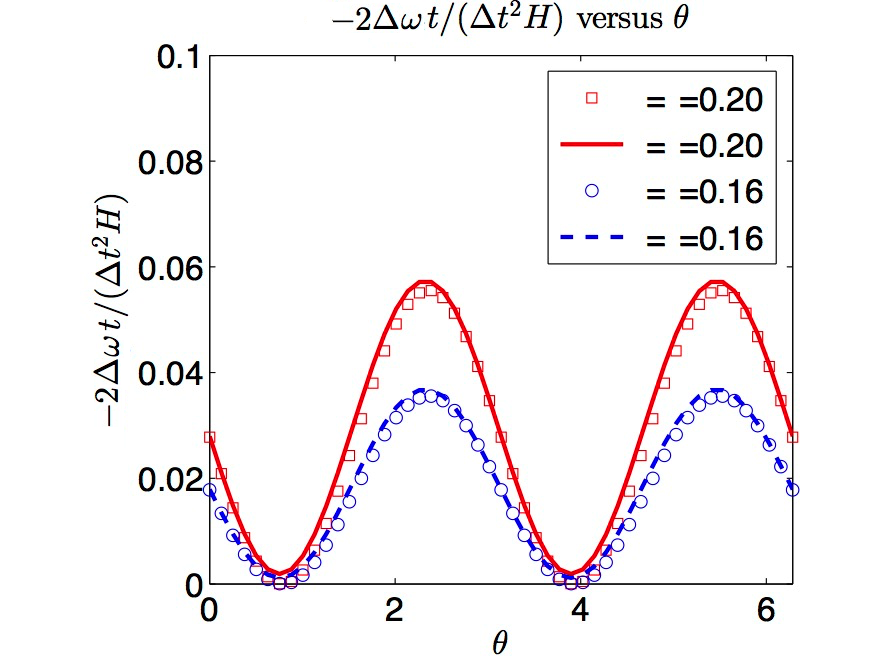
Figure 4: Angle $\theta$ dependence of the ESR frequency shift $\Delta\omega$. We set the parameters $t=1.0$, $\Delta t=\delta_{0}=0.2$, and $H=0.05$. Red and blue curves are obtained by the second-order perturbation calculation in Sec. IV.2. Square and circle points are the results of direct numerical diagonalization for a system (of 100 sites) with an open boundary condition. The definition of angle $\theta$ is indicated in Fig. 5. The zeros of $\Delta\omega$ occur at $\phi\vec{n}\times\vec{n}_{H}=\gamma\vec{n}_{\gamma}\times\vec{n}_{H}$.

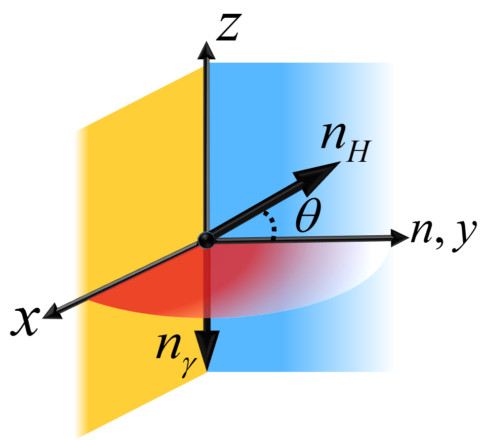
Figure 5: Geometric relation among some vectors in Fig. 4, where the direction of magnetic field is in the plane spanned by $\vec{n}=\hat{y}$ and $\vec{n}_{\gamma}=-\hat{z}$. The parameter $\theta$ is defined as the angle between $\vec{n}_{H}$ and $\hat{y}$ in the $\hat{y}$-$\hat{z}$ plane.

VI Conclusions and Discussion

We have analyzed ESR of edge states in a generalized SSH model with staggered SO couplings and with an open end. In this paper, we assume that the energy scales of the magnetic field, the frequency, and the temperature are sufficiently small compared to the bulk gap. Then the ESR spectrum only consists of a single $\delta$-function spectrum corresponding to the transition between two spin states at the edge, but is expected to show a nontrivial frequency shift in general as the SO coupling breaks the SU(2) symmetry strongly under the applied magnetic field. Nevertheless, there is no ESR frequency shift in the model with only NN hoppings, thanks to its chiral symmetry.

The chiral symmetry is broken by NNN hoppings, which should be generally present in any realistic materials even if they are small. This NNN hoppings, together with the SO coupling, can induce a nontrivial frequency shift on the edge ESR. Thus we have developed a perturbation theory of the frequency shift, regarding the NNN hoppings and the SO couplings as perturbations. Our main result, the ESR frequency shift up to second order in the perturbation theory, is found in Eq. (29). It is non-positive in this order. (The resonance field shift for a fixed frequency, which is usually measured in experiments, is always positive.) In the presence of the NNN hoppings, the SO couplings in the NN hoppings, which did not cause a frequency shift by themselves, also contribute to the frequency shift. We find an interesting dependence of the ESR frequency shift on the direction of the static magnetic field, relative to the SO couplings on the NN and the NNN hoppings. In particular, the ESR frequency shift is predicted to vanish when the static magnetic field points to a certain direction on the plane spanned by the two SO coupling axes (see Fig. 4). Furthermore, we performed a direct estimate of the ESR frequency shift by a numerical calculation of the edge state spectrum, without relying on the perturbation theory. The result agrees very well with the perturbation theory, establishing its validity.

Our results indicate that, the chiral symmetry breaking by the NNN hoppings in the “SSH”-type topological insulators in one dimension may be detected by ESR, in the presence of the SO couplings. If the NNN hoppings are small, which would be the case in many realistic materials, it might be difficult to detect their effects with other experimental techniques. ESR has been successful in detecting even very small magnetic anisotropies, thanks to its high sensitivity and accuracy. We hope that the present work will pave the way for a new application of ESR in detecting (small) chiral symmetry breaking.

While we do not discuss any particular material in this paper, let us discuss here the prospect of experimentally observing the effects we predict. The maximal frequency shift is given by the order of

$$H\left(\frac{\Delta t}{t}\max{\{\phi,\gamma\}}\right)^{2}.$$ (41)

The ratio of NNN to NN hoppings, $\Delta t/t$, of course strongly depends on each material. It is even possible that $|\Delta t|/t\gg 1$, in which case the system may be regarded as two chains coupled weakly by zigzag hopping. It should be however noted that our theory is valid only when $|\Delta t|/t$ is sufficiently small. We still expect that our theory works reasonably well for $(\Delta t/t)^{2}\sim 0.1$. In carbon-based systems, such as polyacetylene, the SO interaction is known to be weak. For example, even with the enhanced SO interaction due to a curvature Huertas-Hernando et al. (2006), $\phi,\gamma$ is of order of $10^{-5}$. This would give an ESR shift that is too small to be observed in experiments. However, the SO interaction is stronger in heavier atoms. In fact, even in carbon-based systems, the SO interaction can be significantly enhanced by heavy adatoms. For example, placing Pb as adatoms can enhance $\phi,\gamma$ up to $0.1$ or more in graphene Brey (2015). This would give the edge ESR shift corresponding to the $g$-shift up to the order of $10^{-3}$ (1,000 ppm), which should be observable. In particular, even if the absolute value of the shift is difficult to be determined, the angular dependence of the ESR shift would be more evident in experiments. Furthermore, it is known that an SO interaction generally becomes larger when the electron system we consider is located in the vicinity of an interface between two bulk systems or is under a strong, static electric field Nitta et al. (1997); Caviglia et al. (2010); Soumyanarayanan et al. (2016). Therefore, if we set up an SSH chain system under such an environment, it would become easier to detect an ESR frequency shift due to a strong SO coupling.

Throughout this paper, we have taken the NN SO coupling in the model Eq. (1) to be staggered. However, there are other possibilities. In particular, in a translationally symmetric system, the NN SO coupling is uniform. Although the only difference is the signs in the Hamiltonian, ESR spectra should be significantly different between these two cases. This is clear if we consider the limit of the zero NNN hopping. In the staggered SO coupling case, there is no ESR frequency shift. This is because the NN SO coupling can be gauged out by the canonical transformation Eq. (22), without changing the odd site amplitude and thus leaving the SSH edge state wavefunction Eq. (21) unchanged. On the other hand, in the uniform SO coupling case, gauging out the NN SO coupling affects any wavefunction including the SSH edge state wavefunction, resulting in the change of the ESR spectrum. A similar difference has been recognized between the ESR spectum in the presence of a staggered DM interaction Oshikawa and Affleck (1999) and that with a uniform DM interaction along the chain Gangadharaiah et al. (2008). The analysis of the edge ESR spectrum in the presence of a uniform SO coupling is left for future studies.

*

Appendix A Perturbation theory for the frequency shift $\Delta\omega$

Here we explain how to determine the parameters $a$, $b$ and $c$ in the general form of Eq. (29), based on a perturbation theory. As we have discussed earlier, in order to expand the edge-state energy eigenstates with respect to the SO coupling parameters $\phi$ and $\gamma$, which are assumed to be small, we regard $\tilde{{\mathscr{H}}}_{0}$ of Eq. (31) as the unperturbed part, and $\tilde{{\mathscr{H}}}_{\text{pert}}$ of Eq. (32) as the perturbation. Moreover, we have already shown in Sections III and IV.1 that the ESR shift vanishes exactly up to $O(\Delta t)$. Therefore, the leading terms with coefficients $a$, $b$ and $c$ stem from the second-order perturbation proportional to $\Delta t^{2}$. Below, we will determine three parameters $a$, $b$ and $c$ from the perturbative expansion of $\tilde{{\mathscr{H}}}_{\text{pert}}$.

A.1 Second order in ${\mathscr{H}}_{\text{pert}}$

The shift of the edge energy eigenvalue in the second order of ${\mathscr{H}}_{\text{pert}}$ is given by

$$E^{[2]}_{\sigma}\!\! = \!\!\!\!\!\sum_{m=\pm,j,\tilde{\sigma}=\pm}\!\!\!\!\!\!\!\!\frac{\langle\text{Edge,}\sigma|\mathscr{H}_{\text{pert}}|m,j,\tilde{\sigma}\rangle\!\langle m,j,\tilde{\sigma}|\mathscr{H}_{\text{pert}}|\text{Edge,}\sigma\rangle}{-\sigma\frac{H}{2}-E_{m,j,\tilde{\sigma}}}$$ (42)

$$\approx \sum_{m=\pm,j}\frac{\langle\text{Edge}|(\Delta\mathscr{H}^{\prime})^{\dagger}|m,j\rangle\langle m,j|\Delta\mathscr{H}^{\prime}|\text{Edge}\rangle}{E^{2}_{j}}\sigma H$$

$$\cdot|n_{\gamma}\times n_{H}|^{2}{\gamma^{2}}/{4},$$

where the bulk single-particle eigen-energy $E_{m,j,\tilde{\sigma}}$ is given by

$$E_{m,j,\tilde{\sigma}} \equiv mE_{j}-\tilde{\sigma}{H}/{2}$$ (43)

with $mE_{j}$ the energy eigenvalue of spinless single-particle eigenstates $|m,j\rangle$, and we have used the facts that in the unperturbed sector, the orbital and spin parts of single-particle eigenstates can be decomposed, e.g. $|m,j,\sigma\rangle=|m,j\rangle|\sigma\rangle$ since $\tilde{\mathscr{H}}_{0}$ commutes with the spin operator of each site. Here we define $E^{[n]}_{\sigma}$ as the energy eigenvalue of the edge state with spin $\sigma$ in the $n$-th order of perturbation in ${\mathscr{H}}_{\text{pert}}$. This is to be distinguished from $E^{(n)}_{\sigma}$ introduced in Eq. (26), where $n$ refers to the order in $\Delta t$. In the second line of Eq. (42), we assume $|E_{m,j,\tilde{\sigma}}|\gg H$ and perform the Taylor expansion of $E^{[2]}_{\sigma}$ with respect to $H$. The matrix $\langle m,j|\Delta\mathscr{H}^{\prime}|\text{Edge}\rangle$ can be calculated by using the anti-Hermitian operator $\Delta\mathscr{H}^{\prime}$ of Eq. (36). From Eq. (42), the ESR frequency shift driven by $E^{(2)}_{\sigma}$ is expressed as

$$E_{-}^{[2]}-E_{+}^{[2]}=-|n_{\gamma}\times n_{H}|^{2}{\gamma^{2}}/{2}$$

$$\!\!\cdot\sum_{m=\pm,j}\!\!\!\frac{\langle\text{Edge}|(\Delta\mathscr{H}^{\prime})^{\dagger}|m,j\rangle\langle m,j|\Delta\mathscr{H}^{\prime}|\text{Edge}\rangle}{E^{2}_{j}}H.$$ (44)

This indeed corresponds to the parameter $a$. To obtain $b$ and $c$, we should proceed to higher orders of ${\mathscr{H}}_{\text{pert}}$.

A.2 Third order in ${\mathscr{H}}_{\text{pert}}$

In the third order perturbation theory within $\Delta t^{2}$, the energy correction takes the form as

$$E_{\sigma}^{[3]}=\sum_{m,j,\tilde{\sigma}}\frac{\langle\text{Edge,}\sigma|\mathscr{H}_{\text{pert}}|m_{3},j_{3},\tilde{\sigma}_{3}\rangle\langle m_{3},j_{3},\tilde{\sigma}_{3}|\mathscr{H}_{\text{pert}}|m_{2},j_{2},\tilde{\sigma}_{2}\rangle\langle m_{2},j_{2},\tilde{\sigma}_{2}|\mathscr{H}_{\text{pert}}|\text{Edge,}\sigma\rangle}{\left[-(\sigma-\tilde{\sigma}_{2})\frac{H}{2}-m_{2}E_{j_{2}}\right]\left[-(\sigma-\tilde{\sigma}_{3})\frac{H}{2}-m_{3}E_{j_{3}}\right]}$$ (45)

$$+\langle\text{Edge,}\sigma|\mathscr{H}_{\text{pert}}|\text{Edge,}\sigma\rangle\frac{|\langle\text{Edge,}\sigma|\mathscr{H}_{\text{pert}}|m_{3},j_{3},\tilde{\sigma}_{3}\rangle|^{2}}{\left[-(\sigma-\tilde{\sigma}_{3})\frac{H}{2}-m_{3}E_{j_{3}}\right]^{2}}$$

$$\approx \sum_{m,j}\text{Re}\left[\frac{\langle\text{Edge}|\Delta\mathscr{H}^{\prime\prime}|m_{3},j_{3}\rangle\langle m_{3},j_{3}|\Delta\mathscr{H}^{\prime}_{0}|m_{2},j_{2}\rangle\langle m_{2},j_{2}|\Delta\mathscr{H}^{\prime}|\text{Edge}\rangle}{m_{3}E^{2}_{j_{2}}E_{j_{3}}}\sigma H\right]\cdot(\vec{n}\times\vec{n}_{H})\cdot(\vec{n}_{\gamma}\times\vec{n}_{H})\frac{\phi\gamma}{2},$$

where $\Delta\mathscr{H}^{\prime\prime}$ is defined by Eq. (37).

Therefore,

$$E_{-}^{[3]}-E_{+}^{[3]}$$

$$= \sum_{m,j}\!-\!\text{Re}\!\!\left[\frac{\langle\text{Edge}|\Delta\mathscr{H}^{\prime\prime}|m_{3},j_{3}\rangle\langle m_{3},j_{3}|(\Delta\mathscr{H}^{\prime}_{0})^{\dagger}|m_{2},j_{2}\rangle}{m_{3}E^{2}_{j_{2}}E_{j_{3}}}\right.$$

$$\left.\cdot\langle m_{2},j_{2}|\Delta\mathscr{H}^{\prime}|\text{Edge}\rangle H\right](\vec{n}\times\vec{n}_{H})\cdot(\vec{n}_{\gamma}\times\vec{n}_{H})\phi\gamma.$$

We see that this correction term corresponds to the parameter $c$ in Eq. (29).

A.3 Fourth order in ${\mathscr{H}}_{\text{pert}}$

In order to derive the leading term of the parameter $b$, we have to calculate the fourth-order term. For convenience of the fourth-order calculation, we introduce the abbreviated notation of the matrix elements:

$$A^{qr} \equiv \langle m_{r},j_{r},\tilde{\sigma}_{r}|A|m_{q},j_{q},\tilde{\sigma}_{q}\rangle,$$ (47)

$$E_{\text{E}q} \equiv E^{[0]}_{\sigma}-E_{m_{q},j_{q},\tilde{\sigma}_{q}}$$ (48)

for any operator $A$, and denote the zeroth order edge state by “E”. In this notation, the fourth order edge-energy correction up till $(\Delta t\phi)^{2}$-order is given by

$$E_{\sigma}^{[4]}=\sum_{m,j,\tilde{\sigma}}\frac{\Delta\mathscr{H}^{\text{E}4}\mathscr{H}_{\text{pert}}^{4,3}\mathscr{H}_{\text{pert}}^{3,2}\Delta\mathscr{H}^{2\text{E}}}{E_{\text{E}2}E_{\text{E}3}E_{\text{E}4}}-E_{\sigma}^{[2]}\frac{\left(\Delta\mathscr{H}^{\text{E}4}\right)^{2}}{(E_{\text{E}4})^{2}}-2\Delta\mathscr{H}^{\text{EE}}\frac{\Delta\mathscr{H}^{\text{E}4}\mathscr{H}_{\text{pert}}^{43}\Delta\mathscr{H}^{3\text{E}}}{E_{\text{E}3}^{2}E_{\text{E}4}}+\left(\Delta\mathscr{H}^{\text{EE}}\right)^{2}\frac{\left(\Delta\mathscr{H}^{\text{E}4}\right)^{2}}{(E_{\text{E}3})^{3}}$$ (49)

$$\approx \sum_{m,j,}\frac{\langle\text{Edge}|\Delta\mathscr{H}^{\prime\prime}|m_{2},j_{2}\rangle\langle m_{2},j_{2}|(\Delta\mathscr{H}^{\prime}_{0})^{\dagger}|m_{3},j_{3}\rangle\langle m_{3},j_{3}|\Delta\mathscr{H}^{\prime}_{0}|m_{4},j_{4}\rangle\langle m_{4},j_{4}|\Delta\mathscr{H}^{\prime\prime}|\text{Edge}\rangle}{m_{2}m_{4}E_{j_{2}}E^{2}_{j_{3}}E_{j_{4}}}{\sigma H}|\vec{n}\times\vec{n}_{H}|^{2}\frac{\phi^{2}}{4}.$$

Then we can arrive at

$$E_{-}^{[4]}-E_{+}^{[4]}$$ (50)

$$\approx \!-\!\!\sum_{m,j,}\!\!\frac{\langle\text{Edge}|\Delta\mathscr{H}^{\prime\prime}|m_{2},j_{2}\rangle\langle m_{2},j_{2}|(\Delta\mathscr{H}^{\prime}_{0})^{\dagger}|m_{3},j_{3}\rangle\langle m_{3},j_{3}|\Delta\mathscr{H}^{\prime}_{0}|m_{4},j_{4}\rangle\langle m_{4},j_{4}|\Delta\mathscr{H}^{\prime\prime}|\text{Edge}\rangle}{m_{2}m_{4}E_{j_{2}}E^{2}_{j_{3}}E_{j_{4}}}{H}|\vec{n}\times\vec{n}_{H}|^{2}\frac{\phi^{2}}{2}.$$

This correspond to the term coefficiented by the parameter $b$ in Eq. (29).

A.4 Summation over the perturbation orders

Through some algebra, we find that terms of the fifth and higher orders in ${\mathscr{H}}_{\text{pert}}$ do not contribute to the order of $\mathscr{O}\left(\Delta t^{2}\phi^{2}\right)$. Summing up Eqs. (28), (A.1), (A.2), and (50), we arrive at the energy shift of the energy difference between down- and up-spin edge states in an elegant form as in Eq. (34).

References

- Hasan and Kane (2010) M. Z. Hasan and C. L. Kane, Rev. Mod. Phys. 82, 3045 (2010).
- Qi and Zhang (2011) X.-L. Qi and S.-C. Zhang, Rev. Mod. Phys. 83, 1057 (2011).
- Bernevig and Hughes (2013) B. A. Bernevig and T. L. . X. Hughes, Topological insulators and topological superconductors (Princeton University Press, 2013).
- Shen (2013) S.-Q. Shen, Topological Insulators: Dirac Equation in Condensed Matters (Springer Series in Solid-State Sciences) (Springer-Verlag, Berlin, 2013).
- Su et al. (1979) W. P. Su, J. R. Schrieffer, and A. J. Heeger, Phys. Rev. Lett. 42, 1698 (1979).
- Schulz (1978) H. J. Schulz, Phys. Rev. B 18, 5756 (1978).
- Zak (1989) J. Zak, Phys. Rev. Lett. 62, 2747 (1989).
- Asbóth et al. (2016) J. K. Asbóth, L. Oroszlány, and A. Pályi, Lecture Notes in Physics, Berlin Springer Verlag, Vol. 919 0075-8450 (Springer, 2016).
- Hagiwara et al. (1990) M. Hagiwara, K. Katsumata, I. Affleck, B. I. Halperin, and J. P. Renard, Phys. Rev. Lett. 65, 3181 (1990).
- Glarum et al. (1991) S. H. Glarum, S. Geschwind, K. M. Lee, M. L. Kaplan, and J. Michel, Phys. Rev. Lett. 67, 1614 (1991).
- Joly et al. (2010) V. L. J. Joly, M. Kiguchi, S.-J. Hao, K. Takai, T. Enoki, R. Sumii, K. Amemiya, H. Muramatsu, T. Hayashi, Y. A. Kim, M. Endo, J. Campos-Delgado, F. López-Urías, A. Botello-Méndez, H. Terrones, M. Terrones, and M. S. Dresselhaus, Phys. Rev. B 81, 245428 (2010).
- Campos-Delgado et al. (2008) J. Campos-Delgado, J. M. Romo-Herrera, X. Jia, D. A. Cullen, H. Muramatsu, Y. A. Kim, T. Hayashi, Z. Ren, D. J. Smith, and Y. Okuno, Nano letters 8, 2773 (2008).
- Oshikawa and Affleck (1999) M. Oshikawa and I. Affleck, Phys. Rev. Lett. 82, 5136 (1999).
- Oshikawa and Affleck (2002) M. Oshikawa and I. Affleck, Phys. Rev. B 65, 134410 (2002).
- Shindou et al. (2010) R. Shindou, A. Furusaki, and N. Nagaosa, Phys. Rev. B 82, 180505 (2010).
- Nakamura and Tokuno (2016) M. Nakamura and A. Tokuno, Phys. Rev. B 94, 081411 (2016).
- Konschuh et al. (2010) S. Konschuh, M. Gmitra, and J. Fabian, Phys. Rev. B 82, 245412 (2010).
- Schnyder et al. (2008) A. P. Schnyder, S. Ryu, A. Furusaki, and A. W. W. Ludwig, Phys. Rev. B 78, 195125 (2008).
- Chiu et al. (2016) C.-K. Chiu, J. C. Y. Teo, A. P. Schnyder, and S. Ryu, Rev. Mod. Phys. 88, 035005 (2016).
- Delplace et al. (2011) P. Delplace, D. Ullmo, and G. Montambaux, Phys. Rev. B 84, 195452 (2011).
- Ryu and Hatsugai (2002) S. Ryu and Y. Hatsugai, Phys. Rev. Lett. 89, 077002 (2002).
- Rashba (1960) E. I. Rashba, Sov. Phys. Solid State 2, 1109 (1960).
- Rashba and Efros (2003) E. I. Rashba and A. L. Efros, Phys. Rev. Lett. 91, 126405 (2003).
- Efros and Rashba (2006) A. L. Efros and E. I. Rashba, Phys. Rev. B 73, 165325 (2006).
- Bolens et al. (2017) A. Bolens, H. Katsura, M. Ogata, and S. Miyashita, Phys. Rev. B 95, 235115 (2017).
- Shekhter et al. (2005) A. Shekhter, M. Khodas, and A. M. Finkel’stein, Phys. Rev. B 71, 165329 (2005).
- Maiti et al. (2016) S. Maiti, M. Imran, and D. L. Maslov, Phys. Rev. B 93, 045134 (2016).
- Kubo and Tomita (1954) R. Kubo and K. Tomita, JPSJ 9, 888 (1954).
- Gangadharaiah et al. (2008) S. Gangadharaiah, J. Sun, and O. A. Starykh, Phys. Rev. B 78, 054436 (2008).
- Kaplan (1983) T. A. Kaplan, Zeitschrift für Physik B Condensed Matter 49, 313 (1983).
- Shekhtman et al. (1992) L. Shekhtman, O. Entin-Wohlman, and A. Aharony, Phys. Rev. Lett. 69, 836 (1992).
- Huertas-Hernando et al. (2006) D. Huertas-Hernando, F. Guinea, and A. Brataas, Phys. Rev. B 74, 155426 (2006).
- Brey (2015) L. Brey, Phys. Rev. B 92, 235444 (2015).
- Nitta et al. (1997) J. Nitta, T. Akazaki, H. Takayanagi, and T. Enoki, Phys. Rev. Lett. 78, 1335 (1997).
- Caviglia et al. (2010) A. D. Caviglia, M. Gabay, S. Gariglio, N. Reyren, C. Cancellieri, and J. M. Triscone, Phys. Rev. Lett. 104, 126803 (2010).
- Soumyanarayanan et al. (2016) A. Soumyanarayanan, N. Reyren, A. Fert, and C. Panagopoulos, Nature 539, 509 (2016).