What determines the distribution of shallow convective mass flux
through cloud base?

Abstract

The distribution of cloud-base mass flux is studied using large-eddy simulations (LES) of two reference cases, one representing conditions over the tropical ocean, and another one representing mid-latitude conditions over land. To examine what sets the difference between the two distributions, nine additional LES cases are set up as variations of the two reference cases. We find that the total surface heat flux and its changes over the diurnal cycle do not influence the distribution shape. The latter is also not determined by the level of organization in the cloud field. It is instead determined by the ratio of the surface sensible heat flux to the latent heat flux, the Bowen ratio $B$. $B$ sets the thermodynamic efficiency of the moist convective heat cycle, which determines the portion of the total surface heat flux that can be transformed into mechanical work of convection against mechanical dissipation. The thermodynamic moist heat cycle sets the average mass flux per cloud $\langle m\rangle$, and through $\langle m\rangle$ it also controls the shape of the distribution. An expression for $\langle m\rangle$ is derived based on the moist convective heat cycle and is evaluated against LES. This expression can be used in shallow cumulus parameterizations as a physical constraint on the mass flux distribution. The similarity between the mass flux and the cloud area distributions indicate that $B$ also has a role in shaping the cloud area distribution, which could explain its different shapes and slopes observed in previous studies.

1 Introduction

Since the seminal work on parameterization of cumulus clouds by Arakawa and Schubert (1974), AS-74, the understanding of the spectral distribution of cloud properties and how it is controlled by the large-scale environment remains an obstacle for the formulation of convection parameterizations. In their paper AS-74 wrote: ”Our final problem is to find the mass flux distribution function. The real conceptual difficulty in parameterizing cumulus convection starts from this point. We must determine how the large-scale processes control the spectral distribution of clouds, in terms of the mass flux distribution function, if they indeed do so. This is the essence of the parameterization problem.” With this in mind, it is the goal of our paper to determine how the mass flux distribution of shallow cumulus clouds $p(m)$ is controlled by the underlying physical processes and large-scale conditions.

In the formulation of the AS-74 parameterization, the mass flux distribution function refers to the spectral distribution of cloud subensembles. The subensembles encompass clouds of different types based on their sizes and cloud top heights. This distribution is estimated in AS-74 by numerical solution of the Fredholm integral equation assuming convective quasi-equilibrium (QE). Here, we instead regard the mass flux distribution as an asymptotic distribution of the spectral subensembles that are reduced to single clouds, which then can be classified as a cloud population distribution. In this way, we approach the problem from another point of view: instead of assuming convective QE and solving for the spectral distribution of mass fluxes numerically, we focus on the underlying physical principles that determine the shape of $p(m)$ and its parameters.

The decision to examine the population distribution $p(m)$ instead of the spectral distribution based on cloud types comes from the need to formulate a scale-aware parameterization. As the model resolution increases to the kilometre scale, the separation of the cloud ensemble into spectral bins that represent clouds of different types loses statistical significance. Instead, a cloud sample within a grid box can be viewed as a random sample of clouds drawn from the cloud population. The clouds are grouped by the grid box boundaries regardless of the cloud types. The total mass flux in a grid box $M$ is then a sum over the sampled clouds, $M=\sum^{n}_{i=1}m_{i}$, and its spatial distribution $p(M)$ is characterized by a spectrum of shapes starting from a normal-like distribution on the coarse grids, toward a long-tailed distribution on the kilometre-scale grids (Craig and Cohen 2006; Sakradzija et al. 2015). The distribution of the total mass flux within model boxes $p(M)$ has been parameterized based on the principles of statistical-mechanics, and has been applied to deep convection by Plant and Craig (2008), and further developed to a parameterization of shallow convection by Sakradzija et al. (2015, 2016). In the context of such a parameterization, it is important to understand the physical constraints on $p(m)$ because fluctuations of the subgrid-scale convective tendencies influence convective regimes, organization as well as energetics of the explicitly modelled atmospheric flows (Sakradzija et al. 2016).

The evidence about $p(m)$ based on observations is not extensive. A few observational studies that examined $p(m)$ among other cloud statistics were focused on cumulonimbus clouds, for which $p(m)$ was fitted to a log-normal distribution function (LeMone and Zipser 1980; Jorgensen and LeMone 1989). More evidence about $p(m)$ has been provided by modelling studies using cloud-resolving models (CRM) or large-eddy simulations (LES). In a CRM study of an equilibrium deep-convective ensemble under homogeneous large-scale forcing, $p(m)$ was fitted to an exponential function (Cohen and Craig 2006). This fit was supported by theoretical derivation using the formalism of the Gibbs canonical ensemble from statistical mechanics (Craig and Cohen 2006). As more computing power allowed performing simulations with resolutions on the order of 100 m, it was revealed that the shape of this distribution is dependent on the horizontal resolution. With kilometre-scale resolution, where the deep cumulus clouds are not fully resolved, $p(m)$ takes an exponential-like shape, while the shape changes towards a power-law distribution when using higher resolution (Scheufele 2014). Scheufele (2014) further demonstrated that the power-law-like shape emerges as a result of self-organization of the individual cloud updrafts.

For shallow cumulus clouds over the ocean, Sakradzija et al. (2015) found that the overall shape of the mass flux distribution results from the superposition of two distribution modes, one corresponding to the active buoyant clouds and the other one to non-buoyant clouds. The two modes of the cumulus cloud distribution deviate from an exponential shape due to correlation between cloud mass fluxes and cloud lifetimes. Each mode can be described using a Weibull distribution with two parameters, shape $k$ and scale $\lambda$ (see Eq. 13, and also Sakradzija et al. 2015). In the case of shallow cumulus clouds, the shape parameter of the Weibull distribution is less than one, $k<1$, which signifies that it is a heavy-tailed distribution. The combination of at least two Weibull distribution modes results in a distribution of the shallow cumulus mass flux that takes an overall power-law-like shape (see section 3). Hence, it appears that different mechanisms can lead to power-law distributions (see e.g. Mitzenmacher 2003; Newman 2005). Moreover, either a power-law or a log-normal distribution can be generated by the same underlying mechanism under slightly different conditions (e.g. Mitzenmacher 2003) and it is often difficult to rule out one or the other functional form.

It might be possible to gain more insight into the mass flux distribution $p(m)$ by making a parallel to the distribution of cloud sizes. Based on the findings of modeling and observational studies, there is no consensus on the functional form that best describes the cloud size distribution. The suggested functions span from exponential (Plank 1969; Hozumi et al. 1982; Astin and Latter 1998), over log-normal (López 1977; LeMone and Zipser 1980; Jorgensen and LeMone 1989) to power-law functions with single (Lovejoy 1982; Zhao and Di Girolamo 2007; Wood and Field 2011; Dawe and Austin 2012) or double slopes (Cahalan and Joseph 1989; Sengupta et al. 1990; Nair et al. 1998; Benner and Curry 1998; Neggers et al. 2003; Trivej and Stevens 2010; Heus and Seifert 2013). Most studies, in particular more recent ones, suggest power-laws, with or without a break in the power-law scaling at the intermediate cloud sizes. This scale break manifests itself as a change in the slope of a power-law distribution or as an exponential cut-off near the distribution tail. However, no explanation supported by evidence has been provided for the observed differences in the distribution shapes and slopes, and some of these differences may just reflect different meteorological conditions.

Given that the characteristics of cloud updrafts are substantially different between tropical oceanic and midlatitude continental cumulus convection (Xu and Randall 2001), the dependency of $p(m)$ on meteorological conditions is not surprising. We nevertheless suspect that there are some dominant macroscopic parameters or processes that determine the characteristic cloud size and the mass flux that cause the variations in $p(m)$ between different cases and locations. Instead of assuming a distribution functional form and estimating the distribution parameters by statistical fitting of modeled or observed clouds, we set out to identify the physical mechanisms that might lead to a specific distribution functional form and a characteristic scale. We use LES of shallow cumulus convection based on two measurement campaigns, RICO (Rain In Cumulus over the Ocean) to represent conditions over the ocean, and measurements in an ARM (Atmospheric Radiative Measurements) site to represent conditions over land (Section 2). We aim to reveal what makes the difference in $p(m)$ between these two reference cases and to derive a parameterization for the distribution parameters that applies to oceanic and land conditions.

In nine additional simulations, the two reference cases are modified (see section 2) to test the impacts of the large-scale forcing and surface conditions on $p(m)$. Cloud lifecycles are studied using the method of cloud tracking, also described in Section 2. This method provides the lifetime-averaged cloud mass flux distribution defined in section 3. Several reasons for the difference in $p(m)$ between the two reference cases are hypothesized and tested in section 4. In section 5 we describe the physical principle that explains the difference between the two characteristic distribution shapes. The distribution is then fitted to the mixed Weibull function to estimate the remaining unknown parameters (section 6). Conclusions are given in section 7.

2 LES case studies

Simulations were performed using the University of California, Los Angeles, large-eddy simulation (UCLA-LES) model (Stevens et al. 1999; Stevens 2010). A detailed description of the UCLA-LES model and the specification of the parameters and constants used in our study are provided in Stevens (2010). The UCLA-LES model solves the Ogura-Phillips anelastic equations, discretised over the doubly periodic uniform Arakawa C-grid. The prognostic variables include the wind components $u,v$ and $w$, liquid water potential temperature $\theta_{l}$, total water mixing ratio $q_{t}$, and in the precipitating cases (see the next paragraph), rain mass mixing ratio $q_{r}$ and rain number mixing ratio $N_{r}$. In the precipitating cases, the double-moment warm-rain scheme of Seifert and Beheng (2001) is used to compute the cloud microphysics. The subgrid turbulent fluxes are computed using the Smagorinsky-Lilly scheme (as described in Stevens et al. 1999; Stevens 2010). A third-order Runge-Kutta method is used for numerical time integration, a directionally split monotone upwind scheme is used for the advection of scalars, and directionally split fourth-order centered scheme is used for the momentum advection (see Stevens 2010). The effects of radiation are prescribed as net forcing tendencies.

As a first reference case (R-base), an LES case study of shallow convection based on the Rain In Cumulus over the Ocean (RICO) measurement campaign (Rauber et al. 2007) is used to represent conditions over the tropical ocean. The field measurements were taken during the winter season 2004/2005 in the trade-wind region of the Western Atlantic upwind of the islands of Antigua and Barbuda (Rauber et al. 2007). The initial profiles of potential temperature $\theta$, specific humidity $q_{v}$ and the horizontal winds $u$ and $v$ are constructed as piece-wise linear fits of the averaged profiles from the radiosonde measurements taken over Barbuda during a period with no disturbance due to mesoscale convective systems (Fig. 2 and Table 2 in van Zanten et al. 2011). Vertical time-invariant profiles of the subsidence rate and of horizontal advection of moisture and temperature are prescribed and act on the thermodynamic quantities at each time step (Table 2 in van Zanten et al. 2011). The radiative and advective cooling rates are prescribed jointly as a large-scale vertically homogeneous cooling rate profile of 2.5 K day^-1. The sea surface temperature is set to 299.8 K, while the surface fluxes are computed interactively using a surface-layer bulk aerodynamic parameterization (see van Zanten et al. 2011). The geostrophic wind profiles are prescribed as time-invariant and equal to the initial wind profiles, and the background wind is set to $u=-5$ m s^-1 and $v=-4$ m s^-1. Duration of the R-base simulation is 60 hours.

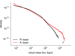
Figure 3: The probability density distribution of the lifetime average cloud base mass fluxes. Cloud are sampled from the 6th to 22nd hour from the simulation start in the R-base case, and from the 9th to 12th hour after the simulation start in the A-base case. Clouds with mass flux values lower than 600 kg/s are discarded from the plot to remove possible numerical noise, since those are mostly the clouds that cover only a single grid cell. 95 % confidence bands are plotted as shaded areas.

To represent conditions over land, a second reference case (A-base) is set up based on the Atmospheric Radiation Measurement (ARM) campaign, as in Brown et al. (2002). This case is forced by the averaged observed conditions at the Southern Great Plains (SGP) site on 21. June 1997. The start of the simulation is set to 11:30 UTC (6:30 am by local time), a time before convection initiates, and is integrated over a single diurnal cycle until 02:00 UTC next day (21:00 pm by local time). The initial vertical profiles of the thermodynamics quantities are computed based on the averaged soundings from that day (Fig. 1 in Brown et al. 2002). The wind direction did not change significantly during that day, so the initial wind profile is set to a constant wind of $u=10$ m s^-1 and $v=0$ m s^-1 at all levels. The geostrophic wind is also set to these values, while the background wind is set to $u=0$ m s^-1 and $v=7$ m s^-1. At the surface, the turbulent heat fluxes are prescribed following Brown et al. (2002) (see their Fig. 3) and exhibit a strong diurnal cycle. Weak large-scale forcing tendencies due to horizontal advection of moisture and temperature as well as radiative cooling rates are prescribed following the diurnal cycle; however they have only a minor impact on the simulation.

The two reference LES cases, R-base and A-base, are further modified to test the effects of surface conditions, diurnal cycle and large-scale forcing on the cloud statistics (Table 1). For all LES cases the simulations are performed over a domain of 51.2 km $\times$ 51.2 km, with a horizontal grid spacing of 25 m and a vertical resolution of 25 m up to a height of 5 km (domain top). Five vertical grid levels are used as damping layers at the top of the domain.

In the first group of simulations (R-base, R-0.24, R-0.33, A-base, A-0.5, A-0.1, A-0.06, and A-0.03; Figure 1), we have prescribed a range of values of the ratio of the sensible to latent heat fluxes at the surface, the Bowen ratio, to both cases starting from $B=$ 0.03 to $B=$ 0.5. This range of values is selected because it encompasses the typical values of $B$ characteristic for the regions of the tropical oceans to midlatitude continental conditions. The purpose of these simulations is to investigate the hypothesis that the differences between the two reference cases come from different Bowen ratios. The average Bowen ratio in R-base is around 0.03 and is approximately constant, while in A-base the starting value of B is around 0.3, and it decreases slightly over the diurnal cycle (Figure 1a). The two simulations based on RICO, R-0.24 and R-0.33, are set up by fixing the surface heat fluxes instead of the fixed SST. The total heat flux magnitude is kept equal to the reference RICO case, but the ratio of sensible to latent heat flux is changed to result in the wanted B value, 0.24 in the first and 0.33 in the second case. In the ARM-based cases (A-0.5, A-0.1, A-0.06, and A-0.03) the total surface heat fluxes are kept the same, but the ratio of sensible to latent heat flux is changed to result in the targeted B values of 0.5, 0.1, 0.06, and 0.03. These new B values are set at the beginning of the diurnal cycle, and are decreasing over the cycle at the same rate as in A-base (see Figure 1a). Note that the total surface heat flux in the RICO-based cases is in average more than twice lower than the total surface heat flux in the ARM-based cases (Table 1). By comparing the maximum values of the total surface heat flux or of the buoyancy flux near the peak of the diurnal cycle (Figs. 1b-d), the difference between the two reference cases is even up to four times.

As expected, the mean thermodynamic state of the subcloud layer is affected by the changes in the Bowen ratio. Increase of the Bowen ratio from 0.03 to 0.33 in the RICO-based cases causes an increase of the liquid water potential temperature by 1 K, and a decrease in the total water mixing ratio by 1 g/kg, as averaged over a 500 m thick layer starting from the surface. In the ARM case, a decrease of the Bowen ratio from 0.33 in A-base to 0.03 in A-0.03 causes a decrease of the liquid water potential temperature by 2 K, and an increase of the total water mixing ratio by 2 g/kg, averaged over a 500 m thick layer at the surface. Clearly, all these test cases have a different thermodynamic state in the boundary layer, even though the Bowen ratios might have the same values.

The depth of the subcloud layer is controlled by the surface buoyancy flux $F_{buoy}$ (Stevens 2007) with the higher cloud base heights in the simulations with higher surface buoyancy fluxes (Figs. 1d and 1e). The rate of growth of the subcloud layer is also influenced by $B$ and it is higher in the cases with higher $B$ (Figure 1e, see also Schrieber et al. 1996). Convective clouds are initiated sooner for the higher values of $B$ (Figure 1f). Except for the R-base case where the surface fluxes are not fixed, the top of the cloud layer does not seem to be significantly influenced by the changes in $B$ or $F_{buoy}$ (Figure 1f). This indicates that the processes in the cloud layer are to some extent detached from the surface forcing.

In the second group of simulations (A-lowflx, A-short, A-long; Figure 2), we have kept the Bowen ratio to its assigned values, but changed other key aspects of the forcing that are distinct between the two reference cases. The effect of the diurnal cycle in ARM is tested by shortening it by 1/3 (A-short), or by prolonging it by 1/3 (A-long), by applying these changes to the cycle period of the surface fluxes (see Figs. 2b,c) and the large-scale forcing tendencies. The effect of the value of the total surface heat flux is tested by reducing it by 20% in ARM (A-lowflx). As can be seen in Figure 2e, the rate of the growth of the cloud base height is not affected by these changes. However, if there is more time for the cloudy boundary layer to develop, as in A-long, a higher cloud base height is reached. The cloud layer deepens further either with an increase in the forcing period or with stronger total surface heat fluxes, although the differences are only around 100 m (Fig. 2f).

Cloud tracking

The cloud tracking algorithm developed by Heus and Seifert (2013) is applied to the simulated cloud fields in post-processing of the LES simulations. In the tracking algorithm, clouds are identified as the adjacent grid points that hold the liquid water path exceeding a threshold value of 5 gm^-2. In that way, the identified cloud area is a projection of a cloud from all vertical levels that can be tracked through space and time. Using the temporal resolution of one minute, cloud areas, vertical velocities and cloud lifetimes are recorded for each cloud in the simulation. A cloud splitting algorithm is then used to separate and track the individual cloud elements that form the multicore clouds or the merged cloud clusters. These cloud elements are defined as holding a buoyant core with the maximum incloud virtual potential temperature $\theta_{v}$ excess larger than a chosen threshold of 0.5 K. More details and validation of the tracking method are provided in Heus and Seifert (2013).

To develop a cloud parameterization based on the mass flux approach, the cloud mass flux has to be estimated near the cloud-base level. For this reason, we have developed a secondary tracking routine, as in Sakradzija et al. (2015), in which we record the area that every cloud occupies at the level that lies 100 m above the lifting condensation level (LCL). We define this area as the area that contains all the points with liquid water content greater than zero.

3 Cumulus cloud population statistics

The upward flux of mass through cloud base of the i-th cloud is defined as

$$m_{i}=\rho a_{i}w_{i}$$ (1)

where $a_{i}$ is the area [m²] occupied by points holding liquid water at a level 100 m above LCL and $w_{i}$ [m s^-1] is the vertical velocity averaged over the area $a_{i}$. To compute the distribution of the cloud mass flux, $p(m)$, we average $m_{i}$ over the lifetime of each cloud. Similar results can nevertheless be obtained by looking at the instantaneous values. The choice of computing the lifetime averaged mass fluxes comes from the possibility to reconstruct cloud lifecycles for the purpose of a parameterization, as in Sakradzija et al. (2015).

The distribution of cloud base mass fluxes is calculated for the two reference cases, RICO and ARM (Fig. 3). The probability density distribution is computed using the generic R function hist (R Core Team 2015). The width of the bins used to compute the probability density of mass fluxes is logarithmically increasing with higher mass flux values. The sampling period in RICO is from the 6th to the 22th hour of simulation, while in the ARM case clouds are sampled from the 6th (17:30 UTC) to the 12th (23:30 UTC) simulation hour. Only those clouds that were initialized during the sampling period are included in the calculation. Clouds that lasted longer than this sampling time period are followed beyond the time limit to finalize their lifecycles. The sample size of the lifetime average cloud base mass flux distribution is 317 014 clouds in the RICO case, and 120 292 clouds in the ARM case.

The two reference LES cases exhibit distinct horizontal and vertical extents of the clouds, number of clouds and their spacing, due to different initial conditions, surface and large-scale forcing. The mass flux distributions corresponding to these two reference cases have different shapes and they cover different ranges of the mass flux values (Fig. 3). The distribution of the cloud base mass flux in the ARM case shows a straight line shape on a log-log plot, similar to a power-law distribution over a range of three orders of magnitude. In contrast, the distribution in the RICO case shows a more concave shape. In previous literature on the cloud size distribution, such type of a concave shape has often been identified as a double power-law distribution with two distinct slopes and a scale-break point at the intermediate cloud size (Cahalan and Joseph 1989; Sengupta et al. 1990; Nair et al. 1998; Benner and Curry 1998; Neggers et al. 2003; Trivej and Stevens 2010; Heus and Seifert 2013). To make a parallel to these studies, we identify the scale-break in the mass flux distribution of the R-base case at a value of the cloud base mass flux close to $1\cdot 10$⁵ kgs^-1 (Fig. 3). Based on the qualitative comparison of the mass-flux distributions of the R-base and A-base case, we conclude that there is no universality in the distribution slopes on a log-log plot (Fig. 3). As we will show in section 4c, the slope of the mass flux distribution changes with the change of a control parameter of the simulations.

The sampling variability of the mass-flux distributions is very low in both reference cases except near the end of the right tails of the distributions (Fig. 3), which is a sign of a limited sample size of the largest possible cloud mass flux values. This portion of the distribution tail has higher sampling variability based on the 95 % confidence intervals computed for each distribution bin (shaded areas in Fig. 3). The confidence intervals were calculated using a bootstrap method with replacement using 1000 random samples.

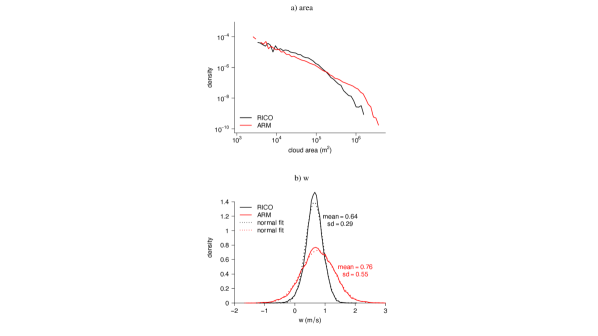
Figure 4: The probability density distribution of a) lifetime averaged cloud base areas and b) vertical velocity through cloud base. As in the previous figure, clouds with mass flux values lower than 600 kg/s are discarded from the plot to remove possible numerical noise.

As a key contributor to the cloud base mass flux, the cloud area $a_{c}$ is distributed qualitatively similarly to the distribution of the mass flux (Fig. 4a). The difference between the two reference LES cases shows similar characteristics as for the two mass flux distributions. So, the knowledge about the physical mechanism that shapes $p(m)$ might also be sufficient to describe $p(a_{c})$. The cloud area distribution of the A-base case shows a power-law-like shape with a scale-break around the value of 10⁶ m². The scale break in the ARM-base case is located at a scale an order of magnitude larger than the one of the R-base case. These two cloud area distributions are actually very similar to the two typical cloud size distributions observed over land and over ocean as derived from the Landsat images in Sengupta et al. (1990), their Fig. 4. A similar change in the distribution behaviour for the largest cloud areas is observed in the radar echo areas distribution in Trivej and Stevens (2010). Different statistics of the large echoes compared to a power-law behaviour of the small echoes may be controlled by the meteorological environment. In particular, the existence of an inversion layer topping the cloud layer limits the growth of clouds beyond a certain size, which can be connected to the observed break in the scaling (Trivej and Stevens 2010). Strong subsidence inversions over the tropical oceans might explain the position of the scale-break at the lower values than what is observed at midlatitudes (see also Wood and Field 2011).

The distribution of vertical velocity of individual clouds is approximately symmetric and can be well fitted using a normal distribution, as illustrated in Fig. 4b. The average vertical velocity per cloud is $\langle w\rangle=0.64$ in the RICO case and $\langle w\rangle=0.76$ in the ARM case. Compared to the RICO case, in the ARM case the variance of $w$ is significantly higher and some clouds can gain velocities larger than 2 m/s. This result is in line with the findings of Xu and Randall (2001), albeit for deep convection, where the most significant differences in the updraft intensities between tropical oceanic and midlatitude continental convection were found in the strongest 10% of the updrafts, not in the median values. The correlation between vertical velocity $w_{i}$ of individual clouds and their mass fluxes $m_{i}$ is very low (not shown here). This is the reason for the similarity between $p(m)$ and $p(a_{c})$, while $p(w)$ belongs to a different family of distributions.

Why are the two reference population distributions different? Is the distribution shape changing under the influence of the large-scale forcing or of the surface conditions? We address these questions in the following section.

4 The three hypotheses

The main differences between the two reference LES cases are in the existence of a strong diurnal cycle over land, strong self-organization of clouds over ocean and in the magnitude and partitioning of the surface turbulent heat fluxes (Table 1). Other aspects of the large-scale forcing are as well different between the two reference cases. However, we rule out those differences as a cause of the different distribution shapes because it was hypothesised and shown in previous studies that the intensity of the convective updrafts was insensitive to changes in the large-scale forcing (e.g. Robe and Emanuel 1996; Cohen and Craig 2006; Plant and Craig 2008). Based on these facts, we propose the three hypotheses that might explain the divergence of the mass flux distribution between the two reference LES cases:

1. diurnal cycle of convection determines the distribution $p(m)$,

2. convective self-organization determines the distribution $p(m)$, and

3. surface fluxes determine the distribution $p(m)$.

In the following, we test the three hypotheses by analysing all eleven LES cases (Table 1).

4.1 The first hypothesis: diurnal cycle of convection

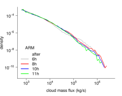
Figure 5: The probability density distribution of the lifetime average cloud base mass flux sampled over time frames of one hour duration over the diurnal cycle of the A-base case, starting after 6, 8, 10 and 11 hours of simulation (at 17:30 UTC, 19:30 UTC, 21:30 UTC, and 22:30 UTC).

Here we test if changes in the forcing associated with the convective diurnal cycle might be responsible for the different shapes of $p(m)$ in the two reference cases. We sample the clouds that emerge in the ARM case during four time frames of one hour duration, taken at different stages of the diurnal cycle, starting at 17:30 UTC. The distribution of cloud base mass flux in all four time frames is shown in Fig. 5. It is clear that there is no significant change in $p(m)$ over the diurnal cycle of the ARM case, i.e. the distribution $p(m)$ is stationary.

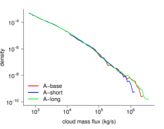
Figure 6: The probability density distribution of the lifetime average cloud base mass flux over the cases with different diurnal cycle periods, based on the ARM case.

Another property of the diurnal cycle that might influence $p(m)$ is the period of the diurnal cycle. Shorter or longer diurnal cycles imply faster or slower temporal changes in the forcing. With faster changes, clouds might have less time to develop undisturbed, so their sizes and mass fluxes might be lower. Or, with slower changes in the forcing, larger clouds might result. To test this, we investigate the results of the simulations A-short and A-long. A time frame of one hour duration is taken around the peak of the diurnal cycle, after 9, 7 and 11 hours from simulation start in A-base, A-short, and A-long, respectively, and $p(m)$ is examined (Fig. 6). There is again no significant difference among the simulations, except near the right tail of the distribution, where the A-short case shows a faster drop-off than the other two cases. This means that the largest possible clouds cannot develop in the ARM case if the period of the forcing is too short. Overall, there is nevertheless no change in the distribution shape, and the slope of the line stays similar across the three cases. The results of these experiments demonstrate that changes of the forcing over a diurnal cycle do not shape the distribution of the cloud base mass flux.

4.2 The second hypothesis: convective self-organization

In this section we test how the spatial correlations during the organized phase of the RICO case influence the cloud base mass flux distribution. Organization of convective clouds into clusters, lines, or arcs could influence $p(m)$ by affecting the size and intensity of individual cloud elements. Here, it is important to note that the cloud tracking routine identifies the cloud entities that form the cloud clusters, and performs splitting so that every element can be followed separately even when two cloud elements have merged. In contrast, past studies have investigated the distributions of merged cloud clusters and suggested self-organization as a mechanism for creating power-laws (Scheufele 2014).

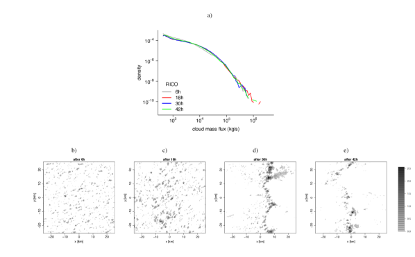
Figure 7: The probability density distribution of the lifetime average cloud base mass flux in the R-base case, over different stages of cloud organization. The corresponding horizontal spatial distribution of the cloud field is visualized in (b-e) using the liquid water path [g m^-2].

We choose the R-base case to test the effects of cloud organization on $p(m)$ because this convective case is strongly organized after one day of simulation (Fig. 7). Starting from a randomly distributed field of clouds and looking into the time frames with different stages and forms of organization, we plot $p(m)$ in Fig. 7. We find no evidence that self-organization of clouds has an effect on $p(m)$ because the overall distribution shape stays the same in spite of organization. Hence, the different degrees of organization between RICO and ARM cannot explain the differences in $p(m)$.

Even though self-organization is not responsible for the final shape of the distribution, it is a process that can produce longer tails in the cloud distributions, if the cloud splitting is not performed and cloud clusters are sampled to compute $p(m)$ (Scheufele 2014). Fig. 7 indicates that this dependency vanishes if individual cloud elements are considered.

4.3 The third hypothesis: surface heat fluxes

The two reference cases have very different surface conditions, one is set over the ocean, while the other one is set over land, so the magnitudes of the surface heat fluxes differ by up to a factor four between the cases (see Fig. 1). We investigate here the dependency of the distribution shape on the surface turbulent heat fluxes, which drive the boundary layer convective updrafts that ultimately form cumulus clouds at the top of the subcloud layer. We test the magnitude of the fluxes and their partitioning at the surface.

4.3.1 The magnitude of the surface heat fluxes

We have already concluded in the previous section for the ARM case that $p(m)$ does not change over a single diurnal cycle (Fig. 5). From this conclusion it also follows that $p(m)$ is not sensitive to the surface flux magnitude. To further prove this, we perform one additional test (A-lowflx) in which the total surface turbulent heat flux is lowered by 20 % (Fig. 8). There is no significant difference between the two distributions. The A-lowflx case can simply be considered as another realization of the same shallow cloud ensemble of the A-base case.

4.3.2 The ratio of the surface heat fluxes, $B$

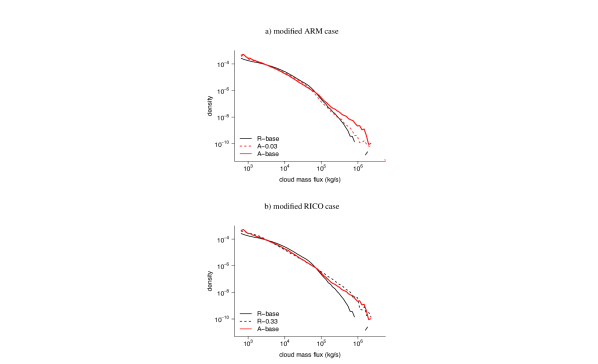
Figure 9: Reproduction of the distribution shape of the lifetime average cloud base mass flux of a) the R-base case by altering the Bowen ratio of the ARM case to $B=0.03$, and b) of the A-base case by altering the RICO case Bowen ratio to $B=0.33$.

The ratio of the sensible and latent heat fluxes at the surface, the Bowen ratio $B$, is the main parameter that characterizes the two surface types, ocean and land. Though the total surface flux magnitude has no effect on $p(m)$, the partitioning of this flux into sensible and latent heating might have an effect. Note that the Bowen ratio does not change much over the diurnal cycle in ARM. We thus turn our attention to the sensitivity experiments using different Bowen ratios (Fig. 9).

By changing only the ratio of the surface fluxes and leaving their magnitudes unchanged, the shape of the mass flux distribution can be altered. More importantly, by setting the RICO Bowen ratio in the ARM set-up (A-0.03), the mass flux distribution of the RICO case is recovered (Fig. 9a). Likewise, by setting the ARM Bowen ratio in the RICO set-up (R-0.33), the mass flux distribution of the ARM case is recovered (Fig. 9b). Thus, it is evident that the ratio of the surface fluxes and not their magnitudes shapes the mass flux distribution.

4.3.3 The two modes of the cloud distribution

The final shape of $p(m)$ is a result of the superposition of the distribution modes associated with cloud groups of different subtypes: active, forced and passive clouds (see the classification of Stull 1985). We examine the dependency of these modes on the Bowen ratio separately. Here we simplify the classification of clouds into buoyant (active) and non-buoyant (passive) clouds, as in Sakradzija et al. (2015). Forced clouds fall into the ”passive” non-buoyant cloud group owing to this simplification. Clouds are classified as active buoyant clouds if the excess of the vertically integrated virtual potential temperature within clouds, $\theta_{v,up}-\overline{\theta_{v}}$, is larger than a threshold. The threshold is set to 0.5 K, except in a case where this leads to a too small statistical sample, as in R-0.33. In the latter case, the threshold is set to 0.4 K.

In the RICO-base case (Fig. 10a), the cloud distribution shows shorter tails in both modes, and lower mass fluxes in average compared to the A-base case (full lines in Fig. 10b). With increasing Bowen ratio, the active cloud modes shift towards higher mass flux values, while the slopes of the two modes become less steep (Fig. 10). Through the control on the range of mass flux values that individual modes of $p(m)$ can take, and by setting the slope of the modes, the Bowen ratio ends up determining the average mass flux per cloud $\langle m\rangle$ in both distribution modes.

This fact might explain why different power-law slopes are documented in different observational studies of cloud population (see Table 1 in Zhao and Di Girolamo 2007). The slopes of the observed cloud size distributions in the midlatitude regions have lower values than the slopes in the tropics (see Wood and Field 2011). These characteristics of the observed cloud size distribution correspond to the control that $B$ imposes on the slopes that we observe in the RICO and the ARM cloud-base mass flux distributions (Fig. 10). Higher values of $B$ in midlatitudes produce lower slopes compared to the higher slopes that are produced as a result of low $B$ in the tropics.

5 The Bowen ratio indirectly sets the average mass flux per cloud

To understand the link between $p(m)$ and $B$, we aim at deriving in this section the constraints on the mass flux $\langle m\rangle$ that an average cloud can transport based on the boundary layer energetics. As will be shown in section 6, $\langle m\rangle$ is the key parameter through which the difference between the mass flux distributions of the two reference cases is set.

We start from the concept of atmospheric convection as a natural heat engine (Rennó and Ingersoll 1996). During a heat cycle of an average convective cloud, the heat $Q_{in}$ [J] is input near the surface in the form of the turbulent surface heat flux $F_{in}$ [Wm^-2] (sum of latent and sensible heat fluxes). This heat is partly converted into mechanical work $W_{mech}$ of the convective overturning in the subcloud layer, and the rest is added into the cloud layer and redistributed further. Here, we define the heat cycle for the subcloud layer that lies between the surface layer over the warm ocean or land surface and the colder cloud layer above.

The efficiency of the heat cycle is defined as the ratio of mechanical work and the heat input at the surface

$$\eta=\frac{W_{mech}}{Q_{in}}$$ (2)

The theoretical maximum efficiency of the heat cycle in the subcloud layer is the Carnot efficiency, which can be defined as

$$\eta_{max}=\frac{T_{sfc}-T_{lcl}}{T_{sfc}}$$ (3)

$T_{sfc}$ is the surface temperature and $T_{lcl}$ is the temperature at the lifting condensation level. If the heat input at the surface would happen solely in form of the sensible heat flux and if no heat was spent to transport water vapor out of the subcloud layer, the efficiency of the convective heat cycle would approach the Carnot efficiency. However, the thermodynamic cycle of convection in the boundary layer is a mixed moist heat cycle with an efficiency that is lower than the maximum theoretical Carnot efficiency, $\eta<\eta_{max}$. As shown in Shutts and Gray (1999), the efficiency of the moist heat cycle can be expressed as (see their Eq. 19)

$$\eta=\frac{B}{1+B}\left(1+\frac{\epsilon c_{p}T_{sfc}}{L_{v}B}\right)\frac{gH}{2c_{p}T_{sfc}}.$$ (4)

where $c_{p}$ is the specific heat capacity of the dry air at constant pressure, $L_{v}$ is the latent heat of vaporization, $g$ is the gravitational acceleration, $\epsilon=1-R_{v}/R_{d}=0.608$, $R_{v}$ is the gas constant for water vapour, $R_{d}$ is the gas constant for dry air, and $H$ is the subcloud layer depth. Eq. 4 is derived under the assumption that the effective heat input at the surface, $\eta F_{in}$, is used to maintain convection against mechanical dissipation in a convective system in statistical equilibrium. The efficiency of a moist heat cycle $\eta$ could be further explained using the entropy budget analysis as in Pauluis and Held (2002). They found that convection acts both as a heat cycle and as an atmospheric dehumidifier, and the irreversible entropy production by the two processes are in competition. The more the atmosphere acts as a dehumidifier, the less effective it is to generate kinetic energy of convective circulations (Pauluis and Held 2002).

From Eq. 4, it follows that the Bowen ratio highly influences the fraction of the heat input that can be transformed into mechanical work to maintain convective circulations. $B$ appears explicitly in Eq. 4 but also implicitly through its control on the depth of the subcloud layer $H$ (see Schrieber et al. 1996; Stevens 2007).

Equation 2 does not explicitly relate $\langle m\rangle$ to the moist heat cycle. To do so, we proceed as follows. The average cloud-base mass flux per cloud $\langle m\rangle$ is related to the turbulent flux of the moist static energy at the cloud-base level $\rho\overline{w^{\prime}h^{\prime}}$ through the mass flux approximation as defined in Arakawa and Schubert (1974):

$$\rho\overline{w^{\prime}h^{\prime}}\approx\sum_{i}m_{i}(h_{i}-\overline{h})$$ (5)

where $i=1,...,N$ is the index of individual clouds, and $h_{i}-\overline{h}$ is the excess of the moist static energy within the updrafts that form clouds with respect to the environment, and an overline denotes averaging over the domain.

As a first simple hypothesis, we assume that the turbulent flux of the moist static energy at cloud base, $\rho\overline{w^{\prime}h^{\prime}}$, is proportional to the effective surface forcing of the cloud ensemble, $N\eta F_{in}$, and by using Eq. 5 we write

$$\sum_{i}m_{i}(h_{i}-\overline{h})\approx C_{1}~{}N\eta F_{in}$$ (6)

where $C_{1}$ is a proportionality constant, which can be seen as a factor of correction for further heat losses not taken into account, and $N$ is the number of clouds in the cloud ensemble. Because the surface forcing is homogeneous, $F_{in}$ is equal for all individual cloud heat cycles. The efficiency is controlled by the homogeneous surface properties and the subcloud layer depth and is approximately equal among the clouds (see Eq. 4), so $\eta$ is treated as a constant in a single convective case. Now we apply the mass-flux-weighted averaging as defined in Yanai et al. (1973) to Eq. 6

$$\frac{\sum_{i}m_{i}h_{i}}{\sum_{i}m_{i}}\approx\tilde{h}$$ (7)

$\tilde{h}$ is the mass-flux-weighted average of $h$, which is approximately equal to the average of the moist static energy per cloud, $\langle h\rangle$, where the brackets $\langle.\rangle$ denote averaging over the cloud ensemble. The relative difference between the values of $\tilde{h}$ and $\langle h\rangle$ is lower than 0.5 % as estimated from LES. So, we can rewrite the left-hand side of Eq. 6 as

$$\sum_{i}m_{i}(h_{i}-\overline{h})=\sum_{i}m_{i}h_{i}-\sum_{i}m_{i}\overline{h}=\frac{\sum_{i}m_{i}\sum_{i}m_{i}h_{i}}{\sum_{i}m_{i}}-\sum_{i}m_{i}\overline{h}\approx\sum_{i}m_{i}(\langle h\rangle-\overline{h})$$ (8)

$$\sum_{i}m_{i}(\langle h\rangle-\overline{h})\approx C_{1}~{}N\eta F_{in}$$ (9)

An average moist heat cycle per cloud can then be expressed as

$$\langle m\rangle(\langle h\rangle-\overline{h})\approx C_{1}~{}\eta F_{in}$$ (10)

and the average mass flux per cloud is then approximately equal to

$$\langle m\rangle\approx C_{1}~{}\frac{\eta F_{in}}{\langle h\rangle-\overline{h}}.$$ (11)

with $\eta$ given by Eq. 4.

We look into the LES simulations to find evidence to support Eq. 11. We base our analysis on the active cloud group and we plot the average mass flux per active cloud $\langle m\rangle$ versus the right-hand side of the equation 11 (Fig. 11a). It turns out that Eq. 11 holds remarkably well for the eight tested LES cases of Table 1, which suggests that the average mass flux per cloud is determined by the moist heat cycle of the subcloud layer. The coefficient of determination of a linear regression model is $r^{2}=0.95$. The slope is estimated to be equal to $C_{1}=0.13$. The intercept parameter is nevertheless not equal to zero and results in an additional mass flux which we will denote by $m_{0}$:

$$\langle m\rangle=m_{0}+C_{1}~{}\frac{\eta F_{in}}{\langle h\rangle-\overline{h}}$$ (12)

The estimated value in this study is $m_{0}=3\cdot 10^{-5}$ kg/s/m². Depending on the test case and the Bowen ratio value, $\langle m\rangle$ can be 1.5 to 6.9 times larger than $m_{0}$ (Fig. 11a).

The scaling Eq. 11 is evaluated in Fig. 11a only for the active clouds, while we do not show the scaling for the ”passive” cloud group. This is because the buoyancy threshold used to separate the clouds into the two groups misinterpret some active clouds as passive. We can however show the scaling for the total cloud ensemble in Fig. 11b, which still holds.

Equation 11 is decomposed into two parts to test the dependency of $\langle m\rangle$ of the active clouds on $\frac{~{}F_{in}}{\langle h\rangle-\overline{h}}$ and $\eta$ separately (Fig. 11c,d). It is clear from Fig. 11c that $\langle m\rangle$ does not scale with $\frac{~{}F_{in}}{\langle h\rangle-\overline{h}}$. The points are aligned vertically in three different groups associated with the three main values of the ratio $\frac{~{}F_{in}}{\langle h\rangle-\overline{h}}$, i.e. 0.05, 0.08, and 0.13. The increase in $\langle m\rangle$ in each of these three groups of points is due to changing values of $B$. Thus, $\langle m\rangle$ is controlled by $B$, while the different mean states of the subcloud layer can still result in the same value of $\langle m\rangle$. It is not shown here explicitly, but $\langle m\rangle$ also does not scale uniquely with the total surface heat flux $F_{in}$.

The average mass flux per cloud $\langle m\rangle$ is also not uniquely determined by $\eta$. $\eta$ sets the slope of the three lines corresponding to the three different magnitudes of the ratio $\frac{~{}F_{in}}{\langle h\rangle-\overline{h}}$. Furthermore, if the ratio $\frac{~{}F_{in}}{\langle h\rangle-\overline{h}}$ in a given group of points is higher, the efficiency $\eta$ in the same group is lower compared to the other groups. As a result, $\langle m\rangle$ is uniquely determined by the product of the two factors (Eq. 11), with $\eta$ playing the key role in setting the dependence on $B$.

The fact that $B$ sets the efficiency of the moist convective heat cycle, and thus also controls the expected value of $p(m)$, directly explains why the magnitude of the surface forcing does not influence the distribution shape. From this it also follows that changes of the surface forcing over the diurnal cycle can not alter the distribution shape, as long as $B$ does not change significantly over the diurnal cycle. The moist heat cycle formalism might also explain why self-organization is not a powerful driver for the distribution $p(m)$. The convecting system is forced by the same amount of heat input and the efficiency of the moist heat cycle is the same at all stages of cloud organization. So, for the shape of $p(m)$, the spatial distribution of clouds does not play any significant role.

An important point to notice here is that the heat cycle formalism applies to the average convective cycle per cloud, and thus it determines $\langle m\rangle$, not the bulk contribution $M$ of all clouds in the shallow cloud ensemble. $M$ is not fully constrained by the heat cycle of the subcloud layer. This has an implication for the bulk closure assumptions in parameterization of convection. To retrieve the closure of a bulk parameterization, an average mass flux per cloud $\langle m\rangle$ has to be multiplied by the total number of clouds $N$ to result in the bulk mass flux $M$. Therefore, the controls on $M$ may be decomposed into two contributions: the surface conditions control $\langle m\rangle$, while in addition to the surface conditions the large-scale forcing acts to set the number of clouds in the ensemble $N$.

6 Parameters of the mass flux distribution

For the application to parameterizations based on the spectral cloud ensembles (Arakawa and Schubert 1974) or stochastic cloud ensembles (as in Plant and Craig 2008; Sakradzija et al. 2015), a functional form for $p(m)$ has to be defined and the corresponding distribution parameters have to be estimated. In the following, we adopt the mixed Weibull distribution as a functional form for $p(m)$ as in Sakradzija et al. (2015)

$$\begin{split}p(m)=(1-f)\frac{k_{p}}{\lambda_{p}}\left(\frac{m}{\lambda_{p}}\right)^{k_{p}-1}e^{-\left(m/\lambda_{p}\right)^{k_{p}}}+\\ f\frac{k_{a}}{\lambda_{a}}\left(\frac{m}{\lambda_{a}}\right)^{k_{a}-1}e^{-\left(m/\lambda_{a}\right)^{k_{a}}}\end{split}$$ (13)

where $f$ is the fraction of active cumulus clouds, $k$ is the shape and $\lambda$ is the scale parameter of the Weibull distribution, and subscripts _p and _a denote passive and active distribution modes.

From the results of the previous section we know that $\langle m\rangle$ varies with the surface conditions. The question nevertheless remains whether any of the remaining distribution parameters, namely $k_{p,a}$ and $\lambda_{p,a}$, are universal constants. In the study of Sakradzija et al. (2015) these parameters were estimated only for the RICO case for the time period of six hours, starting after six hours of simulation. The estimated shape parameter was $k_{p}=k_{a}=0.7$ for the given cloud sample. In the following, we extend the analysis over longer time period of the RICO case, and over land conditions in the ARM case. In the following we focus on the estimation of the shape parameters, $k_{p,a}$, while the scale parameters of the Weibull distribution modes, $\lambda_{p,a}$, can be calculated from the expected value of the distribution, $\langle m\rangle_{p,a}=\lambda_{p,a}\Gamma[1+1/k_{p,a}]$.

In shallow cumulus cloud ensembles, the shape parameter that is less than one, $k<1$, indicates that the memory of cloud lifecycles has an effect on the distribution shape (Sakradzija et al. 2015). This effect takes place through correlation between the cloud lifetimes $\tau_{i}$ and the cloud base mass fluxes $m_{i}$, which is already demonstrated for the RICO case in Sakradzija et al. (2015). We confirm this finding for the RICO case, and we also show that it holds in the ARM case (Fig. 12). This correlation is high with the correlation coefficient equal to $r_{p}=0.8$ in RICO and $r_{p}=0.9$ in ARM, estimated for the active cumulus clouds. We assume that this correlation can be described by a power law relation $\tau/\langle\tau\rangle=(m/\langle m\rangle)^{\beta}$, where $\beta$ is the power exponent, and $\langle\tau\rangle$ is the average cloud lifetime, as in Sakradzija et al. (2015).

In the theory of extreme events, it is known that long-term correlations with a power-law decay of the autocorrelation function lead to Weibull distributions of return intervals between rare events (e.g. Bunde et al. 2003; Blender et al. 2015). In that case the power-law exponent of the autocorrelation function, $t^{-\beta}$, can be assumed equal to the shape parameter of the Weibull distribution, $k$ (e.g. Blender et al. 2015). Following this reasoning, the normalized lifetime expression $\tau/\langle\tau\rangle=(m/\langle m\rangle)^{\beta}$ also leads to a Weibull distribution for the cloud base mass flux distribution (Eq. 13). The power-law exponent can then be related to the shape parameter of the active mode of the Weibull distribution as $k_{a}\approx\beta$. The nonlinear least square fit in Fig. 12 gives the values for the exponent $\beta=0.8$ in RICO and $\beta=0.77$ in ARM. Hence, it appears that $\beta$ is independent on the case set-up. The passive cloud group is more dispersive (not shown here) and the statistical fit is thus more uncertain, however we will assume that $k_{p}\approx k_{a}=0.8$.

Combination of the two Weibull modes of the same shape parameter $k_{p}=k_{a}=k$, but different $\langle m_{p}\rangle$ and $\langle m_{a}\rangle$, and hence different $\lambda_{a,p}$, can explain the difference between the two cases (Fig. 13). To construct Fig. 13 and in the purpose of highlighting the uncertainties in $p(m)$ due to the chosen value of $k$ only, we here calculate the values of $\langle m_{p}\rangle$ and $\langle m_{a}\rangle$ directly from the LES output rather than using the formalism of a thermodynamic cycle. The chosen value of $k_{p}=k_{a}=0.8$ provides a good fit to both distributions (Fig. 13). On the same plot, we also test a broad range of values for $k$, which demonstrates that $k$ is of secondary importance in determining the final shape of $p(m)$. It is evident that $k$ can still take a wide range of values, [0.8,1] for RICO and [0.5,0.8] for ARM, for the correct reproduction of the distribution $p(m)$. Therefore, we conclude that the main parameter that sets the difference in $p(m)$ among the shallow cumulus cases is $\langle m\rangle$.

The parameter $f$, which is the proportion that active clouds take in the cloud ensemble, is about 4 to 5 % of the total cloud population both in ARM and RICO. This is valid for the distribution of lifetime average mass fluxes during time frames of one hour duration, and including only those clouds that are initiated during the time frames. We choose here to set the value of $f$ to 0.05.

7 Conclusions

The probability distribution of cloud base mass flux $p(m)$ differs among shallow cumulus cases. These differences manifest themselves through various shapes, slopes and scales of the distribution. Based on the examination of one typical LES case over the ocean (RICO) and one typical LES case over land (ARM), and nine variations of these two cases, we propose an explanation for the differences in $p(m)$ among shallow cumulus cases.

The set-up of the two reference LES cases differs in the strength and partitioning of the surface turbulent heat fluxes, as well as in the prescribed large-scale forcing tendencies. The ARM case has a strong diurnal cycle that is typical for land conditions, while there is no diurnal cycle in the simulation over the ocean (RICO). In addition, the cloud field in the RICO case is strongly organized, with manifestation of cold pools and arc structures. We have investigated which of these differences in the LES set-up is responsible for the distinct shapes of the distribution $p(m)$.

Analysis demonstrates that partitioning of the surface turbulent fluxes into sensible and latent heating, the Bowen ratio $B$, is the only parameter that controls the shape of the distribution $p(m)$. This control appears to be governed by the second law of thermodynamics and can be explained by interpreting moist convection in the boundary layer as a combination of moisture and heat cycles (as in Shutts and Gray 1999; Pauluis and Held 2002). The efficiency of the moist heat cycle, $\eta$, is less than the Carnot cycle efficiency, because it is directly set by the surface Bowen ratio and the depth of the convecting layer (Shutts and Gray 1999). Through $\eta$, the Bowen ratio controls the average mass flux per cloud $\langle m\rangle$.

Using the formalism of a moist heat cycle, a scaling law for $\langle m\rangle$ is derived (see Eq. 11). By this scaling, the average vertical mass flux through cloud base $\langle m\rangle$ is proportional to the ratio of the effective surface heat flux $\eta F_{sfc}$ and the excess in the moist static energy at the cloud base with respect to the environment $\langle h\rangle-\bar{h}$. This scaling holds remarkably well for the active buoyant clouds in the eight considered convective cases, and thus suggests an universal law across a wide range of the control parameter $B$. Passive and forced clouds are not investigated here due to their uncertain separation from the active clouds, but we show that the scaling still holds considering all cloud types.

As such, $B$ controls the shape of the distribution $p(m)$ through its control on $\langle m\rangle$. We have demonstrated that different shapes of the distribution $p(m)$ can be well captured by a two-mode Weibull distribution function. The shape parameter of each distribution mode is $k<1$ and it is of secondary importance for determining the final shape of $p(m)$. The reason for this robustness comes from similarity of the power-law exponent $\beta$ in the relation between cloud lifetime and cloud-base mass flux across the LES cases. This power-law exponent sets the unique value of the shape parameter across the LES cases.

The Bowen ratios tested in this study covered the range of values between 0.03 and 0.5. This range corresponds to the span of conditions covering ocean surfaces to temperate forests and grasslands. In order to make the conclusions of this study more general, it would be advantageous to expand the study to dry land surfaces and to extend the analysis to cloud observations. In addition, the mechanical forcing in the two reference cases was of similar magnitude. A question left for further investigation is how stronger winds and higher wind shears might influence the convective mass flux and population statistics.

One of the key outcomes of this study is that the concept of a moist heat cycle applies to an average convective cloud cycle. In order to retrieve the total mass flux in a cloud ensemble $M$, it is necessary to set the constraints on the number of clouds $N$ in every given case, since $M=N\langle m\rangle$. $N$ does not appear to be constrained by the moist heat cycle. One may hypothesize that $M$ is governed by the large-scale forcing through control on the number of clouds $N$, in addition to the surface conditions that impose a constraint on $\langle m\rangle$.

The results of this study also have implications for the cloud size distribution, which has a very similar shape to the distribution $p(m)$. Various shapes and slopes of the cloud size distribution that are observed and have been documented in literature, may just reflect changes in Bowen ratios encountered across various studies. The various proposed distribution shapes could be encompassed by a single functional form given by the mixed Weibull distribution function. Such a multimodal distribution function already encompasses all the observed shapes, starting from an exponential shape to power-laws, depending on the value of the distribution parameters. Based on this study, the expected value of the cloud size distribution might impose the only relevant control on the distribution shape, which then could be constrained by the underlying physical processes in the boundary layer.

Table 1: List of the LES cases with the abbreviations used in the text, the case on which the simulations are based on, the maximum Bowen ratio $B_{max}$, the total surface turbulent heat flux averaged over the simulation period $\overline{F}_{in}=\overline{F_{sh}+F_{lh}}$, and the type and duration of the large-scale forcing $LS_{forc}$.

abbr.	reference case	$B_{max}$	$\overline{F}_{in}[W/m^{2}]$	$LS_{forc}$
R-base	RICO	0.06	171	$const.$
R-0.24	RICO	0.24	152	$const.$
R-0.33	RICO	0.33	152	$const.$
A-base	ARM	0.36	343	14 h 30’
A-0.5	ARM	0.50	340	14 h 30’
A-0.1	ARM	0.11	347	14 h 30’
A-0.06	ARM	0.06	348	14 h 30’
A-0.03	ARM	0.03	349	14 h 30’
A-lowflx	ARM	0.36	274	14 h 30’
A-short	ARM	0.36	341	10 h
A-long	ARM	0.36	344	19 h

Figure 1: Time series of the surface forcing in the first group of eight LES cases from Table 1: a) Bowen ratio $B$, b) surface sensible heat flux $F_{sh}$, c) surface latent heat flux $F_{lh}$, d) surface buoyancy flux $F_{buoy}$, and the resulting e) cloud base $z_{b}$ and f) cloud top heights $z_{t}$. The difference between these simulations is set through the Bowen ratio, which is indicated in the case abbreviations and line colours. Time from the start of the simulation is shown on the x axis.

Figure 2: Time series of the surface forcing in the second group of the LES cases based on ARM: a) Bowen ratio $B$, b) surface sensible heat flux $F_{sh}$, c) surface latent heat flux $F_{lh}$, d) surface buoyancy flux $F_{buoy}$, and the resulting e) cloud base $z_{b}$ and f) cloud top heights $z_{t}$. The difference between these simulations is set through the period of the large-scale forcing (A-short and A-long) and through the total surface heat flux magnitude (A-lowflx).

Figure 8: The probability density distribution of the lifetime average cloud base mass flux in the A-lowflx case compared to the distribution in the A-base case.

Figure 10: The lifetime average cloud base mass flux distribution of active and passive cloud modes for different Bowen ratios: a) RICO based cases, and b) ARM based cases. Full lines correspond to the reference cases, while dashed lines correspond to the cases with changed $B$.

Figure 11: Scaling of the average cloud base mass flux $\langle m\rangle$ based on the moist heat cycle (Eq. 11) for eight LES cases showing a) the average mass flux of active cumulus clouds, b) the average mass flux of the total cloud ensembles, and the right hand side of the Eq. 11 decomposed into c) ${F_{in}}/({\langle h\rangle-\overline{h}})$ and d) $\eta$. Two time frames are used for these figures, the frames starting after 6 and 10 hours of the simulation in the RICO based cases, and after 8 and 10 hours in the ARM based cases.

Figure 12: Scatter plot of individual active cloud lifetimes and cloud base mass fluxes normalized by the ensemble average values: a) R-base simulation and b) A-base simulation. Cloud samples are collected during one hour starting from the 10th simulation hour. The red line is a fit of the function $\tau/\langle\tau\rangle=(m/\langle m\rangle)^{\beta}$ using the non-linear least squares.

Figure 13: The mass flux distribution approximately fitted using a bimodal Weibull function. The distribution fit of RICO is shown in the upper plot a), while the distribution fit of ARM is shown in the lower plot b). The range of the shape parameter $k$ is quite wide to show low sensitivity of the distribution overall shape to this parameter, while the fraction of active clouds in the ensemble is $f=5$%.