Parallel-in-Space-and-Time Simulation of the Three-Dimensional, Unsteady Navier-Stokes Equations for Incompressible Flow

Abstract

In this paper we combine the Parareal parallel-in-time method together with spatial parallelization and investigate this space-time parallel scheme by means of solving the three-dimensional incompressible Navier-Stokes equations. Parallelization of time stepping provides a new direction of parallelization and allows to employ additional cores to further speed up simulations after spatial parallelization has saturated. We report on numerical experiments performed on a Cray XE6, simulating a driven cavity flow with and without obstacles. Distributed memory parallelization is used in both space and time, featuring up to 2,048 cores in total. It is confirmed that the space-time-parallel method can provide speedup beyond the saturation of the spatial parallelization.

1 Introduction

Simulating three-dimensional flows by numerically solving the time-dependent Navier-Stokes equations leads to huge computational costs. In order to obtain a reasonable time-to-solution, massively parallel computer systems have to be utilized. This requires sufficient parallelism to be identifiable in the employed solution algorithms. Decomposition of the spatial computational domain is by now a standard technique and has proven to be extremely powerful. Nevertheless, for a fixed problem size, this approach can only push the time-to-solution down to some fixed threshold, below which the computation time for each subdomain becomes comparable to the communication time. While pure spatial parallelization can provide satisfactory runtime reduction, time-critical applications may require larger speedup and hence need additional directions of parallelism in the used numerical schemes.

One approach that has received increasing attention over recent years is parallelizing the time-stepping procedure typically used to solve time-dependent problems. A popular algorithm for this is Parareal, introduced in LionsEtAl2001 and comprehensively analyzed in Gander2007 . Its performance has been investigated for a wide range of problems, see for example the references in Minion2010 ; RuprechtKrause2012 . A first application to the 2D-Navier-Stokes equations, focussing on stability and accuracy without reporting runtimes, can be found in FischerEtAl2005 . Some experiments with a combined Parareal/domain-decomposition parallelization for the two-dimensional Navier-Stokes equations have been conducted on up to 24 processors in Trindade2004 ; Trindade2006 . While they successfully established the general applicability of such a space-time parallel approach for the Navier-Stokes equations, the obtained speedups were ambiguous: Best speedups were achieved either with a pure time-parallel or a pure space-parallel approach, depending on the problem size.

In this paper we combine the Parareal-in-time and domain-decomposition-in-space techniques and investigate this space-time parallel scheme by means of solving a quasi-2D and a fully 3D driven cavity flow problem on a state-of-the-art HPC distributed memory architecture, using up to 2,048 cores. We demonstrate the capability of the approach to reduce time-to-solution below the saturation point of a pure spatial parallelization. Furthermore, we show that the addition of obstacles into the computational domain, leading to more turbulent flow, leads to slower convergence of Parareal. This is likely due to the reported stability issues for hyperbolic and convection-dominated problems, see FarhatEtAl2003 ; RuprechtKrause2012 .

2 Physical model and its discretization and parallelization

The behavior of three-dimensional, incompressible Newtonian fluids is described by the incompressible Navier-Stokes equations. In dimensionless form the according momentum- and continuum equation read
$\displaystyle\partial_{t}\mathbf{u}+\mathbf{u}\cdot\nabla\mathbf{u}$ $\displaystyle=\frac{1}{\textrm{Re}}\Delta\mathbf{u}-\nabla p$ $\displaystyle\nabla\cdot\mathbf{u}$ $\displaystyle=0$
with $\mathbf{u}=(u,v,w)$ being the velocity field consisting of the Cartesian velocity-components, $p$ being the pressure and Re the dimensionless Reynolds number.

The Navier-Stokes solver is based on the software-package NaSt3DGP NaSt3DGP ; GriebelDornseiferNeunhoeffer:1998 and we further extended it by an MPI-based implementation of Parareal LionsEtAl2001 . In NaSt3DGP, the unsteady 3D-Navier-Stokes equations are discretized via standard finite volume/finite differences using the Chorin-Temam Chorin ; Temam projection method on a uniform Cartesian staggered mesh for robust pressure and velocity coupling. A first order forward Euler scheme is used for time discretization and as a building block for Parareal, see the description in 2.1. Second order central differences are used for the pressure gradient and diffusion. The convective terms are discretized with a second order TVD SMART SMART upwind scheme, which is basically a bounded QUICK QUICK scheme. Furthermore, complex geometries are approximated using a first order cell decomposition/enumeration technique, on which we can impose slip as well as no-slip boundary conditions. Finally, the Poisson equation for the pressure arising in the projection step is solved using a BiCGStab BiCGStab iterative method.

2.1 Parallelization

Both the spatial as well as the temporal parallelization are implemented for distributed-memory machines using the MPI-library. The underlying algorithms are described in the following.

Parallelization in space via domain decomposition

We uniformly decompose the discrete computational domain $\Omega_{h}$ into $P$ subdomains by first computing all factorizations of $P$ into three components, i.e. $P=P^{x}\cdot P^{y}\cdot P^{z},$ with $P^{x},P^{y},P^{z}\in\mathbb{N}$. Then we use our pre-computed factorizations of $P$ as arguments for the following cost function $C$ with respect to communication

$$C(P^{x},P^{y},P^{z}) =\frac{I}{P^{x}}\cdot\frac{J}{P^{y}}+\frac{J}{P^{y}}\cdot\frac{K}{P^{z}}+\frac{I}{P^{x}}\cdot\frac{K}{P^{z}}$$ (2)

with $I,J$ and $K$ as the total number of grid-cells in $x$-, $y$- and $z$-direction. Finally, we apply that factorization for the domain decomposition for which C is minimal, i.e. the space decomposition is generated in view of the overall surface area minimization of neighboring subdomains. Here, $P$ is always identical to the number of processors $N_{\rm p_{\rm space}}$, so that each processor handles one subdomain. Since the stencil is five grid-points large for the convective terms and three grid-points for the Poisson equation, each subdomain needs two ghost-cell rows for the velocities and one ghost-cell row for the pressure Poisson equation. Thus our domain decomposition method needs to communicate the velocities once at each time-step and the pressure once at each pressure Poisson iteration.

Parallelization in time with Parareal

For a given time interval $[0,T]$, we introduce a coarse temporal mesh

$$0=t_{0}<t_{1}<\ldots<t_{N_{\rm c}}=T$$ (3)

with a uniform time-step size $\Delta t=t_{i+1}-t_{i}$. Further, we introduce a fine time-step $\delta t<\Delta t$ and denote by $N_{\rm f}$ the total number of fine steps and by $N_{\rm c}$ the total number of coarse steps, that is

$$N_{\rm c}\Delta t=N_{\rm f}\delta t=T.$$ (4)

Also assume that the coarse time-step is a multiple of the fine, so that

$$\frac{\Delta t}{\delta t}=:N_{\rm r}\in\mathbb{N}.$$ (5)

Parareal relies on the iterative use of two integration schemes: a fine propagator $\mathcal{F}_{\delta t}$ that is computationally expensive, and a coarse propagator $\mathcal{G}_{\Delta t}$ that is computationally cheap. We sketch the algorithm only very briefly here, for a more detailed description see for example LionsEtAl2001 .

Denote by $\mathcal{F}(\mathbf{y},t_{n+1},t_{n})$, $\mathcal{G}(\mathbf{y},t_{n+1},t_{n})$ the result of integrating from an initial value $\mathbf{y}$ at time $t_{n}$ to a time $t_{n+1}$, using the fine or coarse scheme, respectively. Then, the basic iteration of Parareal reads

$$\mathbf{y}^{k+1}_{n+1}=\mathcal{G}_{\Delta t}(\mathbf{y}^{k+1}_{n},t_{n+1},t_{n})+\mathcal{F}_{\delta t}(\mathbf{y}^{k}_{n},t_{n+1},t_{n})-\mathcal{G}_{\Delta t}(\mathbf{y}^{k}_{n},t_{n+1},t_{n})$$ (6)

with super-scripts referring to the iteration index and $\mathbf{y}_{n}$ corresponding to the approximation of the solution at time $t_{n}$. Iteration (6) converges to a solution

$$\mathbf{y}_{n+1}=\mathcal{F}_{\delta t}(\mathbf{y}_{n},t_{n+1},t_{n}),$$ (7)

that is a solution with the accuracy of the fine solver. Here, we always perform some prescribed number of iterations $N_{\rm it}$. We use a forward Euler scheme for both $\mathcal{F}_{\delta t}$ and $\mathcal{G}_{\Delta t}$ and simply use a larger time-step for the coarse propagator. Experimenting with the combination of schemes of different and/or higher order is left for future work.

Once the values $\mathbf{y}^{k}_{n}$ in (6) from the previous iteration are known, the computationally expensive calculations of the values $\mathcal{F}_{\delta t}(\mathbf{y}^{k}_{n},t_{n+1},t_{n})$ can be performed in parallel for multiple coarse intervals $[t_{n},t_{n+1}]$. In the pure time-parallel case, the time-slices are distributed to $N_{\rm p_{\rm time}}$ cores assigned for the time-parallelization. Note that in the space-time parallel case, the time-slices are not handled by single cores but by multiple cores, each handling one subdomain at the specific time, see Section 2.1.

The theoretically obtainable speedup with Parareal is bounded by

$$s(N_{\rm p})\leq\frac{N_{\rm p_{\rm time}}}{N_{\rm it}}$$ (8)

with $N_{\rm p_{\rm time}}$ denoting the number of processors in the temporal parallelization and $N_{\rm it}$ the number of iterations, see for example Minion2010 . From (8) it follows that the maximum achievable parallel efficiency of the time parallelization is bounded by $1/N_{\rm it}$. Parareal is hence considered as an additional direction of parallelization to be used when the spatial parallelization is saturated but a further reduction of time-to-solution is required or desirable. Some progress has recently been made deriving time-parallel schemes with less strict efficiency bounds EmmettMinion2012 ; Minion2010 .

Combined parallelization in space and time

Figure 1: Decomposition of the time interval $[0,T]$ into $N_{\rm c}$ time-slices. The spatial mesh at each point $t_{i}$ is again decomposed into $P$ subdomains, assigned to $N_{\rm p_{\rm space}}$ cores. Because the spatial parallelization does not need to communicate across time-slices, the cores from every spatial mesh are pooled into one MPI communicator. Also, in the time parallelization, only cores handling the same subdomain at different times have to communicate. Note that for readability the sketched spatial mesh is 2D, although the simulations use a fully 3D mesh.

In the combined space-time parallel approach as sketched in Figure 1, each coarse time interval in (6) is assigned not to a single processor, but to one MPI communicator containing $N_{\rm p_{\rm space}}$ cores, each handling one subdomain of the corresponding time-slice. The total number of cores is hence

$$N_{\rm p_{\rm total}}=N_{\rm p_{\rm time}}\times N_{\rm p_{\rm space}}.$$ (9)

Note that the communication in time in (6) is local in the sense that each processor has only to communicate with the cores handling the same subdomain in adjacent time-slices. Also, the spatial parallelization is not communicating across time-slices, so that for the evaluation of $\mathcal{F}$ or $\mathcal{G}$ in (6), no communication between processors assigned to different points in time is required. We thus organize all available cores into two types of MPI communicators: (i) Spatial communicators collect all cores belonging to the solution at one fixed time-slice, but handling different subdomains. They correspond to the distributed representation of the solution at one fixed time-slice. There are $N_{\rm p_{\rm time}}$ spatial communicators and each contains $N_{\rm p_{\rm space}}$ cores. (ii) Time communicators collect all cores dealing with the same spatial subdomain, but at different time-slices. They are used to perform the iterative update in (6) of the local solution on a spatial subdomain. There are $N_{\rm p_{\rm space}}$ time communicators, each pooling $N_{\rm p_{\rm time}}$ cores. No special attention was paid to how different MPI tasks are assigned to cores. Because of the very different communication pattern of the space- and time-parallelization, this can presumably have a significant effect on the overall performance. More detailed investigation of the optimal placement of tasks is planned for future studies with the here presented code.

3 Numerical examples

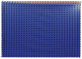
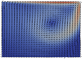
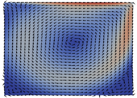
Figure 2: Simulation 1: Arrows and color plot (blue=0.0$-$red=0.75) of the Euclidean norm of the quasi two-dimensional driven cavity flow field along the center plane at three points in time $t=0.8$ and $t=8.0$ and $t=T=80.0$.

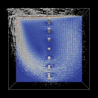
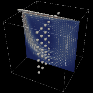
Figure 3: Simulation 2: Arrows and color plot (blue=0.0$-$red=0.75) of the Euclidean norm of the fully three-dimensional driven cavity flow field with obstacles along the center plane at $t=T=24.0$.

In the following, we investigate the performance of the space-time parallel approach for two numerical examples. The first is the classical driven-cavity problem in a quasi-2D setup. Figure 2 shows the flow in a $xy$-plane with $z=0.05$ at times $t=0.8,~{}t=8.0$ and $t=T=80.0$. The second example is an extension where $49$ obstacles (cubes) are inserted into the domain along the median plane, leading to fully 3D flow. Figure 3 sketches the obstacles and the flow at time $t=T=24$. Both problems are posed on a 3D-domain with periodic boundary conditions in $z$-direction (note that $x$ and $z$ are the horizontal coordinates, while $y$ is the vertical coordinate). Initially, velocity and pressure are set to zero. At the upper boundary, a tangential velocity $u_{\rm boundary}=1$ is prescribed, which generates a flow inside the domain as time progresses. No-slip boundary conditions are used at the bottom and in the two $yz$-boundary planes located at $x=0$ and $x=1$ as well as on the obstacles. The parameters for the two simulations are summarized in Table 1. To assess the temporal discretization error of $\mathcal{F}_{\delta t}$, the solution is compared to a reference solution computed with $\mathcal{F}_{\delta t/10}$, giving a maximum error of $1.2\times 10^{-5}$ for the full 3D flow with obstacles. That means that once the iteration of Parareal has reduced the maximum defect between the serial and parallel solution below this threshold, the time-parallel and time-serial solution are of comparable accuracy. We use this threshold also for the quasi-2D example, bearing in mind that the simpler structure of the flow in this case most likely renders the estimate too conservative. The code is run on a Cray XE6 at the Swiss National Supercomputing Centre, featuring a total of 1496 nodes, each with two 16-core 2.1GHz AMD Interlagos CPUs and 32GB memory per node. Nodes are connected by a Gemini 3D torus interconnect and the theoretical peak performance is 402 TFlops.

Table 1: Simulation parameters for the quasi-2D driven cavity flow (Simulation 1) and the fully 3D driven cavity flow with obstacles (Simulation 2).

Sim. 1  :	$\Omega_{h}$  =	$[0,1]\times[0,1]\times[0,0.1]$	Sim. 2  :	$\Omega_{h}$  =	$[0,1]\times[0,1]\times[0,1]$
Sim. 1  :	$N_{x}\times N_{y}\times N_{z}$  =	$32\times 32\times 5$	Sim. 2  :	$N_{x}\times N_{y}\times N_{z}$  =	$32\times 32\times 32$
Sim. 1  :	$T$  =	$80$	Sim. 2  :	$T$  =	$24$
Both  :	$\Delta t$  =	$0.01$	Both  :	$\delta t$  =	$0.001$
Both  :	Re  =	$1000$	Both  :	$u_{\rm boundary}$  =	$1$
Sim. 1  :	$N_{\rm p_{\rm space}}$  =	$1,2,4,8$	Sim. 2  :	$N_{\rm p_{\rm space}}$  =	$1,\ldots,128$
Sim. 1  :	$N_{\rm p_{\rm time}}$  =	$4,8,16$	Sim. 2  :	$N_{\rm p_{\rm time}}$  =	$8,16,32$

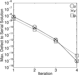
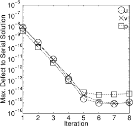
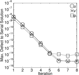
Figure 4: Maximum difference to time-serial solution versus number of Parareal iterations for the Cartesian velocity $(u,v)$ and pressure $p$ of the quasi 2D driven cavity problem at time $t=80.0$ for $N_{p_{\rm time}}=4$ (left), $N_{p_{\rm time}}=8$ (middle) and $N_{p_{\rm time}}=16$ (right).

3.1 Quasi-2D driven cavity flow

Figure 4 shows the maximum difference between the time-parallel and the time-serial solution at the end of the simulation versus the number of iterations of Parareal. In all three cases, the error decreases exponentially with $N_{\rm it}$. The threshold of $1.2\times 10^{-5}$ is reached after a single iteration, indicating that the performance of Parareal could probably be optimized by using a larger $\Delta t$. Figure 5 shows the total speedup provided by the time-serial scheme running $\mathcal{F}_{\delta t}$ with only space-parallelism (circles) as well as by the space-time parallel method for different values of $N_{p_{\rm time}}$. All speedups are measured against the runtime of the time-serial solution run on a single core. The pure spatial parallelization reaches a maximum speedup of a little over 6 using 8 cores. For $N_{\rm it}=1$, the space-time parallel scheme reaches a speedup of 14 using 64 cores. This amounts to a speedup of roughly $14/6\approx 2.33$ from Parareal alone. For $N_{\rm it}=2$ the speedup is down to 8, but still noticeably larger than the saturation point of the pure space-parallel method. Note that because of the limited efficiency of the time parallelization, the slopes of the space-time parallel scheme are lower for larger values of $N_{p_{\rm time}}$.

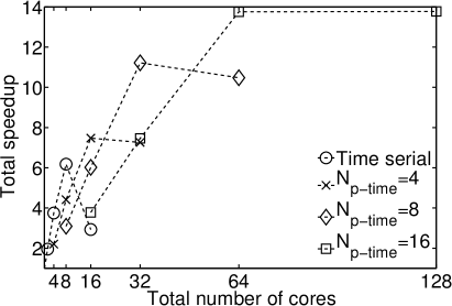
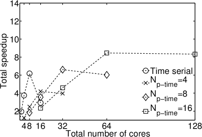
Figure 5: Total speedup of the combined space-time parallelization for quasi 2D driven-cavity flow with $N_{\rm it}=1$ (left) and $N_{\rm it}=2$ (right) iterations.

3.2 Full 3D driven cavity flow with obstacles

Depending on the number of Parareal iterations for three different values of $N_{p_{\rm time}}$ Figure 6 shows the maximum difference between the time-parallel and the time-serial solution in terms of the 3D-Cartesian velocity $(u,v,w)$ and pressure $p$. In general, as in the quasi-2D case, the error decays exponentially with the number of iterations, but now, particularly pronounced for $N_{p_{\rm time}}=32$, a small number of iterations has to be performed without large effect before the error starts to decrease. This is likely due to the increased turbulence caused by the obstacles, as it is known that Parareal exhibits instabilities for advection dominated problems or hyperbolic problems Gander2007 ; RuprechtKrause2012 . A more detailed analysis of the performance of Parareal for turbulent flow and larger Reynolds numbers is left for future work. Figure 7 shows the total speedup measured against the runtime of the solution running $\mathcal{F}_{\delta t}$ serially with $N_{\rm p_{\rm space}}=1$. The time-serial-line (circles) shows the speedup for a pure spatial parallelization, which scales to $N_{\rm p_{\rm space}}=16$ cores and then saturates at a speedup of about 18. Adding time-parallelism can significantly increase the total speedup, to about 20 for $N_{p_{\rm time}}=4$, about 27 for $N_{p_{\rm time}}=8$ and to almost 40 for $N_{p_{\rm time}}=16$ for a fixed number of $N_{\rm it}=3$ iterations (left figure). However, as can be seen from Figure 6, the solution with $N_{\rm p}=32$ is significantly less accurate. The right figure shows the total speedup for a number of iterations adjusted so that the defect of Parareal in all cases is below $10^{-5}$ in all solution components (cf. Figure 6). This illustrates that there is a sweet-spot in the number of concurrently treated time-slices: At some point the potential increase in speedup is offset by the additional iterations required. In the presented example, the solution with $N_{\rm p}=16$ is clearly more efficient than the one with $N_{\rm p}=32$.

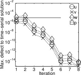
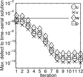
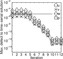
Figure 6: Maximum difference to time-serial solution at end of simulation versus number of Parareal iterations for the 3D driven cavity flow with obstacles for $N_{p_{\rm time}}=8$ (left), $N_{p_{\rm time}}=16$ (middle), $N_{p_{\rm time}}=32$ (right). The horizontal line indicates an error level of $10^{-5}$.

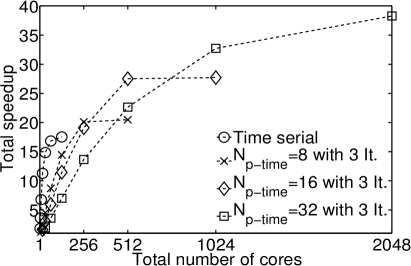
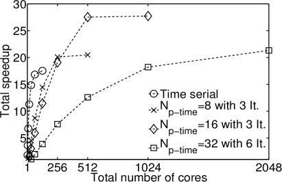
Figure 7: Total speedup of the combined space-time parallelization for 3D cavity flow with obstacles for a fixed number of $N_{\rm it}=3$ iterations (left) and a number of iterations chosen to achieve a defect below $10^{-5}$ in all solution components (right). Note that the solutions in the left figure are not comparable in accuracy.

4 Conclusions

A space-time parallel method, coupling Parareal with spatial domain decomposition, is presented and used to solve the three-dimensional, time-dependent, incompressible Navier-Stokes equations. Two setups are analyzed: A quasi-2D driven cavity example and an extended setup, where obstacles inside the domain lead to a fully 3D driven flow. The convergence of Parareal is investigated and speedups of the space-time parallel approach are compared to speedups from a pure space-parallel scheme. It is found that Parareal converges very rapidly for the quasi-2D case. It also converges in the 3D case, although for larger numbers of Parareal time-slices, convergence starts to stagnate for the first few iterations, likely because of the known stability issues of Parareal for advection dominated flows. Results are reported from runs on up to 128 nodes with a total of 2,048 cores on a Cray XE6, illustrating the feasibility of the approach for state-of-the-art HPC systems. The results clearly demonstrate the potential of time-parallelism as an additional direction of parallelization to provide additional speedup after a pure spatial parallelization reaches saturation. While the limited parallel efficiency of Parareal in its current form is a drawback, we expect the scalability properties of Parareal to direct future research towards modified schemes with relaxed efficiency bounds.

- (1) Chorin, A.J.: Numerical solution of the Navier–Stokes equations. Math. Comput. 22(104), 745–762 (1968)
- (2) Croce, R., Engel, M., Griebel, M., Klitz, M.: NaSt3DGP - a Parallel 3D Flow Solver. URL http://wissrech.ins.uni-bonn.de/research/projects/NaSt3DGP/index.htm
- (3) Emmett, M., Minion, M.L.: Toward an efficient parallel in time method for partial differential equations. Comm. App. Math. and Comp. Sci. 7, 105–132 (2012)
- (4) Farhat, C., Chandesris, M.: Time-decomposed parallel time-integrators: Theory and feasibility studies for fluid, structure, and fluid-structure applications. Int. J. Numer. Methods Engrg. 58, 1397–1434 (2005)
- (5) Fischer, P.F., Hecht, F., Maday, Y.: A parareal in time semi-implicit approximation of the Navier-Stokes equations. In: R. Kornhuber, et al. (eds.) Domain Decomposition Methods in Science and Engineering, LNCSE, vol. 40, pp. 433–440. Springer, Berlin (2005)
- (6) Gander, M.J., Vandewalle, S.: Analysis of the parareal time-parallel time-integration method. SIAM J. Sci. Comp. 29(2), 556–578 (2007)
- (7) Gaskell, P., Lau, A.: Curvature-compensated convective transport: SMART a new boundedness-preserving transport algorithm. Int. J. Numer. Methods Fluids 8, 617–641 (1988)
- (8) Griebel, M., Dornseifer, T., Neunhoeffer, T.: Numerical Simulation in Fluid Dynamics, a Practical Introduction. SIAM, Philadelphia (1998)
- (9) Leonard, B.: A stable and accurate convective modelling procedure based on quadratic upstream interpolation. Comput. Methods Appl. Mech. Eng. 19, 59–98 (1979)
- (10) Lions, J.L., Maday, Y., Turinici, G.: A ”parareal” in time discretization of PDE’s. C. R. Acad. Sci. – Ser. I – Math. 332, 661–668 (2001)
- (11) Minion, M.L.: A hybrid parareal spectral deferred corrections method. Comm. App. Math. and Comp. Sci. 5(2), 265–301 (2010)
- (12) Ruprecht, D., Krause, R.: Explicit parallel-in-time integration of a linear acoustic-advection system. Computers and Fluids 59, 72–83 (2012)
- (13) Temam, R.: Sur l’approximation de la solution des equations de Navier-Stokes par la m´ethode des pas fractionnaires II. Arch. Rational Mech. Anal. 33, 377–385 (1969)
- (14) Trindade, J.M.F., Pereira, J.C.F.: Parallel-in-time simulation of the unsteady Navier-Stokes equations for incompressible flow. Int J. Numer. Meth. Fluids 45, 1123–1136 (2004)
- (15) Trindade, J.M.F., Pereira, J.C.F.: Parallel-in-time simulation of two-dimensional, unsteady, incompressible laminar flows. Num. Heat Trans., Part B 50, 25–40 (2006)
- (16) van der Vorst, H.: Bi–CGStab: A fast and smoothly converging variant of Bi–CG for the solution of nonsymmetric linear systems. SIAM J. Sci. Stat. Comput. 13, 631 (1992)