Fast Inference for Intractable Likelihood Problems using Variational Bayes

Abstract

Variational Bayes (VB) is a popular estimation method for Bayesian inference. However, most existing VB algorithms are restricted to cases where the likelihood is tractable, which precludes their use in many important situations. Tran et al., (2017) extend the scope of application of VB to cases where the likelihood is intractable but can be estimated unbiasedly, and name the method Variational Bayes with Intractable Likelihood (VBIL). This paper presents a version of VBIL, named Variational Bayes with Intractable Log-Likelihood (VBILL), that is useful for cases as Big Data and Big Panel Data models, where unbiased estimators of the gradient of the log-likelihood are available. We demonstrate that such estimators can be easily obtained in many Big Data applications. The proposed method is exact in the sense that, apart from an extra Monte Carlo error which can be controlled, it is able to produce estimators as if the true likelihood, or full-data likelihood, is used. In particular, we develop a computationally efficient approach, based on data subsampling and the MapReduce programming technique, for analyzing massive datasets which cannot fit into the memory of a single desktop PC. We illustrate the method using several simulated datasets and a big real dataset based on the arrival time status of U. S. airlines.

Keywords. Pseudo Marginal Metropolis-Hastings, Big Data, Panel Data, Difference Estimator.

1 Introduction

Given an observed dataset $y$ and a statistical model with a vector of unknown parameters $\theta$, a major aim of statistics is to carry out inference about $\theta$, i.e., estimate the underlying $\theta$ that generated $y$ and assess the associated uncertainty. The likelihood function $p(y|\theta)$, which is the density of the data $y$ conditional on the postulated model and the parameter vector $\theta$, is the basis of Bayesian methods, such as Markov chain Monte Carlo (MCMC) and Variational Bayes (VB). These methods require exact evaluation of the likelihood $p(y|\theta)$ at each value of $\theta$. In many modern statistical applications, however, the likelihood function, and thus the log-likelihood function, is either analytically intractable or computationally intractable, making it difficult to use likelihood-based methods.

An important situation in which the log-likelihood is computationally intractable is Big Data (Bardenet et al.,, 2015; Quiroz et al.,, 2015), where the log-likelihood function, under the independence assumption and without random effects, is a sum of a very large number of terms and thus too expensive to compute. Large panel data models (Fitzmaurice et al.,, 2011) are another example where the log-likelihood is both analytically and computationally intractable as it is a sum of many terms, each being the log of an integral over the random effects and cannot be computed analytically.

There are several methods in the literature that work with an intractable likelihood. A remarkable approach is the pseudo-marginal Metropolis-Hastings (PMMH) algorithm (Andrieu and Roberts,, 2009), which replaces the intractable likelihood in the Metropolis-Hastings ratio by its non-negative unbiased estimator. An attractive property of the PMMH approach is that it is exact in the sense that it is still able to generate samples from the posterior, as if the true likelihood was used. Similarly to standard Metropolis-Hastings algorithms, PMMH is extremely flexible. However, this method is highly sensitive to the variance of the likelihood estimator. The chain might get stuck and mix poorly if the likelihood estimates are highly variable (Flury and Shephard,, 2011). This is because the asymptotic variance of PMMH estimators increases exponentially with the variance of the log of the estimator of the likelihood (Pitt et al.,, 2012), which in turn increases linearly with the sample size. Therefore the PMMH method can be computationally expensive making it unsuitable for Big Data applications.

VB is a computationally efficient alternative to MCMC (Attias,, 1999; Bishop,, 2006). However, most existing VB algorithms are restricted to cases where the likelihood is tractable, which precludes the use of VB in many interesting models. Tran et al., (2017) extend the scope of application of VB to cases where the likelihood is intractable but can be estimated unbiasedly, and name the method Variational Bayes with Intractable Likelihood (VBIL). Their method works with non-negative unbiased estimators of the likelihood, and is useful when it is convenient to obtain unbiased estimates of the likelihood such as in state space models. This paper presents a version of VBIL, called the Variational Bayes with Intractable Log-Likelihood (VBILL), that requires unbiased estimates of the gradient of the log-likelihood. It turns out that, in cases of Big Data both with and without random effects, it is easy and computationally efficient to obtain unbiased estimates of the gradient of the log-likelihood using data subsampling. Consider the case of Big Data without random effects, where the log-likelihood function is a sum of many terms, with each computed analytically. Then the gradient of the log-likelihood is a sum of tractable terms, and this sum can be estimated unbiasedly using data subsampling. In the case of Big Panel Data, each log-likelihood contribution is the log of an intractable integral and thus can no longer be computed analytically. However, we are still able to obtain an unbiased estimate of the gradient of the log-likelihood using subsampling and Fisher’s identity (see Section 2.2). Although data subsampling has now been used in Big Data situations with a very large number of independent observations, we are not aware of any efficient estimation methods for Big Panel Data models. One of the main goals of our paper is to fill this gap.

This paper makes two important improvements to VBIL that greatly enhance its performance. The first is that we take into account the information of the gradient of the log-likelihood, which helps the stochastic optimization procedure more stable and converge faster. The second is that we now aim to minimize the same Kullback-Leibler divergence as that targeted when the likelihood is tractable. That is, VBILL is exact in the sense that, apart from an extra Monte Carlo error which can be controlled, it is able to produce estimators as if the true likelihood or full-data likelihood were used. The VBIL approach of Tran et al., (2017) is exact in this sense only under the condition that the variance of the likelihood estimator is constant.

Our paper also uses the MapReduce programming technique and develops a computationally efficient approach for analyzing massive datasets which do not fit into the memory of a single desktop PC. The implementation of MapReduce uses the divide and combine idea where the data is divided into small chunks, each chunk is processed separately and the chunk-based results are then combined to construct the final estimates. Under some regularity conditions, Battey et al., (2015) show that the information loss due to the divide and combine procedure is asymptotically negligible when the full sample size grows, as long as the number of chunks is not too large. In finite-sample settings, however, the resulting estimators are sensitive to how the data are divided. It is important to note that our final estimator is mathematically justified and independent of the data chunking, as we use the divide and combine procedure mainly to obtain an unbiased estimator of the gradient of log-likelihood for the VBILL algorithm.

The paper is organized as follows. Section 2 describes the VBILL approach and its applications to Big Data problems using data subsampling. Section 3 presents empirical studies and Section 4 concludes. The appendix presents technical details.

2 Variational Bayes with Intractable Log-Likelihood

Let $p(\theta)$ be the prior, $L(\theta):=p(y|\theta)$ the likelihood and $\pi(\theta)\propto p(\theta)L(\theta)$ the posterior distribution of $\theta$. Let $\ell(\theta):=\log L(\theta)$. Our paper, with a small abuse of notation, uses the same notation for the probability distribution and its density function. VB approximates the posterior distribution of $\theta$ by a probability distribution $q_{\lambda}(\theta)$ within some parametric class of distributions such as an exponential family, with parameter $\lambda$ chosen to minimize the Kullback-Leibler divergence between $q_{\lambda}(\theta)$ and $\pi(\theta)$,

$$\text{\rm KL}\left(\lambda\right)=\text{\rm KL}(q_{\lambda}\|\pi):=\int q_{\lambda}(\theta)\log\frac{q_{\lambda}(\theta)}{\pi(\theta)}d\theta.$$

Minimizing this divergence is equivalent to maximizing the lower bound

$$\text{\rm LB}(\lambda)=\int q_{\lambda}(\theta)\log\frac{p(\theta)L(\theta)}{q_{\lambda}(\theta)}d\theta=A(\lambda)+\int q_{\lambda}(\theta)\ell(\theta)d\theta,$$

with $A(\lambda)=\int q_{\lambda}(\theta)\log\frac{p(\theta)}{q_{\lambda}(\theta)}d\theta$. Often $A(\lambda)$ can be computed analytically. Suppose that $\theta\sim q_{\lambda}(\theta)$ can be represented as a deterministic function of a random vector $\epsilon$ whose distribution is independent of $\lambda$. More precisely, let $g(\cdot,\cdot)$ be a function such that $\theta=g(\lambda,\epsilon)\sim q_{\lambda}(\theta)$, where $\epsilon\sim p_{\epsilon}(\epsilon)$ with $p_{\epsilon}(\cdot)$ not dependent on $\lambda$. For example, if $\theta\sim N(\mu,\Sigma)$, then $\theta$ can be written as $\theta=\mu+\Sigma^{1/2}\epsilon$ with $\epsilon\sim N(0,I)$. Hence,

$$\text{\rm LB}(\lambda)=A(\lambda)+{\mathbb{E}}_{\epsilon\sim p_{\epsilon}}[\ell(g(\lambda,\epsilon))].$$

The gradient of the lower bound is

$$\nabla_{\lambda}\text{\rm LB}(\lambda) = \nabla_{\lambda}A(\lambda)+{\mathbb{E}}_{\epsilon\sim p_{\epsilon}}\Big{[}\nabla_{\lambda}g(\lambda,\epsilon)\nabla_{\theta}\ell(g(\lambda,\epsilon))\Big{]}.$$

Note that if $A(\lambda)$ cannot be computed analytically or it is inconvenient to do so, we can always represent the entire $\nabla_{\lambda}\text{\rm LB}(\lambda)$ as an expectation with respect to $\epsilon$. By generating $\epsilon$ from $p_{\epsilon}(\cdot)$, we are able to obtain an unbiased estimator $\widehat{\nabla_{\lambda}\text{\rm LB}}\left(\lambda\right)$ of the gradient $\nabla_{\lambda}\text{\rm LB}\left(\lambda\right)$. Therefore, we can use stochastic optimization to optimize $\text{\rm LB}(\lambda)$. The representation of the gradient $\nabla_{\lambda}\text{\rm LB}(\lambda)$ in terms of an expectation with respect to $\epsilon$ rather than $\theta$ is the so-called reparameterization trick (Kingma and Welling,, 2013). In general it works more efficient than the alternative methods that sample directly from $q_{\lambda}(\theta)$ (Ruiz et al.,, 2016; Tan and Nott,, 2017). One of the reasons is that this reparameterization takes into account the information from the gradient of the log-likelihood.

We now extend the method to the case where $\nabla_{\theta}\ell(\theta)$ is intractable but can be estimated unbiasedly. Let $\widehat{G}(\theta)$ be an unbiased estimator of $\nabla_{\theta}\ell(\theta)$, i.e. ${\mathbb{E}}(\widehat{G}(\theta))=\nabla_{\theta}\ell(\theta)$, where the expectation is with respect to all random variables $u$ needed for computing $\widehat{G}(\theta)=\widehat{G}(\theta,u)$. Typically, $u$ is a set of uniform random numbers. Write $p_{U}(\cdot)$ for the distribution of $u$. Then,

$$\nabla_{\lambda}\text{\rm LB}(\lambda) = \nabla_{\lambda}A(\lambda)+{\mathbb{E}}_{\epsilon\sim p_{\epsilon},u\sim p_{U}}\Big{[}\nabla_{\lambda}g(\lambda,\epsilon)\widehat{G}(\theta,u)\Big{]},\;\;\theta=g(\lambda,\epsilon),$$

which can be estimated unbiasedly by

$$\widehat{\nabla_{\lambda}\text{\rm LB}(\lambda)}=\nabla_{\lambda}A(\lambda)+\frac{1}{S}\sum_{i=1}^{S}\nabla_{\lambda}g(\lambda,\epsilon_{i})\widehat{G}(\theta_{i},u_{i})$$ (1)

where $\epsilon_{i}\sim p_{\epsilon}(\cdot)$, $u_{i}\sim p_{U}(\cdot)$, $\theta_{i}=g(\lambda,\epsilon_{i})$, $i=1,...,S$. Therefore, we can use stochastic optimization (Robbins and Monro,, 1951) to maximize $\text{\rm LB}(\lambda)$ as follows.

Algorithm 1.

• Set the number of samples $S$, initialize $\lambda^{(0)}$ and stop the following iteration if the stopping criterion is met.

• For $t=0,1,...$, compute $\lambda^{(t+1)}=\lambda^{(t)}+a_{t}I_{F}(\lambda^{(t)})^{-1}\widehat{\nabla_{\lambda}LB}\left(\lambda^{\left(t\right)}\right)$.

Here $I_{F}(\lambda)=\text{\rm cov}_{q_{\lambda}}(\nabla_{\lambda}\log q_{\lambda}(\theta))$ is the Fisher information matrix of $\lambda$ w.r.t. $q_{\lambda}(\theta)$. The sequence $\{a_{t},t\geq 0\}$ is the learning rate and should satisfy $a_{t}>0$, $\sum_{t}a_{t}=\infty$ and $\sum_{t}a_{t}^{2}<\infty$ (Robbins and Monro,, 1951).

In Algorithm 1 we use the natural gradient of the lower bound, which is defined as $I_{F}(\lambda)^{-1}{\nabla_{\lambda}\text{\rm LB}}\left(\lambda\right)$. The natural gradient more adequately captures the geometry of the variational distribution $q_{\lambda}$; see, e.g., Amari, (1998). Using this gradient often makes the convergence faster (Tran et al.,, 2017; Hoffman et al.,, 2013). Here, we provide an informal explanation in the current context. It is easy to see that the Hessian matrix of the lower bound is

$$H(\lambda)=\nabla_{\lambda\lambda^{\prime}}[\text{\rm LB}(\lambda)]=\int\nabla_{\lambda\lambda^{\prime}}[\log q_{\lambda}(\theta)]q_{\lambda}(\theta)\log\frac{\pi(\theta)}{q_{\lambda}(\theta)}d\theta-I_{F}(\lambda),$$

which is approximately $-I_{F}(\lambda)$ when $q_{\lambda}\approx\pi$. That is, Algorithm 1 is a Newton-Raphson type algorithm as it uses the second-order information of the target function.

It is important to note that VBILL is exact in the sense that it minimizes the same Kullback-Leibler divergence $\text{\rm KL}(q_{\lambda}\|\pi)$ as the target that we would optimize if the exact likelihood is available. Therefore, apart from an extra Monte Carlo error, the VBILL approach is able to produce estimators as if the true likelihood, or full-data likelihood, was used. The VBIL approach of Tran et al., (2017) works on an augmented space and minimizes a Kullback-Leibler divergence that is equal to $\text{\rm KL}(q_{\lambda}\|\pi)$ only if the variance of the log of the estimated likelihood is constant.

Convergence properties of the stochastic optimization procedure in Algorithm 1 are well-known in the literature (see, e.g., Sacks,, 1958). Similarly to Tran et al., (2017), it is possible to show that the variance of VBILL estimators increases only linearly with the variance of the estimated gradient of the log-likelihood, which suggests that VBILL is robust to variation in estimating this gradient.

Stopping rule

As in Tran et al., (2017), the updating algorithm is stopped if the change in the average value of the lower bounds over a window of $K$ iterations,

$$\overline{\text{\rm LB}}\left(\lambda^{\left(t\right)}\right):=\frac{1}{K}\sum_{k=1}^{K}\widehat{\text{\rm LB}}\left(\lambda^{\left(t-k+1\right)}\right),$$

is less than some threshold $\varepsilon$, where $\widehat{\text{\rm LB}}\left(\lambda\right)$ is an estimate of $\text{\rm LB}\left(\lambda\right)$. Furthermore, we also use the scaled version of the lower bound $\widehat{\text{\rm LB}}\left(\lambda\right)/n$, with $n$ the size of the dataset. The scaled lower bound is roughly independent of the size of the dataset. Our paper sets $K=5$. Alternatively, we can stop the updating algorithm if the change in the average value $\overline{\lambda}^{\left(t\right)}=\left(1/K\right)\sum_{k=1}^{K}\lambda^{\left(t-k+1\right)}$, is less than some threshold $\varepsilon$. A byproduct of using the stopping rule based on the lower bound is that the lower bound estimates can be useful for model selection (Sato,, 2001; Nott et al.,, 2012).

2.1 VBILL with Data Subsampling

This section presents the VBILL method for Big Data. Let $y=\{y_{i},i=1,...,n\}$ be the data set. We assume that the $y_{i}$ are independent so that the likelihood is $L(\theta)=\prod\nolimits_{i=1}^{n}p(y_{i}|\theta)$ and we assume for now that each likelihood contribution $p(y_{i}|\theta)$ can be computed analytically. The log-likelihood is

$$\ell\left(\theta\right):=\sum_{i=1}^{n}\ell_{i}\left(\theta\right),\;\quad\text{where}\quad\ell_{i}\left(\theta\right):=\log p\left(y_{i}|\theta\right).$$ (2)

The gradient of the log-likelihood is

$$\nabla_{\theta}\ell(\theta)=\sum_{i}\nabla_{\theta}\ell_{i}(\theta),$$

where each $\nabla_{\theta}\ell_{i}(\theta)$ can be computed analytically or by using numerical differentiation. We are concerned with the case where this gradient is computationally intractable in the sense that $n$ is so large that computing this sum is impractical. The proposed VBILL approach to this problem is based on the key observation that it is convenient and computationally much cheaper to obtain an unbiased estimator $\widehat{G}(\theta)$ of the gradient of the log-likelihood $\nabla_{\theta}\ell\left(\theta\right)$.

Let $g_{i}(\theta):=\nabla_{\theta}\ell_{i}(\theta)$. Let $\overline{\theta}$ be some central value of $\theta$ obtained by using, for example, Maximum Likelihood or MCMC, based on a representative subset of the full data. By the first-order Taylor series expansion of the vector field $g_{i}(\theta)$ (Apostol,, 1969, Chapter 8),

$$g_{i}(\theta) = g_{i}(\overline{\theta})+\nabla_{\theta^{\prime}}g_{i}(\overline{\theta})(\theta-\overline{\theta})+o(\|\theta-\overline{\theta}\|)$$ (3)

$$= \nabla_{\theta}\ell_{i}(\overline{\theta})+\nabla_{\theta\theta^{\prime}}^{2}\ell_{i}(\overline{\theta})(\theta-\overline{\theta})+o(\|\theta-\overline{\theta}\|)=w_{i}(\theta)+o(\|\theta-\overline{\theta}\|),$$

where

$$w_{i}(\theta):=\nabla_{\theta}\ell_{i}(\overline{\theta})+\nabla_{\theta\theta^{\prime}}^{2}\ell_{i}(\overline{\theta})(\theta-\overline{\theta}),$$

and $o(\delta)$ denotes the small order of $\delta$, meaning $o(\delta)/\delta\to 0$ as $\delta\to 0$. We can write

$$\nabla_{\theta}\ell(\theta) = \sum_{i}w_{i}(\theta)+\sum_{i}d_{i}(\theta)=w(\theta)+d(\theta),$$

with $d_{i}(\theta)=g_{i}(\theta)-w_{i}(\theta)$, $w(\theta)=\sum_{i}w_{i}(\theta)$ and $d(\theta)=\sum_{i}d_{i}(\theta)$. It is computationally cheap to compute the first term

$$w(\theta)=\sum_{i}\nabla_{\theta}\ell_{i}(\overline{\theta})+\Big{(}\sum_{i}\nabla_{\theta\theta^{\prime}}^{2}\ell_{i}(\overline{\theta})\Big{)}(\theta-\overline{\theta})=A(\overline{\theta})+B(\overline{\theta})(\theta-\overline{\theta})$$

because the sums $A(\overline{\theta})$ and $B(\overline{\theta})$ are computed just once. The second term $d(\theta)$ can be estimated unbiasedly by simple random sampling

$$\widehat{d}_{m}(\theta)=\frac{1}{m}\sum_{i=1}^{m}nd_{u_{i}}(\theta),$$

where $u=\left(u_{1},...,u_{m}\right)$, $u_{i}\in F=\{1,2,...,n\}$, is the $m\times 1$ vector of indices obtained by simple random sampling with replacement from the full index set $F$, ${\rm P}(u_{i}=k)=1/n$ for all $k\in F$. Here $m<n$ is the size of subsamples. It is easy to show that ${\mathbb{E}}\left(\widehat{d}_{m}(\theta)\right)=d(\theta)$. Therefore,

$$\widehat{G}\left(\theta,u\right):=w(\theta)+\widehat{d}_{m}(\theta)$$ (4)

is an unbiased estimator of log-likelihood gradient $\nabla_{\theta}\ell(\theta)$.

Since $w_{i}\left(\theta\right)$ is an approximation of $g_{i}\left(\theta\right)$, the differences $d_{i}\left(\theta\right)$ should have roughly the same size across $i$. Thus, $\widehat{d}_{m}(\theta)$ is expected to be an efficient estimator of $d(\theta)$ (Quiroz et al.,, 2015). If $\overline{\theta}$ is an MLE of $\theta$, then by the Bernstein von Mises theorem (see, e.g. Chen,, 1985), $\|\theta-\overline{\theta}\|=O_{P}(n^{-1/2})$, with $O_{P}$ the stochastically big order with respect to the posterior distribution of $\theta$. Then, from (3), the $d_{i}(\theta)$ are very small, and thus $\widehat{G}(\theta,u)$ has a small variance. See also Bardenet et al., (2015) and Quiroz et al., (2015) who demonstrate the efficiency of data subsampling estimators. This guarantees that the variance of the gradient (1) is small, which makes the VBILL procedure highly efficient.

2.2 VBILL with Data Subsampling for Big Panel Data

This section describes the VBILL method for estimating Big Panel Data models. For panel data models with $n$ panels $\left\{y_{1},...,y_{n}\right\}$, also called longitudinal models or generalized linear mixed models, the log-likelihood is still in the form of (2), but each likelihood contribution $p\left({y}_{i}|\theta\right)$ is an integral over random effects $\alpha_{i}$,

$$p\left({y}_{i}|\theta\right)=\int p\left({y}_{i}|\theta,{\alpha}_{i}\right)p\left({\alpha}_{i}|\theta\right)d{\alpha}_{i}.$$ (5)

In many cases the integral (5) is analytically intractable and hence also its first and second derivatives. Therefore, it is intractable to compute the gradients $\nabla_{\theta_{i}}\ell(\theta)$ and $\nabla_{\theta}\ell(\theta)$, even when $n$ is small. However, it is still possible to estimate these gradients unbiasedly.

We first describe how to obtain an unbiased estimator of the gradient of the log-likelihood contributions $\nabla_{\theta}l_{i}\left(\theta\right)$. The gradient $\nabla_{\theta}l_{i}\left(\theta\right)$ can be written as

$$\nabla_{\theta}l_{i}(\theta) = \frac{1}{p(y_{i}|\theta)}\nabla_{\theta}\int p\left({y}_{i},{\alpha}_{i}|\theta\right)d{\alpha}_{i}$$ (6)

$$= \frac{1}{p(y_{i}|\theta)}\int\nabla_{\theta}\log p\left({y}_{i},{\alpha}_{i}|\theta\right)\times p\left({y}_{i},{\alpha}_{i}|\theta\right)d{\alpha}_{i}$$

$$= \int\nabla_{\theta}\log p\left({y}_{i},{\alpha}_{i}|\theta\right)\times p\left({\alpha}_{i}|{y}_{i},\theta\right)d{\alpha}_{i}.$$

The representation in (6) is known in the literature as Fisher’s identity (Cappe et al.,, 2005). Therefore, we can obtain an unbiased estimator of $\nabla_{\theta}l_{i}(\theta)$ by using importance sampling. When $n$ is large, it is clear that we can use the data subsampling approach described in the previous section, together with Fisher’s identity in (6), to obtain an unbiased estimator of the gradient $\nabla_{\theta}\ell(\theta)$.

2.3 Gaussian variational distribution with factor decomposition

Our paper uses a $d$-variate Gaussian distribution ${\cal N}(\theta;\mu,\Sigma)$, with $d$ the number of parameters, for the VB distribution $q_{\lambda}(\theta)$. If necessary, all the parameters can be transformed so that it is appropriate to approximate the posterior of the transformed parameters by a normal distribution. This simplifies the stochastic VB procedure and avoids the factorization assumption in conventional VB that ignores the posterior dependence between the parameter blocks. Using a Gaussian approximation is motivated by the Bernstein von Mises theorem (Chen,, 1985), which states that the posterior of $\theta$ is approximately Gaussian when $n$ is large. Therefore, using a Gaussian variational distribution results in a highly accurate approximation of the posterior distribution.

We also use a factor decomposition for $\Sigma$,

$$\Sigma=BB^{\prime}+c^{2}I_{d},$$ (7)

with $B$ a $d\times 1$-vector, $c$ a scalar and $I_{d}$ the $d\times d$ identity matrix. This factor decomposition helps to reduce the total number of VB parameters from $d+d(d+1)/2$ in the conventional parameterization $\lambda=(\mu,\Sigma)$ to $2d+1$ in the parameterization $\lambda=(\mu,B,c)$. The factorization also helps overcome the problem of obtaining a negative-definite $\Sigma$ if it is updated directly. It is possible to use the factor decomposition (7) where $B$ is a $d\times k$ matrix and $k$ is the number of factors, with $k$ chosen by some model selection criterion (Tan and Nott,, 2017). We use $k=1$ in this paper. Because $B$ is a vector, we are able to find a closed-form expression for the inverse of the Fisher information matrix $I_{F}(\lambda)$ used in Algorithm 1. This closed-form expression leads to a significant gain in computational efficiency in Big Data settings. The closed-form expression for $I_{F}(\lambda)^{-1}$ is in the Appendix.

Initializing $\lambda$

Let $\widehat{\theta}_{n_{\text{sub}}}$ be an estimate of $\theta$ based on a subsample of size $n_{\text{sub}}$ from the full data of size $n$, and let $I_{F,n_{\text{sub}}}$ be the observed Fisher information matrix based on this subsample. We estimate the observed Fisher information matrix based on the full data by $I_{F,n}:=(n/n_{\text{sub}})I_{F,n_{\text{sub}}}$. Let $\widehat{\Sigma}:=I_{F,n}^{-1}$. Motivated by the Bernstein von Mises theorem (see, e.g. Chen,, 1985), which states that the posterior of $\theta$ is approximately Gaussian when $n$ is large, we initialize the VB distribution $q_{\lambda}(\theta)$ by the Gaussian distribution with mean $\widehat{\theta}_{n_{\text{sub}}}$ and covariance matrix $\widehat{\Sigma}$. Let $(\nu_{i},v_{i})$, $\nu_{1}\geq\nu_{2}\geq...$, be the pairs of eigenvalues $\nu_{i}$ with the corresponding eigenvectors $v_{i}$ of $\hat{\Sigma}$. Because $\widehat{\Sigma}=\sum_{i}\nu_{i}v_{i}v_{i}^{\prime}$, we initialize $B$ by $B=\sqrt{\nu_{1}}v_{1}$ and $c$ by $c=[\sum(\text{\rm diag}(\widehat{\Sigma}-BB^{\prime}))/d]^{1/2}$. Then $BB^{\prime}+c^{2}I_{d}\approx\hat{\Sigma}$. The mean $\mu$ is initialized by $\widehat{\theta}_{n_{\text{sub}}}$.

2.4 Randomised Quasi Monte Carlo

Numerical integration using quasi-Monte Carlo (QMC) methods has proved in many cases to be more efficient than standard Monte Carlo methods (Niederreiter,, 1992; Dick and Pillichshammer,, 2010; Glasserman,, 2004). Standard Monte Carlo estimates the integral of interest based on i.i.d points from the uniform distribution ${u}_{s}\sim U\left[0,1\right]^{d}$. QMC chooses these points deterministically and more evenly in the sense that they minimize the so-called star discrepancy of the point set. Randomized QMC (RQMC) then adds randomness to these points such that the resulting points preserve the low-discrepancy property and, at the same time, they have a uniform distribution marginally. Introducing randomness into QMC points is important in order to obtain statistical properties such as unbiasedness and central limit theorems. Our paper generates RQMC numbers using the scrambled net method of Matousek, (1998). We use RQMC to sample $\epsilon\sim p_{\epsilon}\left(\cdot\right)$. For the panel data example, we also use RQMC to obtain unbiased estimates of the likelihood and the gradient of the log-likelihood.

3 Experimental studies

3.1 The US airlines data

We use the airline on-time performance data from the 2009 ASA Data Expo to demonstrate the VBILL methodology. This is a massive dataset that exceeds the memory (RAM) of a single desktop computer. The dataset, used previously by Wang et al., (2015) and Kane et al., (2013) among others, consists of the flight arrival and departure details for all commercial flights within the USA, from October 1987 to April 2008. The full dataset, ignoring the missing values, has 22,347,358 observations.

The response variable of the logistic regression model is late arrival, which is set to 1 if a flight is late by more than 15 minutes and 0 otherwise. There are three covariates. The two binary covariates are: night (1 if the departure occurred at night and 0 otherwise) and weekend (1 if the departure occurred on weekend and 0 otherwise). The third covariate is distance, which is the distance from origin to destination (in 1000 miles).

We first compare the performance of VBILL with data subsampling to MCMC for a subset of $1113638$ observations from the full dataset. This “moderate” data example allows us to run the “gold standard” MCMC, so that we are able to assess the accuracy of VBILL. The MCMC chain, based on the adaptive random walk Metropolis-Hastings algorithm in Haario et al., (2001), consists of 30000 iterates with another 10000 iterates used as burn-in. We also compare the use of RQMC and MC. We use a diffuse normal prior $N\left(0,50I_{4}\right)$ for the coefficient vector $\beta$.

The central value $\overline{\theta}$ is set as the MLE of $\beta$ based on 30% of the full dataset (the one with $1113638$ observations). For the number of samples $S$ in (1), we use $S=2^{8}$ for both MC and RQMC. Choosing $S$ as a power of $2$ (with 2 the base of the Sobol’ sequence in the scrambled net method of Matousek, (1998)) is convenient for the RQMC method. We run this example on a single desktop with 4 local processors. We set the threshold $\varepsilon=10^{-7}$.

Table 1 summarizes the estimation results and, in particular, reports the posterior means and posterior standard deviations of the parameters for the VBILL and MCMC methods. The results for VBILL are obtained by averaging over 100 replications. For VBILL, we use a subsample size $m=10000$ and $20000$, i.e. 1% and 2% of the full dataset. The table shows that the VBILL estimates are very close to the “gold standard” MCMC estimates, but that VBILL is around 20 times faster than MCMC in this moderate data example. The more processors we have, the faster the VBILL method will be. In general, VBILL with RQMC converges with fewer iterations than VBILL with MC. Figures 1 and 2 plot the MCMC and VBILL estimates of the marginal posterior densities of $p\left(\beta|y\right)$. The MCMC density estimates are obtained using the Matlab kernel density function ksdensity. The figures show that the VBILL estimates are very close to the MCMC estimates.

To study the stability of VBILL, Table 2 reports the standard errors, estimated over 100 replications, of the VBILL estimates of the posterior means and posterior standard deviations. Clearly, the standard errors decrease when the subsample size $m$ increases. These standard errors suggest that the VBILL approach in this example is stable in the sense that the VBILL estimates across different runs stay the same up to at least the second decimal place. We can also reduce these standard errors by using a smaller threshold $\varepsilon$.

Table 1: Logistic regression model ($n=1113638$). The table summarizes the estimates of the posterior means and the posterior standard deviations (in brackets). The VBILL results are obtained by averaging over $100$ replications. The CPU time (in minutes) and the number of iterations for VBILL are averaged over the replications.

		MCMC	VBILL
Parameter	$\overline{\theta}$		MC		RQMC
$\beta_{0}$	$-1.598$	$\underset{\left(0.004\right)}{-1.613}$	$\underset{\left(0.004\right)}{-1.609}$	$\underset{\left(0.004\right)}{-1.609}$	$\underset{\left(0.004\right)}{-1.609}$	$\underset{\left(0.004\right)}{-1.609}$
$\beta_{1}$	$-0.175$	$\underset{\left(0.006\right)}{-0.155}$	$\underset{\left(0.004\right)}{-0.158}$	$\underset{\left(0.004\right)}{-0.159}$	$\underset{\left(0.004\right)}{-0.159}$	$\underset{\left(0.004\right)}{-0.159}$
$\beta_{2}$	$0.051$	$\underset{\left(0.004\right)}{0.089}$	$\underset{\left(0.004\right)}{0.086}$	$\underset{\left(0.004\right)}{0.085}$	$\underset{\left(0.004\right)}{0.085}$	$\underset{\left(0.004\right)}{0.085}$
$\beta_{3}$	$0.805$	$\underset{\left(0.007\right)}{0.764}$	$\underset{\left(0.007\right)}{0.766}$	$\underset{\left(0.007\right)}{0.766}$	$\underset{\left(0.007\right)}{0.766}$	$\underset{\left(0.007\right)}{0.767}$
$m$			1%	2%	1%	2%
Iter.		40000	52	29	35	29
CPU time		20.23	1.52	1.03	1.07	0.99

Table 2: Logistic regression model ($n=1113638$). Monte Carlo standard errors of the estimates over 100 replications. The results show that VBILL is stable in the sense that the VBILL estimates across different runs stay the same up to at least the second decimal place.

Parameter	VBILL-MC		VBILL-RQMC
${\mathbb{E}}(\beta_{0}|y)$	$0.0037$	$0.0027$	$0.0035$	$0.0029$
${\mathbb{E}}(\beta_{1}|y)$	$0.0036$	$0.0027$	$0.0034$	$0.0028$
${\mathbb{E}}(\beta_{2}|y)$	$0.0036$	$0.0025$	$0.0033$	$0.0027$
${\mathbb{E}}(\beta_{3}|y)$	$0.0031$	$0.0021$	$0.0028$	$0.0023$
${\mathbb{V}}(\beta_{0}|y)$	$0.2808\times 10^{-5}$	$0.1552\times 10^{-5}$	$0.2103\times 10^{-5}$	$0.1639\times 10^{-5}$
${\mathbb{V}}(\beta_{1}|y)$	$0.2436\times 10^{-5}$	$0.1359\times 10^{-5}$	$0.1816\times 10^{-5}$	$0.1411\times 10^{-5}$
${\mathbb{V}}(\beta_{2}|y)$	$0.2356\times 10^{-5}$	$0.1321\times 10^{-5}$	$0.1771\times 10^{-5}$	$0.1392\times 10^{-5}$
${\mathbb{V}}(\beta_{3}|y)$	$0.6523\times 10^{-5}$	$0.3481\times 10^{-5}$	$0.4756\times 10^{-5}$	$0.3653\times 10^{-5}$
$m$	1%	2%	1%	2%

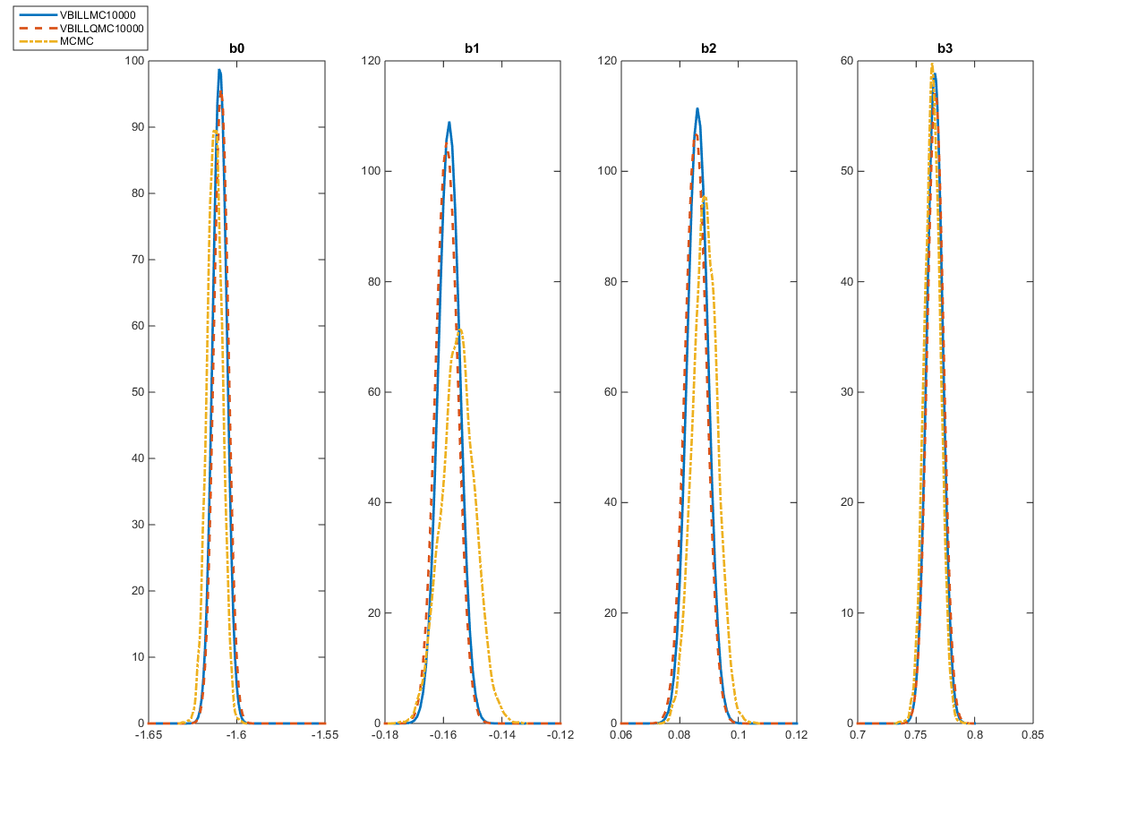
Figure 1: Logistic regression model ($n=1113638,\ m=10000$): Plots of the MCMC and VBILL estimates of the marginal posteriors $p(\beta_{j}|y)$.

Figure 2: Logistic regression model ($n=1113638,\ m=20000$): Plots of the MCMC and VBILL estimates of the marginal posteriors $p(\beta_{j}|y)$.

We now run VBILL for the full dataset, which exceeds the memory of a single desktop computer. Given our computational facilities, it is computationally infeasible to run MCMC to fit the model using such a large dataset. We use the MapReduce programming technique in Matlab to overcome the computer’s memory issue. MapReduce is available in the R2014b release of Matlab. The MapReduce programming model has three components

• A datastore function that reads and organizes the dataset into small chunks for the “map” function.

• A map function calculates the quantities of interest for each individual chunk. MapReduce calls the map function once for each data chunk organized by datastore.

• A reduce function aggregates outputs from the map function and produces the final results.

The datastore function splits the full dataset into $K$ chunks randomly, each fits into the memory of a single desktop computer. The log-likelihood, its gradient and Hessian can be decomposed as

$$\ell\left(\theta\right)=\sum_{k=1}^{K}l^{\left(k\right)}\left(\theta\right),\;\;\;\;\nabla_{\theta}\ell\left(\theta\right)=\sum_{k=1}^{K}\nabla_{\theta}l^{\left(k\right)}\left(\theta\right),\;\;\;\;\nabla_{\theta\theta^{{}^{\prime}}}^{2}\ell\left(\theta\right)=\sum_{k=1}^{K}\nabla_{\theta\theta^{{}^{\prime}}}^{2}l^{\left(k\right)}\left(\theta\right),$$

where $l^{\left(k\right)}\left(\theta\right)$, $\nabla_{\theta}l^{\left(k\right)}\left(\theta\right)$, and $\nabla_{\theta\theta^{{}^{\prime}}}^{2}l^{\left(k\right)}\left(\theta\right)$ are the log-likelihood contribution and its gradient and Hessian based on data chunk $k$. Similarly, we denote by $\widehat{l}_{m_{k}}\left(\theta\right)$ and $\widehat{\nabla_{\theta}l_{m_{k}}\left(\theta\right)}$ the unbiased estimator of $l^{\left(k\right)}\left(\theta\right)$ and $\nabla_{\theta}l^{\left(k\right)}\left(\theta\right)$, based on a random subset of size $m_{k}$ from data chunk $k$. The map function is used to calculate the chunk based estimate $\widehat{l}_{m_{k}}\left(\theta\right)$ and $\widehat{\nabla_{\theta}l_{m_{k}}\left(\theta\right)}$ for each chunk $k$. Then, the reduce function aggregates all the chunk-based unbiased estimates into the full data based estimate of the gradient of the log-likelihood

$$\widehat{G}_{m}\left(\theta\right)=\sum_{k=1}^{K}\widehat{\nabla_{\theta}l_{m_{k}}\left(\theta\right)}.$$ (8)

Then,

$${\mathbb{E}}\left(\widehat{G}_{m}\left(\theta\right)\right)=\sum_{k=1}^{K}{\mathbb{E}}\left(\widehat{\nabla_{\theta}l_{m_{k}}\left(\theta\right)}\right)=\sum_{k=1}^{K}\nabla_{\theta}l^{\left(k\right)}\left(\theta\right)=\nabla_{\theta}l\left(\theta\right).$$

We note that this method is computer-memory efficient in the sense that the full dataset does not need to remain on-hold and can be stored in different places. It is important to note that our VBILL estimator is mathematically justified and independent of data chunking, as the estimator $\widehat{G}_{m}\left(\theta\right)$ in (8) is guaranteed to be unbiased.

The central value $\overline{\theta}$ is the MLE based on 1 million observations of the full dataset and is given in Table 3. We use approximately 5% of the data in each subset. We estimate the gradient of the lower bound using RQMC and set $S=2^{8}$. The VBILL method stopped after 24 iterations and the running time was 77.55 minutes. Table 3 shows the results and Figure 3 shows the marginal posterior density estimates of the parameters, which are bell-shaped with a very small variance as expected with a large dataset. This example demonstrates that the VBILL methodology is useful for Bayesian inference for Big Data.

Table 3: Logistic regression model ($n=22,347,358$). Estimates of the posterior means and the posterior standard deviations (in brackets). The CPU time is in minutes.

Param.	$\overline{\theta}$	VBILL-RQMC
$\beta_{0}$	$-1.613$	$\underset{\left(0.0008\right)}{-1.608}$
$\beta_{1}$	$-0.155$	$\underset{\left(0.0008\right)}{-0.154}$
$\beta_{2}$	$0.088$	$\underset{\left(0.0008\right)}{0.084}$
$\beta_{3}$	$0.764$	$\underset{\left(0.0015\right)}{0.770}$
Iter.		24
CPU time		77.55

Figure 3: Logistic regression model ($n=22,347,358$).

3.2 Simulation Study: Panel Data Model

This section studies the performance of the VBILL method for the panel data model. Data are generated from the following logistic model with a random intercept

$$p\left(y_{it}|\beta,\alpha_{i}\right) = \text{Binomial}\left(1,p_{it}\right),$$

$$\text{logit}\left(p_{it}\right) = x_{it}^{\prime}\beta+\alpha_{i},\;\;\alpha_{i}\sim N\left(0,\tau^{2}\right),$$

for $i=1,...,n$ and $t=1,...,5$. We generate two datasets of $n=1000$ and $n=10000$ with $x_{1,it},...,x_{10,it}\sim U\left(0,1\right)$. Let $\gamma=\log\left(\tau^{2}\right)$, so the model parameters are $\theta=\left(\beta,\gamma\right)$. We use a diffuse normal prior $N\left(0,50I_{d}\right)$ for $\theta$; $d=12$ in this example.

The performance of VBILL is compared to the pseudo-marginal MCMC simulation method (Andrieu and Roberts,, 2009), which is still able to generate samples from the posterior when the likelihood in the Metropolis-Hastings algorithm is replaced by its unbiased estimator. The likelihood in the panel data context is a product of $n$ integrals over the random effects. Each integral is estimated unbiasedly using importance sampling, with the number of importance samples chosen such that the variance of unbiased likelihood estimator is approximately 1 (Pitt et al.,, 2012). Each MCMC chain consists of 30000 iterates with another 10000 used as burn-in iterates.

For VBILL, the central value $\overline{\theta}$ is a simulated maximum likelihood estimate of $\theta$ based on a 30% randomly selected subset of the full dataset. We set $S=2^{8}$ and use both MC and RQMC in VBILL. The number of importance samples used to estimate integrals in (6) is $N=2^{8}$, and $\varepsilon=10^{-5}$. Tables 4 summarizes the performance results for the three methodologies: pseudo-marginal MCMC, VBILL-MC and VBILL-RQMC for various values of subsample size $m$. For VBILL, the results are obtained by averaging over 100 replications. The VBILL estimates are close to the MCMC estimates and they are all close to the true values. However, VBILL is much faster than MCMC. Figures 4, 5, and 6 plot the VBILL and MCMC estimates of the marginal posterior of the parameters. The three figures show that the VBILL marginal posterior estimates are very close to the MCMC estimates for both MC and RQMC and for all subsample sizes. We note that VBILL with RQMC takes longer to run compared to VBILL with MC, with not much difference in the number of iterations and also the resulting marginal posterior estimates in this example. This is because generating RQMC numbers takes a longer time than generating plain pseudo random numbers.

Table 4: Panel data example ($n=1000$): Posterior mean estimates (with posterior standard deviation in brackets). The VBILL results are obtained by averaging over $100$ replications. The CPU time (in minutes) and the number of iterations for VBILL are averaged over 100 replications.

			MCMC	VBILL
Param.	True	$\overline{\theta}$		MC			RQMC
$\beta_{0}$	$-1.5$	$-1.72$	$\underset{\left(0.25\right)}{-1.64}$	$\underset{\left(0.27\right)}{-1.67}$	$\underset{\left(0.27\right)}{-1.67}$	$\underset{\left(0.27\right)}{-1.67}$	$\underset{\left(0.27\right)}{-1.670}$	$\underset{\left(0.26\right)}{-1.67}$	$\underset{\left(0.26\right)}{-1.67}$
$\beta_{1}$	$1.5$	$1.73$	$\underset{\left(0.17\right)}{1.67}$	$\underset{\left(0.13\right)}{1.70}$	$\underset{\left(0.14\right)}{1.70}$	$\underset{\left(0.13\right)}{1.70}$	$\underset{\left(0.13\right)}{1.69}$	$\underset{\left(0.13\right)}{1.69}$	$\underset{\left(0.13\right)}{1.69}$
$\beta_{2}$	$0.5$	$0.22$	$\underset{\left(0.15\right)}{0.16}$	$\underset{\left(0.12\right)}{0.18}$	$\underset{\left(0.12\right)}{0.18}$	$\underset{\left(0.12\right)}{0.18}$	$\underset{\left(0.12\right)}{0.17}$	$\underset{\left(0.12\right)}{0.17}$	$\underset{\left(0.12\right)}{0.17}$
$\beta_{3}$	$0.25$	$0.22$	$\underset{\left(0.16\right)}{0.33}$	$\underset{\left(0.13\right)}{0.29}$	$\underset{\left(0.12\right)}{0.29}$	$\underset{\left(0.12\right)}{0.29}$	$\underset{\left(0.13\right)}{0.32}$	$\underset{\left(0.12\right)}{0.32}$	$\underset{\left(0.12\right)}{0.32}$
$\beta_{4}$	$0.3$	$0.52$	$\underset{\left(0.16\right)}{0.42}$	$\underset{\left(0.13\right)}{0.48}$	$\underset{\left(0.13\right)}{0.48}$	$\underset{\left(0.13\right)}{0.48}$	$\underset{\left(0.13\right)}{0.46}$	$\underset{\left(0.12\right)}{0.46}$	$\underset{\left(0.12\right)}{0.46}$
$\beta_{5}$	$0.8$	$0.69$	$\underset{\left(0.16\right)}{0.78}$	$\underset{\left(0.13\right)}{0.75}$	$\underset{\left(0.13\right)}{0.75}$	$\underset{\left(0.13\right)}{0.75}$	$\underset{\left(0.13\right)}{0.77}$	$\underset{\left(0.13\right)}{0.77}$	$\underset{\left(0.13\right)}{0.77}$
$\beta_{6}$	$0.45$	$0.46$	$\underset{\left(0.15\right)}{0.61}$	$\underset{\left(0.13\right)}{0.55}$	$\underset{\left(0.13\right)}{0.55}$	$\underset{\left(0.13\right)}{0.55}$	$\underset{\left(0.13\right)}{0.59}$	$\underset{\left(0.13\right)}{0.59}$	$\underset{\left(0.12\right)}{0.59}$
$\beta_{7}$	$0.85$	$1.03$	$\underset{\left(0.16\right)}{0.75}$	$\underset{\left(0.13\right)}{0.89}$	$\underset{\left(0.13\right)}{0.89}$	$\underset{\left(0.13\right)}{0.89}$	$\underset{\left(0.13\right)}{0.83}$	$\underset{\left(0.12\right)}{0.82}$	$\underset{\left(0.12\right)}{0.82}$
$\beta_{8}$	$0.75$	$0.46$	$\underset{\left(0.16\right)}{0.58}$	$\underset{\left(0.13\right)}{0.53}$	$\underset{\left(0.13\right)}{0.53}$	$\underset{\left(0.13\right)}{0.53}$	$\underset{\left(0.13\right)}{0.56}$	$\underset{\left(0.13\right)}{0.56}$	$\underset{\left(0.13\right)}{0.56}$
$\beta_{9}$	$0.67$	$1.24$	$\underset{\left(0.15\right)}{0.95}$	$\underset{\left(0.13\right)}{1.09}$	$\underset{\left(0.13\right)}{1.09}$	$\underset{\left(0.13\right)}{1.09}$	$\underset{\left(0.13\right)}{1.02}$	$\underset{\left(0.13\right)}{1.02}$	$\underset{\left(0.13\right)}{1.01}$
$\beta_{10}$	$1.5$	$1.15$	$\underset{\left(0.17\right)}{1.36}$	$\underset{\left(0.13\right)}{1.27}$	$\underset{\left(0.13\right)}{1.27}$	$\underset{\left(0.13\right)}{1.27}$	$\underset{\left(0.13\right)}{1.33}$	$\underset{\left(0.13\right)}{1.33}$	$\underset{\left(0.13\right)}{1.33}$
$\gamma$	$0.41$	$0.60$	$\underset{\left(0.13\right)}{0.41}$	$\underset{\left(0.12\right)}{0.47}$	$\underset{\left(0.12\right)}{0.47}$	$\underset{\left(0.12\right)}{0.47}$	$\underset{\left(0.12\right)}{0.47}$	$\underset{\left(0.12\right)}{0.46}$	$\underset{\left(0.12\right)}{0.46}$
$m$				50	100	200	50	100	200
Iter.			40000	24	22	22	25	26	26
CPU time			80	1.09	1.62	2.86	1.88	3.12	5.40

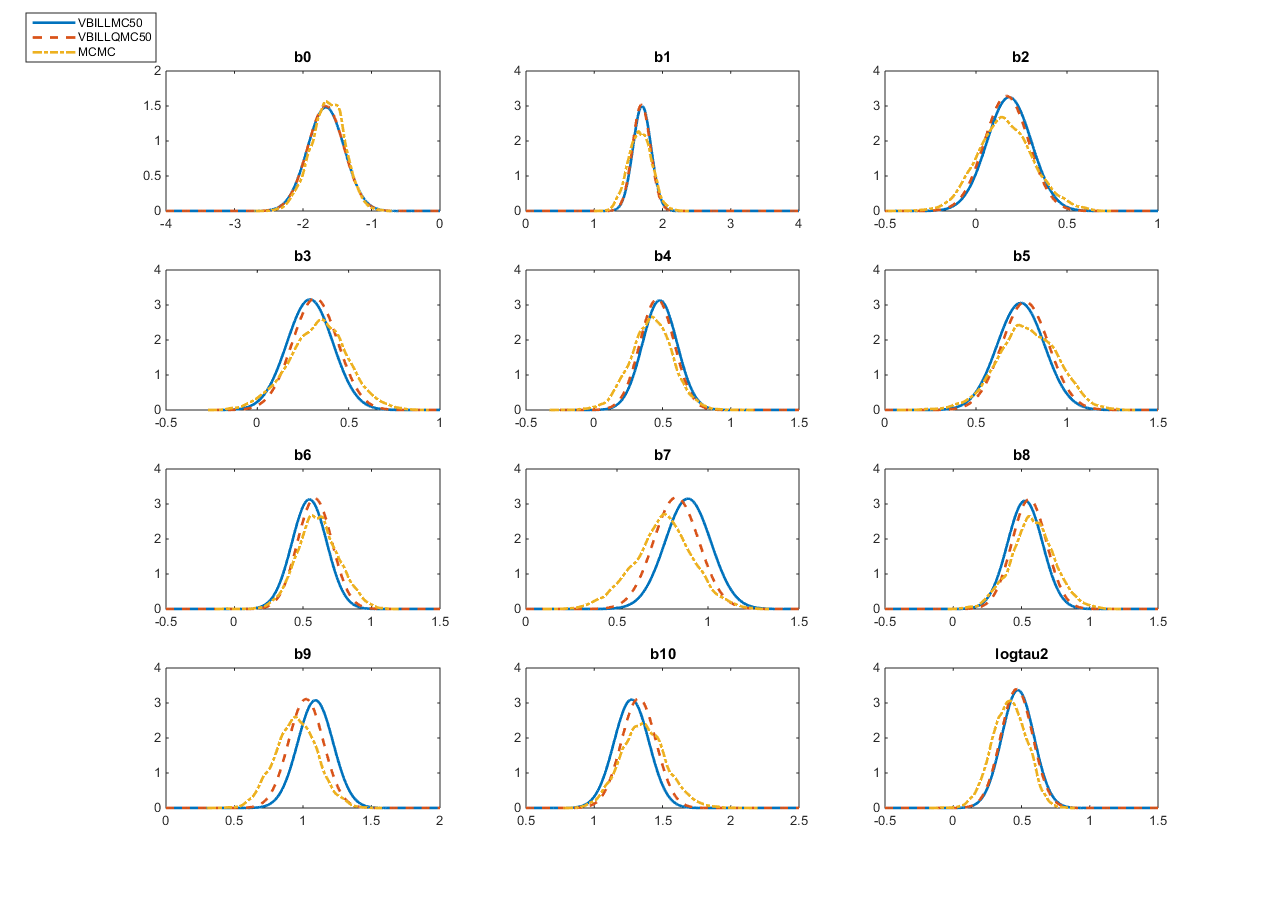
Figure 4: Panel data example ($n=1000$): comparing MCMC and VBILL estimates with $m=50$.

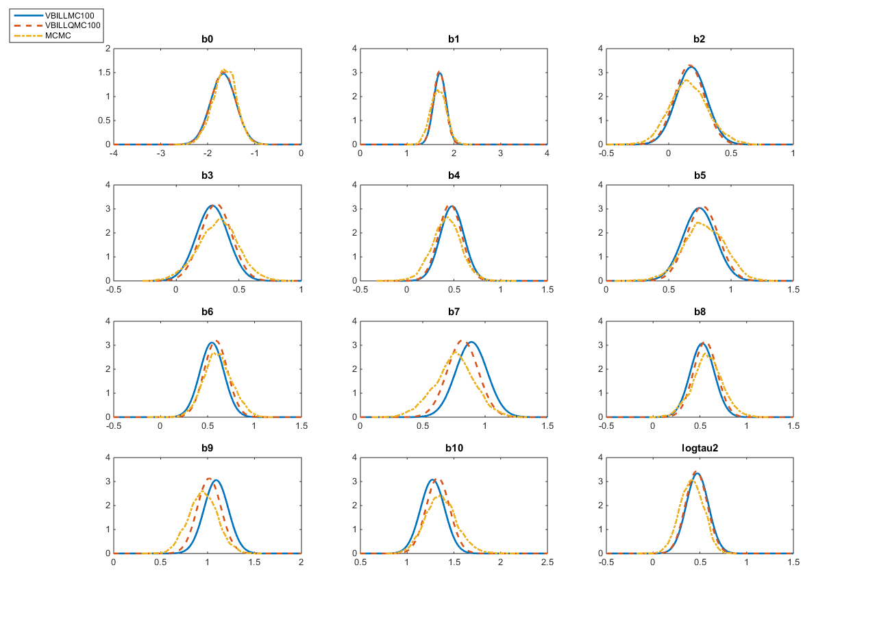
Figure 5: Panel data example ($n=1000$): comparing MCMC and VBILL estimates with $m=100$.

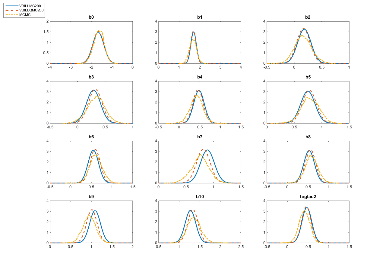
Figure 6: Panel data example ($n=1000$): comparing the MCMC and VBILL estimates with $m=200$.

Larger Panel Data Example

This section describes a scenario where it is difficult to use the pseudo-marginal MCMC method. We consider a large data case with the number of panels $n=10000$. The MCMC method is extremely expensive since the variance of the unbiased estimator of the likelihood is large and it requires approximately $N=8000$ importance samples in order to target the optimal variance of 1 (Pitt et al.,, 2012). Hence, if an optimal MCMC procedure is run on our computer to generate 40000 iterations, it would take $4053.30$ minutes. We run the VBILL-MC and VBILL-RQMC with the subsample size $m=500$ and $\varepsilon=10^{-6}$. Table 5 summarizes the results as averages over 100 replications. Both methods converge on average after 28 and 25 iterations respectively, and result in similar estimates of the posterior mean and standard deviation. The times taken are 8.65 and 13.14 minutes for VBILL-MC and VBILL-RQMC, respectively. The MC errors of the estimates, based on 100 replications, suggest that using RQMC to estimate integrals in (6) helps to stablize the VBILL estimates.

Figure 7 plots the variational approximations of the marginal posteriors of the parameters, which are bell-shaped with small posterior variance as expected with a very large dataset. The two methods produce very similar results. This example demonstrates that VBILL offers a computationally efficient approach for Big Panel Data problems.

Table 5: Panel data example ($n=10000$): The table shows the estimates of posterior mean (first line) and posterior standard deviation (second line). The numbers in brackets are MC standard errors over $100$ replications, which suggests that VBILL-RQMC is more stable than VBILL-MC. The CPU time and number of iterations are averaged over the replications.

Param.	True	$\overline{\theta}$	VBILL-MC	VBILL-RQMC
$\beta_{0}$	$-1.5$	$-1.71$	-1.56 (0.0261)	-1.57 (0.0178)
			0.083 ($0.82\times 10^{-3}$)	0.083 ($0.82\times 10^{-3}$)
$\beta_{1}$	$1.5$	$1.60$	1.54 ($0.0107$)	1.55 ($0.0064$)
			0.041 ($0.30\times 10^{-3}$)	0.042 ($0.25\times 10^{-3}$)
$\beta_{2}$	$0.5$	$0.71$	${0.63}(0.0171)$	${0.63}$ ($0.0133$)
			0.040 ($0.29\times 10^{-3}$)	0.041 ($0.25\times 10^{-3}$)
$\beta_{3}$	$0.25$	$0.24$	${0.20}$ (0.0069)	${0.20}$ (0.0057)
			0.040 ($0.28\times 10^{-3}$)	0.040 ($0.24\times 10^{-3}$)
$\beta_{4}$	$0.3$	$0.34$	${0.32}$ (0.0039)	${0.32}$ (0.0030)
			0.040 ($0.29\times 10^{-3}$)	0.040 ($0.24\times 10^{-3}$)
$\beta_{5}$	$0.8$	$0.69$	${0.70}$ (0.0041)	${0.70}$ (0.0033)
			0.041 ($0.29\times 10^{-3}$)	0.041 ($0.25\times 10^{-3}$)
$\beta_{6}$	$0.45$	$0.56$	${0.51}$ (0.0087)	${0.51}$ (0.0066)
			0.040 ($0.29\times 10^{-3}$)	0.041 ($0.25\times 10^{-3}$)
$\beta_{7}$	$0.85$	$0.80$	${0.79}$ (0.0022)	${0.80}$ (0.0008)
			0.041 ($0.29\times 10^{-3}$)	0.041 ($0.25\times 10^{-3}$)
$\beta_{8}$	$0.75$	$0.79$	${0.76}$ (0.0059)	${0.76}$ (0.0037)
			0.040 ($0.29\times 10^{-3}$)	0.041 ($0.25\times 10^{-3}$)
$\beta_{9}$	$0.67$	$0.70$	${0.69}$ (0.0021)	${0.69}$ (0.0006)
			0.040 ($0.29\times 10^{-3}$)	0.041 ($0.25\times 10^{-3}$)
$\beta_{10}$	$1.5$	$1.56$	${1.56}$ (0.0028)	${1.57}$ (0.0034)
			0.041 ($0.30\times 10^{-3}$)	0.042 ($0.25\times 10^{-3}$)
$\gamma$	$0.41$	$0.35$	$0.36$ (0.0117)	$0.41$ (0.0070)
			0.038 ($0.27\times 10^{-3}$)	0.038 ($0.23\times 10^{-3}$)
$m$			500	500
Iteration			28	25
CPU time (min)			8.65	13.14

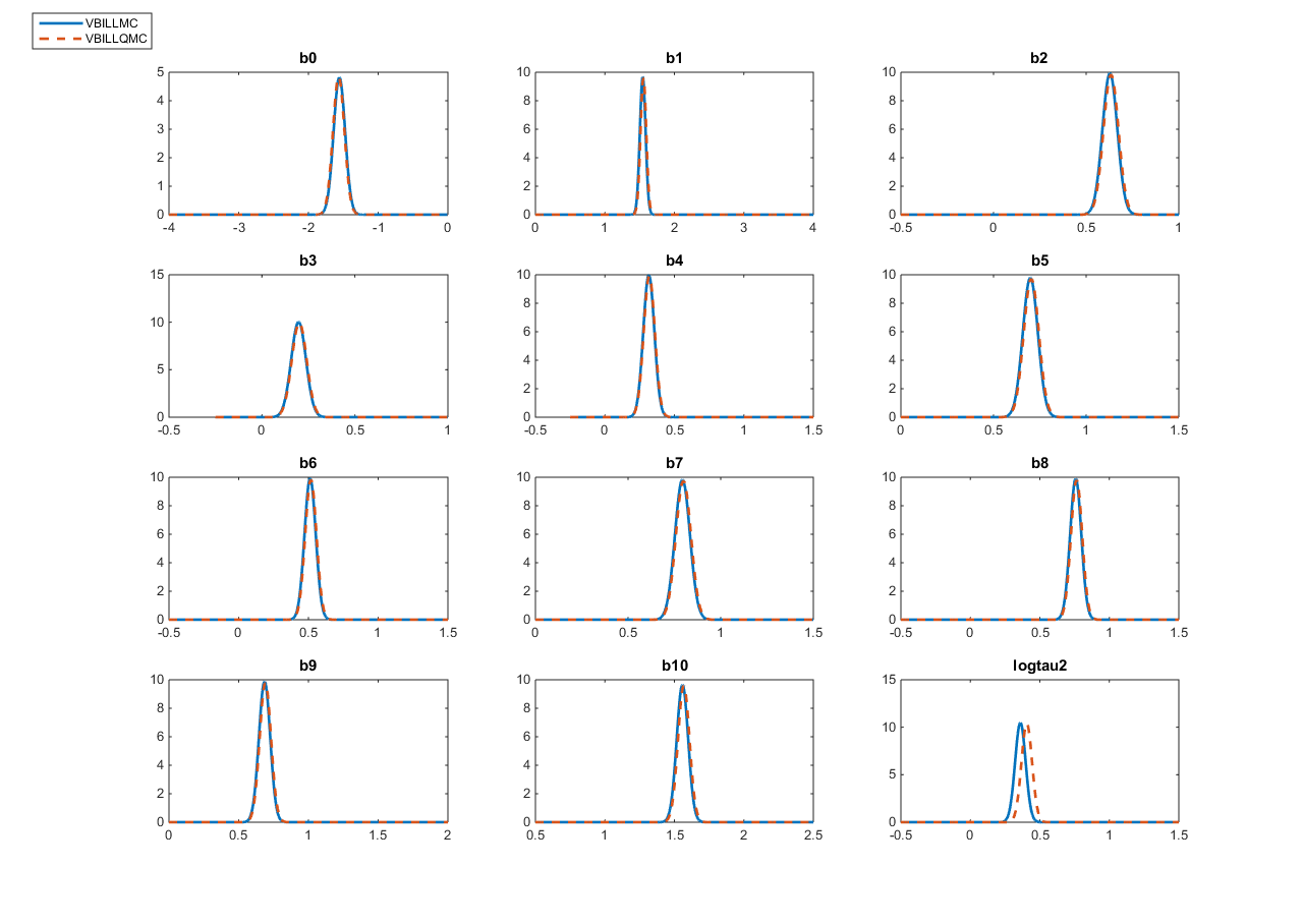
Figure 7: Panel data example ($n=10000$): comparing the MCMC and VBILL estimates with $m=500$

4 Conclusions

We propose the VBILL approach for Bayesian inference when the likelihood function is intractable but the gradient of the log-likelihood can be estimated unbiasedly. The method is useful for Big Data situations where it is convenient to obtain unbiased estimates of the gradient of the log-likelihood.

Unlike MCMC approaches that can in principle sample from the exact posterior, VBILL, as a variant of VB, is an approximate method for estimating the posterior distribution of the parameters. The main advantage of VBILL is that it is much more computationally efficient than MCMC, but produces very similar results to MCMC as shown in the simulated and real examples. To the best of our knowledge, in Big Data situations, there is no MCMC approach in the current literature that is both computationally efficient and able to sample from the exact posterior. Conventional MCMC is exact, but is well-known to be extremely expensive in Big Data, while data subsampling MCMC can be computationally efficient but is not exact (Bardenet et al.,, 2015; Quiroz et al.,, 2015). For these reasons, we believe that VBILL can be the method of choice for Big Data applications.

Appendix

Closed-form expression for $I_{F}(\lambda)^{-1}$

The Fisher information matrix $I_{F}(\lambda)=\text{\rm cov}_{q_{\lambda}}(\nabla_{\lambda}\log q_{\lambda}(\theta))$, where

$$\log q_{\lambda}(\theta)\propto-\frac{1}{2}\log|\Sigma|-\frac{1}{2}(\theta-\mu)^{\prime}\Sigma^{-1}(\theta-\mu),$$

with $\Sigma=BB^{\prime}+c^{2}I_{d}$. Let $U=U(x)$ be a matrix-valued function of a scalar $x$, and $g(U)$ a real-valued function of $U$. Then, by the chain rule (Petersen and Pedersen,, 2012) $\nabla_{x}\big{(}g(U(x))\big{)}=\text{\rm tr}\Big{[}\nabla_{U}\big{(}g(U)\big{)}^{\prime}\nabla_{x}\big{(}U(x)\big{)}\Big{]}.$ Noting that, for vectors $a$ and $b$, $\nabla_{U}(a^{\prime}U^{-1}b)=-U^{-1}ab^{\prime}U^{-1}$ (Petersen and Pedersen,, 2012), we have

$$\nabla_{B}\Big{(}(\theta-\mu)^{\prime}\Sigma^{-1}(\theta-\mu)\Big{)}=-2\Sigma^{-1}(\theta-\mu)(\theta-\mu)^{\prime}\Sigma^{-1}B.$$

$\nabla_{x}(\log|U|)=\text{\rm tr}(U^{-1}\nabla_{x}U)$ because $\nabla_{U}(\log|U|)=U^{-1}$. Hence, $\nabla_{B}\Big{(}\log|\Sigma|\Big{)}=2\Sigma^{-1}B$. Similarly, $\nabla_{c}\Big{(}\log|\Sigma|\Big{)}=2c\times\text{\rm tr}(\Sigma^{-1})$ and $\nabla_{c}\Big{(}(\theta-\mu)^{\prime}\Sigma^{-1}(\theta-\mu)\Big{)}=-2c(\theta-\mu)^{\prime}\Sigma^{-2}(\theta-\mu)$. Hence,

$$\nabla_{\lambda}\log q_{\lambda}(\theta)=\begin{pmatrix}\nabla_{\mu}\log q_{\lambda}(\theta)\\ \nabla_{B}\log q_{\lambda}(\theta)\\ \nabla_{c}\log q_{\lambda}(\theta)\end{pmatrix}=\begin{pmatrix}\Sigma^{-1}(\theta-\mu)\\ -\Sigma^{-1}B+\Sigma^{-1}(\theta-\mu)(\theta-\mu)^{\prime}\Sigma^{-1}B\\ -c\times\text{\rm tr}(\Sigma^{-1})+c(\theta-\mu)^{\prime}\Sigma^{-2}(\theta-\mu)\end{pmatrix}.$$ (9)

Let $X=\Sigma^{-1}(\theta-\mu)\sim{\cal N}(0,\Sigma^{-1})$. Using the results on cubic and quadratic forms of a Gaussian random vector (Petersen and Pedersen,, 2012), it can be shown that

$$I_{F}(\lambda)=\begin{pmatrix}\Sigma^{-1}&O_{d\times d}&O_{d\times 1}\\ O_{d\times d}&\Sigma^{-1}BB^{\prime}\Sigma^{-1}+(B^{\prime}\Sigma^{-1}B)\Sigma^{-1}&2c\Sigma^{-2}B\\ O_{1\times d}&2cB^{\prime}\Sigma^{-2}&2c^{2}\text{\rm tr}(\Sigma^{-2})\end{pmatrix}.$$ (10)

To compute the inverse matrix $I_{F}(\lambda)^{-1}$, we first need some preliminary results. Let $A$ be a $d\times d$ matrix, $b$ a $d\times 1$ vector and $\omega$ a scalar. Then,

$$(A+bb^{\prime})^{-1}=A^{-1}-\frac{1}{1+b^{\prime}A^{-1}b}A^{-1}bb^{\prime}A^{-1}$$

and

$$\begin{pmatrix}A&b\\ b^{\prime}&\omega\end{pmatrix}^{-1}=\begin{pmatrix}A^{-1}+\frac{1}{c_{2}}A^{-1}bb^{\prime}A^{-1}&-\frac{1}{c_{2}}A^{-1}b\\ -\frac{1}{c_{2}}b^{\prime}A^{-1}&\frac{1}{c_{2}}\end{pmatrix},\;\;\;\;\text{ with }\;\;\;\;c_{2}=\omega-b^{\prime}A^{-1}b.$$

Then,

$$\Sigma^{-1}=(BB^{\prime}+c^{2}I)^{-1}=\frac{1}{c^{2}}\left(I-\frac{1}{c^{2}+B^{\prime}B}BB^{\prime}\right),$$

and

$$\Sigma^{-1}B=\alpha B,\;\;\;\;\text{ with }\;\;\;\;\alpha=1/(c^{2}+B^{\prime}B).$$

The Fisher information matrix in (10) can written as

$$I_{F}(\lambda)=\begin{pmatrix}\Sigma^{-1}&O_{d\times d}&O_{d\times 1}\\ O_{d\times d}&A&b\\ O_{1\times d}&b^{\prime}&\omega\end{pmatrix}$$

with

$$A = \Sigma^{-1}BB^{T}\Sigma^{-1}+(B^{T}\Sigma^{-1}B)\Sigma^{-1}=\alpha^{2}BB^{\prime}+\alpha(B^{\prime}B)\Sigma^{-1},$$

$$b = 2c\Sigma^{-2}B=2c\alpha^{2}B=\frac{2c}{(c^{2}+B^{\prime}B)^{2}}B,$$

$$\omega = 2c^{2}\text{\rm tr}(\Sigma^{-2})=\frac{2}{c^{2}}\left[d-1+\left(\frac{c^{2}}{c^{2}+B^{\prime}B}\right)^{2}\right].$$

We have

$$A^{-1}=\left[\left(1+\frac{c^{2}}{B^{\prime}B}\right)-\frac{1}{2}\left(1+\frac{c^{2}}{B^{\prime}B}\right)^{2}\right]BB^{\prime}+c^{2}\left(1+\frac{c^{2}}{B^{\prime}B}\right)I_{d},\;\;\;\;\;\text{and}\;\;\;\;A^{-1}b=\kappa B,$$

with

$$\kappa=\left[\left(1+\frac{c^{2}}{B^{\prime}B}\right)-\frac{1}{2}\left(1+\frac{c^{2}}{B^{\prime}B}\right)^{2}\right]\frac{2c(B^{\prime}B)}{(c^{2}+B^{\prime}B)^{2}}+\frac{2c^{3}}{B^{\prime}B(c^{2}+B^{\prime}B)}.$$

Finally,

$$I_{F}(\lambda)^{-1}=\begin{pmatrix}BB^{\prime}+c^{2}I_{d}&O_{d\times d}&O_{d\times 1}\\ O_{d\times d}&A^{-1}+\frac{\kappa^{2}}{c_{2}}BB^{\prime}&-\frac{\kappa}{c_{2}}B\\ O_{1\times d}&-\frac{\kappa}{c_{2}}B^{\prime}&1/c_{2}\end{pmatrix},$$

with

$$c_{2}=\frac{2}{c^{2}}\left[d-1+\left(\frac{c^{2}}{c^{2}+B^{\prime}B}\right)^{2}\right]-\frac{2c\kappa B^{\prime}B}{(c^{2}+B^{\prime}B)^{2}}.$$

Computing $\nabla_{\lambda}A(\lambda)$

If we use a normal prior $p(\theta)={\cal N}(0,\sigma_{0}^{2}I_{d})$, then

$$A(\lambda) = {\mathbb{E}}_{q_{\lambda}}\left(\log\frac{p(\theta)}{q_{\lambda}(\theta)}\right)$$

$$= -\frac{1}{2\sigma_{0}^{2}}\Big{(}\mu^{\prime}\mu+\text{\rm tr}(BB^{\prime}+c^{2}I)\Big{)}-\frac{1}{2}\log|BB^{\prime}+c^{2}I|+\text{constants}$$

$$= -\frac{1}{2\sigma_{0}^{2}}(\mu^{\prime}\mu+B^{\prime}B+dc^{2})-\frac{1}{2}\log\Big{(}c^{2d}\big{(}1+B^{\prime}B/c^{2}\big{)}\Big{)}+\text{constants}.$$

Hence,

$$\nabla_{\lambda}A(\lambda)=\begin{pmatrix}\nabla_{\mu}A(\lambda)\\ \nabla_{B}A(\lambda)\\ \nabla_{c}A(\lambda)\end{pmatrix}=\begin{pmatrix}-\frac{1}{\sigma_{0}^{2}}\mu\\ -\left(\frac{1}{\sigma_{0}^{2}}+\frac{1}{c^{2}+B^{\prime}B}\right)B\\ -\frac{dc}{\sigma_{0}^{2}}-\frac{1}{c}\left(d-\frac{B^{\prime}B}{c^{2}+B^{\prime}B}\right)\end{pmatrix}.$$

References

• Amari, (1998) Amari, S. (1998). Natural gradient works efficiently in learning. Neural computation, 10(2):251–276.
• Andrieu and Roberts, (2009) Andrieu, C. and Roberts, G. (2009). The pseudo-marginal approach for efficient Monte Carlo computations. The Annals of Statistics, 37:697–725.
• Apostol, (1969) Apostol, T. (1969). Calculus, Vol. 2: Multi-Variable Calculus and Linear Algebra with Applications to Differential Equations and Probability. John Wiley & Sons, 2nd edition.
• Attias, (1999) Attias, H. (1999). Inferring parameters and structure of latent variable models by variational Bayes. In Proceedings of the 15th Conference on Uncertainty in Artificial Intelligence, pages 21–30.
• Bardenet etΒ al., (2015) Bardenet, R., Doucet, A., and Holmes, C. (2015). On Markov chain Monte Carlo methods for tall data. arXiv:1505.02827v1.
• Battey etΒ al., (2015) Battey, H., Fan, J., Liu, H., Lu, J., and Zhu, Z. (2015). Distributed estimation and inference with statistical guarantees. Technical report. arXiv:1509.05457v1.
• Bishop, (2006) Bishop, C.Β M. (2006). Pattern Recognition and Machine Learning. New York: Springer.
• Cappe etΒ al., (2005) Cappe, O., Moulines, E., and Ryden, T. (2005). Inference in Hidden Markov Models. New York: Springer.
• Chen, (1985) Chen, C.-F. (1985). On asymptotic normality of limiting density functions with Bayesian implications. Journal of the Royal Statistical Society. Series B (Methodological), 47(3):540–546.
• Dick and Pillichshammer, (2010) Dick, J. and Pillichshammer, F. (2010). Digital nets and sequence. Discrepancy theory and quasi-Monte Carlo integration. Cambridge University Press, Cambridge.
• Fitzmaurice etΒ al., (2011) Fitzmaurice, G.Β M., Laird, N.Β M., and Ware, J.Β H. (2011). Applied Longitudinal Analysis. John Wiley & Sons, Ltd, New Jersey, 2nd edition.
• Flury and Shephard, (2011) Flury, T. and Shephard, N. (2011). Bayesian inference based only on simulated likelihood: Particle filter analysis of dynamic economic models. Econometric Theory, 1:1–24.
• Glasserman, (2004) Glasserman, P. (2004). Monte Carlo Methods in Financial Engineering. Springer-Verlag, New York.
• Haario etΒ al., (2001) Haario, H., Saksman, E., and Tamminen, J. (2001). An adaptive Metropolis algorithm. Bernoulli, 7:223–242.
• Hoffman etΒ al., (2013) Hoffman, M.Β D., Blei, D.Β M., Wang, C., and Paisley, J. (2013). Stochastic variational inference. Journal of Machine Learning Research, 14:1303–1347.
• Kane etΒ al., (2013) Kane, M.Β J., Emerson, J., and Weston, S. (2013). Scalable strategies for computing with massive data. Journal of Statistical Software, 55 (14):1–19.
• Kingma and Welling, (2013) Kingma, D.Β P. and Welling, M. (2013). Auto-encoding variational bayes. Technical report. https://arxiv.org/abs/1312.6114.
• Matousek, (1998) Matousek, J. (1998). On the L2-discrepancy for anchored boxes. Journal of Complexity, 14:527–556.
• Niederreiter, (1992) Niederreiter, H. (1992). Random Number Generation and Quasi-Monte Carlo Methods. Society for Industrial and Applied Mathematics, Philadelphia.
• Nott etΒ al., (2012) Nott, D.Β J., Tan, S., Villani, M., and Kohn, R. (2012). Regression density estimation with variational methods and stochastic approximation. Journal of Computational and Graphical Statistics, 21:797–820.
• Petersen and Pedersen, (2012) Petersen, K.Β B. and Pedersen, M.Β S. (2012). The matrix cookbook. http://www2.imm.dtu.dk/pubdb/views/edoc_download.php/3274/pdf/imm3274.pdf.
• Pitt etΒ al., (2012) Pitt, M.Β K., Silva, R.Β S., Giordani, P., and Kohn, R. (2012). On some properties of Markov chain Monte Carlo simulation methods based on the particle filter. Journal of Econometrics, 171(2):134–151.
• Quiroz etΒ al., (2015) Quiroz, M., Villani, M., Kohn, R., and Tran, M.-N. (2015). Speeding up MCMC by efficient data subsampling. arXiv preprint arXiv:1404.4178v2.
• Robbins and Monro, (1951) Robbins, H. and Monro, S. (1951). A stochastic approximation method. Annals of Mathematical Statistics, 22:400–407.
• Ruiz etΒ al., (2016) Ruiz, F. J.Β R., Titsias, M.Β K., and Blei, D.Β M. (2016). The generalized reparameterization gradient. Technical report. arXiv:1610.02287v3.
• Sacks, (1958) Sacks, J. (1958). Asymptotic distribution of stochastic approximation procedures. The Annals of Mathematical Statistics, 29(2):373–405.
• Sato, (2001) Sato, M. (2001). Online model selection based on the variational Bayes. Neural Computation, 13(7):1649–1681.
• Tan and Nott, (2017) Tan, L. S.Β L. and Nott, D. (2017). Gaussian variational approximation with sparse precision matrices. Statistics and Computing. To appear.
• Tran etΒ al., (2017) Tran, M.-N., Nott, D., and Kohn, R. (2017). Variational Bayes with intractable likelihood. Journal of Computational and Graphical Statistics. To appear.
• Wang etΒ al., (2015) Wang, C., Chen, M.Β H., Schifano, E., Wu, J., and Yan, J. (2015). A survey of statistical methods and computing for big data. Technical report. arXiv:1502.07989v1.