Numerical calculations on the relative entanglement entropy in critical spin chains

Abstract

We study the relative entanglement entropy (EE) among various primary excited states in two critical spin chains: the $S=1/2$ XXZ chain and the transverse field Ising chain at criticality. For the $S=1/2$ XXZ chain, which corresponds to $c=1$ free boson conformal field theory (CFT), we numerically calculate the relative EE by exact diagonalization and find a perfect agreement with the predictions by the CFT. For the transverse field Ising chain at criticality, which corresponds to the $c=1/2$ Ising CFT, we analytically relate its relative EE to that of the $S=1/2$ XXZ chain and confirm the relation numerically. We also calculate the “sandwiched” Rényi relative EE and again the numerical results agree well with the analytical predictions. Our results are the first direct confirmation of the CFT predictions on the relative EE of the primary excited states in critical spin chains.

1 Introduction

Entanglement entropy quantifies the amount of entanglement of pure states, and is defined by von Neumann entropy of the reduced density matrix. It has been used to study various quantum many-body systems, such as (1+1)-dimensional conformal field theories (CFTs) [1, 2, 3] or (2+1)-dimensional topological phases [4, 5], and also naturally appears in AdS/CFT correspondence [6] which connects a class of large $N$ gauge theories in $d$ dimensions to classical theories of gravity in $(d+1)$-dimensional anti-de Sitter space  [7, 8]. It was also argued that entanglement is strongly related to the spacetime structure itself, dubbed ER=EPR [9].

Relative entropy $S(\rho||\sigma)$ is a useful distance measure between two density matrices $\rho$ and $\sigma$ [10]. It is defined by

$$S(\rho||\sigma)={\rm tr}\left(\rho\log\rho\right)-{\rm tr}\left(\rho\log\sigma\right),$$ (1)

and has several nice properties [11]. First of all, this quantity is positive definite and becomes zero only when $\rho=\sigma$. Second, when we consider reduced density matrices of some region $A$ in a quantum field theory, although their von Neumann entropies suffer from the ultraviolet divergence coming from short-distance entanglement, the relative entropy between them is finite and therefore remains to be well-defined. Furthermore the relative entropy is free from the ambiguity of the choice of the operator algebra of the region in question [12]. Third, it satisfies the monotonicity property: when the region $A$ is included in the region $B$, $A\subset B$, the relative entropy of the region $B$ is larger than that of the region $A$, $S(\rho_{A}||\sigma_{A})\leq S(\rho_{B}||\sigma_{B})$, where $\rho_{A(B)},\sigma_{A(B)}$ are the reduced density matrices of the states $\rho,\sigma$ for the region $A(B)$. These properties play a crucial role in the recent development of information theoretic approach to quantum field theories, see for example [13, 14, 15, 16, 17].

It is nevertheless often difficult to compute relative entropy between two reduced density matrices in quantum field theories. In [19] a replica trick to calculate the relative entropy was introduced. Based on this trick, a general formula for the relative entropy between two arbitrary reduced density matrices of small subsystems in (1+1)-dimensional CFT was derived [20]. The result was later generalized to higher-dimensional CFT [21, 22] and the case of two disjoint subsystems [23]. When one of the reduced density matrices is coming from the vacuum, one can compare these results with the holographic ones derived from the holographic entanglement entropy formula  [7, 8], and the calculations in the gravity side completely agree with the CFT results [21].  Also, in [27] the dynamics of the relative entropy between the locally excited states and the ground state in (1+1)-dimensional CFT was calculated.

In [28] Ruggiero and Calabrese studied the Rényi relative entropy,

$$S_{n}(\rho||\sigma)=\frac{1}{1-n}\log\left(\frac{\tr\rho\sigma^{n-1}}{\tr\rho^{n}}\right),\>\>\lim_{n\to 1}S_{n}(\rho||\sigma)=S(\rho\|\sigma),$$ (2)

between several excited states in the XX spin chain model and compared the results with the CFT predictions. They used the formula which relates the correlation matrix of the system to the Rényi relative entropy $S_{n}$ in numerical calculations, and the numerical results match the CFT predictions well. This method, however, is only applicable to free (quadratic) systems and it is difficult to take the limit $n\rightarrow 1$, or calculate the relative entropy itself. In addition, the definition of the Rényi relative entropy (2) is different from the one conventionally used in the field of quantum information theory, and its meaning from the viewpoint of quantum information theory has not been obvious yet.

In this paper we perform a numerical study of the relative entropy itself rather than the Rényi counterpart of it in critical spin chain models. In particular, we consider the $S=1/2$ XXZ chain and the critical transverse field Ising chain under the periodic boundary condition. We utilize exact diagonalization to explicitly construct reduced density matrices of excited states of the models and calculate relative entropies among them. The numerical results show a perfect agreement with the analytical results of the corresponding CFTs ($c=1$ free boson CFT for the XXZ chain and the $c=1/2$ Ising CFT for the critical transverse field Ising chain). Moreover, by taking advantage of exact diagonalization, we also calculate the “sandwiched” Rényi relative entropy [29, 30, 31, 32] of the order of $\alpha=1/2$, or quantum fidelity, between excited eigenstates of the XXZ chain. The numerical results again match the CFT predictions in [29].

This paper is organized as follows. In section 2 we explain our setup and how to compute the relative entropy by using the replica trick [19] in two-dimensional CFT. In section 3 we review the previous results of the relative entropy in $c=1$ CFT [19, 28]. The sections 4 and 5 consist of our new results. In section 4 we derive analytic expressions of the relative entropy between several primary excited states in the $c=1/2$ Ising CFT. In section 5 we present extensive numerical results on the relative entropy in critical spin chains. In section 6, we conclude our study and discuss future work.

2 Basic definitions

2.1 Setup

We start from a two-dimensional CFT on a cylinder $\mathbb{R}_{t}\times S^{1}$ with the coordinates $(t,\phi),\phi\sim\phi+2\pi$. We choose our subsystem $A$ to be the segment $\{\phi|-\pi x<\phi<\pi x\}$ at $t=0\>\>(0<x<1)$, and consider the reduced density matrix $\rho_{V}$ of an excited state $|V\rangle$,

$$\rho_{V}={\rm tr}_{A_{c}}|V\rangle\langle V|,$$ (3)

where $A_{c}$ denotes the complement of the region $A$.

The quantity ${\rm tr}\rho_{V}^{n}$ can be calculated by a path integral on the $n$-sheet cylinder with the cut along the subsystem $A$ and the boundary conditions at $t=\pm\infty$ specifying the excited state $|V\rangle$. Furthermore, by applying a uniformarization map and using the state-operator correspondence, we see that the path integral is proportional to the $2n$ point function on the cylinder [33, 34],

$$F^{n}_{V}(x)\equiv\frac{{\rm tr}\rho_{V}^{n}}{{\rm tr}\rho_{(0)}^{n}}=\left(\frac{1}{n}\right)^{2n\Delta_{V}}\frac{\tilde{F}^{n}_{V}(x)}{\langle V(t_{0,1})V^{\dagger}(t^{\prime}_{0,1})\rangle^{n}},\quad\tilde{F}^{n}_{V}(x)\equiv\langle\prod^{n-1}_{k=0}V(t_{k,n})V^{\dagger}(t^{\prime}_{k,n})\rangle$$ (4)

where $\frac{1}{1-n}\log\left({\rm tr}\rho_{(0)}^{n}\right)$ is the $n$-th Rényi entanglement entropy of the vacuum, the $V(z)$ is the local operator corresponding to the excited state $\ket{V}$ with the conformal dimensions $(h_{V},\bar{h}_{V}),\;\Delta_{V}=h_{V}+\bar{h}_{V}$, and $(t_{k,n},t^{\prime}_{k,n})$ are given by

$$t_{k,n}=\frac{\pi}{n}(x+2k),\quad t^{\prime}_{k,n}=\frac{\pi}{n}(-x+2k).$$ (5)

Also, $V^{\dagger}(z)$ denotes the Belavin-Polyakov-Zamolodchikov conjugate of $V$.

2.2 Replica tricks for relative entropy

To compute the relative entropy $S(\rho||\sigma)$ between two density matrices $\rho$ and $\sigma$, it is useful to introduce the following replica trick,

$$\log G_{n}(\rho||\sigma)=\log\tr\rho^{n}-\log\tr\rho\sigma^{n-1},$$ (6)

which recovers the relative entropy in the limit of $n\rightarrow 1$,

$$S(\rho||\sigma)=\lim_{n\rightarrow 1}\frac{1}{n-1}\log G_{n}(\rho||\sigma).$$ (7)

We are interested in the case where $\rho$ and $\sigma$ are reduced density matrices of excited states $|V\rangle,|W\rangle$, $\rho=\rho_{V},\;\sigma=\rho_{W}\equiv{\rm tr}_{A_{c}}|W\rangle\langle W|$. In this setup the second term of (6) also can be written in terms of the correlation function of $V$ and $W$,

$$F^{1,n-1}_{V,W}(x) \equiv \frac{{\rm tr}\rho_{V}\rho_{W}^{n-1}}{{\rm tr}\rho_{(0)}^{n}}$$ (8)

$$= \left(\frac{1}{n}\right)^{2\Delta_{V}+2(n-1)\Delta_{W}}\frac{\tilde{F}^{1,n-1}_{V,W}(x)}{\langle V(t_{0,1})V^{\dagger}(t^{\prime}_{0,1})\rangle\langle W(t_{0,1})W^{\dagger}(t^{\prime}_{0,1})\rangle^{n-1}}$$

with

$$\tilde{F}^{1,n-1}_{V,W}(x)\equiv\langle V(t_{0,n})V^{\dagger}(t^{\prime}_{0,n})\prod^{n-1}_{k=1}W(t_{k,n})W^{\dagger}(t^{\prime}_{k,n})\rangle$$ (9)

where $\Delta_{W}$ is the scaling dimension of the operator $W$. In terms of these quantities the relative entropy between two reduced density matrices $\rho_{V},\rho_{W}$ is given by

$$\log G_{n}(\rho_{V}||\rho_{W})=\log F^{n}_{V}(x)-\log F^{1,n-1}_{V,W}(x),$$ (10)

and (7).

Another replica trick known in the literature is the sandwiched Rényi relative entropy [32, 29] defined by

$$\hat{S}_{\alpha}(\rho||\sigma)=\frac{1}{\alpha-1}\log{\rm tr}(\rho_{\alpha})^{\alpha},\qquad\rho_{\alpha}=\sigma^{\frac{1-\alpha}{2\alpha}}\rho\sigma^{\frac{1-\alpha}{2\alpha}}.$$ (11)

In the limit of $\alpha\rightarrow 1$, (11) yields the relative entropy (1). The sandwiched Rényi relative entropy has several nice properties from the viewpoint of quantum information theory such as monotonicity under completely positive, trace-preserving maps  [32]. Also when $\alpha=1/2$, this is related to another measure of distance of density matrices called quantum fidelity $F(\rho||\sigma)$  [35],

$$F(\rho||\sigma)\equiv{\rm tr}\sqrt{\sqrt{\sigma}\rho\sqrt{\sigma}}=\exp\left[-\frac{1}{2}\hat{S}_{\frac{1}{2}}(\rho||\sigma)\right].$$ (12)

3 Relative entropy in $c=1$ CFT

In this section we discuss relative entropy in $c=1$ CFT. The results in this section have already derived in [28] , thus the purpose of this section is briefly summarizing them for the comparisons with numerical results in the later sections.

$c=1$ CFT is the theory of a free real boson. The action is given by

$$S=\frac{g}{8\pi}\int dz^{2}\partial\varphi\bar{\partial}\varphi.$$ (13)

For the later purpose it is convenient to introduce chiral and anti-chiral fields $\phi(z),\bar{\phi}(\bar{z}),\;\varphi=\phi(z)-\bar{\phi}(\bar{z})$. There are two primary operators of interest in the theory. The first one is the (non-chiral) vertex operator defined by

$$V_{\alpha,\alpha}(z,\bar{z})=:e^{i\alpha(\phi(z)+\bar{\phi}(\bar{z}))}:,$$ (14)

and its conformal dimensions are

$$\left(h_{\alpha},\bar{h}_{\alpha}\right)=\left(\frac{\alpha^{2}}{2g},\;\frac{\alpha^{2}}{2g}\right).$$ (15)

The second one is the current operator $i\partial\phi$ whose conformal dimensions are

$$\left(h_{i\partial\phi},\;\bar{h}_{i\partial\phi}\right)=\left(1,0\right).$$ (16)

3.1 $S(\rho_{V_{\alpha,\alpha}}||\rho_{GS})$

Let us begin with the relative entropy $S(\rho_{V_{\alpha,\alpha}}||\rho_{GS})$ between the reduced density matrix $\rho_{V_{\alpha,\alpha}}$ of the vertex operator $V_{\alpha,\alpha}$ and that of the ground state, $\rho_{GS}$. Now (10) is given by

$$\log G_{n}(\rho_{V_{\alpha,\alpha}}||\rho_{GS})=\log F^{n}_{V_{\alpha,\alpha}}(x)-\log F^{1,n-1}_{V_{\alpha,\alpha},1}.$$ (17)

It was shown in [33, 34] that the first term is independent of $x$, $F^{n}_{V_{\alpha,\alpha}}(x)=1$. The second term is universal (fixed solely by conformal symmetry),

$$F^{1,n-1}_{V_{\alpha,\alpha},1}=\left(\frac{1}{n}\right)^{2\Delta_{\alpha}}\frac{\langle V_{\alpha,\alpha}(t_{0,n})V^{\dagger}_{\alpha,\alpha}(t^{\prime}_{0,n})\rangle}{\langle V_{\alpha,\alpha}(t_{0,1})V^{\dagger}_{\alpha,\alpha}(t^{\prime}_{0,1})\rangle}=\left(\frac{\sin\pi x}{n\sin\frac{\pi x}{n}}\right)^{2\Delta_{\alpha}},\quad\Delta_{\alpha}=h_{\alpha}+\bar{h}_{\alpha}.$$ (18)

From these expressions we reach

$$S(\rho_{V_{\alpha,\alpha}}||\rho_{GS})=2\Delta_{\alpha}(1-\pi x\cot\pi x).$$ (19)

Also, the argument here makes it clear that for any state $V$ with vanishing Rényi entropy $F^{n}_{V}(x)=1$, the relative entropy is given by

$$S(\rho_{V}||\rho_{GS})=2\Delta_{V}(1-\pi x\cot\pi x),$$ (20)

where $\Delta_{V}$ is the scaling dimension of the state.

3.2 $S(\rho_{i\partial\phi}||\rho_{GS})$

Next we consider the relative entropy $S(\rho_{i\partial\phi}||\rho_{GS})$ between the reduced density matrix $\rho_{i\partial\phi}$ of the current operator and $\rho_{GS}$. In this case, the first term of (10) is non-trivial,

$$F^{n}_{i\partial\phi}(x)=\left(\frac{1}{n}\right)^{2}\frac{\langle\prod^{n-1}_{k=0}i\partial\phi(t_{k,n})i\partial\phi(t^{\prime}_{k,n})\rangle}{\langle i\partial\phi(t_{0,1})i\partial\phi(t^{\prime}_{0,1})\rangle^{n}}=\frac{1}{n^{2}\left[4\langle i\partial\phi(t_{0,1})i\partial\phi(t^{\prime}_{0,1})\rangle\right]^{n}}{\rm det}\left[\frac{1}{\sin\frac{t_{ij}}{2}}\right]_{i,j\in[1,2n]}.$$ (21)

$t_{ij}$ in the right-hand side is defined by

$$t_{2k+1}=t_{k,n},\quad t_{2k+2}=t^{\prime}_{k,n},\quad t_{ij}=t_{i}-t_{j}.$$ (22)

The analytic continuation of the determinant was worked out in [36, 37], and the result is

$${\rm det}\left[\frac{1}{\sin\frac{t_{ij}}{2}}\right]_{i,j\in[1,2n]}=4^{n}\frac{\Gamma^{2}(\frac{1+n+n\csc\pi x}{2})}{\Gamma^{2}(\frac{1-n+n\csc\pi x}{2})}.$$ (23)

The second term of the replica (10) in this case is again universal as in (18), and by taking $n\rightarrow 1$ limit, we obtain

$$S(\rho_{i\partial\phi}||\rho_{GS})=2\left(\log(2\sin\pi x)+1-\pi x\cot\pi x+\psi_{0}\left(\frac{\csc\pi x}{2}\right)+\sin\pi x\right),$$ (24)

where $\psi_{0}(x)$ is the digamma function.

3.3 $S(\rho_{i\partial\phi}||\rho_{V_{\alpha,\alpha}})$

Here we consider the relative entropy $S(\rho_{i\partial\phi}||\rho_{V_{\alpha,\alpha}})$ between the current operator and the vertex operator. The first term of (10) has already computed in the previous subsection. The second term is given by

$$\tilde{F}^{1,n-1}_{i\partial\phi,V_{\alpha,\alpha}}(x)=\langle i\partial\phi(t_{0,n})i\partial\phi(t^{\prime}_{0,n})\prod^{n-1}_{k=1}V_{\alpha,\alpha}(t_{k,n})V^{\dagger}_{\alpha,\alpha}(t^{\prime}_{k,n})\rangle.$$ (25)

It was argued [28] that in the limit of $n\rightarrow 1$ this correlator effectively gets factorized

$$\tilde{F}^{1,n-1}_{i\partial\phi,V_{\alpha,\alpha}}(x) = \langle i\partial\phi(t_{0,n})i\partial\phi(t^{\prime}_{0,n})\rangle\langle\prod^{n-1}_{k=1}V_{\alpha,\alpha}(t_{k,n})V^{\dagger}_{\alpha,\alpha}(t^{\prime}_{k,n})\rangle+O((n-1)^{2})$$ (26)

$$= \tilde{F}^{1,n-1}_{i\partial\phi,1}(x)\tilde{F}^{1,n-1}_{1,V_{\alpha,\alpha}}(x)+O((n-1)^{2}),$$

and with the definitions of $F^{n}_{V}(x),F^{1,n-1}_{V,W}(x)$ (4, 8), we have

$$\log G_{n}(\rho_{i\partial\phi}||\rho_{V_{\alpha,\alpha}}) = \log F^{n}_{i\partial\phi}(x)-\log F^{1,n-1}_{i\partial\phi,V_{\alpha,\alpha}}(x)$$ (27)

$$= \log G_{n}(\rho_{i\partial\phi}||\rho_{GS})+\log G_{n}(\rho_{GS}||\rho_{V_{\alpha,\alpha}}),\quad n\rightarrow 1.$$

Therefore the relative entropy $S(\rho_{i\partial\phi}||\rho_{V_{\alpha,\alpha}})$ is given by the sum of the two relative entropies,

$$S(\rho_{i\partial\phi}||\rho_{V_{\alpha,\alpha}})=S(\rho_{i\partial\phi}||\rho_{GS})+S(\rho_{GS}||\rho_{V_{\alpha,\alpha}}).$$ (28)

4 Relative entropy in $c=1/2$ CFT

In this section we consider the relative entropy in the $c=1/2$ Ising CFT and show analytical results of it for the first time. We also reveal the relationship between the relative entropies in $c=1$ free boson CFT and the $c=1/2$ Ising CFT.

$c=1/2$ Ising CFT is the theory of a free Majorana fermion. The action is given by

$$S=\frac{1}{8\pi}\int dz^{2}\left[\psi\partial\psi+\bar{\psi}\bar{\partial}\bar{\psi}\right].$$ (29)

In the discussion below, we focus on two primary operators in this theory, namely the spin operator $\sigma$ and the energy operator $\varepsilon$. The conformal dimensions of them are

$$\left(h_{\sigma},\bar{h}_{\sigma}\right)=\left(\frac{1}{16},\frac{1}{16}\right),\quad\left(h_{\varepsilon},\bar{h}_{\varepsilon}\right)=\left(\frac{1}{2},\frac{1}{2}\right).$$ (30)

It is useful to introduce the bosonization technique to calculate correlation functions of these operators. Let us consider two copies of the $c=1/2$ Ising CFT, i.e., the theory of two decoupled Majorana fermions $\psi_{1},\psi_{2}$. One can form a Dirac fermion $D(z)$ from them [38],

$$D(z)=\frac{1}{\sqrt{2}}\left(\psi_{1}+i\psi_{2}\right),\quad\bar{D}(\bar{z})=\frac{1}{\sqrt{2}}\left(\bar{\psi}_{1}+i\bar{\psi}_{2}\right).$$ (31)

The Dirac fermion can be bosonized,

$$D(z)=e^{i\phi(z)},\quad\bar{D}(\bar{z})=e^{i\bar{\phi}(\bar{z})},$$ (32)

where $\phi,\bar{\phi}$ consist of holomorphic and anti-holomorphic part of the boson field $\varphi$, $\varphi(z,\bar{z})\equiv\phi(z)-\bar{\phi}(\bar{z})$. This boson field $\varphi$ is related to products of the primary operators in two copies of the Ising CFT, such as

$$\varepsilon_{1}=i\psi_{1}\bar{\psi}_{1},\>\varepsilon_{2}=i\psi_{2}\bar{\psi}_{2}\;\rightarrow\;\varepsilon_{1}\varepsilon_{2}=\partial\varphi\bar{\partial}\varphi,$$ (33)

and

$$\sigma_{1}\sigma_{2}=\sqrt{2}\cos\frac{\varphi}{2}.$$ (34)

We will use these properties in calculations of the relative entropies in the Ising CFT.

4.1 $S(\rho_{\sigma}||\rho_{GS})$

Let us consider the relative entropy between the spin operator $\sigma$ and the ground state. The replica trick (10) is now

$$\log G_{n}(\rho_{\sigma}||\rho_{GS})=\log F^{n}_{\sigma}(x)-\log F^{1,n-1}_{\sigma,1}(x).$$ (35)

The first term can be computed by the bosonization explained in the previous subsection [33, 34]

$$\langle\prod^{n-1}_{k=0}\sigma(t_{k,n})\sigma(t^{\prime}_{k,n})\rangle^{2} = \langle\prod^{n-1}_{k=0}\sigma_{1}(t_{k,n})\sigma_{2}(t_{k,n})\sigma_{1}(t^{\prime}_{k,n})\sigma_{2}(t^{\prime}_{k,n})\rangle$$ (36)

$$= 2^{n}\langle\prod^{n-1}_{k=0}\cos\frac{\varphi}{2}(t_{k,n})\cos\frac{\varphi}{2}(t^{\prime}_{k,n})\rangle.$$

One can show that this correlation function is identically constant, $F^{n}_{\sigma}(x)=1$ [34]. Therefore, the non-trivial part of the relative entropy comes from the second term of (35), and by following the discussions in section 3.1 we obtain (note that the scaling dimension of $\sigma$ is $\Delta_{\sigma}=h_{\sigma}+\bar{h}_{\sigma}=1/8$)

$$S(\rho_{\sigma}||\rho_{GS})=\frac{1}{4}\left(1-\pi x\cot\pi x\right).$$ (37)

4.2 $S(\rho_{\varepsilon}||\rho_{GS})$

Next we discuss the relative entropy between the energy operator $\varepsilon$ and the ground state. Again, (10) is written as

$$\log G_{n}(\rho_{\varepsilon}||\rho_{GS})=\log F^{n}_{\varepsilon}(x)-\log F^{1,n-1}_{\varepsilon,1}(x).$$ (38)

By the bosonization technique one can relate the first term to $F^{n}_{i\partial\phi}(x)$ computed in the previous section (21),

$$(\tilde{F}^{n}_{\varepsilon}(x))^{2}=\langle\prod^{n-1}_{k=0}\varepsilon(t_{k,n})\varepsilon(t^{\prime}_{k,n})\rangle^{2} = \langle\prod^{n-1}_{k=0}\partial\varphi\bar{\partial}\varphi(t_{k,n})\partial\varphi\bar{\partial}\varphi(t^{\prime}_{k,n})\rangle$$ (39)

$$= \left|\tilde{F}^{n}_{i\partial\phi}(x)\right|^{2}.$$

Similarly we have $|\tilde{F}^{1,n-1}_{\varepsilon,1}(x)|=\tilde{F}^{1,n-1}_{i\partial\phi,1}(x)$.

From these observations we conclude that the relative entropy $S(\rho_{\varepsilon}||\rho_{GS})$ interestingly coincides with the one between the current operator and the ground state in $c=1$ CFT,

$$S(\rho_{\varepsilon}||\rho_{GS})=S(\rho_{i\partial\phi}||\rho_{GS}).$$ (40)

4.3 $S(\rho_{\varepsilon}||\rho_{\sigma})$

Finally we consider the relative entropy between the energy operator $\varepsilon$ and the spin operator $\sigma$. In this case we need to compute

$$\tilde{F}^{1,n-1}_{\varepsilon,\sigma}(x)=\langle\varepsilon(t_{0,n})\varepsilon(t^{\prime}_{0,n})\prod^{n-1}_{k=1}\sigma(t_{k,n})\sigma(t^{\prime}_{k,n})\rangle.$$ (41)

By the bosonization one can write

$$\tilde{F}^{1,n-1}_{\varepsilon,\sigma}(x)^{2}=\sum_{\{\beta_{k},\bar{\beta}_{k}\}=\pm\frac{1}{2}}\frac{1}{2^{n-1}}\langle\partial\varphi\bar{\partial}\varphi(t_{0,n})\partial\varphi\bar{\partial}\varphi(t^{\prime}_{0,n})\prod^{n-1}_{k=1}V_{\beta_{k},-\beta_{k}}(t_{k,n})V_{\bar{\beta}_{k},-\bar{\beta}_{k}}(t^{\prime}_{k,n})\rangle,$$ (42)

where $V_{\beta,\gamma}=:e^{i(\beta\phi+\gamma\bar{\phi})}:$. Each term of the right-hand side is factorized into holomorphic and anti-holomorphic parts,

$$\langle\partial\varphi\bar{\partial}\varphi(t_{0,n})\partial\varphi\bar{\partial}\varphi(t^{\prime}_{0,n})\prod^{n-1}_{k=1}V_{\beta_{k},-\beta_{k}}(t_{k,n})V_{\bar{\beta}_{k},-\bar{\beta}_{k}}(t^{\prime}_{k,n})\rangle = \langle\partial\varphi(t_{0,n})\partial\varphi(t^{\prime}_{0,n})\prod^{n-1}_{k=1}V_{\beta_{k},0}(t_{k,n})V_{\bar{\beta}_{k},0}(t^{\prime}_{k,n})\rangle$$

$$\times \langle\bar{\partial}\varphi(\bar{t}_{0,n})\bar{\partial}\varphi(\bar{t^{\prime}}_{0,n})\prod^{n-1}_{k=1}V_{0,-\beta_{k}}(\bar{t}_{k,n})V_{0,-\bar{\beta}_{k}}(\bar{t^{\prime}}_{k,n})\rangle.$$

As we have seen in section 3.3, those correlators in the right-hand side are further factorized in $n\rightarrow 1$ limit,

$$\left<\partial\varphi(t_{0,n})\partial\varphi(t^{\prime}_{0,n})\prod^{n-1}_{k=1}V_{\beta_{k},0}(t_{k,n})V_{\bar{\beta}_{k},0}(t^{\prime}_{k,n})\right>$$

$$=\langle\partial\varphi(t_{0,n})\partial\varphi(t^{\prime}_{0,n})\rangle\langle\prod^{n-1}_{k=1}V_{\beta_{k},0}(t_{k,n})V_{\bar{\beta}_{k},0}(t^{\prime}_{k,n})\rangle,\quad n\rightarrow 1.$$ (43)

This means that

$$\tilde{F}^{1,n-1}_{\varepsilon,\sigma}(x)^{2} = \langle\partial\varphi\bar{\partial}\varphi(t_{0,n})\partial\varphi\bar{\partial}\varphi(t^{\prime}_{0,n})\rangle\sum_{\{\beta_{k},\bar{\beta}_{k}\}=\pm\frac{1}{2}}\frac{1}{2^{n-1}}\langle\prod^{n-1}_{k=1}V_{\beta_{k},-\beta_{k}}(t_{k,n})V_{\bar{\beta}_{k},-\bar{\beta}_{k}}(t^{\prime}_{k,n})\rangle$$

$$= \left|\tilde{F}^{1,n-1}_{\varepsilon,GS}(x)\right|^{2}\left|\tilde{F}^{1,n-1}_{GS,\sigma}(x)\right|^{2},\>\>\>n\rightarrow 1.$$

Hence we reach the relation

$$S(\rho_{\varepsilon}||\rho_{\sigma})=S(\rho_{\varepsilon}||\rho_{GS})+S(\rho_{GS}||\rho_{\sigma}),$$ (44)

which is similar to the case of $c=1$ CFT (28).

5 Numerical results

In this section, we show numerical results of the relative entropies in critical spin chains. We first present results for the $S=1/2$ XXZ chain which corresponds to $c=1$ free boson CFT and then show results for the critical transverse field Ising chain which corresponds to the $c=1/2$ Ising CFT. For both systems, the analytical predictions by the CFTs described in the previous sections agree perfectly with the numerical data.

5.1 $S=1/2$ XXZ chain: $c=1$ free boson CFT

The first example we examine here is the $S=1/2$ XXZ chain. The Hamiltonian is given by

$$H=\sum_{i=1}^{L}\left(S^{x}_{i}S^{x}_{i+1}+S^{y}_{i}S^{y}_{i+1}+\Delta S^{z}_{i}S^{z}_{i+1}\right),$$ (45)

where $S^{x,y,z}_{i}$ denotes a $S=1/2$ spin on the site $i$ and periodic boundary condition is imposed. The low-energy physics of this model for $|\Delta|\leq 1$ is known to be well described by a free boson field theory (13) with $g=4/K$ [39], where $K$ is called the Luttinger parameter which dictates the low-energy properties of the system. In the case of the XXZ chain, $K$ is exactly known as $K=\pi/(2\cos^{-1}(-\Delta))$.

In the following, we compare numerical results of the relative entropies for the $S=1/2$ XXZ chain with the predictions by $c=1$ CFT in section 3. To this end, we perform exact diagonalization of the model (45) and compute energy eigenstates corresponding to the primary states of $c=1$ CFT. From those eigenstates, we numerically construct the reduced density matrices for the subregion $A$ composed of $l$ consecutive sites and calculate the relative entropies among them.

Before showing the numerical results, we introduce a dual field of $\varphi$ [39], $\theta\equiv(\phi+\overline{\phi})/K$ and a vertex state of $\theta$, $V_{\theta}=:e^{i\theta}:$. This is a specific example of generic vertex operators $V_{\alpha,\alpha}$ defined in (14), i.e. $\alpha=\frac{1}{K}$. In this section we focus on this vertex operator $V_{\theta}$ because it turns out to be numerically easier and stabler to compute the eigenstate corresponding to $V_{\theta}$ than other vertex states. The conformal dimensions of $V_{\theta}$ are $(h_{\theta},\bar{h}_{\theta})=(1/(8K),1/(8K))$ and the scaling dimension is $\Delta_{\theta}=1/(4K)$. The properties of correlation functions of $V_{\theta}$ are basically the same as those of $V_{\alpha,\alpha}$, and the relative entropies involving $V_{\theta}$ are the same as those of $V_{\alpha,\alpha}$, (19, 28), when the scaling dimension $\Delta_{\alpha}$ is replaced by $\Delta_{\theta}$.

In actual numerical calculations, we specify energy eigenstates corresponding to $V_{\theta}$ and $i\partial\phi$ by using quantum numbers associated to each eigenstate. When the size of the system $L$ is a multiple of 4, the ground state of the Hamiltonian is in the sector of vanishing total magnetization $S_{z}^{\mathrm{tot}}=0$ and momentum $k=0$ whereas the primary state $e^{i\theta}$ is the ground state of the sector of $S_{z}^{\mathrm{tot}}=1$ and $k=\pi$. Similarly, $i\partial\phi$ state is the ground state of the sector of $S_{z}^{\mathrm{tot}}=0$ and $k=2\pi/L$.

5.1.1 Relative entropies: $S(\rho_{V_{\theta}}\|\rho_{\mathrm{GS}})$, $S(\rho_{i\partial\phi}\|\rho_{\mathrm{GS}})$, $S(\rho_{i\partial\phi}\|\rho_{V_{\theta}})$.

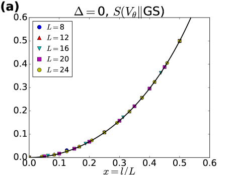
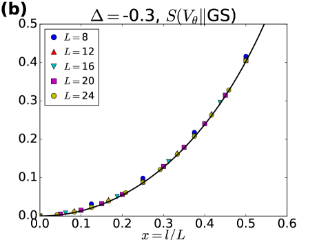
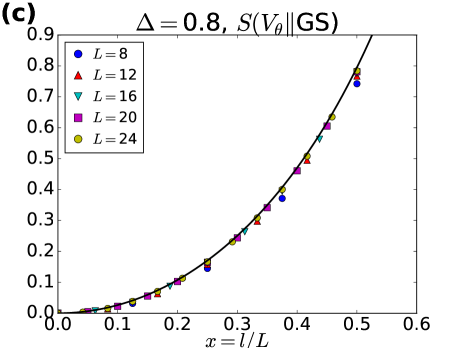
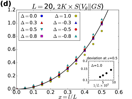
Figure 1: (a)(b)(c) Numerical results of the relative entropy between $V_{\theta}$ and the ground state of the XXZ chain for several values of $\Delta$ and $L$. Lines are the CFT prediction (20) with $\Delta_{V}=1/(4K)$. (d) Plot of $2K\times S(\rho_{V_{\theta}}\|\rho_{\mathrm{GS}})$, which is expected to be independent of $\Delta$ from the CFT prediction, $1-\pi x\cot(\pi x)$ (line). The inset shows the deviations of the numerical data of $\Delta=1.0$ from the CFT prediction at $x=0.5$.

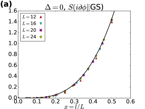
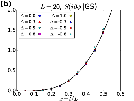
Figure 2: Numerical results of the relative entropy between $i\partial\phi$ and the ground state of the XXZ chain for (a) several $L$ with $\Delta=0$ and (b) several $\Delta$ with $L=20$. Lines are the CFT prediction (24).

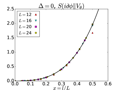
Figure 3: Numerical results of the relative entropy between the $i\partial\phi$ and $V_{\theta}$ of the XXZ chain at $\Delta=0$. Line is the CFT prediction (28).

In Fig. 1, we show the numerical results of $S(\rho_{V_{\theta}}\|\rho_{\mathrm{GS}})$ for several values of $\Delta$ and $L$. The numerical data perfectly agree with the CFT predictions ((20) with $\Delta_{V}=1/(4K)$ and note that $K$ depends on $\Delta$). We observe that the finite size effect (deviation from the CFT predictions) is stronger for larger $|\Delta|$ (see Fig. 1(d)). We think this is a consequence of the irrelevant term coming from $\Delta\sum_{i}S_{i}^{z}S_{i+1}^{z}$ in the derivation of the continuum field theory (13) from the lattice model (45) [39].

Next, in Fig. 2, we present the numerical results of $S(\rho_{i\partial\phi}\|\rho_{\mathrm{GS}})$. Agreement between the numerical data and the CFT prediction is again quite well.

Finally, we show the numerical data of $S(\rho_{i\partial\phi}\|\rho_{V_{\theta}})$ in Fig. 3. We confirm the CFT prediction (28), $S(\rho_{i\partial\phi}\|\rho_{V_{\theta}})=S(\rho_{i\partial\phi}\|\rho_{\mathrm{GS}})+S(\rho_{V_{\theta}}\|\rho_{\mathrm{GS}})$.

5.1.2 Sandwiched Rényi relative entropy.

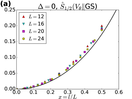
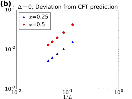
Figure 4: (a) Numerical results of the sandwiched Rényi relative entropy of the order of $\alpha=1/2$ between $V_{\theta}$ and the ground state of the XXZ chain ($\hat{S}_{1/2}(\rho_{V_{\theta}}\|\rho_{\mathrm{GS}})$). Line is the CFT prediction (46). (b) The deviation of the numerical data from the CFT prediction at $x=0.25$ and $x=0.5$.

As mentioned in the introduction, the meaning of the Rényi relative entropy (2), if any, has not been revealed yet from the viewpoint of quantum information theory. Here we numerically calculate the sandwiched Rényi relative entropy (11) which was shown to have desirable properties in quantum information theory [32] by taking advantage of exact diagonalization.

In [29] Lashkari derived a formula of the sandwiched Rényi relative entropy of the order of $\alpha=1/2$ between the vertex operator and the ground state in $c=1$ CFT and the result leads to

$$\hat{S}_{1/2}(\rho_{V_{\theta}}\|\rho_{\mathrm{GS}})=-2\Delta_{\theta}\log\left(\cos(\pi x/2)\right).$$ (46)

We numerically calculate $\hat{S}_{1/2}(\rho_{V_{\theta}}\|\rho_{\mathrm{GS}})$ in the XXZ chain and compare it with the prediction by CFT (Fig. 4). We observe that the numerical data match the CFT prediction although the finite size effect is larger than that of the relative entropies calculated in the above.

5.2 Critical transverse field Ising chain: the $c=1/2$ Ising CFT

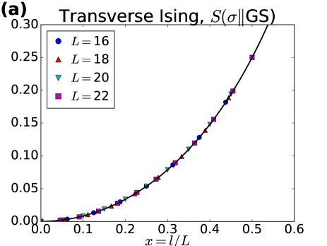
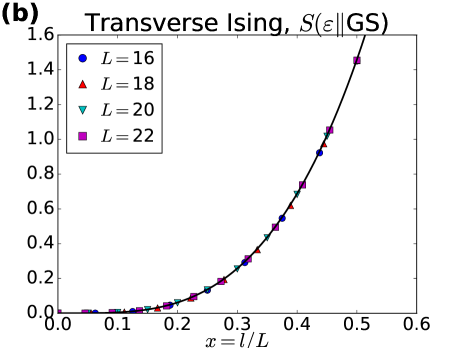
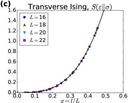
Figure 5: Numerical results of the relative entropy among the primary states $\sigma,\varepsilon$, and the ground state of the critical transverse field Ising chain: (a) $S(\rho_{\sigma}\|\rho_{\mathrm{GS}})$, (b) $S(\rho_{\varepsilon}\|\rho_{\mathrm{GS}})$, and (c) $S(\rho_{\varepsilon}\|\rho_{\sigma})$. Lines are the CFT predictions (37), (40), (44) (note that $S(\rho_{\sigma}\|\rho_{\mathrm{GS}})=S(\rho_{\mathrm{GS}}\|\rho_{\sigma})$ holds again as in the case of $c=1$ CFT [28]).

The next example where we compare numerical results of a lattice model with CFT predictions is the critical transverse field Ising chain under periodic boundary condition,

$$H=\sum_{i=1}^{L}\left(S^{x}_{i}S^{x}_{i+1}+0.5S^{z}_{i}\right).$$ (47)

The low-energy physics of this model is described by the $c=1/2$ Ising CFT (29). We perform exact diagonalization of this model and calculate the relative entropies between the eigenstates corresponding the primary states $\sigma,\varepsilon$ in the same way as the XXZ chain. Specifically, when $L$ is even, the ground state is in the sector of the momentum $k=0$ while the primary state $\sigma$ ($\varepsilon$) is obtained as the ground state (the first excited state) of the sector of the momentum $k=\pi\>(0)$.

In Fig. 5, the numerical results for $S(\rho_{\sigma}\|\rho_{\mathrm{GS}}),S(\rho_{\varepsilon}\|\rho_{\mathrm{GS}})$, and $S(\rho_{\varepsilon}\|\rho_{\sigma})$ are presented. The agreement between the CFT predictions and the numerical data is remarkably well.

6 Discussions and outlook

In this work we investigated the relative entropies between several primary states in the critical spin chains and compared them with the predictions by corresponding CFTs. After reviewing the results of [28] for $c=1$ free boson CFT we analytically derived the formulae of the relative entropy in the $c=1/2$ Ising CFT. Then we numerically calculated the relative entropy between several eigenstates in two critical spin chains, the $S=1/2$ XXZ chain and the critical transverse field Ising chain, by exact diagonalization. We saw perfect agreements of the numerical results with the CFT predictions in both models. Our numerical results extend those of [28] to the relative entropy itself rather than the Rényi counterpart of it and to interacting lattice systems. Our results establish further confirmation on the correspondence of the low-energy physics and the structure of entanglement between critical lattice systems and appropriate CFTs.

As a future direction, it would be interesting to extend our results to models corresponding to more complicated (1+1)-dimensional CFTs such as the minimal CFTs of $c=7/10,4/5,\cdots$ or level-$k$ Wess-Zumino-Witten model. Another direction of interest is to investigate the relative entropy in higher dimensions where little is known in the literature [21].

References

References

- [1] C. Holzhey, F. Larsen, and F. Wilczek, “Geometric and renormalized entropy in conformal field theory,” Nucl. Phys. B424 (1994) 443–467, arXiv:hep-th/9403108 [hep-th].
- [2] P. Calabrese and J. L. Cardy, “Entanglement entropy and quantum field theory,” J. Stat. Mech. 0406 (2004) P06002, arXiv:hep-th/0405152 [hep-th].
- [3] P. Calabrese and J. Cardy, “Entanglement entropy and conformal field theory,” J. Phys. A42 (2009) 504005, arXiv:0905.4013 [cond-mat.stat-mech].
- [4] A. Kitaev and J. Preskill, “Topological entanglement entropy,” Phys. Rev. Lett. 96 (2006) 110404, arXiv:hep-th/0510092 [hep-th].
- [5] M. Levin and X.-G. Wen, “Detecting Topological Order in a Ground State Wave Function,” Physical Review Letters 96 no. 11, (Mar., 2006) 110405, cond-mat/0510613.
- [6] J. M. Maldacena, “The Large N limit of superconformal field theories and supergravity,” Int. J. Theor. Phys. 38 (1999) 1113–1133, arXiv:hep-th/9711200 [hep-th]. [Adv. Theor. Math. Phys.2,231(1998)].
- [7] S. Ryu and T. Takayanagi, “Holographic derivation of entanglement entropy from AdS/CFT,” Phys. Rev. Lett. 96 (2006) 181602, arXiv:hep-th/0603001 [hep-th].
- [8] S. Ryu and T. Takayanagi, “Aspects of Holographic Entanglement Entropy,” JHEP 08 (2006) 045, arXiv:hep-th/0605073 [hep-th].
- [9] J. Maldacena and L. Susskind, “Cool horizons for entangled black holes,” Fortsch. Phys. 61 (2013) 781–811, arXiv:1306.0533 [hep-th].
- [10] H. Araki, “Relative entropy of states of von neumann algebras,” Publications of the Research Institute for Mathematical Sciences 11 no. 3, (1976) 809–833.
- [11] A. Wehrl, “General properties of entropy,” Rev. Mod. Phys. 50 (Apr, 1978) 221–260. https://link.aps.org/doi/10.1103/RevModPhys.50.221.
- [12] H. Casini, M. Huerta, and J. A. Rosabal, “Remarks on entanglement entropy for gauge fields,” Phys. Rev. D89 no. 8, (2014) 085012, arXiv:1312.1183 [hep-th].
- [13] T. Faulkner, R. G. Leigh, O. Parrikar, and H. Wang, “Modular Hamiltonians for Deformed Half-Spaces and the Averaged Null Energy Condition,” JHEP 09 (2016) 038, arXiv:1605.08072 [hep-th].
- [14] H. Casini, I. S. Landea, and G. Torroba, “The g-theorem and quantum information theory,” JHEP 10 (2016) 140, arXiv:1607.00390 [hep-th].
- [15] H. Casini, E. Teste, and G. Torroba, “Relative entropy and the RG flow,” arXiv:1611.00016 [hep-th].
- [16] R. Bousso, H. Casini, Z. Fisher, and J. Maldacena, “Proof of a Quantum Bousso Bound,” Phys. Rev. D90 no. 4, (2014) 044002, arXiv:1404.5635 [hep-th].
- [17] H. Casini, E. Teste, and G. Torroba, “The a-theorem and the Markov property of the CFT vacuum,” arXiv:1704.01870 [hep-th].
- [18] V. Vedral, “The role of relative entropy in quantum information theory,” Rev. Mod. Phys. 74 (2002) 197–234.
- [19] N. Lashkari, “Modular Hamiltonian for Excited States in Conformal Field Theory,” Phys. Rev. Lett. 117 no. 4, (2016) 041601, arXiv:1508.03506 [hep-th].
- [20] G. Sárosi and T. Ugajin, “Relative entropy of excited states in two dimensional conformal field theories,” JHEP 07 (2016) 114, arXiv:1603.03057 [hep-th].
- [21] G. Sárosi and T. Ugajin, “Relative entropy of excited states in conformal field theories of arbitrary dimensions,” JHEP 02 (2017) 060, arXiv:1611.02959 [hep-th].
- [22] G. Sárosi and T. Ugajin, “Modular Hamiltonians of excited states, OPE blocks and emergent bulk fields,” arXiv:1705.01486 [hep-th].
- [23] T. Ugajin, “Mutual information of excited states and relative entropy of two disjoint subsystems in CFT,” arXiv:1611.03163 [hep-th].
- [24] J. Lin, M. Marcolli, H. Ooguri, and B. Stoica, “Locality of Gravitational Systems from Entanglement of Conformal Field Theories,” Phys. Rev. Lett. 114 (2015) 221601, arXiv:1412.1879 [hep-th].
- [25] D. L. Jafferis, A. Lewkowycz, J. Maldacena, and S. J. Suh, “Relative entropy equals bulk relative entropy,” JHEP 06 (2016) 004, arXiv:1512.06431 [hep-th].
- [26] N. Lashkari, J. Lin, H. Ooguri, B. Stoica, and M. Van Raamsdonk, “Gravitational Positive Energy Theorems from Information Inequalities,” arXiv:1605.01075 [hep-th].
- [27] P. Caputa and M. M. Rams, “Quantum dimensions from local operator excitations in the Ising model,” J. Phys. A50 no. 5, (2017) 055002, arXiv:1609.02428 [cond-mat.str-el].
- [28] P. Ruggiero and P. Calabrese, “Relative Entanglement Entropies in 1+1-dimensional conformal field theories,” JHEP 02 (2017) 039, arXiv:1612.00659 [hep-th].
- [29] N. Lashkari, “Relative Entropies in Conformal Field Theory,” Phys. Rev. Lett. 113 (2014) 051602, arXiv:1404.3216 [hep-th].
- [30] M. Müller-Lennert, F. Dupuis, O. Szehr, S. Fehr, and M. Tomamichel, “On quantum rényi entropies: A new generalization and some properties,” Journal of Mathematical Physics 54 no. 12, (2013) 122203.
- [31] M. M. Wilde, A. Winter, and D. Yang, “Strong converse for the classical capacity of entanglement-breaking and hadamard channels via a sandwiched rényi relative entropy,” Communications in Mathematical Physics 331 no. 2, (2014) 593–622.
- [32] R. L. Frank and E. H. Lieb, “Monotonicity of a relative Rényi entropy,” Journal of Mathematical Physics 54 no. 12, (Dec., 2013) 122201–122201, arXiv:1306.5358 [math-ph].
- [33] F. C. Alcaraz, M. I. Berganza, and G. Sierra, “Entanglement of low-energy excitations in Conformal Field Theory,” Phys. Rev. Lett. 106 (2011) 201601, arXiv:1101.2881 [cond-mat.stat-mech].
- [34] M. I. Berganza, F. C. Alcaraz, and G. Sierra, “Entanglement of excited states in critical spin chians,” J. Stat. Mech. 1201 (2012) P01016, arXiv:1109.5673 [cond-mat.stat-mech].
- [35] M. A. Nielsen and I. L. Chuang, Quantum computation and quantum information. Cambridge university press, 2010.
- [36] F. H. L. Essler, A. M. Läuchli, and P. Calabrese, “Shell-Filling Effect in the Entanglement Entropies of Spinful Fermions,” Physical Review Letters 110 no. 11, (Mar., 2013) 115701, arXiv:1211.2474 [cond-mat.str-el].
- [37] P. Calabrese, F. H. L. Essler, and A. M. Läuchli, “Entanglement entropies of the quarter filled Hubbard model,” Journal of Statistical Mechanics: Theory and Experiment 9 (Sept., 2014) 09025, arXiv:1406.7477 [cond-mat.str-el].
- [38] P. Di Francesco, P. Mathieu, and D. Senechal, Conformal Field Theory. Graduate Texts in Contemporary Physics. Springer-Verlag, New York, 1997. http://www-spires.fnal.gov/spires/find/books/www?cl=QC174.52.C66D5::1997.
- [39] T. Giamarchi, Quantum physics in one dimension. No. 121 in The international series of monographs on physics. Clarendon Press, 2004. http://ci.nii.ac.jp/ncid/BA65805043.
- [40] J. L. Cardy, “Logarithmic corrections to finite-size scaling in strips,” Journal of Physics A: Mathematical and General 19 no. 17, (1986) L1093. http://stacks.iop.org/0305-4470/19/i=17/a=008.