FlavBit: A GAMBIT module for computing flavour observables and likelihoods

Abstract

Flavour physics observables are excellent probes of new physics up to very high energy scales. Here we present FlavBit, the dedicated flavour physics module of the global-fitting package GAMBIT. FlavBit includes custom implementations of various likelihood routines for a wide range of flavour observables, including detailed uncertainties and correlations associated with LHCb measurements of rare, leptonic and semileptonic decays of $B$ and $D$ mesons, kaons and pions. It provides a generalised interface to external theory codes such as SuperIso, allowing users to calculate flavour observables in and beyond the Standard Model, and then test them in detail against all relevant experimental data. We describe FlavBit and its constituent physics in some detail, then give examples from supersymmetry and effective field theory illustrating how it can be used both as a standalone library for flavour physics, and within GAMBIT.

1 Introduction

Precise measurement of flavour observables is a powerful indirect probe of physics beyond the Standard Model (SM), as new heavy particles predicted by extensions of the SM can contribute to the amplitudes of observables as virtual particles. Flavour observables are therefore sensitive to much higher energy scales than direct searches for new particles. Moreover, rare decays, such as Flavour Changing Neutral Currents (FCNCs), are loop suppressed in the SM. As a consequence, the SM decay rates are small, and could be comparable in magnitude to contributions from new heavy states, allowing stringent constraints to be placed on the parameters of theories for new physics. It is therefore crucial to consider constraints from flavour physics when studying scenarios beyond the SM. The correlations between the different flavour observables, and the interplay between flavour measurements and direct searches at collider experiments, are key tools in the search for new physics, and its eventual understanding.

Public packages exist for carrying out SM and BSM flavour fits in terms of Wilson coefficients Serra:2016ivr ; flavio ; hepfit , but so far no general package exists for both computing Wilson coefficients and carrying out a global fit. In this article we present FlavBit, a flavour physics library designed in the context of the Global And Modular BSM Inference Tool (GAMBIT) framework gambit , but also usable in standalone form. FlavBit allows users to predict flavour physics observables in various models, using external programs such as SuperIso Mahmoudi:2007vz ; Mahmoudi:2008tp ; Mahmoudi:2009zz , and then calculate combined likelihoods for arbitrary combinations of the observables. FlavBit takes into account all theoretical and experimental correlations between the different observables. The resulting likelihoods can be incorporated into the GAMBIT global likelihood to scan the parameter spaces of various models for new physics gambit ; ScannerBit ; SSDM ; CMSSM ; MSSM , taking into account complementary constraints from direct production ColliderBit , dark matter searches DarkBit , and SM and related precision measurements SDPBit .

Recently, some measurements of flavour observables, mainly from LHCb Aaij:2015esa ; Aaij:2015yra ; Aaij:2014ora ; Aaij:2013qta and $B$ factories Lees:2012xj ; Lees:2013uzd ; Huschle:2015rga ; Abdesselam:2016cgx ; Abdesselam:2016llu , have shown tension with their predicted values in the SM. It is still unclear if these might be accommodated in the SM by larger-than-expected QCD effects, statistical fluctuations or some combination thereof. Nonetheless, these tensions certainly provide motivation for continued interest and effort in careful combination and cross-correlation of flavour observables with each other, and with searches for new physics in other sectors. We include these measurements in FlavBit.

This paper is organised as follows. In Sec. 2 we provide the general theoretical background of the scheme by which we compute flavour observables, before providing a brief synopsis in Sec. 3 of the broader global-fitting framework within which FlavBit sits. In Sec. 4 we discuss the predictions and measurements of individual observables included in FlavBit 1.0.0, and highlight aspects of new physics models to which the different measurements are sensitive. Sec. 5 gives details of the likelihood calculations that FlavBit performs. Sec. 6 gives some usage examples, both in standalone mode and with GAMBIT proper. Sec. 7 summarises our conclusions, and Appendix A gives a glossary of relevant GAMBIT terminology helpful for reading this paper.

The FlavBit source code is freely available from gambit.hepforge.org under the terms of the standard 3-clause BSD license.

2 Theoretical framework

Our theoretical framework for studying rare decay observables is based on the effective Hamiltonian approach, which provides a simple formulation that can be easily extended to incorporate contributions from new physics. In this formulation, the low- and high-energy effects are separated using the Operator Product Expansion method. Cross-sections for transitions from initial states $i$ to final states $f$ are proportional to squared matrix elements $|\langle f|{\cal H}_{\rm eff}|i\rangle|^{2}$, where the effective Hamiltonian ${\cal H}_{\rm eff}$ for $b\rightarrow s$ transitions is given by

$$\mathcal{H}_{\rm eff}=-\frac{4G_{F}}{\sqrt{2}}V_{tb}V_{ts}^{*}\sum_{i=1}^{10}\Bigl{(}C_{i}(\mu)\mathcal{O}_{i}(\mu)+C^{\prime}_{i}(\mu)\mathcal{O}^{\prime}_{i}(\mu)\Bigr{)}\;.$$ (1)

Here $G_{\text{F}}$ is the Fermi constant, $\mu$ is the energy scale at which calculations are to be performed, and $V_{tb}$ and $V_{ts}$ are the usual CKM matrix elements. The $C_{i}$ are Wilson coefficients, which incorporate the influence of small-scale physics due to heavy states that have been integrated out in the effective theory; their values can be calculated using perturbative methods. The $\mathcal{O}_{i}$ are local operators representing long-distance interactions. The most relevant operators for the FCNC rare $B$ decays are

$$\mathcal{O}_{1} =(\bar{s}\gamma_{\mu}T^{a}P_{L}c)(\bar{c}\gamma^{\mu}T^{a}P_{L}b)\;,$$

$$\mathcal{O}_{2} =(\bar{s}\gamma_{\mu}P_{L}c)(\bar{c}\gamma^{\mu}P_{L}b)\;,$$

$$\mathcal{O}_{3} =(\bar{s}\gamma_{\mu}P_{L}b)\sum_{q}(\bar{q}\gamma^{\mu}q)\;,$$

$$\mathcal{O}_{4} =(\bar{s}\gamma_{\mu}T^{a}P_{L}b)\sum_{q}(\bar{q}\gamma^{\mu}T^{a}q)\;,$$

$$\mathcal{O}_{5} =(\bar{s}\gamma_{\mu_{1}}\gamma_{\mu_{2}}\gamma_{\mu_{3}}P_{L}b)\sum_{q}(\bar{q}\gamma^{\mu_{1}}\gamma^{\mu_{2}}\gamma^{\mu_{3}}q)\;,$$

$$\mathcal{O}_{6} =(\bar{s}\gamma_{\mu_{1}}\gamma_{\mu_{2}}\gamma_{\mu_{3}}T^{a}P_{L}b)\sum_{q}(\bar{q}\gamma^{\mu_{1}}\gamma^{\mu_{2}}\gamma^{\mu_{3}}T^{a}q)\;,$$

$$\mathcal{O}_{7} =\frac{e}{(4\pi)^{2}}m_{b}(\overline{s}\sigma^{\mu\nu}P_{R}b)F_{\mu\nu}\;,$$

$$\mathcal{O}_{8} =\frac{g}{(4\pi)^{2}}m_{b}(\bar{s}\sigma^{\mu\nu}T^{a}P_{R}b)G_{\mu\nu}^{a}\;,$$

$$\mathcal{O}_{9} =\frac{e^{2}}{(4\pi)^{2}}(\overline{s}\gamma^{\mu}P_{L}b)(\bar{\ell}\gamma_{\mu}\ell)\;,$$

$$\mathcal{O}_{10} =\frac{e^{2}}{(4\pi)^{2}}(\overline{s}\gamma^{\mu}P_{L}b)(\bar{\ell}\gamma_{\mu}\gamma_{5}\ell)\;,$$ (2)

where the sums run over $q=u,d,s,c,b$, $m_{b}$ denotes the $b$ quark mass, $T^{a}$ are the SU(3)_c generators, $F_{\mu\nu}$ and $G_{\mu\nu}^{a}$ are the photon and gluon stress-energy tensors respectively, and $g$ is the strong coupling. A similar set of operators can also be defined for $b\rightarrow d$ transitions.

This formalism can be easily extended to incorporate effects of new physics, through additional contributions to the Wilson coefficients or the introduction of additional long-distance operators. For instance, the primed versions of these operators are chirality-flipped compared to the non-primed ones, and are highly suppressed in the SM. The scalar ($\mathcal{Q}_{1}$) and pseudoscalar ($\mathcal{Q}_{2}$) operators

$$\mathcal{Q}_{1} =\frac{e^{2}}{(4\pi)^{2}}(\bar{s}P_{R}b)(\bar{\ell}\,\ell)\;,$$ (3)

$$\mathcal{Q}_{2} =\frac{e^{2}}{(4\pi)^{2}}(\bar{s}P_{R}b)(\bar{\ell}\gamma_{5}\ell)\;,$$ (4)

are absent in the SM, but receive large contributions in many models with an extended Higgs sector.

The Wilson coefficients are calculated by requiring matching between the high-scale theory and the low-energy effective theory at the scale $\mu_{W}$, which is of the order of the $W$ mass. Using the renormalisation group equations of the effective theory, they are then evolved to the scale $\mu_{b}$ (of the order of the $b$ quark mass), which is the relevant scale for $B$ physics calculations.

In order to compute the matrix element $\langle f|{\cal H}_{\rm eff}|i\rangle$, which describes the transition from the initial state $|i\rangle$ to the final state $|f\rangle$, in addition to the relevant Wilson coefficients $C_{i}$, we need to evaluate the hadronic matrix elements $\langle f|{\cal O}_{i}|i\rangle$, which are usually the main source of uncertainties. These elements lead to decay constants and form factors that must be computed with techniques from non-perturbative QCD.

3 Computational framework

The GAMBIT framework defines two sorts of functions that can be used to calculate physical observables or other quantities required for computing them:

module functions:

functions written in C++ and contained within a GAMBIT module.

backend functions:

external library functions provided by a backend, such as SuperIso or FeynHiggs.

For ease of reference, here we highlight and link specific GAMBIT terms to their entries in the glossary, found in Appendix A.

When writing GAMBIT module functions, the author assigns each a capability, which describes what the function can calculate. This may be an observable, e.g. a particular branching fraction for a given rare $B$ decay, or a likelihood, e.g. the combined likelihood defined using a set of rare decays. Module functions can be declared to have dependencies on the results of other module functions, which they indicate by specifying the capability of the module function that must be used to fill the dependency. Dependencies may be filled by any function within GAMBIT that has the requisite capability, whether or not it is part of the same GAMBIT module as the dependent function. Module functions may also have backend requirements, which are satisfied by functions from backend libraries. For example, in FlavBit 1.0.0, SuperIso supplies many of the backend requirements of the module functions that calculate observables.

FlavBit notifies GAMBIT of its available module functions and their capabilities, dependencies and backend requirements. The user tells GAMBIT that they want to compute a given set of observables and likelihoods in a given scan, and the GAMBIT Core identifies the necessary module functions and runs its dependency resolution routines. These hook the module functions up to each other and run them in an order that ensures that all dependencies are computed before the functions that depend on them. Full details of this process can be found in the main GAMBIT paper gambit .

In standalone mode, users can just call the module functions of FlavBit directly, providing any required dependencies and backend requirements manually.

4 Observables

In this section we discuss the observables included in FlavBit and their relevance for searches for new physics.

The most important observables are the rare decays $B\rightarrow X_{s}\gamma$, $B^{0}_{s}\rightarrow\mu^{+}\mu^{-}$ and $B^{0}\rightarrow K^{*0}\mu^{+}\mu^{-}$, as well as tree level decays such as $B^{\pm}\rightarrow\tau\nu_{\tau}$ and $B\rightarrow D^{(*)}\ell\nu_{\ell}$.

Here we discuss the calculation of the different observables in four groups: tree-level leptonic and semi-leptonic decays (Sec. 4.2), electroweak penguin transitions (Sec. 4.3), rare purely leptonic decays (Sec. 4.4), and other flavour observables (Sec. 4.5). In these sections we outline the calculations required to predict each observable from theory; further details can be found in Ref. Mahmoudi:2008tp . While for simplicity we present only the leading order expressions in this paper, in FlavBit itself we use the full calculations at the highest available accuracy.

The tree-level category includes $B$ and $D$ decays to leptons with an accompanying hadron and/or a neutrino in the final state. Observables in this category are the branching fractions for processes such as $B^{\pm}\rightarrow\tau\nu_{\tau}$, $B\rightarrow D^{(*)}\tau\nu_{\tau}$ and $B\rightarrow D^{(*)}\ell\nu_{\ell}$. The electroweak penguin category includes the rare decays $B\rightarrow M\ell^{+}\ell^{-}$ (with $M$ another meson lighter than the $B$), in particular the angular observables of the decay $B^{0}\rightarrow K^{*0}\mu^{+}\mu^{-}$. The rare fully-leptonic category includes $B$ decays with only leptons in the final state, such as $B^{0}_{(s)}\rightarrow\mu^{+}\mu^{-}$. The fourth and final category includes $b\rightarrow s$ transitions in the radiative decays $B\rightarrow X_{s}\gamma$, the mass difference between the heavy $B_{H}$ and light $B_{L}$ eigenstates of the $B^{0}_{s}$ system ($\Delta M_{s}$), and decays of kaons and pions, in particular the leptonic decay ratio ${\cal B}(K^{\pm}\rightarrow\mu\nu_{\mu})/{\cal B}(\pi^{\pm}\rightarrow\mu\nu_{\mu})$. Note that FlavBit does not incorporate the anomalous magnetic moment of the muon, as this is dealt with in PrecisionBit SDPBit .

4.1 Interfaces to external codes

Theoretical predictions of observables in FlavBit are predominantly obtained through interfaces to external codes. Some predictions of flavour observables are available from FeynHiggs Heinemeyer:1998yj , for the SM and minimal supersymmetric SM (MSSM). In FlavBit 1.0.0, most observable calculations refer to SuperIso 3.6 Mahmoudi:2007vz ; Mahmoudi:2008tp ; Mahmoudi:2009zz .

The interface to SuperIso operates via the function SI_fill (see Table 1), which provides the SuperIso_modelinfo. This function fills a SuperIso parameters structure, which is passed back to various other SuperIso functions to compute observables. Observables that are calculated directly from the input model parameters (Table 1) are distinguished from those that involve the calculation of intermediate Wilson coefficients (Tables 2 and 3). In FlavBit 1.0.0, observables are implemented for MSSM models (‘MSSM63atQ’ and descendants; see gambit ), and for a flavour EFT model (‘WC’) where the Wilson coefficients are specified directly as model parameters, and scanned over.

The design of FlavBit and its interface to SuperIso make extending FlavBit to other models quite straightforward, either by computing Wilson coefficients ‘upstream’ from fundamental parameters, or by constructing the SuperIso_modelinfo to fit the model under investigation. SI_fill deals with the majority of the model-dependence in each calculation, importing different masses and couplings from SpecBit depending on the model being scanned, and using them to set various flags and member variables of the SuperIso_modelinfo.

SI_fill has a single option configurable from the master YAML file of a given scan: a boolean flag take_b_pole_mass_from_spectrum. This option allows the user to choose between SuperIso’s internal calculation of the $b$ quark pole mass (based on the $\overline{MS}$ mass imported from GAMBIT), or GAMBIT’s own $b$ pole mass calculation provided by SpecBit SDPBit . Depending on the spectrum generator chosen in SpecBit, the standard 2-loop conversion from $\overline{MS}$ to pole mass included in SuperIso may be a more accurate choice for precision $B$ physics than other calculations, even if the other calculation includes higher-order corrections. This is because the $b$ pole is sufficiently close to the QCD scale that problems with the perturbative expansion required to compute it start to show already at 3 loops Olive:2016xmw , such that the formal error on the $b$ pole mass associated with truncating the asymptotic series may already be larger when truncating at 3 rather than 2 loops. This means that although 3-loop QCD RGEs remain preferable, 2-loop self energies give a more precise value for the $b$ pole, and should be preferred for $B$ physics calculations. In FlavBit 1.0.0, take_b_pole_mass_from_spectrum therefore defaults to false.

Capability	Function (Return Type): Brief Description	Dependencies (Model)	Backend requirements
SuperIso_modelinfo	SI_fill (parameters): Fills the SuperIso structure. Key routine of the SuperIso interface.	MSSM_spectrum (MSSM63atQ)	Init_param
		SM_spectrum (WC)	slha_adjust
		W_plus_decay_rates	mb_1S
		Z_decay_rates
Dstaunu	SI_Dstaunu (double): Computes the branching fraction of $D^{\pm}_{s}\rightarrow\tau\nu_{\tau}$.	SuperIso_modelinfo	Dstaunu
Dsmunu	SI_Dsmunu (double): Computes the branching fraction of $D^{\pm}_{s}\rightarrow\mu\nu_{\mu}$.	SuperIso_modelinfo	Dsmunu
Dmunu	SI_Dmunu (double): Computes the branching fraction of $D^{\pm}\rightarrow\mu\nu_{\mu}$.	SuperIso_modelinfo	Dmunu
Btaunu	SI_Btaunu (double): Computes the branching fraction of $B^{\pm}\rightarrow\tau\nu_{\tau}$.	SuperIso_modelinfo	Btaunu
BDtaunu	SI_BDtaunu (double): Computes the branching fraction of $B\rightarrow D\tau\nu_{\tau}$.	SuperIso_modelinfo	BRBDlnu
BDmunu	SI_BDmunu (double): Computes the branching fraction of $B\rightarrow D\mu\nu_{\mu}$.	SuperIso_modelinfo	BRBDlnu
BDstartaunu	SI_BDstartaunu (double): Computes the branching fraction of $B\rightarrow D^{*}\tau\nu_{\tau}$.	SuperIso_modelinfo	BRBDstarlnu
BDstarmunu	SI_BDstarmunu (double): Computes the branching fraction of $B\rightarrow D^{*}\mu\nu_{\mu}$.	SuperIso_modelinfo	BRBDstarlnu
RD	SI_RD (double): Computes the ratio $\mathcal{B}(B\rightarrow D\tau\nu_{\tau})/\mathcal{B}(B\rightarrow Dl\nu_{l})$, where $\ell=\mu$ or $e$ and the result is the same for each.	SuperIso_modelinfo	BDtaunu_BDenu
RDstar	SI_RDstar (double): Computes the ratio $\mathcal{B}(B\rightarrow D^{*}\tau\nu_{\tau})/\mathcal{B}(B\rightarrow D^{*}l\nu_{l})$, where $\ell=\mu$ or $e$ and the result is the same for each.	SuperIso_modelinfo	BDstartaunu_
			BDstarenu
Rmu	SI_Rmu (double): Computes the ratio $\mathcal{B}(K^{\pm}\rightarrow\mu\nu_{\mu})/\mathcal{B}(\pi^{\pm}\rightarrow\mu\nu_{\mu})$.	SuperIso_modelinfo	Kmunu_pimunu
Rmu23	SI_Rmu23 (double): Computes the observable $R_{\mu 23}$ (Eq. 32).	SuperIso_modelinfo	Rmu23
FH_FlavourObs	FH_FlavourObs (fh_FlavourObs): Computes the FeynHiggs flavour observables.		FHFlavour
deltaMs	FH_DeltaMs (double): Extracts the FeynHiggs MSSM prediction for the $B_{s}$–$\bar{B}_{s}$ mass difference $\Delta M_{s}$ (in ps-1).	FH_FlavourObs

Table 1: Observable capabilities of FlavBit that do not involve Wilson coefficients. Details of the fh_FlavourObs structure can be found in Table 8.

4.2 Tree-level leptonic and semi-leptonic decays

Decays of $B$ mesons with leptons and neutrinos in the final state proceed via tree-level charged currents. They have been intensively studied at $B$ factories (Babar, Belle and CLEO) for the determination of the elements $V_{cb}$ and $V_{ub}$ of the CKM matrix.

The rate of the semi-leptonic decay $B\rightarrow M\ell\nu_{\ell}$ in the SM is

$$\frac{d\Gamma}{dq^{2}}=\frac{G_{F}^{2}|V_{qb}^{2}|}{192\pi^{3}m_{B}^{3}}{\cal K}(m^{2}_{B},m^{2}_{M},q^{2}){\cal F}^{(2)}(q^{2})\;,$$ (5)

where $q^{\mu}=p_{B}^{\mu}-p^{\mu}_{M}$ is the momentum transfer, $V_{qb}$ is the CKM element corresponding to the flavour of $M$, ${\cal K}$ is a phase-space factor and ${\cal F}^{(2)}(q^{2})$ is a combination of form factors Sakaki:2013bfa .

These decays are sensitive to charged-current contributions from new particles. For example, the charged Higgs in the two Higgs doublet model (2HDM) (see e.g. Refs. Crivellin:2015hha ; Freytsis:2015qca ; Buras:2013ooa ; Eberhardt:2013uba ), right-handed currents via the contribution of the charged mediator $W_{R}$ Das:2016vkr ; Buras:2013ooa , new left-handed heavy bosons $W^{\prime}$ Greljo:2015mma ; Boucenna:2016qad and leptoquarks (see e.g. Refs. Becirevic:2016oho ; Dorsner:2016wpm ) can also modify the value of this observable.

The decays $B^{\pm}\rightarrow\ell\nu_{\ell}$ also proceed via tree-level charged currents. The branching fraction is

$${\cal B}(B^{+}\rightarrow\ell^{+}\nu_{\ell})=\frac{G_{F}^{2}m_{B}m^{2}_{\ell}}{8\pi}\left(1-\frac{m_{\ell}^{2}}{m_{B}^{2}}\right)^{2}f_{B}^{2}|V_{ub}|^{2}\tau_{B},$$ (6)

where $f_{B}$ is the meson decay constant and $\tau_{B}$ is the lifetime of the $B^{+}$. This decay is sensitive to the CKM element $V_{ub}$. The charged Higgs sector of the 2HDM can again provide substantial contributions, as can new charged gauge bosons like the $W^{\prime}$ and $W_{R}$ of the left-right symmetric model Bona:2009cj . Compared to the case where $\ell=\tau$, the decays with $\ell=e$ and $\ell=\mu$ have much smaller branching fractions, as they are helicity-suppressed. For this reason, at present only upper limits are available for the decays to light leptons. Although we provide routines to predict the values of all three in FlavBit, we only incorporate the tauonic version into the resulting likelihood.

Similarly, the decays $D^{\pm}_{(s)}\rightarrow\ell\nu_{\ell}$ are mediated by the $W$ boson in the SM. The branching fractions can be obtained from Eq. 6 after the replacement $B\rightarrow D_{(s)}$ and swapping in the relevant CKM element. These decays have been traditionally used to measure the $D_{(s)}$ meson decay constant. However, the charged Higgs boson in the 2HDM would also mediate these decays, so they can provide complementary constraints to the analogous $B$ meson decay Akeroyd:2009tn .

As shown in Table 1, FlavBit provides functions capable of computing branching fractions for $D^{\pm}_{s}\rightarrow\tau\nu_{\tau}$ (Dstaunu), $D^{\pm}_{s}\rightarrow\mu\nu_{\mu}$ (Dsmunu), $D^{\pm}\rightarrow\mu\nu_{\mu}$ (Dmunu), $B^{\pm}\rightarrow\tau\nu_{\tau}$ (Btaunu), $B\rightarrow D\tau\nu_{\tau}$ (BDtaunu), $B\rightarrow D\mu\nu_{\mu}$ (BDmunu), $B\rightarrow D^{*}\tau\nu_{\tau}$ (BDstartaunu) and $B\rightarrow D^{*}\mu\nu_{\mu}$ (BDstarmunu). It can also compute $R_{D^{(*)}}\equiv\mathcal{B}(B\rightarrow D^{(*)}\tau\nu_{\tau})/\mathcal{B}(B\rightarrow D^{(*)}l\nu_{l})$, designated by capabilities RD and RDstar. Here $\ell$ in $R_{D^{(*)}}$ refers to either $\mu$ or $e$, not their sum (the branching fractions $B\rightarrow D^{(*)}l\nu_{l}$ are identical for $e$ and $\mu$, as both are effectively massless in the $B$ system).

Capability	Function (Return Type): Brief Description	Dependencies	Backend requirements
bsgamma	SI_bsgamma (double): Computes the inclusive branching fraction of $B\rightarrow X_{s}\gamma$ for $E_{\gamma}>1.6$ GeV.	SuperIso_modelinfo	bsgamma_CONV
	FH_bsgamma (double): Extracts the total inclusive branching fraction of $B\rightarrow X_{s}\gamma$ in the MSSM from FeynHiggs.	FH_FlavourObs
delta0	SI_delta0 (double): Computes the isospin asymmetry of $B\rightarrow K^{*}\gamma$.	SuperIso_modelinfo	delta0_CONV
Bsmumu_untag	SI_Bsmumu_untag (double): Computes the $CP$-averaged branching fraction of $B^{0}_{s}\rightarrow\mu^{+}\mu^{-}$.	SuperIso_modelinfo	Bsll_untag_CONV
	FH_Bsmumu (double): Extracts the $CP$-averaged branching fraction of $B^{0}_{s}\rightarrow\mu^{+}\mu^{-}$ in the MSSM from FeynHiggs.	FH_FlavourObs
Bsee_untag	SI_Bsee_untag (double): Computes the $CP$-averaged branching fraction of $B^{0}_{s}\rightarrow e^{+}e^{-}$.	SuperIso_modelinfo	Bsll_untag_CONV
Bmumu	SI_Bmumu (double): Computes the branching fraction of $B^{0}\rightarrow\mu^{+}\mu^{-}$.	SuperIso_modelinfo	Bll_CONV
BRBXsmumu_lowq2	SI_BRBXsmumu_lowq2 (double): Computes the inclusive low-$q^{2}$ branching fraction of $B\rightarrow X_{s}\mu^{+}\mu^{-}$.	SuperIso_modelinfo	BRBXsmumu_lowq2_CONV
BRBXsmumu_highq2	SI_BRBXsmumu_highq2 (double): Computes the inclusive high-$q^{2}$ branching fraction of $B\rightarrow X_{s}\mu^{+}\mu^{-}$.	SuperIso_modelinfo	BRBXsmumu_high2_CONV
A_BXsmumu_lowq2	SI_A_BXsmumu_lowq2 (double): Computes the low-$q^{2}$ forward-backward asymmetry of $B\rightarrow X_{s}\mu^{+}\mu^{-}$.	SuperIso_modelinfo	A_BXsmumu_lowq2_CONV
A_BXsmumu_highq2	SI_A_BXsmumu_highq2 (double): Computes the high-$q^{2}$ forward-backward asymmetry of $B\rightarrow X_{s}\mu^{+}\mu^{-}$.	SuperIso_modelinfo	A_BXsmumu_highq2_CONV
A_BXsmumu_zero	SI_A_BXsmumu_zero (double): Computes the zero crossing $q^{2}$ value of the forward-backward asymmetry of $B\rightarrow X_{s}\mu^{+}\mu^{-}$.	SuperIso_modelinfo	A_BXsmumu_zero_CONV
BRBXstautau_highq2	SI_BRBXstautau_highq2 (double): Computes the inclusive high-$q^{2}$ branching fraction of $B\rightarrow X_{s}\tau^{+}\tau^{-}$.	SuperIso_modelinfo	BRBXstautau_highq2_CONV
A_BXstautau_highq2	SI_A_BXstautau_highq2 (double): Computes the high-$q^{2}$ forward-backward asymmetry of $B\rightarrow X_{s}\tau^{+}\tau^{-}$.	SuperIso_modelinfo	A_BXstautau_highq2_CONV

Table 2: Observable capabilities of FlavBit that involve Wilson coefficients in their calculation (from SuperIso unless otherwise specified).

Capability	Function (Return Type): Brief Description	Dependencies	Backend requirements
BKstarmumu_l_m	SI_BKstarmumu_l_m (Flav_KstarMuMu_obs): Computes all observables associated with $B^{0}\rightarrow K^{*0}\mu^{+}\mu^{-}$ in a $q^{2}$ bin specified by l and m. See caption for details.	SuperIso_modelinfo	SI_BKstarmumu_CONV
AI_BKstarmumu	SI_AI_BKstarmumu (double): Computes the low-$q^{2}$ isospin asymmetry of $B\rightarrow K^{*}\mu^{+}\mu^{-}$ (in GeV2).	SuperIso_modelinfo	AI_BKstarmumu_CONV
AI_BKstarmumu_zero	SI_AI_BKstarmumu_zero (double): Computes the zero-crossing $q^{2}$ value of the isospin asymmetry of $B\rightarrow K^{*}\mu^{+}\mu^{-}$.	SuperIso_modelinfo	AI_BKstarmumu_
			zero_CONV

Table 3: Observable capabilities of FlavBit related to the decay $B^{0}\rightarrow K^{*0}\mu^{+}\mu^{-}$. The indices l and m refer to the edges of the energy bin used in the particular function. The functions and capabilities are named such that l,m = 11,25 indicates an energy range of $1.1$–$2.5$ GeV², and so on. Possible pairs of l and m are (11,25), (25,40), (40,60), (60,80), (15,17) and (17,19); the last two refer to momentum transfer ranges of $15$–$17$–$19$ GeV².

Name (type)	Description
BR (double)	branching fraction
AFB (double)	forward-backward asymmetry
FL (double)	longitudinal fraction
S3 (double)	$S_{3}$
S4 (double)	$S_{4}$
S5 (double)	$S_{5}$
S7 (double)	$S_{7}$
S8 (double)	$S_{8}$
S9 (double)	$S_{9}$
q2_min (double)	$q^{2}$ bin lower edge
q2_max (double)	$q^{2}$ bin upper edge

Table 4: Observables contained in the Flav_KstarMuMu_obs structure.

4.3 Electroweak penguin transitions

Rare semi-leptonic decays of $B$ mesons proceed via flavour-changing neutral currents (FCNCs) in electroweak penguin diagrams, and set stringent constraints on possible contributions from new physics. FlavBit includes predictions of various FCNC $b\rightarrow s$ transitions. These decays are all proportional to the elements $V_{tb}$ and $V_{ts}$ of the CKM matrix.

Rare decays of the type $B\rightarrow M\ell^{+}\ell^{-}$, with one meson $M$ in the final state, are sensitive to the Wilson coefficients $C_{9,10}^{(\prime)}$. In addition, when $M$ is a vector, such as the $K^{*}(892)$, these decays are also sensitive to the Wilson coefficients $C_{7}^{(\prime)}$.

The four-quark operators ($\mathcal{O}_{1\cdots 6}$) in the effective Hamiltonian also contribute to the penguin diagrams, resulting in expressions with the same structure as $\mathcal{O}_{7}$ and $\mathcal{O}_{9}$. They can therefore be reabsorbed and used to define effective Wilson coefficients $C_{7}^{\rm eff}$ and $C_{9}^{\rm eff}$ Beneke:2001at ,

$$C_{7}^{\rm eff} = C_{7}-\frac{1}{3}C_{3}-\frac{4}{9}C_{4}-\frac{20}{3}C_{5}-\frac{80}{9}C_{6}\;,$$ (7)

$$C_{9}^{\rm eff} = C_{9}+Y(q^{2})\;,$$ (8)

where $Y$ contains the short distance contributions from the four-quark operators Greub:1994pi ; Kruger:1996cv .

The most accessible of the $B\rightarrow M\ell^{+}\ell^{-}$ decays at LHCb are those including final-state muons. The differential decay rate for $B\rightarrow M\mu^{+}\mu^{-}$, where $M$ is a pseudoscalar, is given at leading order by Hiller:2003js :

$$\frac{d\Gamma}{dq^{2}}=\frac{G_{F}^{2}\alpha^{2}|V_{tb}V^{*}_{ts}|^{2}\,m_{B}^{3}}{(2\pi)^{10}}u(q^{2})\Bigg{\{}v(q^{2})|C_{10}f_{+}(q^{2})|^{2}$$

$$+4\frac{m_{\mu}^{2}(m_{B}^{2}-m_{M}^{2})^{2}}{q^{2}m_{B}^{4}}|C_{10}f_{0}(q^{2})|^{2}$$

$$+\left|C_{9}^{\text{eff}}f_{+}(q^{2})+2\frac{m_{b}+m_{s}}{m_{B}+m_{M}}C_{7}^{\text{eff}}f_{T}(q^{2})\right|^{2}\Bigg{\}}\;,$$ (9)

where $u(q^{2})$ and $v(q^{2})$ are kinematic factors, and $f_{0}$, $f_{+}$ and $f_{T}$ are $q^{2}$-dependent form factors.

If $M$ is a vector particle, the $B\rightarrow M\ell^{+}\ell^{-}$ decays are completely described by the dilepton invariant mass squared $q^{2}$ and three angles ($\theta_{l},\theta_{K}$ and $\phi$; see Ref. Aaij:2013iag ; Gratrex:2015hna for definitions). Measurements of angular observables of the decays $B^{0}\rightarrow K^{*}(892)\mu^{+}\mu^{-}$ and $B^{0}_{s}\rightarrow\phi\mu^{+}\mu^{-}$ provide a better sensitivity to new physics than measurements of branching fractions. As a function of $q^{2}$ and the three angles, the differential decay rate for $B^{0}\rightarrow K^{*0}\mu^{+}\mu^{-}$ is

$$\frac{1}{\Gamma}\frac{\mathrm{d}^{3}(\Gamma+\bar{\Gamma})}{\mathrm{d}\cos\theta_{\ell}\,\mathrm{d}\cos\theta_{K}\,\mathrm{d}\phi}=\frac{9}{32\pi}\left[\frac{3}{4}(1-{\color[rgb]{0,0,1}F_{\text{L}}})\sin^{2}\theta_{K}\right.$$

$$+\left.{\color[rgb]{0,0,1}F_{\text{L}}}\cos^{2}\theta_{K}+\frac{1}{4}(1-{\color[rgb]{0,0,1}F_{\text{L}}})\sin^{2}\theta_{K}\cos 2\theta_{\ell}\right.$$

$$-\left.{\color[rgb]{0,0,1}F_{\text{L}}}\cos^{2}\theta_{K}\cos 2\theta_{\ell}+{{\color[rgb]{0,0,1}S_{3}}}\sin^{2}\theta_{K}\sin^{2}\theta_{\ell}\cos 2\phi\right.$$

$$+\left.{\color[rgb]{0,0,1}S_{4}}\sin 2\theta_{K}\sin 2\theta_{\ell}\cos\phi+{{\color[rgb]{0,0,1}S_{5}}}\sin 2\theta_{K}\sin\theta_{\ell}\cos\phi\right.$$

$$+\left.\frac{4}{3}{\color[rgb]{0,0,1}A_{\text{FB}}}\sin^{2}\theta_{K}\cos\theta_{\ell}+{{\color[rgb]{0,0,1}S_{7}}}\sin 2\theta_{K}\sin\theta_{\ell}\sin\phi\right.$$

$$+\left.{\color[rgb]{0,0,1}S_{8}}\sin 2\theta_{K}\sin 2\theta_{\ell}\sin\phi+{\color[rgb]{0,0,1}{S_{9}}}\sin^{2}\theta_{K}\sin^{2}\theta_{\ell}\sin 2\phi~{}\right]\;,$$ (10)

where $\bar{\Gamma}$ is the decay rate of the CP conjugate mode. The angular observable $F_{\text{L}}$ is the longitudinal polarisation fraction of the $K^{*}$. The other observables are $S_{i}$, and the forward-backward asymmetry $A_{\text{FB}}$. The most sensitive experimental analyses assume that there are no scalar contributions (which are constrained by the branching fraction of $B^{0}_{s}\rightarrow\mu^{+}\mu^{-}$), and no tensor contributions.. This assumption makes it possible to eliminate the observables $S_{1}^{c}$, $S_{1}^{s}$, $S_{2}^{c}$ and $S_{2}^{s}$ in favour of a single observable $F_{\text{L}}$. The physical observables are sesquilinear combinations of the transversity amplitudes Altmannshofer:2008dz ,

$${\color[rgb]{0,0,1}F_{\text{L}}} = 1-F_{T}=\frac{A_{0}^{2}}{A_{\parallel}^{2}+A_{\perp}^{2}+A_{0}^{2}}\;,$$ (11)

$${\color[rgb]{0,0,1}S_{3}} = \frac{1}{2}\frac{A_{\perp}^{L2}-A_{\parallel}^{L2}}{A_{\parallel}^{2}+A_{\perp}^{2}+A_{0}^{2}}+L\rightarrow R\;,$$ (12)

$${\color[rgb]{0,0,1}S_{4}} = \frac{1}{\sqrt{2}}\frac{\mathcal{R}e(A_{0}^{L*}A_{\parallel}^{L})}{A_{\parallel}^{2}+A_{\perp}^{2}+A_{0}^{2}}+L\rightarrow R\;,$$ (13)

$${\color[rgb]{0,0,1}S_{5}} = \sqrt{2}\frac{\mathcal{R}e(A_{0}^{L*}A_{\perp}^{L})}{A_{\parallel}^{2}+A_{\perp}^{2}+A_{0}^{2}}-L\rightarrow R\;,$$ (14)

$${\color[rgb]{0,0,1}A_{\text{FB}}} = \frac{8}{3}\frac{\mathcal{R}e(A_{\perp}^{L*}A_{\parallel}^{L})}{A_{\parallel}^{2}+A_{\perp}^{2}+A_{0}^{2}}-L\rightarrow R\;,$$ (15)

$${\color[rgb]{0,0,1}S_{7}} = \sqrt{2}\frac{\mathcal{I}m(A_{0}^{L*}A_{\parallel}^{L})}{A_{\parallel}^{2}+A_{\perp}^{2}+A_{0}^{2}}+L\rightarrow R\;,$$ (16)

$${\color[rgb]{0,0,1}S_{8}} = \frac{1}{\sqrt{2}}\frac{\mathcal{I}m(A_{0}^{L*}A_{\perp}^{L})}{A_{\parallel}^{2}+A_{\perp}^{2}+A_{0}^{2}}+L\rightarrow R\;,$$ (17)

$${\color[rgb]{0,0,1}S_{9}} = \frac{\mathcal{I}m(A_{\perp}^{L*}A_{\parallel}^{L})}{A_{\parallel}^{2}+A_{\perp}^{2}+A_{0}^{2}}-L\rightarrow R\;.$$ (18)

The indices $\perp$, $\parallel$ and $0$ refer to the $K^{*}(892)$ transversity amplitudes, while $L\rightarrow R$ refers to the chirality-flipped version of the previous term in each expression.

The amplitudes $A_{\perp,\parallel,0}$ depend on form factors and Wilson coefficients, and can be written at leading order in QCD in the form:

$$A_{\perp}^{L,R} \propto \Big{\{}(C_{9}^{\text{eff}}+C_{9}^{\text{eff}\prime})\mp(C_{10}+C_{10}^{\prime})\frac{V(q^{2})}{m_{B}+m_{K^{*}}}$$ (19)

$$+ \frac{2m_{b}}{q^{2}}(C_{7}^{\text{eff}}+C_{7}^{\text{eff}\prime})T_{1}(q^{2})\Big{\}}\;,$$

$$A_{\parallel}^{L,R} \propto \Big{\{}(C_{9}^{\text{eff}}-C_{9}^{\text{eff}\prime})\mp(C_{10}-C_{10}^{\prime})\frac{A_{1}(q^{2})}{m_{B}+m_{K^{*}}}$$ (20)

$$+ \frac{2m_{b}}{q^{2}}(C_{7}^{\text{eff}}-C_{7}^{\text{eff}\prime})T_{2}(q^{2})\Big{\}}\;,$$

$$A_{0}^{L,R} \propto \Big{\{}\big{[}(C_{9}^{\text{eff}}-C_{9}^{\text{eff}\prime})\mp(C_{10}-C_{10}^{\prime})\big{]}$$ (21)

$$\times \big{[}(m_{B}^{2}-m_{K^{*}}^{2}-q^{2})(m_{B}+m_{K^{*}}A_{1}(q^{2})$$

$$- \lambda\frac{A_{2}(q^{2})}{m_{B}+m_{K^{*}}})\big{]}+2m_{b}(C_{7}^{\text{eff}}+C_{7}^{\text{eff}\prime})$$

$$\times \big{[}(m_{B}^{2}+3m_{K^{*}}^{2}-q^{2})T_{2}(q^{2})$$

$$- \frac{\lambda}{m_{B}^{2}-m_{K^{*}}^{2}}T_{3}(q^{2})\big{]}\Big{\}}\;.$$

In the limit of large recoil (low $q^{2}$), the seven form factors $A_{1,2}$, $T_{1,2,3}$ and $V$ can be replaced by only two form factors $\xi_{\perp}$ and $\xi_{\parallel}$. This makes it possible to write a set of six observables that are independent of form factors in this approximation (see Ref. Descotes-Genon:2013vna ). These are denominated $P_{i}^{(\prime)}$, with $i\in[1,6]$. Some of these observables were independently proposed by other authors with a different name, e.g. $P_{1}=A_{T}^{(2)}$ Kruger:2005ep , $P_{2}=2\times A_{T}^{Re}$ Becirevic:2011bp .

The observables $P_{i}$ can be written as ratios of the observables $F_{\text{L}}$ and $S_{i}$, therefore if the full form factors $A_{1,2}$, $T_{1,2,3}$, $V$ Straub:2015ica and their correlations are used it is equivalent to using the full set of $P_{i}$ observables. One of the most interesting measurements in these decays is the observable $P_{5}^{\prime}$, which shows a deviation with respect to the SM prediction of about 4$\sigma$ in the region $4<q^{2}/\text{GeV}^{2}<8$ Aaij:2013qta ; Aaij:2015oid ; Abdesselam:2016llu . The most accredited explanation for this deviation is a reduced $C_{9}^{\text{eff}}(q^{2})$ Wilson coefficient, but it is not yet clear if this is due to hadronic uncertainties Jager:2012uw ; Lyon:2014hpa ; Ciuchini:2015qxb ; Chobanova:2017ghn or a genuine contribution from new physics Descotes-Genon:2013wba ; Altmannshofer:2013foa ; Hurth:2013ssa ; Jager:2014rwa . In FlavBit, we incorporate a 10% theoretical uncertainty (at the amplitude level) into our correlation matrix for $B^{0}\rightarrow K^{*0}\mu^{+}\mu^{-}$ observables, to account for errors arising from non-factorisable power corrections Hurth:2016fbr .

As set out in Tables 3 and 4, FlavBit can calculate the full suite of observables for $B^{0}\rightarrow K^{*0}\mu^{+}\mu^{-}$, in six different $q^{2}$ bins over the range $1.1\leq q^{2}/\text{GeV}^{2}\leq 19.0$. These are provided by the capabilities BKstarmumu_l_m, where the lower $q^{2}$ bin edge is denoted by l and the upper edge by m. The functions with these capabilities return a Flav_KstarMuMu_obs object (Table 4), which contains the overall branching fraction, forward-backward asymmetry and detailed angular observables $F_{\text{L}},S_{3},S_{4},S_{5},S_{7},S_{8}$ and $S_{9}$. These observables can either be extracted manually from the Flav_KstarMuMu_obs object itself, or output in full via the GAMBIT printer system gambit for later analysis.

The angular analysis of $B^{0}\rightarrow K^{*0}\ell^{+}\ell^{-}$ Aaij:2015dea at much lower momentum transfer ($q^{2}\lesssim 1$ GeV²) can also provide strong constraints, specifically on the coefficients $C_{7}^{(\prime)}$. However, experimental analyses of $B^{0}\rightarrow K^{*0}\mu^{+}\mu^{-}$ in this regime are impacted by the assumption that the muon is massless. We therefore do not include this lower angular bin in FlavBit.

Asymmetries between $B^{0}$ and $\bar{B^{0}}$ in ${B^{0}\rightarrow K^{*0}\mu^{+}\mu^{-}}$ have also been measured by the LHCb collaboration Aaij:2015oid . These are important for constraining the imaginary parts of a number of Wilson Coefficients.

Another observable useful for isolating the contribution of new physics, owing to its insensitivity to hadronic parameters such as form factors, is the $CP$-averaged $B\rightarrow K^{*}\mu^{+}\mu^{-}$ isospin asymmetry Feldmann:2002iw ,

$$\frac{dA_{I}}{dq^{2}}\equiv\frac{d\Gamma_{B^{0}\rightarrow K^{*0}\mu^{+}\mu^{-}}/dq^{2}-d\Gamma_{B^{\pm}\rightarrow K^{*\pm}\mu^{+}\mu^{-}}/dq^{2}}{d\Gamma_{B^{0}\rightarrow K^{*0}\mu^{+}\mu^{-}}/dq^{2}+d\Gamma_{B^{\pm}\rightarrow K^{*\pm}\mu^{+}\mu^{-}}/dq^{2}}.$$ (22)

FlavBit provides the integrated low-$q^{2}$ asymmetry, corresponding to the integral of Eq. 22 over the range $1\leq q^{2}/\text{GeV}^{2}\leq 6$ (AI_BKstarmumu in Table 3). It also computes the zero-crossing of the asymmetry, corresponding to the $q^{2}$ value where the differential decay rates of $B^{0}\rightarrow K^{*0}\mu^{+}\mu^{-}$ and $B^{\pm}\rightarrow K^{*\pm}\mu^{+}\mu^{-}$ are equal (AI_BKstarmumu_zero in Table 3).

The measurement of the inclusive branching fraction of $B\rightarrow X_{s}\ell^{+}\ell^{-}$ is challenging from the experimental point of view, however has several theory advantages. The differential decay rate at leading order in QCD can be written as (see Ref. Huber:2015sra and references therein):

$$\displaystyle\frac{d{\cal B}(B\rightarrow X_{s}\ell^{+}\ell^{-})}{d\hat{s}}=\mathcal{B}\left(B\rightarrow X_{c}l\bar{\nu}\right)\frac{\alpha^{2}}{4\pi^{2}f(z)}\frac{\left|V_{tb}V_{ts}^{*}\right|^{2}}{\left|V_{cb}\right|^{2}}$$

$$\displaystyle\times(1-\hat{s})^{2}\sqrt{1-\frac{4m^{2}_{\ell}}{q^{2}}}\left\{\left(\left|C_{9}^{\text{eff}}\right|^{2}+\left|C_{10}\right|^{2}\right)\left(1+2\hat{s}\right)\right.$$

$$\displaystyle\left.+4\left|C_{7}^{\text{eff}}\right|^{2}\left(1+\frac{2}{\hat{s}}\right)+12\,\mathcal{R}e\left(C_{7}^{\text{eff}}C_{9}^{\text{eff}}\right)\right\}$$ (23)

where $\hat{s}\equiv q^{2}/m^{2}_{b}$, $z=m_{c}^{2}/m_{b}^{2}$ and

$$f(z)=1-8z+8z^{3}-z^{4}-12z^{2}\ln z\;.$$ (24)

The inclusive and differential branching fractions of $B\rightarrow X_{s}\ell^{+}\ell^{-}$ were measured at $B$ factories Aubert:2004it ; Iwasaki:2005sy ; Sato:2014pjr ; Lees:2013nxa .

As detailed in Table 2, FlavBit computes predictions for ${\cal B}(B\rightarrow X_{s}\mu^{+}\mu^{-})$, integrated over both high and low $q^{2}$ ranges (capabilities BRBXsmumu_highq2 and BRBXsmumu_lowq2). It also computes the branching fraction at high $q^{2}$ for the equivalent process with $\tau$ leptons in the final state, ${\cal B}(B\rightarrow X_{s}\tau^{+}\tau^{-})$ (capability BRBXstautau_highq2).

A complementary $B\rightarrow X_{s}\ell^{+}\ell^{-}$ angular observable is the forward-backward asymmetry $A_{\text{FB},B\rightarrow X_{s}\ell^{+}\ell^{-}}$, defined differentially with respect to $\hat{s}$ as

$$A_{\text{FB},B\rightarrow X_{s}\ell^{+}\ell^{-}}(\hat{s})\equiv\int_{0}^{1}\frac{d{\cal B}(\hat{s},z)}{d\hat{s}dz}-\int_{-1}^{0}\frac{d{\cal B}(\hat{s},z)}{d\hat{s}dz},$$ (25)

where $z$ is the cosine of the forward angle. FlavBit computes the $B\rightarrow X_{s}\mu^{+}\mu^{-}$ integrated forward-backward asymmetry at both low and high $q^{2}$ (capabilities A_BXsmumu_highq2 and A_BXsmumu_lowq2), along with the zero-crossing of the asymmetry, corresponding the $q^{2}$ value for which the asymmetry vanishes (A_BXsmumu_zero). It also predicts the asymmetry of the equivalent process involving $\tau$ leptons at high $q^{2}$ (capability A_BXstautau_highq2).

The decay $B_{s}\rightarrow\phi\mu^{+}\mu^{-}$ is described by the same formalism as $B\rightarrow K^{*}\mu^{+}\mu^{-}$. However, while the latter is a self-tagging decay, i.e. the flavour of the $B$ meson at decay time can be inferred by the charge of the kaon coming from the decay of the $K^{*}(892)$, this is not the case for the $B_{s}\rightarrow\phi\mu^{+}\mu^{-}$. This implies that when averaging between $B_{s}$ and $\bar{B}_{s}$, some terms of the angular distributions (including $P_{5}^{\prime}$) vanish. The branching ratios of both $B_{s}\rightarrow\phi\mu^{+}\mu^{-}$ and the related decay $B^{+}\rightarrow K^{+}\mu^{+}\mu^{-}$ are sensitive to BSM physics, mainly via the Wilson coefficients $C_{9}^{(\prime)}$ and $C^{(\prime)}_{10}$. The measurement of the branching fraction of $B_{s}\rightarrow\phi\mu^{+}\mu^{-}$ by the LHCb experiment Aaij:2015esa is also in tension with respect to SM predictions. We do not include these channels directly in FlavBit, because to do so rigorously would require the ability to recompute model-dependent BSM contributions to theoretical uncertainties. This is a capability that we anticipate including in a future version of FlavBit.

In addition, angular measurements of the decay $B^{0}\rightarrow K\pi\mu^{+}\mu^{-}$ outside the $K^{*}(892)$ resonance have been recently performed Aaij:2016kqt , however we do not yet have enough knowledge of the different $K^{*}$ resonances in that region of $K\pi$ invariant mass to interpret the result in terms of Wilson coefficients Das:2014sra . For this reason, the decays $B^{0}\rightarrow K\pi\mu^{+}\mu^{-}$ outside the $K^{*0}(892)$ are not yet implemented in FlavBit.

Lepton flavour universality in $b\rightarrow s$ transitions has also been tested by measuring the ratio $R_{K}=\frac{{\cal B}(B^{+}\rightarrow K^{+}\mu^{+}\mu^{-})}{{\cal B}(B^{+}\rightarrow K^{+}e^{+}e^{-})}$. A tension corresponding to $2.6\sigma$ was observed Aaij:2014ora . Contrary to the anomalies in the aforementioned $b\rightarrow s\ell\ell$ transitions, the tension in $R_{K}$ cannot be explained by hadronic uncertainties. Accommodating lepton flavour non-universality within the effective Hamiltonian framework of Eq. 2 requires splitting operators $\mathcal{O}_{9}^{(^{\prime})}$ and $\mathcal{O}_{10}^{(^{\prime})}$ into separate effective operators for different leptons. In the context of this expanded treatment, the so-called flavour anomalies in rare decays seem to form a coherent pattern, with a reduction of about 25% observed in the muonic $C_{9}$ Wilson coefficient relative to the SM prediction. In general these scenarios are not easy to accommodate within the MSSM, although a global agreement at the 2$\sigma$ level is still possible Mahmoudi:2014mja . Presently, FlavBit does not deal with violations of lepton flavour universality, so $R_{K}$ is not yet included as an observable.

4.4 Rare purely leptonic decays

Like its penguin counterparts $B\rightarrow X\ell^{+}\ell^{-}$, the rare leptonic decay $B^{0}_{s}\rightarrow\ell^{+}\ell^{-}$ also probes the FCNC $b\rightarrow s$ transition, and is proportional to the CKM entries $V_{tb}$ and $V_{ts}$. Similarly, $B^{0}\rightarrow\ell^{+}\ell^{-}$ probes $b\rightarrow d$ and is proportional to $V_{tb}$ and $V_{td}$. These are rather clean channels from the theoretical perspective, as the main uncertainty comes only from the meson decay constant, which can be calculated in lattice QCD. The branching fraction of these decays is

$${\cal B}(B_{q}^{0}\rightarrow\ell^{+}\ell^{-})=\frac{G_{F}^{2}\alpha^{2}}{64\pi^{3}}f_{B_{q}}^{2}\tau_{B_{q}}m_{B_{q}}^{3}\left|V_{tb}V_{tq}^{*}\right|^{2}$$

$$\times\sqrt{1-\frac{4m_{\ell}^{2}}{m_{B_{q}}^{2}}}\Bigg{\{}\left(1-\frac{4m_{\ell}^{2}}{m_{B_{q}}^{2}}\right)\left|C_{Q1}-C_{Q1}^{\prime}\right|^{2}$$

$$+\left|(C_{Q2}-C_{Q2}^{\prime})+2\frac{m_{\ell}}{m_{B_{q}}}(C_{10}-C_{10}^{\prime})\right|^{2}\Bigg{\}}\;.$$ (26)

Because the $B$ meson is a pseudoscalar, these decays are helicity-suppressed, in addition to the GIM suppression. Therefore, in the SM and in all lepton-flavour-universal $V\pm A$ models, the ratio of the branching fractions for different leptons is given by:

$$\frac{{\cal B}(B_{q}\rightarrow\ell_{1}^{+}\ell_{1}^{-})}{{\cal B}{(B_{q}\rightarrow\ell_{2}^{+}\ell_{2}^{-})}}=\frac{m_{1}^{2}}{m_{2}^{2}}\;,$$ (27)

where $m_{1(2)}$ is the mass of the lepton $\ell_{1(2)}$. These decays set strong constraints on models with extended Higgs sectors such as the 2HDM, as scalar contributions would alleviate the helicity suppression. Such decays are also sensitive to new bosons with $V\pm A$ couplings (e.g. $W^{\prime}$ and $W_{R}$), which would modify the Wilson coefficients $C_{10}^{(\prime)}$ of the SM.

FlavBit has the capability to compute the branching fraction for $B^{0}\rightarrow\mu^{+}\mu^{-}$ (Bmumu in Table 2), as well as for ($CP$-averaged) $B_{s}$ decays to $e^{+}e^{-}$ and $\mu^{+}\mu^{-}$ (Bsee_untag and Bsmumu_untag). The latter can also be obtained in the MSSM and SM from FeynHiggs via the FH_FlavourObs capability (see Tables 1 and 8).

Name	Description
Bsg_MSSM (fh_real)	Total inclusive branching fraction of
	$B\rightarrow X_{s}\gamma$ in the MSSM
Bsg_SM (fh_real)	Total inclusive branching fraction of
	$B\rightarrow X_{s}\gamma$ in the SM
DeltaMs_MSSM (fh_real)	$B^{0}_{s}-\bar{B^{0}_{s}}$ mass difference
	in the MSSM
DeltaMs_SM (fh_real)	$B^{0}_{s}-\bar{B^{0}_{s}}$ mass difference
	in the SM
Bsmumu_MSSM (fh_real)	Branching fraction of
	$B^{0}_{s}\rightarrow\mu^{+}\mu^{-}$ in the MSSM
Bsmumu_SM (fh_real)	Branching fraction of
	$B^{0}_{s}\rightarrow\mu^{+}\mu^{-}$ in the SM

Table 5: Flavour observables contained in the fh_FlavourObs structure obtained from FeynHiggs.

4.5 Other flavour observables

Other observables included in FlavBit are $B\rightarrow X_{s}\gamma$, the ratio $R_{\mu}=\frac{{\cal B}(K\rightarrow\mu\nu_{\mu})}{{\cal B}(\pi\rightarrow\mu\nu_{\mu})}$, and the meson mixing $\Delta M_{s}$.

Radiative decays of $B$ mesons are important to constrain the electromagnetic operator and the corresponding Wilson coefficients $C_{7}^{(\prime)}$. The main constraint comes from the measurement of the inclusive decay $B\rightarrow X_{s}\gamma$ Bertolini:1990if ; Misiak:2006zs . The prediction of this branching fraction is relatively clean, and benefits from the Heavy Quark Expansion in the same way as the $B\rightarrow X_{s}\ell^{+}\ell^{-}$ process.

The branching ratio can be written at leading order as

$${\cal B}(\bar{B}\rightarrow X_{s}\gamma)={\cal B}(\bar{B}\rightarrow X_{c}e\bar{\nu})_{\rm exp}\left|\frac{V^{*}_{ts}V_{tb}}{V_{cb}}\right|^{2}\frac{6\alpha}{\pi C}\left|C_{7}^{\text{eff}}\right|^{2},$$ (28)

where ${\cal B}(\bar{B}\rightarrow X_{c}e\bar{\nu})_{\rm exp}$ is the experimentally-measured value of the branching fraction for $\bar{B}\rightarrow X_{c}e\bar{\nu}$, and

$$C=\left|\frac{V_{ub}}{V_{cb}}\right|^{2}\frac{{\cal B}(\bar{B}\rightarrow X_{c}e\bar{\nu})}{{\cal B}(\bar{B}\rightarrow X_{u}e\bar{\nu})}\;.$$ (29)

This measurement sets constraints on the charged Higgs mass and couplings of the 2HDM Mahmoudi:2009zx ; Hermann:2012fc ; Misiak:2015xwa ; Misiak:2017bgg . In addition, these measurements constrain models with additional neutral gauge bosons such as the $Z^{\prime}$ Greljo:2015mma . FlavBit implements this observable as bsgamma (Table 2), and within the FH_FlavourObs capability (see Tables 1 and 8).

The exclusive decays $B\rightarrow K^{*}\gamma$ and $B_{s}\rightarrow\phi\gamma$ also constrain the coefficients $C_{7}^{(\prime)}$, but their impact is not yet competitive with the inclusive one. However, the inclusive decays can only constrain the sum of $|C_{7}|^{2}$ and $|C_{7}^{\prime}|^{2}$. The best constraint on the right-handed current $C_{7}^{\prime}$ contribution presently comes from the angular analysis of $B^{0}\rightarrow K^{*0}\ell^{+}\ell^{-}$ at low $q^{2}$ (see Sec. 4.3). In FlavBit, we provide the $CP$-averaged isospin asymmetry of $B\rightarrow K^{*}\gamma$ decays Kagan:2001zk ,

$$\Delta_{0}\equiv\frac{\Gamma(\bar{B}^{0}\rightarrow\bar{K}^{*0}\gamma)-\Gamma(B^{\pm}\rightarrow K^{*\pm}\gamma)}{\Gamma(\bar{B}^{0}\rightarrow\bar{K}^{*0}\gamma)+\Gamma(B^{\pm}\rightarrow K^{*\pm}\gamma)},$$ (30)

as a calculable observable, as it can receive contributions from charged Higgs bosons and any other new fields with similar quantum numbers (such as charginos in supersymmetry) Ahmady:2006yr . The predicted asymmetry can be accessed via capability delta0 (Table 2).

The leptonic decays of $K$ and $\pi$ mesons are also sensitive to the existence of charged Higgs bosons Gonzalez-Alonso:2016etj . FlavBit computes the ratio Antonelli:2008jg

$$R_{\mu} = \dfrac{{\cal B}(K\rightarrow\mu\nu_{\mu})}{{\cal B}(\pi\rightarrow\mu\nu_{\mu})}$$ (31)

$$= \left(1+\delta_{\rm em}\right)\frac{\tau_{K}}{\tau_{\pi}}\left|\frac{V_{us}}{V_{ud}}\right|^{2}\frac{f^{2}_{K}}{f^{2}_{\pi}}\frac{m_{K}}{m_{\pi}}\left(\frac{1-m^{2}_{\ell}/m_{K}^{2}}{1-m^{2}_{\ell}/m_{\pi}^{2}}\right)^{2}$$

$$\times\left[1-\frac{m^{2}_{K^{+}}}{M^{2}_{H^{+}}}\left(1-\frac{m_{d}}{m_{s}}\right)\frac{\tan^{2}\beta}{1+\epsilon_{0}\tan\beta}\right]^{2},$$

which has a smaller theoretical uncertainty than the individual decays. Here $\delta_{\rm em}=0.0070\pm 0.0035$ is a long-distance electromagnetic correction factor. We also consider the quantity $R_{\mu 23}$ Antonelli:2008jg ,

$$R_{\mu 23} = \left|\frac{V_{us}(K_{\ell 2})}{V_{us}(K_{\ell 3})}\times\frac{V_{ud}(0^{+}\rightarrow 0^{+})}{V_{ud}(\pi_{\ell 2})}\right|$$ (32)

$$= \left|1-\frac{m^{2}_{K^{+}}}{M^{2}_{H^{+}}}\left(1-\frac{m_{d}}{m_{s}}\right)\frac{\tan^{2}\beta}{1+\epsilon_{0}\tan\beta}\right|\;,$$

where $\ell_{i}$ refers to leptonic decays with $i$ particles in the final state, and $0^{+}\rightarrow 0^{+}$ corresponds to nuclear beta decay. These are provided by capabilities Rmu and Rmu23, respectively, and the relevant functions are detailed in Table 1.

It is well known that neutral meson systems are characterised by a rich phenomenology. In general, eigenstates of flavour are not eigenstates of mass, causing neutral mesons to oscillate. The parameters governing oscillations are the difference in mass between the heavy and light eigenstates $\Delta M=M_{H}-M_{L}$ and the difference in their decay widths $\Delta\Gamma=\Gamma_{H}-\Gamma_{L}$. While in the neutral kaon system the difference in lifetime is very large, so we denote the two states ‘short’ ($K^{0}_{S}$) and ‘long’ ($K^{0}_{L}$), in the neutral $B$ system $\Delta\Gamma\ll\Delta M$, so it is more suitable to call them ‘heavy’ and ‘light’. The oscillation frequency is related to the difference in mass $\Delta M_{q}$, which for the neutral $B$ meson is

$$\Delta M_{q}=\frac{G_{F}^{2}}{6\pi^{2}}\eta_{B}m_{B_{q}}(\hat{B}_{q}f^{2}_{B_{q}})M_{W}^{2}S_{0}(x_{t})|V_{tq}|^{2}\;,$$ (33)

where $\hat{B}_{q}$ is the renormalisation-group-invariant parameter, $f_{B_{q}}$ is the $B_{q}$ decay constant and $S_{0}(x_{t})$ is a simple function of the top mass. The hadronic parameter $f_{B_{q}}$ is the same factor that appears in the branching fraction of $B_{q}\rightarrow\ell^{+}\ell^{-}$ decays (Eq. 4.4). The branching fractions and mass differences are therefore related as Buras:2002vd

$$\frac{{\cal B}(B_{s}^{0}\rightarrow\ell^{+}\ell^{-})}{{\cal B}(B^{0}\rightarrow\ell^{+}\ell^{-})}=\frac{\hat{B}_{s}}{\hat{B}_{d}}\frac{\tau(B^{0}_{s})}{\tau(B^{0})}\frac{\Delta M_{s}}{\Delta M_{d}}\;.$$ (34)

In FlavBit, $\Delta M_{s}$ can be obtained in either the SM or MSSM, via the FH_FlavourObs capability (see Tables 1 and 8).

Name	Description
name	Unique name of a given measurement
islimit	Flag that indicates if the measurement is in the form of an upper limit (true) or a measurement (false)
exp_value	The experimental measurement (if islimit = false) or limit (if islimit = true)
exp_stat_error	$1\sigma$ uncorrelated statistical uncertainty on the experimental measurement or limit
exp_sys_error	$1\sigma$ uncorrelated systematic uncertainty on the experimental measurement or limit
exp_source	The source of the experimental value and uncertainties
th_error	$1\sigma$ uncorrelated theoretical uncertainty
th_error_type	Flag indicating whether the theory error is multiplicative (M) or additive (A).
th_source	The source of the theoretical uncertainty
correlation	Sub-section with correlations of the experimental measurement/limit to other experimental measurements/limits:
	name Name of another measurement with which this one is correlated value Correlation matrix entry relating the two measurements name Name of a third measurement with which this one is correlated value etc

Table 6: Parameters of a single experimental entry in the FlavBit YAML database.

Name	Description
int read_yaml(str name)	Reads an entire YAML database file name into memory.
void read_yaml_measurement(str  name, str measurement_name)	Extracts a single measurement measurement_name from the YAML database file name.
void debug_mode(bool debug)	Turns on (debug = true) or off (debug = false) printing of all parameters.
void create_global_corr()	Constructs a total correlation matrix from all measurements read in.
void print_corr_matrix()	Prints the constructed correlation matrix.
void print_cov_matrix()	Prints the corresponding covariance matrix.
void print_cov_inv_matrix()	Prints the inverse of the covariance matrix.
matrix(n,n) get_cov()	Returns the experimental covariance matrix covering all measurements read in.
matrix(n,1) get_exp_value()	Returns the central experimental values for all measurements read in.
matrix(n,1) get_th_err()	Returns the central (uncorrelated) theory error for each of the measurements read in.

Table 7: Important methods of the FlavBit Flav_reader class. Here str is an alias for std::string, n is the number of measurements so far read in by the Flav_reader instance, and matrix(x,y) is an x $\times$ y boost::numeric::ublas::matrix<double>.

Capability	Function (Return Type): Brief Description	Dependencies
SL_M	SL_measurements (predictions_measurements_covariances): Tree-level leptonic and semi-leptonic decay predictions, measurements and covariances.	RD
		RDstar
		BDmunu
		BDstarmunu
		Btaunu
		Dstaunu
		Dsmunu
		Dmunu
SL_LL	SL_likelihood (double): Log-likelihood for tree-level leptonic and semi-leptonic decays.	SL_M
b2sll_M	b2sll_measurements (predictions_measurements_covariances): Electroweak penguin decay predictions, measurements and covariances.	BKstarmumu_11_25
		BKstarmumu_25_40
		BKstarmumu_40_60
		BKstarmumu_60_80
		BKstarmumu_15_17
		BKstarmumu_17_19
b2sll_LL	b2sll_likelihood (double): Log-likelihood for electroweak penguin decays, including angular observables.	b2sll_M
b2ll_M	b2ll_measurements (predictions_measurements_covariances): Rare purely leptonic decay predictions, measurements and covariances.	Bsmumu_untag
		Bmumu
b2ll_LL	b2ll_likelihood (double): Log-likelihood for rare purely leptonic decays.	b2ll_M
b2sgamma_LL	b2sgamma_likelihood (double): Log-likelihood for the branching fraction of $B\rightarrow X_{s}\gamma$.	bsgamma
deltaMB_LL	deltaMB_likelihood (double): Log-likelihood for $B$ meson mass asymmetries.	deltaMs

Table 8: Likelihood capabilities of FlavBit. All measurement functions (capabilities ending in _M) return experimental and theoretical central values, as well as experimental and theoretical covariance matrices.

5 Likelihoods

After calculating the observables described in Section 4, FlavBit can be used to compute likelihoods based on a comparison of the predictions with current experimental measurements.

The experimental results and theoretical errors are stored in a YAML database. Taking the branching fraction of $B_{s}\rightarrow\mu^{+}\mu^{-}$ as an example, the FlavBit database entry is

⬇

- name: BR_Bs2mumu

islimit: false

exp_value: 3.0e-9

exp_stat_error: 0.6e-9

exp_sys_error: 0.25e-9

exp_source: 1703.05747

th_error: 0.1

th_error_type: M

th_error_source: 1208.0934

correlation:

- name: NONE

The individual fields available in such entries are described in detail in Table 6. Note in particular that the theory error may be given either as a fraction, as in this example, or as an absolute value. The Flav_reader object is responsible for reading the experimental results and theoretical errors, and calculating the resulting covariance matrix. Table 7 describes its specific functions.

We consider correlated theoretical and experimental uncertainties separately, building two covariance matrices and assuming linear correlations for both. In the case of asymmetric uncertainties, we symmetrise the errors by taking the mean of the upper and lower uncertainties. FlavBit constructs the experimental covariance matrix directly from the exp_stat_error, exp_sys_error and correlation entries in its YAML database (Table 6 and example above). It takes the th_error entries in the YAML database and uses them to populate the diagonal of the theory covariance matrix. It determines the off-diagonal terms on a case-by-case basis in each likelihood function, in order to make it possible for different likelihood functions to adjust the correlations according to whether different nuisance parameters are scanned over directly, or should be included via the correlation matrix.

FlavBit builds the full covariance matrix by summing the experimental and theoretical covariance matrices. If an observable and its measurements are uncorrelated with other observables, the resulting uncertainty then becomes simply the sum in quadrature of the theoretical and experimental errors.

We determine likelihoods for flavour observables under the assumption of correlated Gaussian errors and Wilks’ Theorem, taking (twice) the final log-likelihood to be $\chi^{2}$ distributed. This gives

$$\log\mathcal{L}=-\frac{1}{2}\chi^{2}=-\frac{1}{2}\sum_{i,j=1}^{N}(y_{i}-x_{i})V^{-1}_{ij}(y_{j}-x_{j}),$$ (35)

where $x_{i}$ is the experimental measurement of the $i$th observable, $y_{i}$ is the $i$th theory prediction and $V^{-1}$ is the inverse of the full covariance matrix.

FlavBit contains five different likelihood functions. These correspond to different likelihood classes within which observables might be correlated.

•

SL_likelihood: tree level leptonic and semi-leptonic $B$ and $D$ decays ($B^{\pm}\rightarrow\tau\nu$, $D_{(s)}^{\pm}\rightarrow\ell\nu_{\ell}$, $B\rightarrow D^{(\ast)}\ell\nu_{\ell}$)

•

b2sll_likelihood: electroweak penguin decays ($B\rightarrow X_{s}\ell^{+}\ell^{-}$)

•

b2ll_likelihood: rare purely leptonic $B$ decays ($B^{0}_{(s)}\rightarrow\ell^{+}\ell^{-}$)

•

b2sgamma_likelihood: rare radiative $B$ decays ($B\rightarrow X_{s}\gamma$)

•

deltaMB_likelihood: $B$ meson mass asymmetries

The likelihood functions, their capabilities and dependencies are given in Table 8. In the following subsections, we give details of the experimental data included in each.

5.1 Tree-level leptonic and semi-leptonic likelihood

We take the branching fractions of the decays $B\rightarrow D^{(*)}\ell\nu_{\ell}$ from the PDG Olive:2016xmw , which combines results from many experiments but is dominated by the contributions from BaBar Aubert:2007qw ; Aubert:2009ac and Belle Dungel:2010uk ; Glattauer:2015teq .

BaBar Lees:2012xj ; Lees:2013uzd and Belle Huschle:2015rga ; Sato:2016svk ; Hirose:2016wfn also recently measured the ratios $R_{D^{(*)}}\equiv{\cal B}(B\rightarrow D^{(*)}\tau\nu_{\tau})/{\cal B}(B\rightarrow D^{(*)}\ell\nu_{\ell})$. LHCb also measured $R_{D^{*}}$ for the muonic final state Aaij:2015yra . The average of these measurements, assuming lepton flavour universality between muons and electrons, has been computed by the HFAG collaboration Amhis:2016xyh ; HFAG17_moriond and is included in FlavBit:

$$R_{D} = 0.403\pm 0.040\pm 0.024\;,$$ (36)

$$R_{D^{*}} = 0.310\pm 0.015\pm 0.008\;.$$ (37)

Compared to the SM predictions of $R_{D}=0.300\pm 0.008$ Na:2015kha and $R_{D^{*}}=0.252\pm 0.003$ Fajfer:2012vx , a total discrepancy of about $4\sigma$ is observed. We take the experimental correlation between $R_{D}$ and $R_{D^{*}}$, arising from common systematics in the measurements, from Ref. Amhis:2016xyh . The theory uncertainties are considered uncorrelated; we take these from Refs. PhysRevD.85.094025 ; Lattice:2015tia .

In addition to $R_{D}$ and $R_{D^{*}}$, we also explicitly include in the likelihood the decays $B\rightarrow D^{(*)}\mu\nu$, adopting the experimental values from the PDG Olive:2016xmw . Taken with $R_{D}$ and $R_{D^{*}}$, this set of four likelihood terms constitutes a complete basis for the models of lepton non-universality. The theory errors for the $B\rightarrow D^{(*)}\mu\nu$ branching fractions are dominated by form factors Sakaki:2013bfa ; Na:2015kha . Performing a detailed error analysis with SuperIso gives a theoretical uncertainty of 9% for $B\rightarrow D\mu\nu$ and 11% for $B\rightarrow D^{*}\mu\nu$.

Experiments have not measured any correlation between the muonic and tauonic modes of the decays contributing to $R_{D^{(*)}}$. However, the theory systematics are strongly correlated; in our analysis with SuperIso, we find anti-correlations at the level of 55% for $B\rightarrow D\mu\nu$ and $R_{D}$, and 62% for $B\rightarrow D^{(*)}\mu\nu$ and $R_{D^{*}}$. These data are all included in the FlavBit likelihood.

For $B^{\pm}\rightarrow\ell\nu_{\ell}$, FlavBit uses experimental measurements from the PDG Olive:2016xmw ,

$${\cal B}(B^{+}\rightarrow\tau^{+}\nu_{\mu}) = (1.09\pm 0.24)\times 10^{-4}\;.$$ (38)

This average is dominated by results from the BaBar Lees:2012ju ; Aubert:2009wt and Belle Adachi:2012mm ; Hara:2010dk experiments, and is in agreement with the SM. We take this measurement to be uncorrelated with all other measurements. The dominant theoretical uncertainty comes from the CKM element $V_{ub}$. The present uncertainty on this element is 9.5% Olive:2016xmw , giving an overall theoretical uncertainty of $19\%$.

For the branching fractions of the $D^{\pm}_{(s)}$ decays $D^{\pm}\rightarrow\mu\nu_{\mu}$, $D_{s}^{\pm}\rightarrow\tau\nu_{\tau}$ and $D_{s}^{\pm}\rightarrow\mu\nu_{\mu}$, we adopt the experimental values of the PDG Olive:2016xmw . (FlavBit does not include $D^{\pm}\rightarrow\tau\nu_{\tau}$ as an observable, as its decay branching fraction has not yet been measured.) The theory errors on the $D_{(s)}^{\pm}$ decays are dominated by the knowledge of the decay constant of the corresponding charmed mesons, $f_{D}$ and $f_{D_{s}}$. This leads to a theoretical uncertainty on the branching fractions of 3% for $D^{\pm}$ decays and 2% for $D_{s}^{\pm}$ decays Olive:2016xmw .

As shown in Table 8, FlavBit collects together into SL_M the measured values, experimental correlations, theoretical predictions and theory uncertainties for $B^{\pm}\rightarrow\ell\nu_{\ell}$, the four $B\rightarrow D^{(*)}\ell\nu_{\ell}$ observables, and the three $D_{(s)}^{\pm}$ decays. This fills the only dependency of the final tree-level leptonic and semi-leptonic likelihood, which can be accessed via capability SL_LL.

5.2 Electroweak penguin likelihood

The electroweak penguin likelihood in FlavBit is calculated using the angular observables of the $B^{0}\rightarrow K^{*0}\mu^{+}\mu^{-}$ decay, as measured by LHCb Aaij:2015oid in dimuon invariant mass squared bins of (1.1, 2.5), (2.5, 4), (4, 6), (6, 8), (15, 17) and (17, 19) GeV². The bin (11, 12.5) GeV² cannot be used in the likelihood, as the relative phase between the charmonium resonances in this bin and the non-resonant decay is not currently known. We do not implement the measurements of Belle Abdesselam:2016llu , as their contribution to the likelihood is negligible compared to the LHCb measurement. ATLAS and CMS have also very recently presented preliminary Run I measurements of the $B^{0}\rightarrow K^{*0}\mu^{+}\mu^{-}$ angular observables ATLAS-CONF-2017-023 ; CMS:2017ivg ; these data will be included in a future release of FlavBit.

For each $q^{2}$ bin, the FlavBit likelihood includes components arising from FL, S3, S4, S5, AFB, S7, S8 and S9. It accounts for experimental correlations between these measurements within each bin, but assumes that measurements are not correlated across $q^{2}$ bins, as the uncertainty is dominated by the statistical component. The full correlation matrices within each bin are available publicly from LHCb Aaij:2015oid and included in the FlavBit YAML database. We include theory-induced correlated uncertainties between different angular observables for the same $q^{2}$ range from Ref. Hurth:2016fbr ; Mahmoudi:2016mgr .

The branching fractions for $B^{0}\rightarrow K^{*0}\mu^{+}\mu^{-}$ decays are not part of the electroweak penguin likelihood in FlavBit 1.0.0, but are slated for inclusion in a future version, following the next update from LHCb. The isospin asymmetry of the $B^{0}\rightarrow K^{*0}\mu^{+}\mu^{-}$ decay is non-trivially correlated with the angular observables, so we also do not include the corresponding observables (AI_BKstarmumu and AI_BKstarmumu_zero in Table 3) in the likelihood function.

Predictions of the branching fractions and forward-backward asymmetries of the inclusive decays $B\rightarrow X_{s}\mu^{+}\mu^{-}$ and $B\rightarrow X_{s}\tau^{+}\tau^{-}$, corresponding to the last 7 observables of Table 2, have lower theoretical uncertainties than those of $B^{0}\rightarrow K^{*0}\mu^{+}\mu^{-}$. They are however not included in the FlavBit electroweak penguin likelihood, as they provide little additional constraining power when $B\rightarrow X_{s}\gamma$ is already included in a fit — and only $B\rightarrow X_{s}\ell^{+}\ell^{-}$ (where $\ell$ does not distinguish between $e$ and $\mu$) and its forward-backward asymmetry have been measured by BaBar and Belle Aubert:2004it ; Iwasaki:2005sy ; Sato:2014pjr ; Lees:2013nxa , with higher uncertainties than measurements of the exclusive modes. We expect to include likelihoods for these observables in a future revision of FlavBit.

FlavBit reads the experimental measurements and correlations, collects them together with the theoretical predictions and uncertainties, and publishes them to the rest of GAMBIT under the capability b2sll_M. FlavBit then uses the measurements and correlations to compute the electroweak penguin decay likelihood, which is assigned capability b2sll_LL. See Table 8 for more details.

5.3 Rare purely leptonic likelihood

Experimentally, only the decays with muons in the final state have been observed, and therefore give the strongest constraints. For $B_{s}^{0}\rightarrow\mu^{+}\mu^{-}$, we adopt the latest result from LHCb Aaij:2017vad ,

$${\cal B}(B_{s}^{0}\rightarrow\mu^{+}\mu^{-})=(3.0\pm 0.6^{+0.3}_{-0.2})\times 10^{-9}\;.$$ (39)

For $B^{0}\rightarrow\mu^{+}\mu^{-}$, we take the results of Ref. CMS:2014xfa , which combines the measurements of the LHCb Aaij:2013aka and CMS experiments Chatrchyan:2013bka ,

$${\cal B}(B^{0}\rightarrow\mu^{+}\mu^{-})=(3.9^{+1.6}_{-1.4})\times 10^{-10}\;.$$ (40)

Experimental correlations between the two decays are negligible Aaij:2017vad .

Although the ATLAS collaboration have also recently measured these two branching fractions Aaboud:2016ire , they do not yet report a 3$\sigma$ evidence for these decays. We thus do not include the ATLAS result in FlavBit at this stage. The similar decays $B_{(s)}^{0}\rightarrow e^{+}e^{-}$ and $B_{(s)}^{0}\rightarrow\tau^{+}\tau^{-}$ have not been measured to date. Only weak upper limits exists in these cases Aaltonen:2009vr ; Aaij:2017xqt ; Aubert:2005qw , which are currently much less constraining for models of new physics than the muon channels; we therefore do not include them in the FlavBit likelihood.

From the theoretical point of view, $B_{(s)}^{0}\rightarrow\mu^{+}\mu^{-}$ decays are rather clean. The theory uncertainty is 10%, and is dominated by the knowledge of the meson decay constant $f_{B_{s}}$ Buras:2012ru . This is far smaller than the experimental uncertainty, and therefore has little impact. We also neglect corresponding correlations in the theoretical uncertainties associated with the two decays.

FlavBit reads the experimental measurements and theory errors, collects them together with the theoretical predictions, and publishes them to the rest of GAMBIT as b2ll_M. It then computes the rare purely leptonic decay likelihood from the measurements and uncertainties, and labels it with capability b2ll_LL. Table 8 gives full details.

5.4 Rare radiative $B$ decay likelihood

FlavBit includes the average Misiak:2017bgg of the measurements of $B\rightarrow X_{s}\gamma$ from BaBar Aubert:2007my ; Lees:2012wg ; Lees:2012ym and Belle Saito:2014das ; Belle:2016ufb for $E_{\gamma}>1.6$ GeV,

$${\cal B}(B\rightarrow X_{s}\gamma)=(3.27\pm 0.14)\times 10^{-4}.$$ (41)

We adopt a theoretical uncertainty of $7\%$, coming partly from non-perturbative effects Misiak:2015xwa ; Czakon:2015exa . The corresponding likelihood has capability b2sgamma_LL (Table 8), and consists of a direct call to the standard GAMBIT Gaussian likelihood gambit . Note that in general the theoretical calculation from SuperIso should be preferred over the corresponding quantity from FeynHiggs as input to this likelihood, as the cut employed on the photon energy in SI_bsgamma ($E_{\gamma}>1.6$ GeV – see Table 2) is correctly matched to the cut applied in the experimental analysis.

The experimental correlation between $\mathcal{B}(B\rightarrow X_{s}\gamma)$ and the isospin asymmetry of $B\rightarrow K^{*}\gamma$ is not known, though it is expected to be non-negligible given that the event selections overlap. Because the inclusive branching ratio of $B\rightarrow X_{s}\gamma$ has a smaller theoretical uncertainty, we include $\mathcal{B}(B\rightarrow X_{s}\gamma)$ but not $\Delta_{0}$ in the likelihood function.

5.5 $B$ meson mass asymmetry likelihood

The parameters $\Delta M_{s}$ and $\Delta M_{d}$ have been precisely measured Amhis:2016xyh :

$$\Delta M_{d} = 0.5064\pm 0.0019\;\text{ps}^{-1}\;,$$ (42)

$$\Delta M_{s} = 17.757\pm 0.021\;\text{ps}^{-1}\;.$$ (43)

The measurement of $\Delta M_{d}$ is the average of the results from the DELPHI, ALEPH, L3, OPAL, CDF, D0, BaBar, Belle and LHCb experiments, while the $\Delta M_{s}$ value is the average of the results from the CDF and LHCb experiments. The sensitivity of these observables is diluted by the theory uncertainty, which is essentially the same for both SM and BSM predictions, as it is dominated by lattice calculations of non-perturbative effects and the uncertainty on the $B$ decay constant $f_{B}$. The total theoretical uncertainty on $\Delta M_{s}$, for example, is currently $15\%$ Artuso:2015swg .

At present, FlavBit can predict only $\Delta M_{s}$ (Table 1), so the $B$ meson mass asymmetry likelihood simply compares this prediction to Eq. 43, using a theoretical error of 15% and the standard GAMBIT Gaussian likelihood function gambit . This likelihood is available via the capability deltaMB_LL (Table 8).

5.6 Other observables

The $R_{\mu 23}$ average is dominated by the KLOE Ambrosino:2009aa and NA62 Lazzeroni:2012cx experiments. While both $R_{\mu}$ and $R_{\mu 23}$ are implemented as observables in FlavBit, they are not included in the likelihood. For several BSM models, such as the 2HDM, they add negligible additional constraints, particularly when the decay $B^{\pm}\rightarrow\tau\nu_{\tau}$ is included in the likelihood via SL_likelihood.

6 Examples

Basic examples of how to use FlavBit in a GAMBIT BSM global fit can be found in any of the canonical GAMBIT SUSY examples in the yaml_files directory: CMSSM.yaml, NUHM1.yaml, NUHM2.yaml or MSSM7.yaml gambit ; CMSSM ; MSSM . In this section, we go through a number of flavour-specific examples, ranging from flavour-only supersymmetric and effective field theory scans with GAMBIT, to an example of how to use FlavBit in standalone mode.

6.1 Supersymmetric scan

It is often instructive to consider the impacts of restricted classes of observables on broader global fits. In yaml_files/FlavBit_CMSSM.yaml, we give an example of a Constrained MSSM (CMSSM) fit focussing specifically on observables and likelihoods from FlavBit. This scan varies three dimensionful Lagrangian parameters defined at the GUT scale (the trilinear coupling $A_{0}$, the universal scalar mass $m_{0}$ and the universal fermion mass $m_{\frac{1}{2}}$), the dimensionless ratio of Higgs VEVs at the weak scale ($\tan\beta$), and two SM nuisance parameters ($\alpha_{s}$ and $m_{t}$). The parameters and ranges are shown in Table 9.

Parameter	Minimum	Maximum	Prior
$m_{0}$	50 GeV	7 TeV	log
$m_{\frac{1}{2}}$	50 GeV	5 TeV	log
$A_{0}$	$-$10 TeV	10 TeV	hybrid
$\tan\beta$	3	70	flat
$\alpha_{s}^{\overline{MS}}(m_{Z})$	0.1167	0.1203	flat
$m_{t,\text{pole}}$	171.06	175.62	flat

Table 9: CMSSM parameters varied in the example fit, along with their associated ranges and prior types. The “hybrid” prior on $A_{0}$ is logarithmic for $|A_{0}|>100$ GeV and flat for $|A_{0}|<100$ GeV.

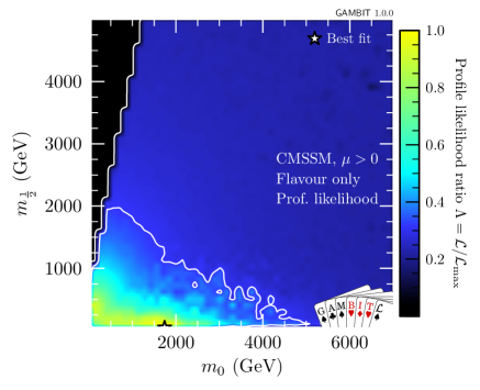
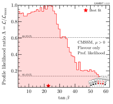
Figure 1: 2D (upper) and 1D (lower) profile likelihoods of Lagrangian parameters $m_{0}$, $m_{1/2}$ and $\tan\beta$ in a CMSSM fit including flavour and nuisance likelihoods only. Stars identify the best fit, and contours indicate 1 and $2\sigma$ confidence regions. The jagged edge of the $2\sigma$ contour at low $m_{0}$ and large $m_{1/2}$ is a plotting artefact, caused by interaction of the binning required for plotting and the abruptness of the dropoff of the likelihood in this region (due to the requirement that the lightest supersymmetric particle be a neutralino).

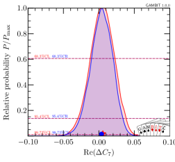
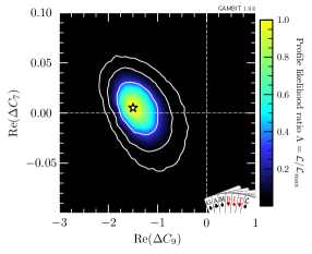
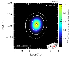
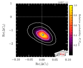
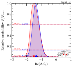
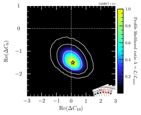
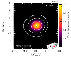
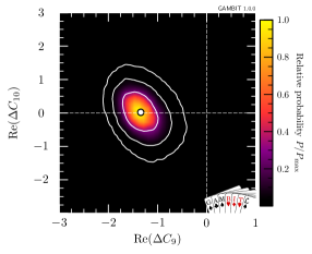
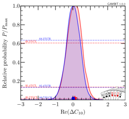
Figure 2: Profile likelihoods (upper right panels) and posterior probabilities (bottom left panels) from a scan over the real parts of the Wilson coefficients $C_{7}$, $C_{9}$ and $C_{10}$, expressed in terms of the offsets $\Delta C_{i}$ from the SM values. The central diagonal shows both 1D posterior probabilities (blue) and profile likelihoods (red) for each parameter. Stars indicate the location of the best fit, filled circles indicate posterior means, and contours correspond to 1, 2, and $3\sigma$ confidence. The SM prediction lies at the intersection of the dashed lines in the 2D panels.

In this example scan, we include the FlavBit rare leptonic and semileptonic (SL_LL), electroweak penguin (b2sll_LL), rare purely leptonic (b2ll_LL) and rare radiative likelihoods (b2sgamma_LL). In the interests of speed, numerical stability and comparability to the main CMSSM results presented in Ref. CMSSM , we do not include the prediction of $\Delta M_{s}$ from FeynHiggs nor the resulting $B$ mass asymmetry likelihood (deltaMB_LL). We employ nuisance likelihoods from PrecisionBit SDPBit to constrain $\alpha_{s}$ and $m_{t}$.

We focus specifically on the frequentist profile likelihood in this scan, and therefore employ differential evolution to sample the parameter space, as implemented in Diver ScannerBit . Consistent with Ref. CMSSM , we choose a population of 19200 and a convergence threshold of $10^{-5}$. Although the profile likelihood is in principle independent of the chosen sampling method and prior, in practice these have an impact on the sampling efficiency and the ability of a scan to uncover more isolated likelihood modes Akrami09 ; SBSpike ; ScannerBit . Our scans employ effectively logarithmic priors on the dimensionful BSM parameters, and flat priors on all other parameters. The SM parameters are sufficiently well constrained that the prior is irrelevant. We discuss the impact of the sampling prior on the BSM parameters below.

The resulting scan took approximately 15 minutes to run on 1200 CPU cores, and produced 1.1 million likelihood samples.

The results are shown in Fig. 1, in terms of the 2D profile likelihood of the sparticle masses $m_{0}$ and $m_{\frac{1}{2}}$, and the 1D profile likelihood of $\tan\beta$. The flavour likelihoods have the most impact at large $\tan\beta$, as has been extensively pointed out in the literature (e.g. Arbey:2012ax ; Mahmoudi:2014mja ). The 2D figure shows a weak preference (at the 1–2$\sigma$ level) for lower sparticle masses. At first glance this may seem surprising, given the lack of hints for SUSY, the fact that the likelihood at large $m_{0}$ and $m_{\frac{1}{2}}$ essentially recovers the SM result, and the resulting tendency of $b\rightarrow s\gamma$ to drive SUSY fits to larger masses to avoid spoiling the good agreement between the SM prediction and the observed value of $\mathcal{B}(B\rightarrow X_{s}\gamma)$. Indeed, the likelihood improvement at low mass is driven entirely by the angular analysis of $B^{0}\rightarrow K^{*}\mu^{+}\mu^{-}$ decays, with the fit attempting to account for the deviation from the SM prediction in this channel by making the new states light and boosting the (generally small) SUSY contributions as much as possible. This effect is rather small, providing an improvement in the likelihood contribution from $B^{0}\rightarrow K^{*}\mu^{+}\mu^{-}$ (b2sll_likelihood) of $\Delta\ln\mathcal{L}=3.4$ relative to the SM. This improvement is mostly counteracted by a corresponding decrease of $\Delta\ln\mathcal{L}=-2.0$ in the likelihood associated with $\mathcal{B}(B\rightarrow X_{s}\gamma)$ (b2sgamma_likelihood).

6.2 Wilson coefficient fit

As a more advanced example, we carry out a joint fit to the real parts of the $C_{7}$, $C_{9}$ and $C_{10}$ effective couplings of Eq. 2, expressed in terms of offsets from their SM values $\Delta C_{i}\equiv C_{i}-C_{i,\text{SM}}$. The YAML file for this scan can be found at yaml_files/WC.yaml.

In this example, we use the electroweak penguin likelihood (b2sll_likelihood), the rare purely leptonic decay likelihood (b2ll_likelihood) and the rare radiative decay likelihood (b2sgamma_likelihood). The other two likelihood functions available in FlavBit (based on the $B$ meson mass asymmetry and tree-level leptonic and semi-leptonic decays) have no dependence on the three Wilson coefficients that we vary. We also scan over the $\overline{MS}$ $b$ quark mass and the strong coupling as nuisance parameters, computing associated nuisance likelihoods with PrecisionBit SDPBit . We sample the parameter space with nested sampling Skilling04 ; MultiNest , using 20 000 live points and a tolerance of 0.1; see Ref. ScannerBit for details of the scanning setup and sampling algorithm.

The results of this scan are shown in Fig 2. Here we show both Bayesian posterior probabilities (lower left panels) and frequentist profile likelihoods (upper right panels), which are in rather close agreement. The small offset between the peaks of the posterior and the profile likelihood in $\Delta C_{9}$ is a volume effect, reflecting the fact that the posterior is slightly broader in $C_{7}$ and $C_{10}$ at values below the best-fit $\Delta C_{9}$ than above it. The results show a $>3\sigma$ preference for a negative offset to the muonic version of the $C_{9}$ Wilson coefficient compared to the SM, consistent with recent results from other groups Hurth:2014vma ; Altmannshofer:2017fio ; Descotes-Genon:2015uva . These are largely driven by the $B^{0}\rightarrow K^{*}\mu^{+}\mu^{-}$ angular observables, with the corresponding component of the best-fit likelihood improved by $\Delta\ln\mathcal{L}=13.2$ with respect to the SM, and $\Delta\ln\mathcal{L}=9.8$ compared to the CMSSM. We can also see that $C_{7}$ is strongly constrained by $b\rightarrow s\gamma$ decays, to within $+0.04$/$-0.03$ of its SM value.

6.3 FlavBit standalone example

GAMBIT modules can also be called directly from other codes as libraries, without actually needing to use GAMBIT itself. To do this, the calling code must specify the physics model and parameter set to be used, the module and backend functions to be run, and any required options. The calling code is responsible for resolving the dependencies and backend requirements of each module function; this is typically done “by hand” by the author of the calling code, using simple GAMBIT utility functions to hardcode the links between the chosen module and backend functions. More details of using GAMBIT modules in this so-called ‘standalone mode’ can be found in Ref. gambit .

An annotated driver program for calling FlavBit from outside the GAMBIT framework can be found in FlavBit/examples/FlavBit_standalone_example.cpp. As input, this program takes an SLHA file corresponding to the output of a spectrum generator (i.e. containing pole masses, $\overline{DR}$ parameters, etc). The name of this file can be given as a command-line argument. The program then calculates the full menu of FlavBit observables using SuperIso 3.6 and FeynHiggs 2.11.3, and uses them to calculate the five independent FlavBit likelihoods. Much of this short program is dedicated to resolving module function dependencies and backend requirements. This includes defining a local function that creates a GAMBIT Spectrum object from the input SLHA file, and others that fulfil the dependencies of SI_fill on the widths of the $Z$ and $W$ bosons.

If the user does not give the name of an input SLHA file when invoking the standalone example, it will read a default file given in the line

⬇

std::string infile("FlavBit/data/example.slha");

The likelihoods are retrieved in the lines

⬇

loglike = b2ll_likelihood(0);

loglike = b2sll_likelihood(0);

loglike = SL_likelihood(0);

loglike = b2sgamma_likelihood(0);

loglike = deltaMs_likelihood(0);

and can be combined or used for further analysis as the user requires.

The values of the observables, as used by the likelihoods, can be obtained directly from the respective observable functions in a similar manner, e.g.

⬇

double bsg = SI_bsgamma(0);

double Btaunu = SI_Btaunu(0);

and so on for all observables in Tables 1, 2 and 3.

7 Conclusions

In this paper we have described FlavBit, the flavour physics module of the public global-fitting framework GAMBIT. FlavBit provides calculations of a wide range of observables in flavour physics, ranging from tree-level decays of $B$ and $D$ mesons, to electroweak penguin decays, rare purely leptonic $B$ decays, $b\rightarrow s\gamma$ transitions, neutral meson oscillations, kaon and pion decays, and various isospin and forward-backward asymmetries. These are so far implemented for supersymmetric and effective field theories, with the list of available theories expected to grow rapidly. FlavBit also features detailed experimental data, uncertainties, correlations and likelihood functions for tree-level leptonic and semileptonic, electroweak penguin, rare purely leptonic and $B\rightarrow X_{s}\gamma$ decays, as well as for the $B^{0}_{s}$–$\bar{B}^{0}_{s}$ mass difference.

We gave a number of interesting examples of FlavBit in action. These include a standalone example program that runs FlavBit without GAMBIT, in order to compute flavour observables in supersymmetry from an input SLHA file. We carried out an example supersymmetric flavour fit with FlavBit in GAMBIT, illustrating the impacts of its likelihoods. Finally, we performed a fit to a number of observables in the context of an effective theory of flavour, demonstrating about a $4\sigma$ preference from combined experimental data for an approximately $25\%$ deficit in the (muonic) $C_{9}$ Wilson coefficient, compared to the Standard Model prediction.

The FlavBit source code can be freely downloaded from gambit.hepforge.org, either as part of GAMBIT, or as a standalone package.

Appendix A Glossary

Here we explain some terms that have specific technical definitions in GAMBIT.

backend

An external code containing useful functions (or variables) that one might wish to call (or read/write) from a module function.

backend function

A function contained in a backend. It calculates a specific quantity indicated by its capability. Its capability and call signature are defined in the backend’s frontend header.

backend requirement

A declaration that a given module function needs to be able to call a backend function or use a backend variable, identified according to its capability and type(s). Backend requirements are declared in module functions’ entries in rollcall headers.

backend variable

A global variable contained in a backend. It corresponds to a specific quantity indicated by its capability. Its capability and type are defined in the backend’s frontend header.

capability

A name describing the actual quantity that is calculated by a module or backend function. This is one possible place for units to be noted; the other is in the documented description of the capability (see Sec. 10.7 of Ref. gambit ).

dependency

A declaration that a given module function needs to be able to access the result of another module function, identified according to its capability and type. Dependencies are declared in module functions’ entries in rollcall headers.

dependency resolution

The process by which GAMBIT determines the module functions, backend functions and backend variables needed and allowed for a given scan, connects them to each others’ dependencies and backend requirements, and determines the order in which they must be called.

frontend

The interface between GAMBIT and a given backend, consisting of a frontend header plus optional source files and type headers.

frontend header

The C++ header in which the frontend to a given backend is declared.

module

A subset of GAMBIT functions following a common theme, able to be compiled into a standalone library. Although module often gets used as shorthand for physics module, this term technically also includes the GAMBIT scanning module ScannerBit.

module function

A function contained in a physics module. It calculates a specific quantity indicated by its capability and type, as declared in the module’s rollcall header. It takes only one argument, by reference (the quantity to be calculated), and has a void return type.

physics module

Any module other than ScannerBit, containing a collection of module functions following a common physics theme.

rollcall header

The C++ header in which a given physics module and its module functions are declared.

type

A general fundamental or derived C++ type, often referring to the type of the capability of a module function.

References

- (1) N. Serra, R. Silva Coutinho, and D. van Dyk, Measuring the breaking of lepton flavor universality in , Phys. Rev. D 95 (2017) 035029, [arXiv:1610.08761].
- (2) D. Straub, flav-io/flavio v0.20.3, 2017. https://doi.org/10.5281/zenodo.438351.
- (3) e. L.Silvestrini, HEPfit: a Code for the Combination of Indirect and Direct Constraints on High Energy Physics Models, 2017. .
- (4) GAMBIT Collaboration: P. Athron, C. Balazs, et. al., GAMBIT: The Global and Modular Beyond-the-Standard-Model Inference Tool, Eur. Phys. J. C in press (2017) [arXiv:1705.07908].
- (5) F. Mahmoudi, SuperIso: A Program for calculating the isospin asymmetry of in the MSSM, Comp. Phys. Comm. 178 (2008) 745, [arXiv:0710.2067].
- (6) F. Mahmoudi, SuperIso v2.3: A Program for calculating flavor physics observables in Supersymmetry, Comp. Phys. Comm. 180 (2009) 1579, [arXiv:0808.3144].
- (7) F. Mahmoudi, SuperIso v3.0, flavor physics observables calculations: Extension to NMSSM, Comp. Phys. Comm. 180 (2009) 1718.
- (8) GAMBIT Scanner Workgroup: G. D. Martinez, J. McKay, et. al., Comparison of statistical sampling methods with ScannerBit, the GAMBIT scanning module, Eur. Phys. J. C in press (2017) [arXiv:1705.07959].
- (9) GAMBIT Collaboration: P. Athron, C. Balázs, et. al., Status of the scalar singlet dark matter model, Eur. Phys. J. C 77 (2017) 568, [arXiv:1705.07931].
- (10) GAMBIT Collaboration: P. Athron, C. Balázs, et. al., Global fits of GUT-scale SUSY models with GAMBIT, Eur. Phys. J. C in press (2017) [arXiv:1705.07935].
- (11) GAMBIT Collaboration: P. Athron, C. Balázs, et. al., A global fit of the MSSM with GAMBIT, Eur. Phys. J. C in press (2017) [arXiv:1705.07917].
- (12) GAMBIT Collider Workgroup: C. Balázs, A. Buckley, et. al., ColliderBit: a GAMBIT module for the calculation of high-energy collider observables and likelihoods, Eur. Phys. J. C in press (2017) [arXiv:1705.07919].
- (13) GAMBIT Dark Matter Workgroup: T. Bringmann, J. Conrad, et. al., DarkBit: A GAMBIT module for computing dark matter observables and likelihoods, Eur. Phys. J. C in press (2017) [arXiv:1705.07920].
- (14) GAMBIT Models Workgroup: P. Athron, C. Balázs, et. al., SpecBit, DecayBit and PrecisionBit: GAMBIT modules for computing mass spectra, particle decay rates and precision observables, submitted to Eur. Phys. J. C (2017) [arXiv:1705.07936].
- (15) LHCb Collaboration: R. Aaij et. al., Angular analysis and differential branching fraction of the decay , JHEP 09 (2015) 179, [arXiv:1506.08777].
- (16) LHCb Collaboration: R. Aaij et. al., Measurement of the ratio of branching fractions , Phys. Rev. Lett. 115 (2015) 111803, [arXiv:1506.08614]. [Addendum: Phys. Rev. Lett. 115, no.15, 159901 (2015)].
- (17) LHCb Collaboration: R. Aaij et. al., Test of lepton universality using decays, Phys. Rev. Lett. 113 (2014) 151601, [arXiv:1406.6482].
- (18) LHCb Collaboration: R. Aaij et. al., Measurement of Form-Factor-Independent Observables in the Decay , Phys. Rev. Lett. 111 (2013) 191801, [arXiv:1308.1707].
- (19) BaBar Collaboration: J. P. Lees et. al., Evidence for an excess of decays, Phys. Rev. Lett. 109 (2012) 101802, [arXiv:1205.5442].
- (20) BaBar Collaboration: J. P. Lees et. al., Measurement of an Excess of Decays and Implications for Charged Higgs Bosons, Phys. Rev. D 88 (2013) 072012, [arXiv:1303.0571].
- (21) Belle Collaboration: M. Huschle et. al., Measurement of the branching ratio of relative to decays with hadronic tagging at Belle, Phys. Rev. D 92 (2015) 072014, [arXiv:1507.03233].
- (22) Belle Collaboration: A. Abdesselam et. al., Measurement of the branching ratio of relative to decays with a semileptonic tagging method, arXiv:1603.06711.
- (23) Belle Collaboration: A. Abdesselam et. al., Angular analysis of , in Proceedings, LHCSki 2016 - A First Discussion of 13 TeV Results: Obergurgl, Austria, April 10-15, 2016 (2016) [arXiv:1604.04042].
- (24) M. Cacciari, G. P. Salam, and G. Soyez, FastJet User Manual, Eur. Phys. J. C 72 (2012) 1896, [arXiv:1111.6097].
- (25) P. Athron, J.-h. Park, D. Stöckinger, and A. Voigt, FlexibleSUSY - A spectrum generator generator for supersymmetric models, Comp. Phys. Comm. 190 (2015) 139–172, [arXiv:1406.2319].
- (26) B. C. Allanach, SOFTSUSY: a program for calculating supersymmetric spectra, Comp. Phys. Comm. 143 (2002) 305–331, [hep-ph/0104145].
- (27) S. Heinemeyer, W. Hollik, and G. Weiglein, FeynHiggs: A Program for the calculation of the masses of the neutral CP even Higgs bosons in the MSSM, Comp. Phys. Comm. 124 (2000) 76–89, [hep-ph/9812320].
- (28) Particle Data Group: C. Patrignani et. al., Review of Particle Physics, Chin. Phys. C40 (2016) 100001.
- (29) Y. Sakaki, M. Tanaka, A. Tayduganov, and R. Watanabe, Testing leptoquark models in , Phys. Rev. D 88 (2013) 094012, [arXiv:1309.0301].
- (30) A. Crivellin, J. Heeck, and P. Stoffer, A perturbed lepton-specific two-Higgs-doublet model facing experimental hints for physics beyond the Standard Model, Phys. Rev. Lett. 116 (2016) 081801, [arXiv:1507.07567].
- (31) M. Freytsis, Z. Ligeti, and J. T. Ruderman, Flavor models for , Phys. Rev. D 92 (2015) 054018, [arXiv:1506.08896].
- (32) A. J. Buras and J. Girrbach, Towards the Identification of New Physics through Quark Flavour Violating Processes, Rep. Prog. Phys. 77 (2014) 086201, [arXiv:1306.3775].
- (33) O. Eberhardt, U. Nierste, and M. Wiebusch, Status of the two-Higgs-doublet model of type II, JHEP 07 (2013) 118, [arXiv:1305.1649].
- (34) D. Das, C. Hati, G. Kumar, and N. Mahajan, Towards a unified explanation of , and anomalies in a L-R model, arXiv:1605.06313.
- (35) A. Greljo, G. Isidori, and D. Marzocca, On the breaking of Lepton Flavor Universality in B decays, JHEP 07 (2015) 142, [arXiv:1506.01705].
- (36) S. M. Boucenna, A. Celis, J. Fuentes-Martin, A. Vicente, and J. Virto, Phenomenology of an model with lepton-flavour non-universality, arXiv:1608.01349.
- (37) D. Becirevic, N. Kosnik, O. Sumensari, and R. Zukanovich Funchal, Palatable Leptoquark Scenarios for Lepton Flavor Violation in Exclusive modes, arXiv:1608.07583.
- (38) I. Dorsner, S. Fajfer, A. Greljo, J. F. Kamenik, and N. Kosnik, Physics of leptoquarks in precision experiments and at particle colliders, Phys. Rep. 641 (2016) 1–68, [arXiv:1603.04993].
- (39) UTfit Collaboration: M. Bona et. al., An Improved Standard Model Prediction Of BR() And Its Implications For New Physics, Phys. Lett. B 687 (2010) 61–69, [arXiv:0908.3470].
- (40) A. G. Akeroyd and F. Mahmoudi, Constraints on charged Higgs bosons from and , JHEP 04 (2009) 121, [arXiv:0902.2393].
- (41) M. Beneke, T. Feldmann, and D. Seidel, Systematic approach to exclusive , decays, Nucl. Phys. B 612 (2001) 25–58, [hep-ph/0106067].
- (42) C. Greub, A. Ioannisian, and D. Wyler, Effects of new physics in the rare decays and , Phys. Lett. B 346 (1995) 149–158, [hep-ph/9408382].
- (43) F. Kruger and L. M. Sehgal, Lepton polarization in the decays and , Phys. Lett. B 380 (1996) 199–204, [hep-ph/9603237].
- (44) G. Hiller and F. Kruger, More model independent analysis of processes, Phys. Rev. D 69 (2004) 074020, [hep-ph/0310219].
- (45) LHCb Collaboration: R. Aaij et. al., Differential branching fraction and angular analysis of the decay , JHEP 08 (2013) 131, [arXiv:1304.6325].
- (46) J. Gratrex, M. Hopfer, and R. Zwicky, Generalised helicity formalism, higher moments and the angular distributions, Phys. Rev. D 93 (2016) 054008, [arXiv:1506.03970].
- (47) LHCb Collaboration: R. Aaij et. al., Angular analysis of the decay using 3 fb-1 of integrated luminosity, JHEP 02 (2016) 104, [arXiv:1512.04442].
- (48) F. Beaujean, M. Chrząszcz, N. Serra, and D. van Dyk, Extracting Angular Observables without a Likelihood and Applications to Rare Decays, Phys. Rev. D 91 (2015) 114012, [arXiv:1503.04100].
- (49) W. Altmannshofer, P. Ball, et. al., Symmetries and Asymmetries of Decays in the Standard Model and Beyond, JHEP 01 (2009) 019, [arXiv:0811.1214].
- (50) S. Descotes-Genon, T. Hurth, J. Matias, and J. Virto, Optimizing the basis of observables in the full kinematic range, JHEP 05 (2013) 137, [arXiv:1303.5794].
- (51) F. Kruger and J. Matias, Probing new physics via the transverse amplitudes of at large recoil, Phys. Rev. D 71 (2005) 094009, [hep-ph/0502060].
- (52) D. Becirevic and E. Schneider, On transverse asymmetries in , Nucl. Phys. B 854 (2012) 321–339, [arXiv:1106.3283].
- (53) A. Bharucha, D. M. Straub, and R. Zwicky, in the Standard Model from light-cone sum rules, JHEP 08 (2016) 098, [arXiv:1503.05534].
- (54) S. Jäger and J. Martin Camalich, On at small dilepton invariant mass, power corrections, and new physics, JHEP 05 (2013) 043, [arXiv:1212.2263].
- (55) J. Lyon and R. Zwicky, Resonances gone topsy turvy - the charm of QCD or new physics in ?, arXiv:1406.0566.
- (56) M. Ciuchini, M. Fedele, et. al., decays at large recoil in the Standard Model: a theoretical reappraisal, JHEP 06 (2016) 116, [arXiv:1512.07157].
- (57) V. G. Chobanova, T. Hurth, F. Mahmoudi, D. Martinez Santos, and S. Neshatpour, Large hadronic power corrections or new physics in the rare decay ?, JHEP 07 (2017) 025, [arXiv:1702.02234].
- (58) S. Descotes-Genon, J. Matias, and J. Virto, Understanding the Anomaly, Phys. Rev. D 88 (2013) 074002, [arXiv:1307.5683].
- (59) W. Altmannshofer and D. M. Straub, New physics in ?, Eur. Phys. J. C 73 (2013) 2646, [arXiv:1308.1501].
- (60) T. Hurth and F. Mahmoudi, On the LHCb anomaly in , JHEP 04 (2014) 097, [arXiv:1312.5267].
- (61) S. Jäger and J. Martin Camalich, Reassessing the discovery potential of the decays in the large-recoil region: SM challenges and BSM opportunities, Phys. Rev. D 93 (2016) 014028, [arXiv:1412.3183].
- (62) T. Hurth, F. Mahmoudi, and S. Neshatpour, On the anomalies in the latest LHCb data, Nucl. Phys. B 909 (2016) 737–777, [arXiv:1603.00865].
- (63) LHCb Collaboration: R. Aaij et. al., Angular analysis of the decay in the low-q2 region, JHEP 04 (2015) 064, [arXiv:1501.03038].
- (64) T. Feldmann and J. Matias, Forward-backward and isospin asymmetry for decay in the standard model and in supersymmetry, JHEP 1 (2003) 074, [hep-ph/0212158].
- (65) T. Huber, T. Hurth, and E. Lunghi, Inclusive : complete angular analysis and a thorough study of collinear photons, JHEP 06 (2015) 176, [arXiv:1503.04849].
- (66) BaBar Collaboration: B. Aubert et. al., Measurement of the branching fraction with a sum over exclusive modes, Phys. Rev. Lett. 93 (2004) 081802, [hep-ex/0404006].
- (67) Belle Collaboration: M. Iwasaki et. al., Improved measurement of the electroweak penguin process , Phys. Rev. D 72 (2005) 092005, [hep-ex/0503044].
- (68) Belle Collaboration: Y. Sato et. al., Measurement of the lepton forward-backward asymmetry in decays with a sum of exclusive modes, Phys. Rev. D 93 (2016) 032008, [arXiv:1402.7134]. [Addendum: Phys. Rev. D93, no.5, 059901 (2016)].
- (69) BaBar Collaboration: J. P. Lees et. al., Measurement of the branching fraction and search for direct CP violation from a sum of exclusive final states, Phys. Rev. Lett. 112 (2014) 211802, [arXiv:1312.5364].
- (70) LHCb Collaboration: R. Aaij et. al., Differential branching fraction and angular moments analysis of the decay in the region, JHEP 12 (2016) 065, [arXiv:1609.04736].
- (71) D. Das, G. Hiller, M. Jung, and A. Shires, The and distributions at low hadronic recoil, JHEP 09 (2014) 109, [arXiv:1406.6681].
- (72) F. Mahmoudi, S. Neshatpour, and J. Virto, optimised observables in the MSSM, Eur. Phys. J. C 74 (2014) 2927, [arXiv:1401.2145].
- (73) S. Bertolini, F. Borzumati, A. Masiero, and G. Ridolfi, Effects of supergravity induced electroweak breaking on rare decays and mixings, Nucl. Phys. B353 (1991) 591–649.
- (74) M. Misiak et. al., Estimate of at , Phys. Rev. Lett. 98 (2007) 022002, [hep-ph/0609232].
- (75) F. Mahmoudi and O. Stål, Flavor constraints on the two-Higgs-doublet model with general Yukawa couplings, Phys. Rev. D 81 (2010) 035016, [arXiv:0907.1791].
- (76) T. Hermann, M. Misiak, and M. Steinhauser, in the Two Higgs Doublet Model up to Next-to-Next-to-Leading Order in QCD, JHEP 11 (2012) 036, [arXiv:1208.2788].
- (77) M. Misiak et. al., Updated NNLO QCD predictions for the weak radiative -meson decays, Phys. Rev. Lett. 114 (2015) 221801, [arXiv:1503.01789].
- (78) M. Misiak and M. Steinhauser, Weak Radiative Decays of the B Meson and Bounds on in the Two-Higgs-Doublet Model, Eur. Phys. J. C 77 (2017) 201, [arXiv:1702.04571].
- (79) A. L. Kagan and M. Neubert, QCD anatomy of B —> X(s gamma) decays, Eur. Phys. J. C 7 (1999) 5–27, [hep-ph/9805303].
- (80) A. L. Kagan and M. Neubert, Isospin breaking in decays, Phys. Lett. B539 (2002) 227–234, [hep-ph/0110078].
- (81) M. R. Ahmady and F. Mahmoudi, Constraints on the mSUGRA parameter space from NLO calculation of isospin asymmetry in , Phys. Rev. D 75 (2007) 015007, [hep-ph/0608212].
- (82) M. González-Alonso and J. Martin Camalich, Global Effective-Field-Theory analysis of New-Physics effects in (semi)leptonic kaon decays, JHEP 12 (2016) 052, [arXiv:1605.07114].
- (83) FlaviaNet Working Group on Kaon Decays: M. Antonelli et. al., Precision tests of the Standard Model with leptonic and semileptonic kaon decays, in PHIPSI08, proceedings of the International Workshop on Collisions from phi to psi, Frascati (Rome) Italy, 7-10 April 2008 (2008) [arXiv:0801.1817].
- (84) A. J. Buras, P. H. Chankowski, J. Rosiek, and L. Slawianowska, and in supersymmetry at large , Nucl. Phys. B659 (2003) 3, [hep-ph/0210145].
- (85) BaBar Collaboration: B. Aubert et. al., A Measurement of the branching fractions of exclusive () ( decays in events with a fully reconstructed meson, Phys. Rev. Lett. 100 (2008) 151802, [arXiv:0712.3503].
- (86) BaBar Collaboration: B. Aubert et. al., Measurement of |V(cb)| and the Form-Factor Slope in anti-B —> D l- anti-nu Decays in Events Tagged by a Fully Reconstructed B Meson, Phys. Rev. Lett. 104 (2010) 011802, [arXiv:0904.4063].
- (87) Belle Collaboration: W. Dungel et. al., Measurement of the form factors of the decay and determination of the CKM matrix element |Vcb|, Phys. Rev. D 82 (2010) 112007, [arXiv:1010.5620].
- (88) Belle Collaboration: R. Glattauer et. al., Measurement of the decay in fully reconstructed events and determination of the Cabibbo-Kobayashi-Maskawa matrix element , Phys. Rev. D 93 (2016) 032006, [arXiv:1510.03657].
- (89) Belle Collaboration: Y. Sato et. al., Measurement of the branching ratio of relative to decays with a semileptonic tagging method, Phys. Rev. D 94 (2016) 072007, [arXiv:1607.07923].
- (90) Belle Collaboration: S. Hirose et. al., Measurement of the lepton polarization and in the decay , arXiv:1612.00529.
- (91) Y. Amhis et. al., Averages of -hadron, -hadron, and -lepton properties as of summer 2016, arXiv:1612.07233.
- (92) Y. Amhis et. al., Average of and for Moriond EW 2017, http://www.slac.stanford.edu/ xorg/hfag/semi/moriond17/RDRDs.html.
- (93) HPQCD Collaboration: H. Na, C. M. Bouchard, G. P. Lepage, C. Monahan, and J. Shigemitsu, form factors at nonzero recoil and extraction of , Phys. Rev. D 92 (2015) 054510, [arXiv:1505.03925]. [Erratum: Phys. Rev. D93, no.11, 119906 (2016)].
- (94) S. Fajfer, J. F. Kamenik, and I. Nisandzic, On the Sensitivity to New Physics, Phys. Rev. D 85 (2012) 094025, [arXiv:1203.2654].
- (95) S. Fajfer, J. F. Kamenik, and I. Nišandžić, , Phys. Rev. D 85 (2012) 094025.
- (96) Fermilab Lattice, MILC: J. A. Bailey et. al., from decays and (2+1)-flavor lattice QCD, Phys. Rev. D 92 (2015) 014024, [arXiv:1503.07839].
- (97) BaBar Collaboration: J. P. Lees et. al., Evidence of decays with hadronic B tags, Phys. Rev. D 88 (2013) 031102, [arXiv:1207.0698].
- (98) BaBar Collaboration: B. Aubert et. al., A Search for Recoiling Against , Phys. Rev. D 81 (2010) 051101, [arXiv:0912.2453].
- (99) Belle Collaboration: I. Adachi et. al., Evidence for with a Hadronic Tagging Method Using the Full Data Sample of Belle, Phys. Rev. Lett. 110 (2013) 131801, [arXiv:1208.4678].
- (100) Belle Collaboration: K. Hara et. al., Evidence for with a Semileptonic Tagging Method, Phys. Rev. D 82 (2010) 071101, [arXiv:1006.4201].
- (101) ATLAS Collaboration, Angular analysis of decays in collisions at TeV with the ATLAS detector, in 52nd Rencontres de Moriond on Electroweak Interactions and Unified Theories (2017) ATLAS-CONF-2017-023.
- (102) CMS Collaboration, Measurement of the and angular parameters of the decay in proton-proton collisions at , in 52nd Rencontres de Moriond on Electroweak Interactions and Unified Theories (2017) CMS-PAS-BPH-15-008.
- (103) F. Mahmoudi, T. Hurth, and S. Neshatpour, Present Status of Anomalies, in 6th Workshop on Theory, Phenomenology and Experiments in Flavour Physics: Interplay of Flavour Physics with electroweak symmetry breaking (Capri 2016) Anacapri, Capri, Italy, June 11, 2016 (2016) [arXiv:1611.05060].
- (104) LHCb Collaboration: R. Aaij et. al., Measurement of the branching fraction and effective lifetime and search for decays, arXiv:1703.05747.
- (105) LHCb & CMS Collaborations: V. Khachatryan et. al., Observation of the rare decay from the combined analysis of CMS and LHCb data, Nature 522 (2015) 68–72, [arXiv:1411.4413].
- (106) LHCb Collaboration: R. Aaij et. al., Measurement of the branching fraction and search for decays at the LHCb experiment, Phys. Rev. Lett. 111 (2013) 101805, [arXiv:1307.5024].
- (107) CMS Collaboration: S. Chatrchyan et. al., Measurement of the branching fraction and search for with the CMS Experiment, Phys. Rev. Lett. 111 (2013) 101804, [arXiv:1307.5025].
- (108) ATLAS Collaboration: M. Aaboud et. al., Study of the rare decays of and into muon pairs from data collected during the LHC Run 1 with the ATLAS detector, arXiv:1604.04263.
- (109) CDF Collaboration: T. Aaltonen et. al., Search for the Decays and in CDF Run II, Phys. Rev. Lett. 102 (2009) 201801, [arXiv:0901.3803].
- (110) LHCb Collaboration: R. Aaij et. al., Search for the decays and , arXiv:1703.02508.
- (111) BaBar Collaboration: B. Aubert et. al., A search for the rare decay at BABAR, Phys. Rev. Lett. 96 (2006) 241802, [hep-ex/0511015].
- (112) A. J. Buras, J. Girrbach, D. Guadagnoli, and G. Isidori, On the Standard Model prediction for BR(), Eur. Phys. J. C 72 (2012) 2172, [arXiv:1208.0934].
- (113) BaBar Collaboration: B. Aubert et. al., Measurement of the branching fraction and photon energy spectrum using the recoil method, Phys. Rev. D 77 (2008) 051103, [arXiv:0711.4889].
- (114) BaBar Collaboration: J. P. Lees et. al., Exclusive Measurements of Transition Rate and Photon Energy Spectrum, Phys. Rev. D 86 (2012) 052012, [arXiv:1207.2520].
- (115) BaBar Collaboration: J. P. Lees et. al., Precision Measurement of the Photon Energy Spectrum, Branching Fraction, and Direct CP Asymmetry , Phys. Rev. Lett. 109 (2012) 191801, [arXiv:1207.2690].
- (116) Belle Collaboration: T. Saito et. al., Measurement of the Branching Fraction with a Sum of Exclusive Decays, Phys. Rev. D 91 (2015) 052004, [arXiv:1411.7198].
- (117) Belle Collaboration: A. Abdesselam et. al., Measurement of the inclusive branching fraction, photon energy spectrum and HQE parameters, in Proceedings, 38th International Conference on High Energy Physics (ICHEP 2016): Chicago, IL, USA, August 3-10, 2016 (2016) [arXiv:1608.02344].
- (118) M. Czakon, P. Fiedler, et. al., The contribution to at , JHEP 04 (2015) 168, [arXiv:1503.01791].
- (119) M. Artuso, G. Borissov, and A. Lenz, CP violation in the system, Rev. Mod. Phys. 88 (2016) 045002, [arXiv:1511.09466].
- (120) KLOE Collaboration: F. Ambrosino et. al., Precise measurement of and study of , Eur. Phys. J. C 64 (2009) 627–636, [arXiv:0907.3594]. [Erratum: Eur. Phys. J. C65, 703 (2010)].
- (121) NA62 Collaboration: C. Lazzeroni et. al., Precision Measurement of the Ratio of the Charged Kaon Leptonic Decay Rates, Phys. Lett. B 719 (2013) 326–336, [arXiv:1212.4012].
- (122) Y. Akrami, P. Scott, J. Edsjö, J. Conrad, and L. Bergström, A profile likelihood analysis of the Constrained MSSM with genetic algorithms, JHEP 4 (2010) 57, [arXiv:0910.3950].
- (123) F. Feroz, K. Cranmer, M. Hobson, R. Ruiz de Austri, and R. Trotta, Challenges of profile likelihood evaluation in multi-dimensional SUSY scans, JHEP 6 (2011) 42, [arXiv:1101.3296].
- (124) A. Arbey, M. Battaglia, F. Mahmoudi, and D. Martinez Santos, Supersymmetry confronts : Present and future status, Phys. Rev. D 87 (2013) 035026, [arXiv:1212.4887].
- (125) J. Skilling, Nested Sampling, in American Institute of Physics Conference Series (R. Fischer, R. Preuss, and U. V. Toussaint, eds.) 735 (2004) 395–405.
- (126) F. Feroz, M. P. Hobson, and M. Bridges, MULTINEST: an efficient and robust Bayesian inference tool for cosmology and particle physics, MNRAS 398 (2009) 1601–1614, [arXiv:0809.3437].
- (127) T. Hurth, F. Mahmoudi, and S. Neshatpour, Global fits to data and signs for lepton non-universality, JHEP 12 (2014) 053, [arXiv:1410.4545].
- (128) W. Altmannshofer, C. Niehoff, P. Stangl, and D. M. Straub, Status of the anomaly after Moriond 2017, arXiv:1703.09189.
- (129) S. Descotes-Genon, L. Hofer, J. Matias, and J. Virto, Global analysis of anomalies, JHEP 06 (2016) 092, [arXiv:1510.04239].