Abstract

The differential equation proposed by Frits Zernike to obtain a basis of polynomial orthogonal solutions on the the unit disk to classify wavefront aberrations in circular pupils, is shown to have a set of new orthonormal solution bases, involving Legendre and Gegenbauer polynomials, in non-orthogonal coordinates close to Cartesian ones. We find the overlaps between the original Zernike basis and a representative of the new set, which turn out to be Clebsch-Gordan coefficients.

1 Introduction: the Zernike system

In 1934 Frits Zernike published a paper which gave rise to phase-contrast microscopy [1]. This paper presented a differential equation of second degree to provide an orthogonal basis of polynomial solutions on the unit disk to describe wavefront aberrations in circular pupils. This basis was also obtained in Ref. [2] using the Schmidt orthogonalization process, as its authors noted that the reason to set up Zernike’s differential equation had not been clearly justified. The two-dimensional differential equation in ${\bf r}=(x,y)$ that Zernike solved is

$$\widehat{Z}\Psi{{\scriptstyle(}{\bf r}{\scriptstyle)}}:=\Big{(}\nabla^{2}-({\bf r}\cdot\nabla)^{2}-2\,{\bf r}\cdot\nabla\Big{)}\Psi{{\scriptstyle(}{\bf r}{\scriptstyle)}}=-E\,\Psi{{\scriptstyle(}{\bf r}{\scriptstyle)}},$$ (1)

on the unit disk ${\cal D}:=\{{{\scriptstyle|}{\bf r}{\scriptstyle|}}\leq 1\}$ and $\Psi{{\scriptstyle(}{\bf r}{\scriptstyle)}}\in{\cal L}^{2}({\cal D})$ (once two parameters had been fixed by the condition of self-adjointness). The solutions found by Zernike are separable in polar coordinates $(r,\phi)$, with Jacobi polynomials of degrees $n_{r}$ in the radius $r:={{\scriptstyle|}{\bf r}{\scriptstyle|}}$ times trigonometric functions $e^{{\rm i}m\phi}$ in the angle $\phi$. The solutions are thus classified by $(n_{r},m)$, which add up to non-negative integers $n=2n_{r}+{{\scriptstyle|}m{\scriptstyle|}}$, providing the quantized eigenvalues $E_{n}=n(n+2)$ for the operator in (1).

The spectrum $(n_{r},m)$ or $(n,m)$ of the Zernike system is exactly that of the two-dimensional quantum harmonic oscillator. This evident analogy with the quantum oscillator spectrum has been misleading, however. Two-term raising and lowering operators do not exist; only three-term recurrence relations have been found [3, 4, 5, 6, 7]. Beyond the rotational symmetry that explains the multiplets in $\{m\}$, no Lie algebra has been shown to explain the symmetry hidden in the equal spacing of $n$ familiar from the oscillator model.

In Refs. [8, 9] we have interpreted Zernike’s equation (1) as defining a classical and a quantum system with a non-standard ‘Hamiltonian’ $-{\textstyle\frac{1}{2}}\hat{Z}$. This turns out to be interesting because in the classical system the trajectories turn out to be closed ellipses, and in the quantum system this Hamiltonian partakes in a cubic Higgs superintegrable algebra [10].

The key to solve the system was to perform a ‘vertical’ map from the disk $\cal D$ in ${\bf r}=(x,y)$ to a half-sphere in three-space $\vec{\,r}=(x,y,z)$, to be indicated as ${\cal H}_{+}:=\{\,|\!\vec{\,r}|=1,\,z\geq 0\}$. On ${\cal H}_{+}$ the issue of separability of solutions becomes clear: the orthogonal spherical coordinate system $(\vartheta,\varphi)$, $\vartheta\in[0,{\textstyle\frac{1}{2}}\pi]$, $\varphi\in(-\pi,\pi]$ on ${\cal H}_{+}$, projects on the polar coordinates $(r,\phi)$ of $\cal D$. But as shown in Fig. 1, the half-sphere can also be covered with other orthogonal and separated coordinate systems (i.e., those whose boundary coincides with one fixed coordinate): where the coordinate poles are along the $x$-axis and the range of spherical angles is $\vartheta^{\prime}\in[0,\pi]$ and $\varphi^{\prime}\in[0,\pi]$. Since the poles of the spherical coordinates can lie in any direction of the $(x,y)$-plane and rotated around them, we take the $x$-axis orientation as representing the whole class of new solutions, which we identify by the label II, to distinguish them from Zernike’s polar-separated solutions that will be labelled I.

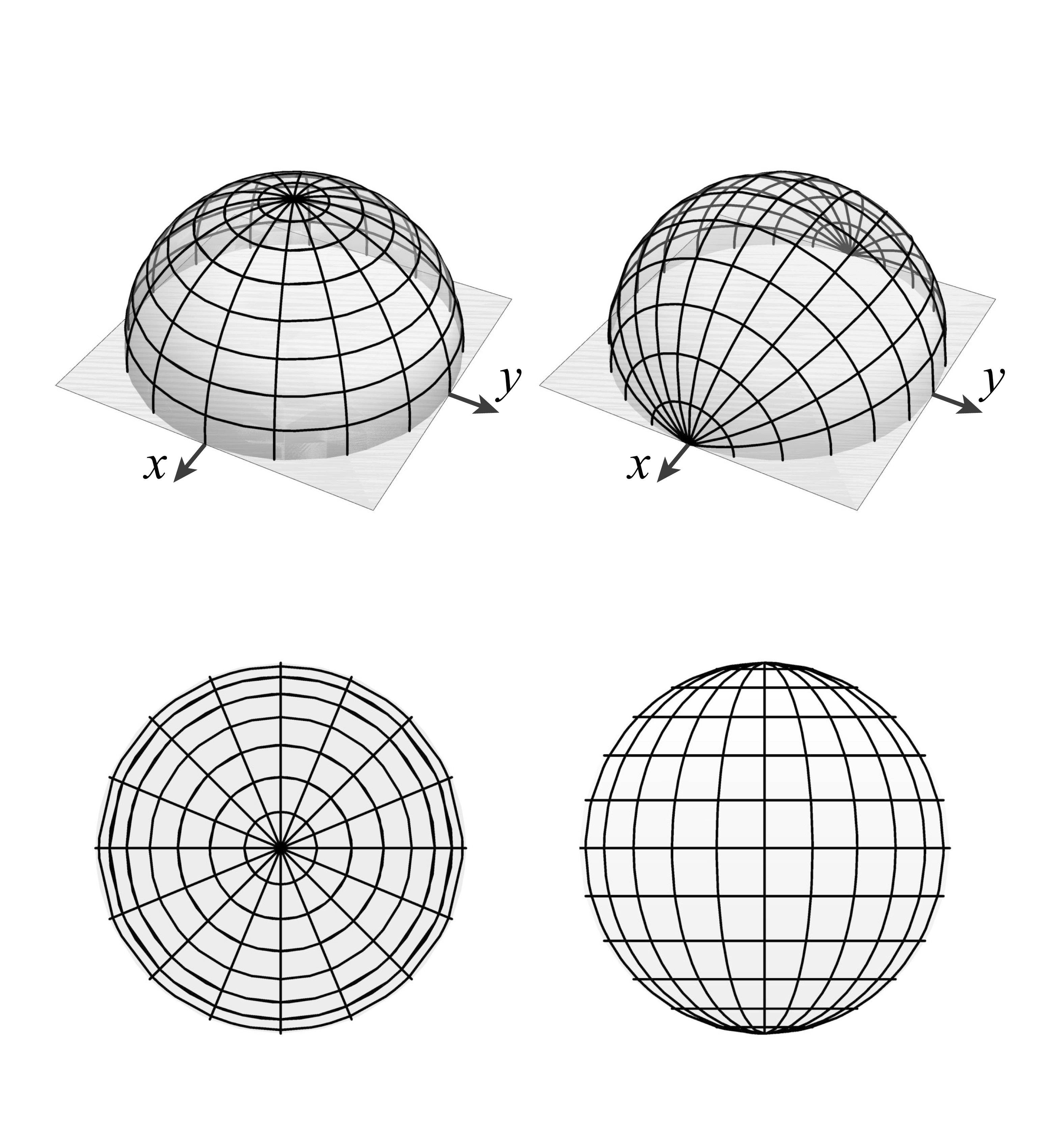
Figure 1: Top row: Orthogonal coordinate systems that separate on the half-sphere ${\cal H}_{+}$. Bottom row: Their vertical projection on the disk $\cal D$. Left: Spherical coordinates with their pole at the $+z$-axis; separated solutions will be marked by I. Right: Spherical coordinates with their pole along the $+x$-axis, whose solutions are identified by II. The latter maps on non-orthogonal coordinates on the disk that also separate solutions of the Zernike equation.

The coordinate system II is orthogonal on ${\cal H}_{+}$ but projects on non-orthogonal ones on $\cal D$; the new separated solutions consist of Legendre and Gegenbauer polynomials [9]. Of course, the spectrum $\{E_{n}\}$ in (1) is the same as in the coordinate system I. Recall also that coordinates which separate a differential equation lead to extra commuting operators and constants of the motion. In this paper we proceed to find the I-II interbasis expansions between the original Zernike and the newly found solution bases; its compact expression in terms of su($2$) Clebsch-Gordan coefficients certainly indicates that some kind of deeper symmetry is at work.

The solutions of the Zernike system [1] in the new coordinate system, that we indicate by $\Upsilon^{\scriptscriptstyle\rm I}$ and $\Upsilon^{\scriptscriptstyle\rm II}$ on ${\cal H}_{+}$, and $\Psi^{\scriptscriptstyle\rm I}$ and $\Psi^{\scriptscriptstyle\rm II}$ on ${\cal D}$, are succinctly derived and written out in Sect. 2. In Sect. 3 we find the overlap between them, add some remarks in the concluding Sect. 4, and reserve for the Appendices some special-function developments and an explicit list with the lowest-$n$ transformation matrices.

2 Two coordinate systems, two function bases

The Zernike differential equation (1) in ${\bf r}=(x,y)$ on the disk ${\cal D}$ can be ‘elevated’ to a differential equation on the half-sphere ${\cal H}_{+}$ in Fig. 1 through first defining the coordinates $\vec{\,\xi}=(\xi_{1},\xi_{2},\xi_{3})$ by

$$\xi_{1}:=x,\quad\xi_{2}:=y,\quad\xi_{3}:=\sqrt{1-x^{2}-y^{2}},$$ (2)

then relating the measures of ${\cal H}_{+}$ and $\cal D$ through

$${\rm d}^{2}S(\!\vec{\,\xi})=\frac{{\rm d}\xi_{1}\,{\rm d}\xi_{2}}{\xi_{3}}=\frac{{\rm d}x\,{\rm d}y}{\sqrt{1-x^{2}-y^{2}}}=\frac{{\rm d}^{2}{\bf r}}{\sqrt{1-{{\scriptstyle|}{\bf r}{\scriptstyle|}}^{2}}},$$ (3)

and the partial derivatives by $\partial_{x}=\partial_{\xi_{1}}-(\xi_{1}/\xi_{3})\partial_{\xi_{3}}$ and $\partial_{y}=\partial_{\xi_{2}}-(\xi_{2}/\xi_{3})\partial_{\xi_{3}}$.

2.1 Map between ${\cal H}_{+}$ and $\cal D$ operators

Due to the change in measure (3), the Zernike operator on $\cal D$, $\widehat{Z}$ in (1), must be subject to a similarity transformation by the root of the factor between ${\rm d}^{2}S(\vec{\xi})$ and ${\rm d}^{2}{\bf r}$; thus we define the Zernike operator on the half-sphere ${\cal H}_{+}$ and its solutions, as

$$\widehat{W}:=(1-{{\scriptstyle|}{\bf r}{\scriptstyle|}}^{2})^{1/4}\,\widehat{Z}\,(1-{{\scriptstyle|}{\bf r}{\scriptstyle|}}^{2})^{-1/4},\quad\Upsilon(\!\vec{\,\xi}):=(1-{{\scriptstyle|}{\bf r}{\scriptstyle|}}^{2})^{1/4}\Psi({\bf r}).$$ (4)

In this way the inner product required for functions on the disk and on the sphere are related by

$$(\Psi,\Psi^{\prime})_{\cal D}:=\int_{\cal D}{\rm d}^{2}{\bf r}\,\Psi{{\scriptstyle(}{\bf r}{\scriptstyle)}}^{*}\Psi^{\prime}{{\scriptstyle(}{\bf r}{\scriptstyle)}}=\int_{{\cal H}_{+}}{\rm d}^{2}S(\!\vec{\,\xi})\,\Upsilon(\!\vec{\,\xi})^{*}\,\Upsilon^{\prime}(\!\vec{\,\xi})=:(\Upsilon,\Upsilon^{\prime})_{{\cal H}_{+}}.$$ (5)

Perhaps rather surprisingly, the Zernike operator $\widehat{W}$ in (4) on $\vec{\,\xi}\in{\cal H}_{+}$ has the structure of ($-2$ times) a Schrödinger Hamiltonian,

$$\widehat{W}\Upsilon(\!\vec{\,\xi})=\bigg{(}\Delta_{\scriptscriptstyle\rm LB}+\frac{\xi_{1}^{2}+\xi_{2}^{2}}{4\xi_{3}^{2}}+1\bigg{)}\Upsilon(\!\vec{\,\xi})=-E\Upsilon(\!\vec{\,\xi}),$$ (6)

which is a sum of the Laplace-Beltrami operator $\Delta_{\scriptscriptstyle\rm LB}=\hat{L}^{2}_{1}+\hat{L}^{2}_{2}+\hat{L}^{2}_{3}$, where

$$\hat{L}_{1}:=\xi_{3}\partial_{\xi_{2}}-\xi_{2}\partial_{\xi_{3}},\quad\hat{L}_{2}:=\xi_{1}\partial_{\xi_{3}}-\xi_{3}\partial_{\xi_{1}},\quad\hat{L}_{3}:=\xi_{2}\partial_{\xi_{1}}-\xi_{1}\partial_{\xi_{1}},$$ (7)

are the generators of a formal so($3$) Lie algebra. The second summand in (6) represents a radial potential $V_{\scriptscriptstyle\rm\!W}{{\scriptstyle(}r{\scriptstyle)}}:=-r^{2}/8(1-r^{2})$ which has the form of a repulsive oscillator constrained to $(-1,1)$, whose rather delicate boundary conditions were addressed in Ref. [9].

The coordinates $\vec{\,\xi}$ can be now expressed in terms of the two mutually orthogonal systems of coordinates on the sphere [11] as shown in Fig. 1:

System I:

$$\hskip-30.0pt\xi_{1}=\sin\vartheta\cos\varphi,\quad\xi_{2}=\sin\vartheta\sin\varphi,\quad\xi_{3}=\cos\vartheta,\qquad\vartheta|_{0}^{\pi/2},\ \varphi|_{-\pi}^{\pi},$$ (8)

System II:

$$\hskip-30.0pt\xi_{1}=\cos\vartheta^{\prime},\quad\xi_{2}=\sin\vartheta^{\prime}\cos\varphi^{\prime},\quad\xi_{3}=\sin\vartheta^{\prime}\sin\varphi^{\prime},\qquad\vartheta^{\prime}|_{0}^{\pi},\ \varphi^{\prime}|_{0}^{\pi}.$$ (9)

In the following we succinctly give the normalized solutions for the differential equation (6) in terms of the angles for ${\cal H}_{+}$ in the coordinate systems I and II, and their projection as wavefronts on the disk $\cal D$ of the optical pupil. The spectrum of quantum numbers that classify each eigenbasis, $(n,m)$ and $(n_{1},n_{2})$, will indeed be formally identical with that of the two-dimensional quantum harmonic oscillator in polar and Cartesian coordinates, respectively.

2.2 Solutions in System I (8)

Zernike’s differential equation (1) is clearly invariant under rotations around the center of the disk, corresponding to rotations of $\widehat{W}$ in (6) around the $\xi_{3}$-axis of the coordinate system (8) on the sphere. Written out in those coordinates, it has the form of a Schrödinger equation,

$$\frac{1}{\sin\vartheta}\frac{\partial}{\partial\vartheta}\sin\vartheta\frac{\partial\Upsilon^{\scriptscriptstyle\rm I}(\vartheta,\varphi)}{\partial\vartheta}+\frac{1}{\sin^{2}\theta}\frac{\partial^{2}\Upsilon^{\scriptscriptstyle\rm I}(\vartheta,\varphi)}{\partial\varphi^{2}}+(E+{\textstyle\frac{1}{4}}\tan^{2}\vartheta+1)\Upsilon^{\scriptscriptstyle\rm I}(\vartheta,\varphi)=0,$$ (10)

with a potential $V_{\scriptscriptstyle\rm\!W}(\vartheta)=-\frac{1}{8}\tan^{2}\vartheta$. Clearly this will separate into a differential equation in $\varphi$ with a separating constant $m^{2}$, where $m\in{\cal Z}:=\{0,\pm 1,\pm 2,\ldots\}$ and solutions $\sim e^{{\rm i}m\varphi}$. This separation constant then enters into a differential equation in $\vartheta$ that has also has the form of a one-dimensional Schrödinger equation with an effective potential of the Pöschl-Teller type $V^{\scriptscriptstyle\rm I}_{\scriptscriptstyle\rm\!eff}(\vartheta)=(m^{2}-\frac{1}{4})\csc^{2}\vartheta-\frac{1}{4}\sec^{2}\vartheta$, whose solutions with the proper boundary conditions at $\vartheta={\textstyle\frac{1}{2}}\pi$ are Jacobi polynomials.

On the half-sphere the solutions to (6) are thus

$$\Upsilon^{\scriptscriptstyle\rm I}_{n,m}(\vartheta,\varphi):=\sqrt{\frac{n{+}1}{\pi}}\,(\sin\vartheta)^{{{\scriptstyle|}m{\scriptstyle|}}}\,(\cos\vartheta)^{1/2}P_{\frac{1}{2}(n-{{\scriptscriptstyle|}m{\scriptscriptstyle|}})}^{({{\scriptstyle|}m{\scriptstyle|}},0)}(\cos 2\vartheta)\,e^{{\rm i}m\varphi},$$ (11)

where $n\in{\cal Z}_{0}^{+}:=\{0,1,2,\ldots\}$ is the principal quantum number corresponding to $E_{n}=n(n{+}2)$ in (1). The index of the Jacobi polynomial is the radial quantum number that counts the number of radial nodes, $n_{r}:=\frac{1}{2}(n-{{\scriptstyle|}m{\scriptstyle|}})\in{\cal Z}_{0}^{+}$. Thus, in each level $n$, the range of angular momenta are $m\in\{-n,\,-n{+}2,\ldots,{n}\}$. These solutions are orthonormal over the half-sphere ${\cal H}_{+}$ under the measure ${\rm d}^{2}S^{\scriptscriptstyle\rm I}(\vartheta,\varphi)=\sin\vartheta\,{\rm d}\vartheta\,{\rm d}\varphi$ with the range of the angles $(\vartheta,\varphi)$ given in (8).

Projected on the disk $\cal D$ in polar coordinates ${\bf r}=(r,\phi)$, the original solutions of Zernike, orthonormal under the inner product in (5), are

$$\Psi^{\scriptscriptstyle\rm I}_{n,m}(r,\phi):=(-1)^{n_{r}}\sqrt{\frac{n+1}{\pi}}\,r^{{\scriptscriptstyle|}m{\scriptscriptstyle|}}P^{({{\scriptscriptstyle|}m{\scriptscriptstyle|}},0)}_{n_{r}}(1{-}2r^{2})\,e^{{\rm i}m\phi},$$ (12)

which are shown in Fig. 2 (top).

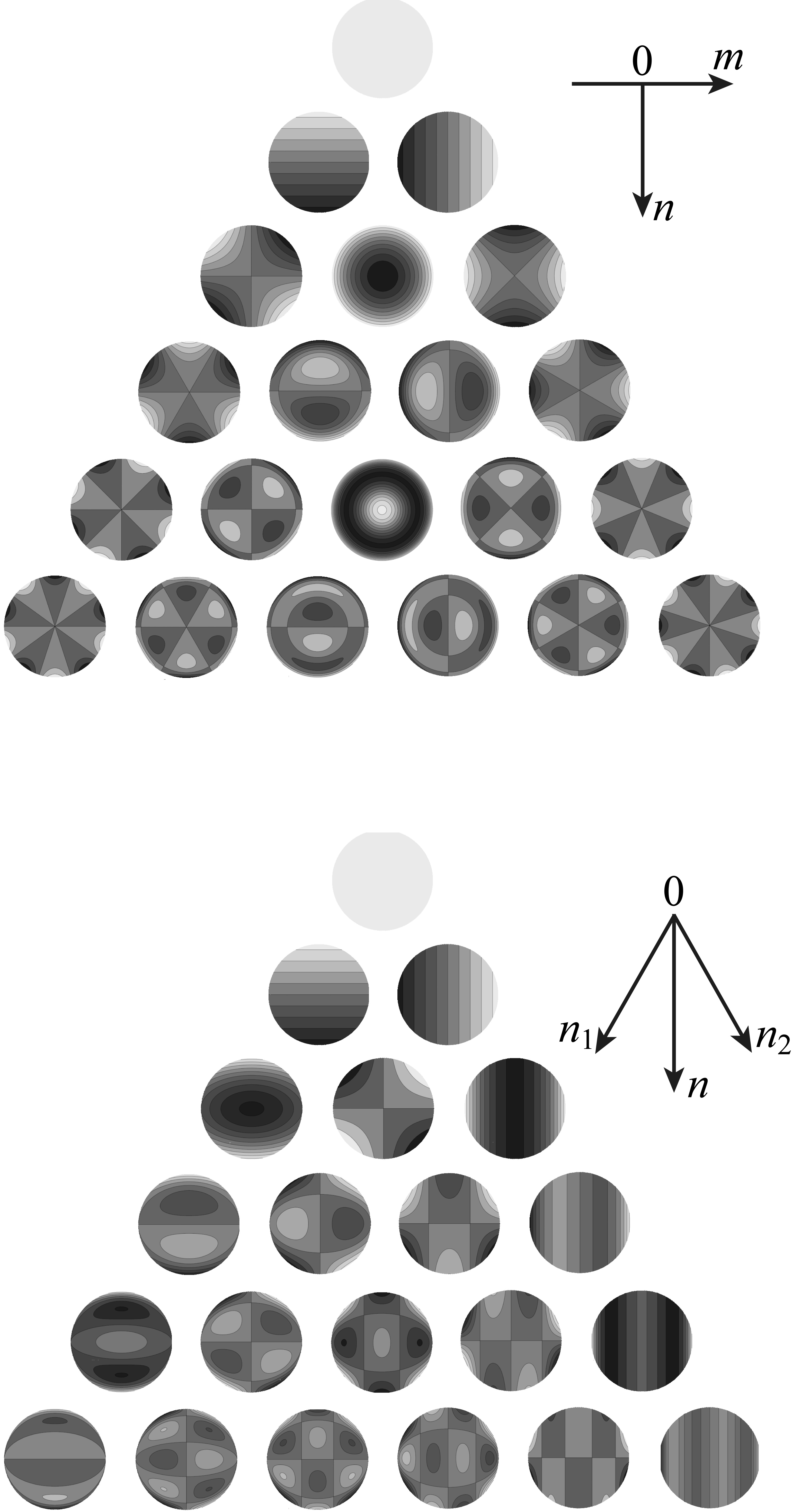
Figure 2: Top: The basis of Zernike solutions $\Psi^{\scriptscriptstyle\rm I}_{n,m}(r,\phi)$ in (12), normalized on the disk and classified by principal and angular momentum quantum numbers $(n,m)$. Since they are complex, we show Re$\,\Psi^{\scriptscriptstyle\rm I}_{n,m}$ for $m\geq 0$ and Im$\,\Psi^{\scriptscriptstyle\rm I}_{n,m}$ for $m<0$. Bottom: The new real solutions $\Psi^{\scriptscriptstyle\rm II}_{n,m}(r,\phi)$ in (17) of Zernike’s equation (1) in the coordinate system II, classified by the quantum numbers $(n_{1},n_{2})$ (as if they were two-dimensional quantum harmonic oscillator states —which they are not). Figure by Cristina Salto-Alegre.

2.3 Solutions in System II (9)

The Zernike differential equation in the form (6), after replacement of the second coordinate system $(\vartheta^{\prime},\varphi^{\prime})$ in (9) on the half-sphere, acting on functions separated as

$$\Upsilon^{\scriptscriptstyle\rm II}(\vartheta^{\prime},\varphi^{\prime})=\frac{1}{\sqrt{\sin\vartheta^{\prime}}}S(\vartheta^{\prime})\,T(\varphi^{\prime}),$$ (13)

yields a system of two simultaneous differential equations bound by a separation constant $k$, whose Pöschl-Teller form is most evident in variables $\mu={\textstyle\frac{1}{2}}\varphi^{\prime}$ and $\nu={\textstyle\frac{1}{2}}\vartheta^{\prime}$,

$$\frac{{\rm d}^{2}T(\mu)}{{\rm d}\mu^{2}}+\bigg{(}4k^{2}+\frac{1}{4\sin^{2}\mu}+\frac{1}{4\cos^{2}\mu}\bigg{)}T(\mu) = 0,$$ (14)

$$\frac{{\rm d}^{2}S(\nu)}{{\rm d}\nu^{2}}+\bigg{(}(E+1)^{2}+\frac{1-4k^{2}}{4\sin^{2}\nu}+\frac{1-4k^{2}}{4\cos^{2}\mu}\bigg{)}S(\nu) = 0.$$ (15)

Finally, as shown in [8] and determined by the boundary conditions, two quantum numbers $n_{1},n_{2}\in{\cal Z}_{0}^{+}$ are imposed for the solutions on ${\cal H}_{+}$, yielding Gegenbauer polynomials in $\cos\vartheta^{\prime}$ and Legendre polynomials in $\cos\varphi^{\prime}$. These are

$$\Upsilon^{\scriptscriptstyle\rm II}_{n_{1},n_{2}}(\vartheta^{\prime},\varphi^{\prime}) := C_{n_{1},n_{2}}\,(\sin\vartheta^{\prime})^{n_{1}+1/2}(\sin\varphi^{\prime})^{1/2}\,C_{n_{2}}^{n_{1}+1}(\cos\vartheta^{\prime})\,P_{n_{1}}(\cos\varphi^{\prime}),$$

$$C_{n_{1},n_{2}} := 2^{n_{1}}n_{1}!\sqrt{\frac{(2n_{1}+1)(n_{1}+n_{2}+1)\,n_{2}!}{\pi\,(2n_{1}+n_{2}+1)!}},$$ (16)

where the principal quantum number is $n=n_{1}+n_{2}\in{\cal Z}_{0}^{+}$, and with the $E=n(n{+}2)$ as before. The orthonormality of these solutions is also over the half-sphere ${\cal H}_{+}$ under the formally same measure ${\rm d}^{2}S^{\scriptscriptstyle\rm II}(\vartheta^{\prime},\varphi^{\prime})=\sin\vartheta^{\prime}\,{\rm d}\vartheta^{\prime}\,{\rm d}\varphi^{\prime}$ where the angles have the range (9).

On the disk in Cartesian coordinates ${\bf r}=(x,y)$, the solutions are

$$\Psi^{\scriptscriptstyle\rm II}_{n_{1},n_{2}}(x,y)=C_{n_{1},n_{2}}\,(1-x^{2})^{n_{1}/2}\,C^{n_{1}+1}_{n_{2}}(x)\,P_{n_{1}}\bigg{(}\frac{y}{\sqrt{1-x^{2}}}\bigg{)},$$ (17)

separated in the non-orthogonal coordinates $x$ and $y/\surd(1-x^{2})$, and normalized under the inner product on $\cal D$ in (5). These are shown in Fig. 2 (bottom).

3 Expansion between I and II solutions

The two bases of solutions of the Zernike equation in the coordinate systems I and II on the half-sphere, $\Upsilon^{\scriptscriptstyle\rm I}_{n,m}(\vartheta,\varphi)$ in (11) and $\Upsilon^{\scriptscriptstyle\rm II}_{n_{1},n_{2}}(\vartheta^{\prime},\varphi^{\prime})$ in (16), with the same principal quantum number $n$,

$$\begin{array}[]{c}n_{1}+n_{2}=n=2n_{r}+{{\scriptstyle|}m{\scriptstyle|}}\in{\cal Z}_{0}^{+},\\ n_{r},n_{1},n_{2}\in{\cal Z}_{0}^{+},\quad m\in\{-n,-n{+}2,\ldots,n\},\end{array}$$ (18)

whose projections on the disk are shown in Fig. 2, were arranged into pyramids with rungs labelled by $n$, and containing $n+1$ states each. They could be mistakenly seen as independent su($2$) multiplets of spin $j={\textstyle\frac{1}{2}}n$ because, as we said above, in system II they are not bases for this Lie algebra. Nevertheless, in each rung $n$, the two bases must relate through linear combination

$$\Upsilon^{\scriptscriptstyle\rm II}_{n_{1},n_{2}}(\vartheta^{\prime},\varphi^{\prime})=\!\!\!\sum_{m=-n\,\scriptscriptstyle(2)}^{n}\!\!\!W_{n_{1},n_{2}}^{n,m}\,\Upsilon^{\scriptscriptstyle\rm I}_{n,m}(\vartheta,\varphi),$$ (19)

where $\sum_{m=-n\,\scriptscriptstyle(2)}^{n}$ indicates that $m$ takes values separated by 2 as in (18). The relation between the primed and unprimed angles in (8) and (9) is

$$\begin{array}[]{rl}{}\quad\cos\vartheta^{\prime}=\sin\vartheta\cos\varphi,&\sin\vartheta^{\prime}=\sqrt{1-\sin^{2}\vartheta\cos^{2}\varphi},\\[3.0pt] \displaystyle\cos\varphi^{\prime}=\frac{\sin\vartheta\sin\varphi}{\sqrt{1-\sin^{2}\vartheta\cos^{2}\varphi}},&\displaystyle\sin\varphi^{\prime}=\frac{\cos\vartheta}{\sqrt{1-\sin^{2}\vartheta\cos^{2}\varphi}}.\end{array}$$ (20)

To find the linear combination coefficients $W_{n_{1},n_{2}}^{n,m}$ in (19), we compute first the relation (19) near to the boundary of the disk and sphere, at $\vartheta={\textstyle\frac{1}{2}}\pi-\varepsilon$ for small $\varepsilon$, so that $\cos\vartheta=-\sin\varepsilon\approx-\varepsilon$ and $\sin\vartheta=\cos\varepsilon\approx 1-{\textstyle\frac{1}{2}}\varepsilon^{2}$. There, (20) becomes

$$\begin{array}[]{rl}{}\quad\cos\vartheta^{\prime}\approx\cos\varphi,&\sin\vartheta^{\prime}\approx\sin\varphi,\\[3.0pt] \displaystyle\cos\varphi^{\prime}\approx\cos\varepsilon,&\displaystyle\sin\varphi^{\prime}\approx-\sin\varepsilon/\sin\varphi.\end{array}$$ (21)

Hence, when $\varepsilon\to 0$ is at the rim of the disk and sphere, after dividing (19) by $\surd(-\varepsilon)$ on both sides, this relation reads

$$C_{n_{1},n_{2}}\,(\sin\varphi)^{n_{1}}C^{n_{1}+1}_{n_{2}}(\cos\varphi)\,P_{n}(1)=\sqrt{\frac{n{+}1}{\pi}}\!\!\!\sum_{m=-n\,\scriptscriptstyle(2)}^{n}\!\!\!W_{n_{1},n_{2}}^{n,m}\,P^{({{\scriptscriptstyle|}m{\scriptscriptstyle|}},0)}_{n_{r}}(-1)\,e^{{\rm i}m\varphi},$$ (22)

with $n_{r}=\frac{1}{2}(n-{{\scriptscriptstyle|}m{\scriptscriptstyle|}})$. Recalling that $P_{n_{1}}(1)=1$ and $P^{({{\scriptscriptstyle|}m{\scriptscriptstyle|}},0)}_{n_{r}}(-1)=(-1)^{n_{r}}$, we can now use the orthogonality of the $e^{{\rm i}m\varphi}$ functions to express the interbasis coefficients as a Fourier integral,

$$W_{n_{1},n_{2}}^{n,m}=\frac{(-1)^{n_{r}}\,C_{n_{1},n_{2}}}{2\sqrt{\pi(n{+}1)}}\int_{-\pi}^{\pi}{\rm d}\varphi\,(\sin\varphi)^{n_{1}}C^{n_{1}+1}_{n_{2}}(\cos\varphi)\,\exp(-{\rm i}m\varphi).$$ (23)

The integral (23) does not appear as such in the standard tables [12]; in Appendix A we derive the result and show that it can be written in terms of a hypergeometric ${}_{3}F_{2}$ polynomial which are su($2$) Clebsch-Gordan coefficients of a special structure,

$$W^{n,m}_{n_{1},n_{2}}=\frac{{\rm i}^{n_{1}}(-1)^{(m+|m|)/{2}}\,n_{1}!\,(n_{1}+n_{2})!}{\Big{(}{\textstyle\frac{1}{2}}(n_{1}{+}n_{2}{+}m)\Big{)}!\,\Big{(}{\textstyle\frac{1}{2}}({n_{1}{-}n_{2}{-}m})\Big{)}!}\,\sqrt{\frac{2n_{1}+1}{n_{2}!\,(2n_{1}+n_{2}+1)!}}$$

$${\qquad\qquad\qquad}\times{{}_{3}F_{2}}\left({-n_{2},\quad n_{1}+1,\quad-{\textstyle\frac{1}{2}}(n_{1}+n_{2}+m)\atop-n_{1}-n_{2},\quad{\textstyle\frac{1}{2}}(n_{1}-n_{2}-m)+1}\Bigg{|}\,\,1\right)$$ (24)

$$\phantom{W^{n,m}_{n_{1},n_{2}}\,}={\rm i}^{n_{1}}(-1)^{(m+|m|)/{2}}\,C^{n_{1},\ 0}_{\frac{1}{2}n,\,-\frac{1}{2}m;\ \frac{1}{2}n,\,\frac{1}{2}m},$$ (25)

where we have used the notation of Varshalovich et al. in Ref. [13] that couples the su($2$) states $(j_{1},m_{1})$ and $(j_{2},m_{2})$ to $(j,m)$, as $C^{j,m}_{j_{1},m_{1};\,j_{2},m_{2}}\equiv C{\textstyle{j_{1},\atop m_{1},}{j_{2},\atop m_{2},}{j\atop m}}\equiv\langle j_{1},m_{1};\,j_{2},m_{2}|(j_{1},j_{2})\,j,m\rangle.$

One can then use the orthonormality properties of the Clebsch-Gordan coefficients to write the transformation inverse to (19) as

$$\Upsilon^{\scriptscriptstyle\rm I}_{n,m}(\vartheta,\varphi) = \sum_{n_{1}=0}^{n}\widetilde{W}^{n_{1},n_{2}}_{n,m}\,\Upsilon^{\scriptscriptstyle\rm II}_{n_{1},n_{2}}(\vartheta^{\prime},\varphi^{\prime}),$$ (26)

$$\widetilde{W}_{n,m}^{n_{1},n_{2}} = (-{\rm i})^{n_{1}}(-1)^{(m+|m|)/{2}}\,C^{n_{1},\ 0}_{\frac{1}{2}n,\,-\frac{1}{2}m;\ \frac{1}{2}n,\,\frac{1}{2}m},$$ (27)

with $n_{1}+n_{2}=n$. The relation between the unprimed and primed angles of the coordinate systems I and II is the inverse of (20), namely

$$\begin{array}[]{rl}{}\quad\cos\vartheta=\sin\vartheta^{\prime}\sin\varphi^{\prime},&\sin\vartheta=\sqrt{1-\sin^{2}\vartheta^{\prime}\sin^{2}\varphi^{\prime}},\\[3.0pt] \displaystyle\cos\varphi=\frac{\cos\vartheta^{\prime}}{\sqrt{1-\sin^{2}\vartheta^{\prime}\sin^{2}\varphi^{\prime}}},&\displaystyle\sin\varphi=\frac{\sin\vartheta^{\prime}}{\sqrt{1-\sin^{2}\vartheta^{\prime}\sin^{2}\varphi^{\prime}}}.\end{array}$$ (28)

4 Concluding remarks

The new polynomial solutions of the Zernike differential equation (1) can be of further use in the treatment of generally off-axis wavefront aberrations in circular pupils. While the original basis of Zernike polynomials $\Psi^{\scriptscriptstyle\rm I}_{n,m}(r,\phi)$ serves naturally for axis-centered aberrations, the new basis $\Psi^{\scriptscriptstyle\rm II}_{n_{1},n_{2}}(r,\phi)$ in (17) includes, for $n_{1}=0$, plane wave-trains with $n_{2}$ nodes along the $x$-axis of the pupil, which are proportional to $U_{n_{2}}(x)$, the Chebyshev polynomials of the second kind.

We find that the Zernike system is also very relevant for studies of ‘non-standard’ symmetries described by Higgs algebras. While rotations in the basis of spherical harmonics is determined through the Wigner-$D$ functions [13] of the rotation angles on the sphere, here the boundary conditions of the disk and sphere allow for only a ${\textstyle\frac{1}{2}}\pi$-rotation of the $z$-axis to orientations in $x$–$y$ plane, and the basis functions do not relate through Wigner $D$-functions, but Clebsch-Gordan coefficients of a special type. Since the classical and quantum Zernike systems analysed in [8, 9] have several new and exceptional properties, we surmise that applications not yet evident in this paper must also be of interest.

Appendix A. The integral (23) and Clebsch-Gordan coefficients

The integral in (23) does not seem to be in the literature, although similar integrals appear in a paper of Kildyushov [14] to calculate his three coefficients. Thus let us solve ab initio, with $\lambda=n_{1}$ and $\nu=n_{2}$, integrals of the kind

$$I_{\nu}^{\lambda,m}:=\int_{-\pi}^{\pi}{\rm d}\varphi\,\sin^{\lambda}\!\varphi\,\,C_{\nu}^{\lambda+1}(\cos\varphi)\,e^{-{\rm i}m\varphi},\quad\lambda,\nu\in\{0,1,2,\ldots\}.$$ (29)

We write the trigonometric function and the Gegenbauer polynomial in their Fourier series expansions,

$$\sin^{\lambda}\varphi = \frac{e^{{\rm i}\lambda\varphi}}{(2{\rm i})^{\lambda}}(1-e^{-2{\rm i}\varphi})^{\lambda}=\frac{1}{(2{\rm i})^{\lambda}}\sum\limits_{k=0}^{\lambda}\frac{(-1)^{k}\,\lambda!}{k!\,(\lambda-k)!}\,e^{{\rm i}(\lambda-2k)\varphi},$$ (30)

$$C^{\lambda+1}_{\nu}(\cos\varphi) = \sum\limits_{l=0}^{\nu}\frac{(\lambda+l)!}{l!\,(\nu-l)!}\frac{(\lambda+\nu-l)!}{(\lambda!)^{2}}e^{-{\rm i}(\nu-2l)\varphi}.$$ (31)

Substituting these expansions in (29), using the orthogonality of the $e^{{\rm i}\kappa\varphi}$ functions and thereby eliminating one of the two sums, we find a ${}_{3}F_{2}$ hypergeometric series for unit argument,

$$I_{\nu}^{\lambda,m}=\frac{2\pi}{(2{\rm i})^{\lambda}}\frac{(\lambda{+}\nu)!}{\nu!}\frac{(-1)^{(\lambda-\nu-m)/2}}{\Big{(}{\textstyle\frac{1}{2}}(\lambda-\nu-m)\Big{)}!\,\Big{(}{\textstyle\frac{1}{2}}(\lambda+\nu+m)\Big{)}!}$$

$${\qquad\qquad}\times{{}_{3}F_{2}}\left({-\nu,\quad\lambda+1,\quad-{\textstyle\frac{1}{2}}(\lambda+\nu+m)\atop-\lambda-\nu,\quad{\textstyle\frac{1}{2}}(\lambda-\nu-m)+1}\Bigg{|}\,\,1\right).$$ (32)

Multiplying this by the coefficients $C_{n_{1},n_{2}}$ in (23), one finds the first expression in (24).

In order to relate the previous result with the su($2$) Clebsch-Gordan coefficients in (25), we use the formula in [13, Eq. (21), Sect. 8.2] for the particular case at hand, and a relation between ${}_{3}F_{2}$-hypergeometric functions,

$${{}_{3}F_{2}}\left({a,\ b,\ c\atop d,\ e}\Bigg{|}\,\,1\right)=\frac{\Gamma(d)\,\Gamma(d{-}a{-}b)}{\Gamma(d{-}a)\,\Gamma(d{-}b)}\,\,{{}_{3}F_{2}}\left({a,\ b,\ e{-}c\atop a{+}b{-}d{+}1,\ e}\Bigg{|}\,\,1\right),$$ (33)

to write these particularly symmetric coefficients as

$$C^{\gamma,0}_{\alpha,\,-\beta;\ \alpha,\,\beta}=\frac{(2\alpha)!\,\gamma!}{(\alpha+\beta)!\,(\gamma-\alpha-\beta)!}\sqrt{\frac{2\gamma+1}{(2\alpha-\gamma)!\,(2\alpha+\gamma+1)!}}$$

$${\qquad\qquad\qquad}\times{{}_{3}F_{2}}\left({-2\alpha+\gamma,\quad\gamma+1,\quad-\alpha-\beta\atop-2\alpha,\quad\gamma-\alpha-\beta+1}\Bigg{|}\,\,1\right).$$ (34)

Finally, upon replacement of $\gamma=n_{1}$, $\alpha={\textstyle\frac{1}{2}}n={\textstyle\frac{1}{2}}(n_{1}+n_{2})$ and $\beta={\textstyle\frac{1}{2}}m$, the expression (24) reduces to (25) times the phase and sign.

Appendix B. The lowest $W^{n,m}_{n_{1},n_{2}}$ coefficients

The interbasis expansion coefficients binding the two bases in (19) and Fig. 2, can be seen as $(n+1)\times(n+1)$ matrices ${\bf W}_{\!\!{{\scriptscriptstyle(}n{\scriptscriptstyle)}}}=\|W^{n,m}_{n_{1},n_{2}}\|$ with composite rows $(n_{1},n_{2})$ and columns $(n,m)$ for each rung $n_{1}+n_{2}=n\in{\cal Z}_{0}^{+}$, on $(n+1)$-dimensional column vectors of functions as ${\bf\Upsilon}^{\scriptscriptstyle\rm II}(\vartheta^{\prime},\varphi^{\prime})={\bf W}_{\!\!{{\scriptscriptstyle(}n{\scriptscriptstyle)}}}{\bf\Upsilon}^{\scriptscriptstyle\rm I}(\vartheta,\varphi)$. The elements $W^{n,m}_{n_{1},n_{2}}$ in (25) are the product of phases

$${\rm i}^{n_{1}},\qquad(-1)^{\pm\frac{1}{2}(m+{{\scriptscriptstyle|}m{\scriptscriptstyle|}})}=\left\{\begin{array}[]{ll}(-1)^{m},&m>0,\\ 1,&m\leq 0,\end{array}\right.$$ (35)

times the special Clebsch-Gordan coefficients $C^{n_{1},0}_{\frac{1}{2}n,-\frac{1}{2}m;\frac{1}{2}n,\frac{1}{2}m}$

For the first five rungs in Fig. 2, these are

For $n=0$: $W_{\!\!(0)}=C^{0,0}_{0,0;0,0}=1$,

$${\hskip-15.0pt}{\bf W}_{\!\!(1)}=\bordermatrix{&m=1&-1\cr n_{1}{=}1&-{\rm i}C^{1,0}_{\frac{1}{2},-\frac{1}{2};\frac{1}{2},\frac{1}{2}}&{\rm i}C^{1,0}_{\frac{1}{2},\frac{1}{2};\frac{1}{2},-\frac{1}{2}}\cr{}\hfill 0&-C^{0,0}_{\frac{1}{2},-\frac{1}{2};\frac{1}{2},\frac{1}{2}}&C^{0,0}_{\frac{1}{2},\frac{1}{2};\frac{1}{2},-\frac{1}{2}}\cr},$$

$${\hskip-20.0pt}{\bf W}_{\!\!(2)}=\bordermatrix{&m=2&0&-2\cr n_{1}{=}2&-C^{2,0}_{1,-1;1,1}&-C^{2,0}_{1,0;1,0}&-C^{2,0}_{1,1;1,-1}\cr{}\hfill 1&{\rm i}C^{1,0}_{1,-1;1,1}&0&{\rm i}C^{1,0}_{1,1;1,-1}\cr{}\hfill 0&C^{0,0}_{1,-1;1,1}&C^{0,0}_{1,0;1,0}&C^{0,0}_{1,1;1,-1}\cr},$$

$${\hskip-20.0pt}{\bf W}_{\!\!(3)}={}\hskip-14.22636pt\bordermatrix{&m=3&1&-1&-3\cr n_{1}{=}3&{\rm i}C^{3,0}_{\frac{3}{2},-\frac{3}{2};\frac{3}{2},\frac{3}{2}}&{\rm i}C^{3,0}_{\frac{3}{2},-\frac{1}{2};\frac{3}{2},\frac{1}{2}}&-{\rm i}C^{3,0}_{\frac{3}{2},\frac{1}{2};\frac{3}{2},-\frac{1}{2}}&-{\rm i}C^{3,0}_{\frac{3}{2},\frac{3}{2};\frac{3}{2},-\frac{3}{2}}\cr{}\hfill 2&C^{2,0}_{\frac{3}{2},-\frac{3}{2};\frac{3}{2},\frac{3}{2}}&C^{2,0}_{\frac{3}{2},-\frac{1}{2};\frac{3}{2},\frac{1}{2}}&-C^{2,0}_{\frac{3}{2},\frac{1}{2};\frac{3}{2},-\frac{1}{2}}&-C^{2,0}_{\frac{3}{2},\frac{3}{2};\frac{3}{2},-\frac{3}{2}}\cr{}\hfill 1&-{\rm i}C^{1,0}_{\frac{3}{2},-\frac{3}{2};\frac{3}{2},\frac{3}{2}}&-{\rm i}C^{1,0}_{\frac{3}{2},-\frac{1}{2};\frac{3}{2},\frac{1}{2}}&{\rm i}C^{1,0}_{\frac{3}{2},\frac{1}{2};\frac{3}{2},-\frac{1}{2}}&{\rm i}C^{1,0}_{\frac{3}{2},\frac{3}{2};\frac{3}{2},-\frac{3}{2}}\cr{}\hfill 0&-C^{0,0}_{\frac{3}{2},-\frac{3}{2};\frac{3}{2},\frac{3}{2}}&-C^{0,0}_{\frac{3}{2},-\frac{1}{2};\frac{3}{2},\frac{1}{2}}&C^{0,0}_{\frac{3}{2},\frac{1}{2};\frac{3}{2},-\frac{1}{2}}&C^{0,0}_{\frac{3}{2},\frac{3}{2};\frac{3}{2},-\frac{3}{2}}\cr},$$

$${\hskip-20.0pt}{\bf W}_{\!\!(4)}={}\hskip-14.22636pt\bordermatrix{&m=4&2&0&-2&-4\cr n_{1}{=}4&C^{4,0}_{2,-2;2,2}&C^{4,0}_{2,-1;2,1}&C^{4,0}_{2,0;2,0}&C^{4,0}_{2,1;2,-1}&C^{4,0}_{2,2;2,-2}\cr{}\hfill 3&-{\rm i}C^{3,0}_{2,-2;2,2}&-{\rm i}C^{3,0}_{2,-1;2,1}&0&-{\rm i}C^{3,0}_{2,1;2,-1}&-{\rm i}C^{3,0}_{2,2;2,-2}\cr{}\hfill 2&-C^{2,0}_{2,-2;2,2}&-C^{2,0}_{2,-1;2,1}&-C^{2,0}_{2,0;2,0}&-C^{2,0}_{2,1;2,-1}&-C^{2,0}_{2,2;2,-2}\cr{}\hfill 1&{\rm i}C^{1,0}_{2,-2;2,2}&{\rm i}C^{1,0}_{2,-1;2,1}&0&{\rm i}C^{1,0}_{2,1;2,-1}&{\rm i}C^{1,0}_{2,2;2,-2}\cr{}\hfill 0&C^{0,0}_{2,-2;2,2}&C^{0,0}_{2,-1;2,1}&C^{0,0}_{2,0;2,0}&C^{0,0}_{2,1;2,-1}&C^{0,0}_{2,2;2,-2}\cr},$$

where some elements are zero because $C^{n_{1},0}_{\frac{1}{2}n,0;\,\frac{1}{2}n,0}=0$ for even $n$ and odd $n_{1}$.

The Zernike polynomials come in complex conjugate pairs, $\Upsilon^{\scriptscriptstyle\rm I}_{n,m}=\Upsilon^{\scriptscriptstyle\rm I\,*}_{n,-m}$, while the $\Upsilon^{\scriptscriptstyle\rm II}_{n_{1},n_{2}}$’s are real. The linear combinations afforded by the ${\bf W}$ matrices above indeed yield real functions because

$$C^{n_{1},0}_{\frac{1}{2}n,-\frac{1}{2}m;\,\frac{1}{2}n,\frac{1}{2}m}=(-1)^{n_{2}}C^{n_{1},0}_{\frac{1}{2}n,\frac{1}{2}m;\,\frac{1}{2}n,-\frac{1}{2}m}.$$ (36)

References

- [1] F. Zernike, Beugungstheorie des Schneidenverfahrens und Seiner Verbesserten Form der Phasenkontrastmethode, Physica 1, 689–704 (1934).
- [2] A. B. Bhatia and E. Wolf, On the circle polynomials of Zernike and related orthogonal sets, Math. Proc. Cambridge Phil. Soc. 50, 40–48 (1954).
- [3] T. H. Koornwinder, Two-variable analogues of the classical orthogonal polynomials. In: R. A. Askey (Ed.), Theory and Application of Special Functions (Academic Press, New York, 1975), pp. 435-–495.
- [4] E. C. Kintner, On the mathematical properties of the Zernike Polynomials, Opt. Acta 23, 679–680 (1976).
- [5] A. Wünsche, Generalized Zernike or disc polynomials, J. Comp. App. Math. 174, 135–163 (2005).
- [6] B. H. Shakibaei and R. Paramesran, Recursive formula to compute Zernike radial polynomials, Opt. Lett. 38, 2487–2489 (2013).
- [7] M. E. H. Ismail and R. Zhang, Classes of bivariate orthogonal polynomials, arXiv:1502.07256v3 [math.CA].
- [8] G. S. Pogosyan, K. B. Wolf, and A. Yakhno, Superintegrable classical Zernike system, J. Math. Phys. submitted, (2017).
- [9] G. S. Pogosyan, C. Salto-Alegre, K. B. Wolf, and A. Yakhno, Superintegrable quantum Zernike system, J. Math. Phys. submitted, (2017).
- [10] P. W. Higgs, Dynamical symmetries in a spherical geometry, J. Phys. A 12, 309–323 (1979).
- [11] G. S. Pogosyan, A. N. Sissakian and P. Winternitz, Separation of variables and Lie algebra contractions. Applications to special functions, Phys. Part. Nuclei 33, Suppl. 1, S123–S144 (2002).
- [12] I. S. Gradshteyn and I. M. Ryzhik, Table of Integrals, Series and Products, 7th ed. (Elsevier, 2007),
- [13] D. A. Varshalovich, A. N. Moskalev, and V. K. Khersonskiĭ, Quantum Theory of Angular Momentum (World Scientific, Singapore, 1988).
- [14] M. S. Kildyushov, Hyperspherical functions of “three” type in the -Body Problem, J. Nucl. Phys. (Yadernaya Fizika) 15, 187–208 (1972) (in Russian).