Parallel Matrix-Free Implementation of Frequency-Domain        Finite Difference Methods for Cluster Computing

Abstract

Full-wave 3D electromagnetic simulations of complex planar devices, multilayer interconnects, and chip packages are presented for wide-band frequency-domain analysis using the finite difference integration technique developed in the PETSc software package. Initial reordering of the index assignment to the unknowns makes the resulting system matrix diagonally dominant. The rearrangement also facilitates the decomposition of large domain into slices for passing the mesh information to different machines. Matrix-free methods are then exploited to minimize the number of element-wise multiplications and memory requirements in the construction of the system of linear equations. Besides, the recipes provide extreme ease of modifications in the kernel of the code. The applicability of different Krylov subspace solvers is investigated. The accuracy is checked through comparisons with CST MICROWAVE STUDIO^® transient solver results. The parallel execution of the compiled code on specific number of processors in multi-core distributed-memory architectures demonstrate high scalability of the computational algorithm.

1 Introduction

The integrated circuits (IC) industry has previously practiced the extraction of equivalent lumped-element models as a simulation tool for hardware design. Advances in semiconductor interconnect technology, such as ever increasing clock frequency and package density, however, demand full-wave analysis of a product-level model to preserve the signal integrity in high-speed electronic devices [1], [2]. As a general multi-grid difference-based electromagnetic field solver tool [3], [4], the finite integration technique (FIT) provides a direct discretization of the Maxwell’s equations in their integral form using voltages and fluxes, respectively, along the edges and surfaces of a pair of interlaced structured grids [5], [6].

To perform matrix-vector products for the matrices that do not fit in the cache, CPU requires more time to calling the matrix entries from the main memory than performing the floating-point multiplications and additions. Matrix-free methods, instead of saving the matrix in memory, recompute the operator representing matrix elements with additional floating-point operations [7]. On the other hand, the matrix-free methods are not able to use black-box preconditioners.

Modern object-oriented programming paradigms supply an enormous level of abstraction in mechanisms needed within parallel computing [8]. The software package PETSc (Portable, Extensible Toolkit for Scientific Computation) consists of an expanding set of data structures and routines such as parallel matrix and vector assembly which provide building blocks for facilitating the development of scientific application codes on parallel (and serial) computers [9]. PETSc uses the MPI standard for message-passing communications and it provides a collection of Krylov subspace (KSP) methods which can be employed as parallel linear solvers for the frequency-domain FIT matrix systems. This paper works out how the PETSc shell matrix concept can create a foundation for building and solving large-scale FIT systems on parallel processors. It is shown that the computational speed and memory demands of 3D finite-difference frequency-domain (FDFD)-based electromagnetic solvers can be scaled down simultaneously using the advanced parallel programming tools.

The remainder of this report is organized as follows. In Section II, the FIT discretization scheme is briefly explained. Section III includes implementation aspects of the matrix-free-based electromagnetic-field solver. In Section IV, the accuracy of the developed code is checked through eigenmode calculations in a rectangular cavity as well as comparisons with CST MICROWAVE STUDIO^® (MWS) discrete-port results [10]. The overall performance of the parallelized algorithm is measured on cluster of computers. Numerical simulations of complex planar devices, multilayer interconnects, and chip packages are presented.

2 Finite Integration Technique

The FIT renders a consistent transformation of the integral form of Maxwell’s equations into a set of matrix equations with a unique solution [5]. Maxwell’s equations are hereby discretized on a pair of spatially staggered grids, namely the primal and dual grid $(G,\widetilde{G})$ with edge lengths $(L_{n},\widetilde{L}_{n})$ and facet surface areas $(A_{n},\widetilde{A}_{n})$, respectively, where the dual cell gridpoints $\widetilde{G}$ are defined on the barycenter of the primary cell mesh $G$ [11]. The state variables of the FIT are the electric and magnetic grid voltages

$${\begin{picture}(9.0,12.5)\put(0.0,0.0){\makebox(9.0,12.0)[b]{$\stackrel{{\scriptstyle\begin{picture}(4.0,1.0)\put(0.0,-2.0){$\scriptscriptstyle\smallfrown$} \end{picture}}}{{\rule[0.0pt]{1.0pt}{0.0pt}e}}$}} \end{picture}}_{n}=\int_{L_{n}}{\bf E}({\bf r},t)\cdot{\rm d}{\bf l},\quad{\begin{picture}(9.0,12.5)\put(0.0,0.0){\makebox(9.0,12.0)[b]{$\stackrel{{\scriptstyle\begin{picture}(4.0,1.0)\put(0.0,-2.0){$\scriptscriptstyle\smallfrown$} \end{picture}}}{{\rule[0.0pt]{1.0pt}{0.0pt}h}}$}} \end{picture}}_{n}=\int_{\widetilde{L}_{n}}{\bf H}({\bf r},t)\cdot{\rm d}{\bf l},$$

the electric and magnetic grid fluxes

$${\begin{picture}(9.0,12.5)\put(0.0,0.0){\makebox(9.0,12.0)[b]{$\stackrel{{\scriptstyle\begin{picture}(4.0,3.0)\put(0.0,-2.0){$\scriptscriptstyle\smallfrown$} \put(0.0,-0.5){$\scriptscriptstyle\smallfrown$} \end{picture}}}{{\rule[0.0pt]{1.0pt}{0.0pt}d}}$}} \end{picture}}_{n}=\int_{\widetilde{A}_{n}}{\bf D}({\bf r},t)\cdot{\rm d}{\bf A},\quad{\begin{picture}(9.0,12.5)\put(0.0,0.0){\makebox(9.0,12.0)[b]{$\stackrel{{\scriptstyle\begin{picture}(4.0,3.0)\put(0.0,-2.0){$\scriptscriptstyle\smallfrown$} \put(0.0,-0.5){$\scriptscriptstyle\smallfrown$} \end{picture}}}{{\rule[0.0pt]{1.0pt}{0.0pt}b}}$}} \end{picture}}_{n}=\int_{A_{n}}{\bf B}({\bf r},t)\cdot{\rm d}{\bf A},$$

passing through surfaces of the pair of interlaced structured grids, as well as the current

$${\begin{picture}(9.0,12.5)\put(0.0,0.0){\makebox(9.0,12.0)[b]{$\stackrel{{\scriptstyle\begin{picture}(4.0,3.0)\put(0.0,-2.0){$\scriptscriptstyle\smallfrown$} \put(0.0,-0.5){$\scriptscriptstyle\smallfrown$} \end{picture}}}{{\rule[0.0pt]{1.0pt}{0.0pt}j}}$}} \end{picture}}_{n}=\int_{\widetilde{A}_{n}}{\bf J}({\bf r},t)\cdot{\rm d}{\bf A}.$$

Storing the discrete components in vectors , , , , and , the Faraday’s and Ampère’s laws can be transformed into a set of grid equations

$${\bf C}{\begin{picture}(9.0,12.5)\put(0.0,0.0){\makebox(9.0,12.0)[b]{$\stackrel{{\scriptstyle\begin{picture}(4.0,1.0)\put(0.0,-2.0){$\scriptscriptstyle\smallfrown$} \end{picture}}}{{\rule[0.0pt]{1.0pt}{0.0pt}\bf e}}$}} \end{picture}}=-\frac{\rm d}{{\rm d}t}{\begin{picture}(9.0,12.5)\put(0.0,0.0){\makebox(9.0,12.0)[b]{$\stackrel{{\scriptstyle\begin{picture}(4.0,3.0)\put(0.0,-2.0){$\scriptscriptstyle\smallfrown$} \put(0.0,-0.5){$\scriptscriptstyle\smallfrown$} \end{picture}}}{{\rule[0.0pt]{1.0pt}{0.0pt}\bf b}}$}} \end{picture}}, \quad\widetilde{\bf C}{\begin{picture}(9.0,12.5)\put(0.0,0.0){\makebox(9.0,12.0)[b]{$\stackrel{{\scriptstyle\begin{picture}(4.0,1.0)\put(0.0,-2.0){$\scriptscriptstyle\smallfrown$} \end{picture}}}{{\rule[0.0pt]{1.0pt}{0.0pt}\bf h}}$}} \end{picture}}=\frac{\rm d}{{\rm d}t}{\begin{picture}(9.0,12.5)\put(0.0,0.0){\makebox(9.0,12.0)[b]{$\stackrel{{\scriptstyle\begin{picture}(4.0,3.0)\put(0.0,-2.0){$\scriptscriptstyle\smallfrown$} \put(0.0,-0.5){$\scriptscriptstyle\smallfrown$} \end{picture}}}{{\rule[0.0pt]{1.0pt}{0.0pt}\bf d}}$}} \end{picture}}+{\begin{picture}(9.0,12.5)\put(0.0,0.0){\makebox(9.0,12.0)[b]{$\stackrel{{\scriptstyle\begin{picture}(4.0,3.0)\put(0.0,-2.0){$\scriptscriptstyle\smallfrown$} \put(0.0,-0.5){$\scriptscriptstyle\smallfrown$} \end{picture}}}{{\rule[0.0pt]{1.0pt}{0.0pt}\bf j}}$}} \end{picture}}$$ (1)

in which the matrices ${\bf C}$ and $\widetilde{\bf C}$ are, respectively, the discrete curl-operators on the primal and dual grid. Owing to the topological nature, $\widetilde{\bf C}={\bf C}^{\rm T}$ where ${\rm T}$ denotes the transpose of matrix. In Cartesian grid systems with $N_{p}=N_{x}\times N_{y}\times N_{z}$ primal grid nodes

$${\bf C}=\left(\begin{array}[]{ll}~{}{\bf 0}\quad-{\bf P}_{z}\quad~{}{\bf P}_{y}\\ ~{}{\bf P}_{z}\quad~{}{\bf 0}\quad-{\bf P}_{x}\\ -{\bf P}_{y}\quad{\bf P}_{x}\quad~{}{\bf 0}\end{array}\right)$$ (5)

where $[P_{w}]_{N_{p}\times N_{p}}$ is the discrete partial differentiation operator along $w:x,y,z$ directions and it contains only two non-zero entries per line, $+1$ and $-1$ . The voltages and fluxes are coupled by the diagonal material matrices

$${\begin{picture}(9.0,12.5)\put(0.0,0.0){\makebox(9.0,12.0)[b]{$\stackrel{{\scriptstyle\begin{picture}(4.0,3.0)\put(0.0,-2.0){$\scriptscriptstyle\smallfrown$} \put(0.0,-0.5){$\scriptscriptstyle\smallfrown$} \end{picture}}}{{\rule[0.0pt]{1.0pt}{0.0pt}\bf d}}$}} \end{picture}}={\bf M}_{\varepsilon}{\begin{picture}(9.0,12.5)\put(0.0,0.0){\makebox(9.0,12.0)[b]{$\stackrel{{\scriptstyle\begin{picture}(4.0,1.0)\put(0.0,-2.0){$\scriptscriptstyle\smallfrown$} \end{picture}}}{{\rule[0.0pt]{1.0pt}{0.0pt}\bf e}}$}} \end{picture}},\qquad{\begin{picture}(9.0,12.5)\put(0.0,0.0){\makebox(9.0,12.0)[b]{$\stackrel{{\scriptstyle\begin{picture}(4.0,1.0)\put(0.0,-2.0){$\scriptscriptstyle\smallfrown$} \end{picture}}}{{\rule[0.0pt]{1.0pt}{0.0pt}\bf h}}$}} \end{picture}}={\bf M}_{\mu}^{-1}{\begin{picture}(9.0,12.5)\put(0.0,0.0){\makebox(9.0,12.0)[b]{$\stackrel{{\scriptstyle\begin{picture}(4.0,3.0)\put(0.0,-2.0){$\scriptscriptstyle\smallfrown$} \put(0.0,-0.5){$\scriptscriptstyle\smallfrown$} \end{picture}}}{{\rule[0.0pt]{1.0pt}{0.0pt}\bf b}}$}} \end{picture}}.$$ (6)

The material matrices hold the locally averaged (inhomogeneous) permittivity and permeability distribution as well as the metrics of the non-equidistant grid. The permittivity matrix elements are obtained by averaging on the dual facet $\widetilde{A}_{n}$ and the permeability matrix elements are obtained by averaging along the dual edge $\widetilde{L}_{n}$. They may consist of complex values in frequency domain to represent the dielectric or magnetic losses [12]. Enforcing the Laplace transform to the time-domain representation of Maxwell’s equations in (1), all the variables are transferred to the spectral domain. Replacing the time-derivative $\frac{\rm d}{{\rm d}t}$ with the Laplace variable $s=j\omega$ lets us to analyse each frequency $f=\omega/{2\pi}$ in the time-harmonic regime individualy. Eliminating for example in (1), the so-called wave equation w.r.t. is obtained

$$\begin{array}[]{ll}{\bf C}^{\rm T}{\bf M}_{\mu}^{-1}{\bf C}{\begin{picture}(9.0,12.5)\put(0.0,0.0){\makebox(9.0,12.0)[b]{$\stackrel{{\scriptstyle\begin{picture}(4.0,1.0)\put(0.0,-2.0){$\scriptscriptstyle\smallfrown$} \end{picture}}}{{\rule[0.0pt]{1.0pt}{0.0pt}\bf e}}$}} \end{picture}}+s^{2}{\bf M}_{\varepsilon}{\begin{picture}(9.0,12.5)\put(0.0,0.0){\makebox(9.0,12.0)[b]{$\stackrel{{\scriptstyle\begin{picture}(4.0,1.0)\put(0.0,-2.0){$\scriptscriptstyle\smallfrown$} \end{picture}}}{{\rule[0.0pt]{1.0pt}{0.0pt}\bf e}}$}} \end{picture}}=-s{\begin{picture}(9.0,12.5)\put(0.0,0.0){\makebox(9.0,12.0)[b]{$\stackrel{{\scriptstyle\begin{picture}(4.0,3.0)\put(0.0,-2.0){$\scriptscriptstyle\smallfrown$} \put(0.0,-0.5){$\scriptscriptstyle\smallfrown$} \end{picture}}}{{\rule[0.0pt]{1.0pt}{0.0pt}\bf j}}$}} \end{picture}}\end{array}$$ (8)

with $n_{e}\approx 3N_{p}$ unknowns. The curl-curl system in (8) can be symmetrized by the change of variable ${\begin{picture}(9.0,12.5)\put(0.0,0.0){\makebox(9.0,12.0)[b]{$\stackrel{{\scriptstyle\begin{picture}(4.0,1.0)\put(0.0,-2.0){$\scriptscriptstyle\smallfrown^{\prime}$} \end{picture}}}{{\rule[0.0pt]{1.0pt}{0.0pt}\bf e}}$}} \end{picture}}={\bf M}_{\varepsilon}^{1/2}{\begin{picture}(9.0,12.5)\put(0.0,0.0){\makebox(9.0,12.0)[b]{$\stackrel{{\scriptstyle\begin{picture}(4.0,1.0)\put(0.0,-2.0){$\scriptscriptstyle\smallfrown$} \end{picture}}}{{\rule[0.0pt]{1.0pt}{0.0pt}\bf e}}$}} \end{picture}}$,

$$\begin{array}[]{ll}\underbrace{{\bf M}_{\varepsilon}^{-1/2}{\bf C}^{\rm T}{\bf M}_{\mu}^{-1}{\bf C}{\bf M}_{\varepsilon}^{-1/2}}_{\bf A}{\begin{picture}(9.0,12.5)\put(0.0,0.0){\makebox(9.0,12.0)[b]{$\stackrel{{\scriptstyle\begin{picture}(4.0,1.0)\put(0.0,-2.0){$\scriptscriptstyle\smallfrown^{\prime}$} \end{picture}}}{{\rule[0.0pt]{1.0pt}{0.0pt}\bf e}}$}} \end{picture}}+s^{2}{\begin{picture}(9.0,12.5)\put(0.0,0.0){\makebox(9.0,12.0)[b]{$\stackrel{{\scriptstyle\begin{picture}(4.0,1.0)\put(0.0,-2.0){$\scriptscriptstyle\smallfrown^{\prime}$} \end{picture}}}{{\rule[0.0pt]{1.0pt}{0.0pt}\bf e}}$}} \end{picture}}=-s{\bf M}_{\varepsilon}^{-1/2}{\begin{picture}(9.0,12.5)\put(0.0,0.0){\makebox(9.0,12.0)[b]{$\stackrel{{\scriptstyle\begin{picture}(4.0,3.0)\put(0.0,-2.0){$\scriptscriptstyle\smallfrown$} \put(0.0,-0.5){$\scriptscriptstyle\smallfrown$} \end{picture}}}{{\rule[0.0pt]{1.0pt}{0.0pt}\bf j}}$}} \end{picture}}\end{array}$$ (10)

where ${\bf M}_{\varepsilon}^{-1/2}$ represents the root of inverse permittivity values and the matrix ${\bf A}$ has a block-banded structure with only 13 non-zero entries per line. Enforcing the electric boundary condition (BC), the tangential electric field ${\bf E}_{\rm tan}$ as well as the normal component of the magnetic flux density ${\bf B_{n}}$ vanish on the perfectly electric conducting (PEC) walls.

To accelerate the solution of the final system of equations by parallel processing, the resulting coefficient matrix should have a band-diagonal structure to minimize communication between multi-processors with shared or distributed memory. In order to obtain a diagonally dominant matrix ${\bf A}$, instead of applying the discrete derivative operator to first $x$, then $y$, and finally $z$ components of all the grid nodes, every three in-cell $x,y,z$ unknown components are indexed one after the other cell by cell. In other words, the unknown vector components are initially arranged starting from the one with the lowest cell indices in $x$-, $y$-, $z$-directions and proceed to the higher cell indices sequentially. This corresponds to rearrange the vector components of the classical FIT in the following manner

$$\left(\begin{array}[]{ll}{{\begin{picture}(9.0,12.5)\put(0.0,0.0){\makebox(9.0,12.0)[b]{$\stackrel{{\scriptstyle\begin{picture}(4.0,1.0)\put(0.0,-2.0){$\scriptscriptstyle\smallfrown$} \end{picture}}}{{\rule[0.0pt]{1.0pt}{0.0pt}e}}$}} \end{picture}}_{1}}_{x}\\ {{\begin{picture}(9.0,12.5)\put(0.0,0.0){\makebox(9.0,12.0)[b]{$\stackrel{{\scriptstyle\begin{picture}(4.0,1.0)\put(0.0,-2.0){$\scriptscriptstyle\smallfrown$} \end{picture}}}{{\rule[0.0pt]{1.0pt}{0.0pt}e}}$}} \end{picture}}_{2}}_{x}\\ ~{}\vdots\\ {{\begin{picture}(9.0,12.5)\put(0.0,0.0){\makebox(9.0,12.0)[b]{$\stackrel{{\scriptstyle\begin{picture}(4.0,1.0)\put(0.0,-2.0){$\scriptscriptstyle\smallfrown$} \end{picture}}}{{\rule[0.0pt]{1.0pt}{0.0pt}e}}$}} \end{picture}}_{\tiny\!N}}_{x}\\ {{\begin{picture}(9.0,12.5)\put(0.0,0.0){\makebox(9.0,12.0)[b]{$\stackrel{{\scriptstyle\begin{picture}(4.0,1.0)\put(0.0,-2.0){$\scriptscriptstyle\smallfrown$} \end{picture}}}{{\rule[0.0pt]{1.0pt}{0.0pt}e}}$}} \end{picture}}_{1}}_{y}\\ {{\begin{picture}(9.0,12.5)\put(0.0,0.0){\makebox(9.0,12.0)[b]{$\stackrel{{\scriptstyle\begin{picture}(4.0,1.0)\put(0.0,-2.0){$\scriptscriptstyle\smallfrown$} \end{picture}}}{{\rule[0.0pt]{1.0pt}{0.0pt}e}}$}} \end{picture}}_{2}}_{y}\\ ~{}\vdots\\ {{\begin{picture}(9.0,12.5)\put(0.0,0.0){\makebox(9.0,12.0)[b]{$\stackrel{{\scriptstyle\begin{picture}(4.0,1.0)\put(0.0,-2.0){$\scriptscriptstyle\smallfrown$} \end{picture}}}{{\rule[0.0pt]{1.0pt}{0.0pt}e}}$}} \end{picture}}_{\tiny\!N}}_{y}\\ {{\begin{picture}(9.0,12.5)\put(0.0,0.0){\makebox(9.0,12.0)[b]{$\stackrel{{\scriptstyle\begin{picture}(4.0,1.0)\put(0.0,-2.0){$\scriptscriptstyle\smallfrown$} \end{picture}}}{{\rule[0.0pt]{1.0pt}{0.0pt}e}}$}} \end{picture}}_{1}}_{z}\\ {{\begin{picture}(9.0,12.5)\put(0.0,0.0){\makebox(9.0,12.0)[b]{$\stackrel{{\scriptstyle\begin{picture}(4.0,1.0)\put(0.0,-2.0){$\scriptscriptstyle\smallfrown$} \end{picture}}}{{\rule[0.0pt]{1.0pt}{0.0pt}e}}$}} \end{picture}}_{2}}_{z}\\ ~{}\vdots\\ {{\begin{picture}(9.0,12.5)\put(0.0,0.0){\makebox(9.0,12.0)[b]{$\stackrel{{\scriptstyle\begin{picture}(4.0,1.0)\put(0.0,-2.0){$\scriptscriptstyle\smallfrown$} \end{picture}}}{{\rule[0.0pt]{1.0pt}{0.0pt}e}}$}} \end{picture}}_{\tiny\!N}}_{z}\end{array}\!\!\right)\longrightarrow\left(\begin{array}[]{ll}{{\begin{picture}(9.0,12.5)\put(0.0,0.0){\makebox(9.0,12.0)[b]{$\stackrel{{\scriptstyle\begin{picture}(4.0,1.0)\put(0.0,-2.0){$\scriptscriptstyle\smallfrown$} \end{picture}}}{{\rule[0.0pt]{1.0pt}{0.0pt}e}}$}} \end{picture}}_{1}}_{x}\\ {{\begin{picture}(9.0,12.5)\put(0.0,0.0){\makebox(9.0,12.0)[b]{$\stackrel{{\scriptstyle\begin{picture}(4.0,1.0)\put(0.0,-2.0){$\scriptscriptstyle\smallfrown$} \end{picture}}}{{\rule[0.0pt]{1.0pt}{0.0pt}e}}$}} \end{picture}}_{1}}_{y}\\ {{\begin{picture}(9.0,12.5)\put(0.0,0.0){\makebox(9.0,12.0)[b]{$\stackrel{{\scriptstyle\begin{picture}(4.0,1.0)\put(0.0,-2.0){$\scriptscriptstyle\smallfrown$} \end{picture}}}{{\rule[0.0pt]{1.0pt}{0.0pt}e}}$}} \end{picture}}_{1}}_{z}\\ {{\begin{picture}(9.0,12.5)\put(0.0,0.0){\makebox(9.0,12.0)[b]{$\stackrel{{\scriptstyle\begin{picture}(4.0,1.0)\put(0.0,-2.0){$\scriptscriptstyle\smallfrown$} \end{picture}}}{{\rule[0.0pt]{1.0pt}{0.0pt}e}}$}} \end{picture}}_{2}}_{x}\\ {{\begin{picture}(9.0,12.5)\put(0.0,0.0){\makebox(9.0,12.0)[b]{$\stackrel{{\scriptstyle\begin{picture}(4.0,1.0)\put(0.0,-2.0){$\scriptscriptstyle\smallfrown$} \end{picture}}}{{\rule[0.0pt]{1.0pt}{0.0pt}e}}$}} \end{picture}}_{2}}_{y}\\ {{\begin{picture}(9.0,12.5)\put(0.0,0.0){\makebox(9.0,12.0)[b]{$\stackrel{{\scriptstyle\begin{picture}(4.0,1.0)\put(0.0,-2.0){$\scriptscriptstyle\smallfrown$} \end{picture}}}{{\rule[0.0pt]{1.0pt}{0.0pt}e}}$}} \end{picture}}_{2}}_{z}\\ ~{}\vdots\\ ~{}\vdots\\ ~{}\vdots\\ {{\begin{picture}(9.0,12.5)\put(0.0,0.0){\makebox(9.0,12.0)[b]{$\stackrel{{\scriptstyle\begin{picture}(4.0,1.0)\put(0.0,-2.0){$\scriptscriptstyle\smallfrown$} \end{picture}}}{{\rule[0.0pt]{1.0pt}{0.0pt}e}}$}} \end{picture}}_{\tiny\!N}}_{x}\\ {{\begin{picture}(9.0,12.5)\put(0.0,0.0){\makebox(9.0,12.0)[b]{$\stackrel{{\scriptstyle\begin{picture}(4.0,1.0)\put(0.0,-2.0){$\scriptscriptstyle\smallfrown$} \end{picture}}}{{\rule[0.0pt]{1.0pt}{0.0pt}e}}$}} \end{picture}}_{\tiny\!N}}_{y}\\ {{\begin{picture}(9.0,12.5)\put(0.0,0.0){\makebox(9.0,12.0)[b]{$\stackrel{{\scriptstyle\begin{picture}(4.0,1.0)\put(0.0,-2.0){$\scriptscriptstyle\smallfrown$} \end{picture}}}{{\rule[0.0pt]{1.0pt}{0.0pt}e}}$}} \end{picture}}_{\tiny\!N}}_{z}\end{array}\!\!\right).$$ (35)

This standard cache-based architecture is used for the layout of unknowns in PETSc. Of course, to avoid any matrix permutation, the above index assignment are followed from the early stage of the discretization, Fig. 1.

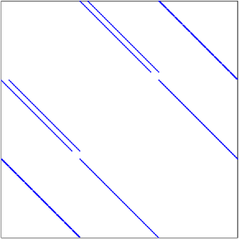
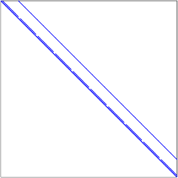
Figure 1: Sparsity pattern of the discrete curl matrix ${\bf C}$ for a $15\times 10\times 10$ grid. (a) The classical FIT (5). (b) The reordered numbering arrangement according to (35).

The complete-solution procedure briefly involves the following successive numerical stages: preparation of the (possibly complex) permittivity and permeability matrices, construction of the discrete curl matrix, incorporation of the boundary conditions to the material matrices, setting up the excitation vector, assemblage of the system matrix equation for the frequency of interest, successive solution of the obtained sparse system of equation, and at last post-processing of the results for monitoring the field quantities on the desired probes.

3 Matrix-Free Method

The memory limitations for the storage of the system matrix and the associated subspaces prohibit the usage of adequately fine grids for an accurate modeling of electrically-small geometrical complexities. As a remedy, the matrix-free methods do not require explicit storage of the product of matrices in (10). Replacing the Laplace operator $s$ in (10) with the angular frequency $j\omega$, the matrix-free algorithm requires only the application of the linear matrix operator to a vector,

$$\begin{array}[]{ll}\underbrace{\underbrace{{\bf M}_{\varepsilon}^{-1/2}\underbrace{{\bf C}^{\rm T}\underbrace{{\bf M}_{\mu}^{-1}\underbrace{{\bf C}\underbrace{{\bf M}_{\varepsilon}^{-1/2}{\begin{picture}(9.0,12.5)\put(0.0,0.0){\makebox(9.0,12.0)[b]{$\stackrel{{\scriptstyle\begin{picture}(4.0,1.0)\put(0.0,-2.0){$\scriptscriptstyle\smallfrown^{\prime}$} \end{picture}}}{{\rule[0.0pt]{1.0pt}{0.0pt}\bf e}}$}} \end{picture}}}_{{\bf x}^{(1)}}}_{{\bf y^{(1)}}}}_{{\bf x^{(2)}}}}_{{\bf y^{(2)}}}}_{{\bf x^{(3)}}}-\omega^{2}{\bf I}{\begin{picture}(9.0,12.5)\put(0.0,0.0){\makebox(9.0,12.0)[b]{$\stackrel{{\scriptstyle\begin{picture}(4.0,1.0)\put(0.0,-2.0){$\scriptscriptstyle\smallfrown^{\prime}$} \end{picture}}}{{\rule[0.0pt]{1.0pt}{0.0pt}\bf e}}$}} \end{picture}}}_{{\bf y^{(3)}}}=-j\omega{\bf M}_{\varepsilon}^{-1/2}{\begin{picture}(9.0,12.5)\put(0.0,0.0){\makebox(9.0,12.0)[b]{$\stackrel{{\scriptstyle\begin{picture}(4.0,3.0)\put(0.0,-2.0){$\scriptscriptstyle\smallfrown$} \put(0.0,-0.5){$\scriptscriptstyle\smallfrown$} \end{picture}}}{{\rule[0.0pt]{1.0pt}{0.0pt}\bf j}}$}} \end{picture}}\end{array}$$ (37)

where ${\bf I}$ is the identity matrix and $.^{(q)}$ represents the $q^{\rm th}$ reuse of the memory buffers ${\bf x}$ and ${\bf y}$. Thus, properly user-defined shell matrix operations can be applied instead of explicit assemblage of ${\bf A}$, using for example the PETSc matrix operations MatMult() and MatMultTranspose() between three VecPointwiseMult() vector operations plus VecAXPY() for summing up the scalar $-\omega^{2}$ term. Therefore, the matrix-free implementation of the square matrix-vector products in FIT requires only 2 temporary vectors, namely ${\bf x}$ and ${\bf y}$ as (37) implies, and 4 temporary vectors when ${\bf C}$ is non-square due to the possible elimination of null rows.

For preallocation of the sparse parallel matrix ${\bf C}$ via MatCreateMPIAIJ(), the number of nonzeros per row is set to 4. To store ${\bf C}$ with 4 non-zero per line when using a CSR-format, $(4+8)\,4\,n_{e}$ bytes of memory is required for the storage of the integer column indices and the nonzero real values. Indeed, the CSR-format also requires a third array with length $4n_{e}$ (in fact $n_{e}+1$ entries with typically 4 bytes each) pointing to the beginning of each row. This third array does affect the memory consumption here as the average number of nonzeros per row is relatively small. Additionally, two floating-point arrays, each allocating $8n_{e}$ bytes, are needed to store the diagonal elements of the material matrices ${\bf M}_{\varepsilon}^{-1/2}$ and ${\bf M}_{\mu}^{-1}$ in double-precision. Hence, the matrix-free matrices in (37) demands $8\,n_{e}+(4+4+8)\,4\,n_{e}+8\,n_{e}=80\,n_{e}$ bytes of memory to store ${\bf C}$ and diagonals of the material matrices.

The explicit sparse storage of the FIT-system matrix ${\bf A}$ with 13 double-precision entries per line in (10) requires $(4+8)\,13\,n_{e}=156\,n_{e}$ bytes plus the additional $8\,n_{e}$ bytes for saving ${\bf M}_{\varepsilon}^{-1/2}$ needed for the final voltage scaling. Note that the classical FIT (8) or (10) entail the multiplication of 13 non-zero elements in $n_{e}$ rows of the system matrix for every iteration, whereas in (37) only $(1+4+1+4+1)$ entries have to be multiplied per row. Note that the summation of $-\omega^{2}$ term should be added to the operation counts of the matrix free methods.

On the other hand, considering ${\bf A}={\cal A}^{\rm T}\!{\cal A}$ where ${\cal A}={\bf M}_{\mu}^{-1/2}{\bf C}{\bf M}_{\varepsilon}^{-1/2}$ and ${\bf M}_{\mu}^{-1/2}$ represents the root of inverse permeability values, one can construct ${\cal A}$ and alternatively utilize the above-mentioned two shell matrix operations

$$\begin{array}[]{ll}\underbrace{\underbrace{({\bf M}_{\mu}^{-1/2}{\bf C}{\bf M}_{\varepsilon}^{-1/2})^{\rm T}\underbrace{{({\bf M}_{\mu}^{-1/2}{\bf C}{\bf M}_{\varepsilon}^{-1/2})}{\begin{picture}(9.0,12.5)\put(0.0,0.0){\makebox(9.0,12.0)[b]{$\stackrel{{\scriptstyle\begin{picture}(4.0,1.0)\put(0.0,-2.0){$\scriptscriptstyle\smallfrown^{\prime}$} \end{picture}}}{{\rule[0.0pt]{1.0pt}{0.0pt}\bf e}}$}} \end{picture}}}_{\bf t}}_{\bf x}-\omega^{2}{\bf I}{\begin{picture}(9.0,12.5)\put(0.0,0.0){\makebox(9.0,12.0)[b]{$\stackrel{{\scriptstyle\begin{picture}(4.0,1.0)\put(0.0,-2.0){$\scriptscriptstyle\smallfrown^{\prime}$} \end{picture}}}{{\rule[0.0pt]{1.0pt}{0.0pt}\bf e}}$}} \end{picture}}}_{\bf y}.\end{array}$$ (39)

This yields a more efficient algorithm than (37) due to the less vector operations and overwriting ${\cal A}$ on ${\bf C}$ by applying MatDiagonalScale() and deallocating the memory reserved for ${\bf M}_{\mu}^{-1/2}$ shrinks the memory usage to $(4+4+8)\,4\,n_{e}+8\,n_{e}=72\,n_{e}$ bytes. This calls for $(4+4)\,n_{e}$ multiplications per iteration and $2\,n_{e}$ multiplications for the construction of $\cal A$ in advance.

The KSP solvers in PETSc support matrix-free methods. Matrix-free methods efficiently carry out matrix-vector products but the associated iterative solvers do not work well without a preconditioner [13]. Hence, a user-defined preconditioner should be devised [14]. An additional matrix-vector product, however, is not necessarily needed to extract for example the diagonal elements of the shell matrix, as a diagonal preconditioner can be constructed by taking the sum square elements of the columns of the sparse matrix ${\cal A}$, i.e.,

$$[{\cal P}]_{ii}=\!\sum_{k}[{\bf M}_{\mu}^{-1}]_{kk}[{\bf C}]_{ki}^{2}[{\bf M}_{\varepsilon}^{-1}]_{ii}\!=\!\!\sum_{k,j=i}\![{\cal A}]_{ik}^{\rm T}[{\cal A}]_{kj}\!=\!\sum_{k}[{\cal A}]_{ki}^{2}.$$

Table 1 reflects the computational costs and storage demands for the introduced formulations.

Table 1: Comparison of the required element-wise multiplications per iteration and memory consumptions for different types of FIT implementations with $n_{e}$ degrees of freedom.

FIT	Classical		Matrix-Free
Algorithms	(8)	(10)	(37)	(39)
Symmetric	$\times$	$\checkmark$	$\checkmark$	$\checkmark$
Memory Usage	$164\,n_{e}$	$164\,n_{e}$	$80\,n_{e}$	$72\,n_{e}$
Multiplications	$13\,n_{e}$	$13\,n_{e}$	$12\,n_{e}$	$9\,n_{e}$

When an extremely large mesh has to be generated, in the pre-processing stage the simulation domain can simply be decomposed into slices along the $z$-axis to accumulate the information associated with slices of material matrices on different machines. The PETSc provides distributed arrays which can be decomposed along all three axes. The slicing along the $z$-axis is an intuitive option which facilitates the implementation and might not be the optimal domain decomposition. Other options for mesh partitioning are using the METIS or Scotch software packages. The optimal domain decomposition for the Jacoby method is the one which minimizes the surface-to-volume ratio of each submesh owned by an MPI rank [15].

4 Numerical Results and Discussion

The correctness of the code was first checked through eigenmode calculations of rectangular and circular cavities for which analytical solution exists. In the following examples, time-harmonic currents ${\bf i}={\begin{picture}(9.0,12.5)\put(0.0,0.0){\makebox(9.0,12.0)[b]{$\stackrel{{\scriptstyle\begin{picture}(4.0,3.0)\put(0.0,-2.0){$\scriptscriptstyle\smallfrown$} \put(0.0,-0.5){$\scriptscriptstyle\smallfrown$} \end{picture}}}{{\rule[0.0pt]{1.0pt}{0.0pt}\bf j}}$}} \end{picture}}$ are imposed at the input ports as the excitation signal and the voltages ${\bf u}={\bf M}_{\varepsilon}^{-1/2}{\begin{picture}(9.0,12.5)\put(0.0,0.0){\makebox(9.0,12.0)[b]{$\stackrel{{\scriptstyle\begin{picture}(4.0,1.0)\put(0.0,-2.0){$\scriptscriptstyle\smallfrown^{\prime}$} \end{picture}}}{{\rule[0.0pt]{1.0pt}{0.0pt}\bf e}}$}} \end{picture}}$ along the segments of desired probes are summed up as the output values. The relative permeability $\mu_{r}$=1 and zero-conductivity $\sigma=0\;\rm S/m$ are assumed for the material properties, unless otherwise mentioned. A relative decrease to less than $10^{-12}$ in the residual norm is set as the stop criterion for iterative solvers and the internal impedance of the source is assumed $Z_{0}=50\>\Omega$ for s-parameter calculations. The obtained impedance (Z)-parameters of multi-port network devices are compared with CST MICROWAVE STUDIO^® (MWS) transient solver results with discrete face-port excitation. The CST MWS benchmark results are obtained on the same mesh grids used for the presented frequency-domain methods. The presented schemes also cover the usage of higher-order FIT for faster convergence, since only the material matrices would then be affected.

Figure 2: A microstrip line enclosed in a metallic box. For the clarity of representation, the surrounding box was represented as a transparent one.

As the first example, a microstrip line enclosed in a PEC box as depicted in Fig. 2 is analyzed. Fig. 3 illustrates the execution times of different blocks of the program in modeling the microstrip line at a single frequency $f=0.5$ GHz on 96 processors in a distributed memory architecture using the conjugate gradient method. The $x$-axis tick labels represent different stages of the solution process, i.e. respectively, preparation of the discrete curl, permittivity, and permeability matrices, inclusion of boundary conditions in the material matrices, stimulation of excitation ports and assemblage of the frequency-dependant shell system matrix, iterative solution of the obtained system of equations using Krylov subspace methods, determination of observation probes to store the desired part of the solution, and finally the post-processing impedance calculations. As displayed in Fig. 3, the construction of the shell matrix does not take much time in comparison with the KSP solver iterations till convergence.

To study the solver speedup under uniform memory access time on multi-core shared memory processsors, a quad-core 64-bit Intel Xeon X5647 CPU with 12M cache and 24 GB of RAM is considered. The speedup factor reaches to 3 for solving the microstrip line problem with hundred thousand unknowns on 4 cores, that is 75% efficiency, and it falls down to the same efficiency factor 75% on 2 cores due to the memory bandwidth limitations for larger problems with million unknowns.

Figure 3: (a) The timing of different stages of constructing (37) for the problem sketched in Fig. 2 discretized by $849\times 608\times 327$ mesh cells and solving it for $n_{e}$= 506 384 352 unknowns on 96 nodes using the conjugate gradient method. (b) The speedup diagram of solving the matrix equation resulting from (37) for the microstrip line problem depicted in Fig. 2 discretized by $497\times 354\times 193$ mesh cells on clusters of the workstation using the KSP conjugate gradient method. The 8 nodes timing is used as reference.

Fig. 3 demonstrates the speedup factor in solving the obtained linear system of equations using the KSP conjugate gradient method. Fig. 4 compares the elapsed CPU time for solving (37) on 64 nodes for $n_{e}$=10 212 276 unknowns associated with the problem shown in Fig. 2 by different iterative methods provided in PETSc 3.4 [9]. Although the conjugate gradient squared (cgs) method apparently converges faster than the others, its matrix-free implementation does not deliver accurate results close to the resonant frequencies of the large-size problems, and hence, it is excluded from the rest of paper. The generalized minimal residual method (gmres) family have shown to be relatively slow. It seems that the explicitly stored Krylov space generated by Gram-Schmidt orthogonalisation constitutes the overhead for gmres. Note that the flexible gmres (fgmres) is equivalent to gmres as long as the preconditionner is not modified during the iterations. It is also worth noting that the conjugate gradient (cg) method is only applicable if the system matrix ${\bf A}$ is symmetric positive definite (SPD), i.e. if ${\cal A}$ defined before (39) is invertible.

Figure 4: The solution time for different PETSc iterative methods: the biconjugate gradient stabilized (bcgs), conjugate gradient (cg), conjugate gradient squared (cgs), conjugate residual (cr), generalized minimal residual (gmres), flexible gmres (fgmres), two variants of transpose-free quasi-minimal residual (tfqmr and tcqmr) methods.

Fig. 5 demonstrates the balance of workload among the used 96 processors for the solution of $n_{e}$=506 384 352 FIT unknowns using the biconjugate gradient stabilized method. Less than 0.1 second imbalance is observed in the total run time of different processors due to I/O and less than 1.6 MB in the peak memory consumption among the ranks. Note that the execution time and peak memory usage for the construction of material matrices on the first rank has also been included in Fig. 5. Fig. 6 displays the strong scaling (i.e. fixed global problem size) experiment, considering the complete solution time when the problem size is kept fixed $n_{e}$=101 868 102 and solved by the biconjugate gradient stabilized method. Fig. 6 exhibits the weak scaling (i.e. fixed problem size per node) experiment, cosidering the complete solution procedure with the biconjugate gradient stabilized method when the number of unknowns are proportionally scaled with the number of cluster nodes. The iteration counts for different system sizes grow almost linearly.

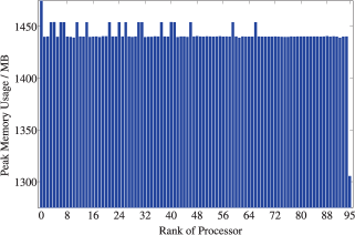
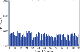
Figure 5: The load-balance in simulation of the microstrip line at $f=0.5$ GHz discretized by $849\times 608\times 327$ mesh cells resulting in $n_{e}$= 506 384 352 unknowns distributed on 96 nodes solved by the biconjugate gradient stabilized method.

Figure 6: (a) The strong scaling experiment with the simulation of the microstrip line at $f=0.5$ GHz for the fixed problem size of $n_{e}$=101 868 102 on a distributed-memory machine using the biconjugate gradient stabilized method. (b) The weak scaling experiment on the simulation of the microstrip line with the help of biconjugate gradient stabilized method for a constant ratio of workload to the used nodes in the cluster.

Figure 7: (a) A four-port coplanar coupler without ground plane. The exact geometrical details can be found in CST-MWS examples [10]. (b) The input impedance $Z_{11}$ and the forward gain $Z_{21}$ for the coplanar coupler shown in Fig. 7.

The correctness of the parallelized matrix-free implementation for the four short-listed robust iterative solvers from Fig. 4, namely the bcgs, cr, cg, and gmres methods, are now investigated on four complex case studies. As another example of planar devices, a four-port coupler consisting of coplanar lines without ground plane planted on a dielectric substrate with the relative permittivity $\epsilon_{r}$=2.7 is considered. The structure is placed up on a $500~{}\mu$m thick aluminium layer as shown in Fig. 7. The thickness of the thin substrate is $13~{}\mu$m. Ports are placed vertically between the striplines and the underlay ground to let the two (even and odd) quasi-TEM modes be able to propagate along the lines. Perfect magnetic conductors (PMC) are considered on all sides of the structure to avoid the excitation of auxiliary box modes. The structured mesh $N_{x}$=46, $N_{y}$=73, $N_{z}$=16 results in $n_{e}$=161 184 degrees of freedom for which (37) is solved at $N_{f}$=200 equidistant frequencies within the range $[f_{\rm min},f_{\rm max}]=[0.26,26]$ GHz using the generalized minimal residual method. As shown in Fig. 7, the matrix-free method (MFM)-FIT results agree well with the CST-MWS time-domain solver results on the same hexahedral mesh. Note that, the present implementation is equipped with the perfect boundary approximation (PBA)^® technique for accurate modeling of curved objects.

The next structure to be analyzed contains two vias for transmitting the signal from one side of the printed circuit board (PCB) to the other side while bridging over a metal barrier, as depicted in Fig. 8. The thickness of the substrate is $1.25$ mm. The PEC boundary condition is considered for all sides of the structure, except the top and bottom sides which are terminated by PMC. The hexahedral mesh $N_{x}=31$, $N_{y}=77$, $N_{z}=22$ gives $n_{e}$=157 542 degrees of freedom in (39). Fig. 8 shows the associated impedances for the frequency range $[f_{\rm min},f_{\rm max}]=[1,7.5]$ GHz obtained using the conjugate gradient method when the ports are placed $2.5$ mm distant from the PEC walls.

Figure 8: (a) A transmission line using strip lines in three dimensions placed on a dielectric substrate. The strip lines on the top surface of the substrate are connected to a short strip line on the bottom surface by small cylinders enabling the bypass of a possible barrier. (b) The input impedance $Z_{11}$ and the forward gain $Z_{21}$ for the microstrip transmission line in Fig. 8.

The next case study is composed of several different materials. An RJ45 connector, consisting of a socket jack and 4 differential pairs of wires for the signal transmission, is analyzed. The wires of the male socket are fixed to a substrate plate, the other wires are connected to a metallic ground plane for shielding purposes, Fig. 9. The thickness of the metal connectors are $0.5$ mm, the substrate thickness is $1$ mm, and the insulator grip thickness is $1.5$ mm. The simulation domain is confined to a $34\times 14\times 11.75~{}\rm mm^{3}$ metallic box. The generated mesh $N_{x}$=63, $N_{y}$=45, $N_{z}$=28 yields to $n_{e}$=238 140 degrees of freedom in (39) which are solved using the KSP conjugate residual method. The discrete port 1 imposes a unit current as the input at the plug end of the connector and the crosstalk voltage along the coupled port 2 at the same side of the connector is shown in Fig. 9.

Figure 9: (a) An RJ45 connector containing 4 pairs of wire conductors and the plastic socket. The model dimensions can be found in CST STUDIO SUITE${}^{\,\rm TM}$ examples. (b) The input impedance $Z_{11}$ and the crosstalk impedance $Z_{21}$ for the connector RJ45 in Fig. 9.

As the final example, a quad flat IC package consisting of a silicon chip with the relative permittivity $\epsilon_{r}$=12.3 encapsulated within a nonconductive plastic compound is simulated. The surface mounted package is concentrically soldered to the PCB with a PEC ground layer, Fig. 10. The thickneParallelss of the metal strips is $0.1$ mm, the substrate thickness is $0.5$ mm, and the plastic thickness is $2.1$ mm. The electric BC is considered for all sides of the $13.4\times 13.4\times 3.075968~{}\rm mm^{3}$ surrounding box. The structured mesh $N_{x}$=65, $N_{y}$=65, $N_{z}$=14 results in $n_{e}$=177 450 degrees of freedom. The discrete port 1 imposes a specific current as the input and (37) is solved for $N_{f}$=200 samples in the frequency range $[f_{\rm min},f_{\rm max}]=[0.06,6]$ GHz using the biconjugate gradient stabilized method. The induced voltage along the port 1 and the coupled voltage along the neighboring pad are read as the outputs. The broadband results shown in Fig. 10 comply with the CST-MWS transient solver results on the same hexahedral mesh. The enormous abstraction of the code in PETSc environment eases the solver modification, for example when mutual field coupling between many ports in Fig. 10 are to be calculated. In fact, one only needs to update the excitation vector on the right hand side of (8) or (10), likewise (37) or (39), by activating all pins of the chip at single run and the solver has not to be run for each single port separately.

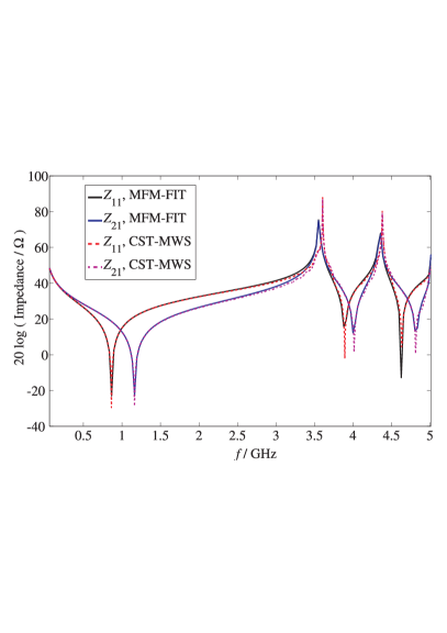
Figure 10: (a) A 52-pin IC package consisting of a silicon chip encapsulated within a nonconductive plastic compound. The model size can be found in CST-MWS examples [10]. (b) The input impedance $Z_{11}$ and the coupling impedance $Z_{21}$ for the IC package in Fig. 10.

5 Conclusions

The matrix-free methods were adopted to the FIT scheme to minimize the number of multiplications and memory requirements in the construction of the final system of linear equations. The matrix-free FIT paves the path for realistic modeling of electrically large-scale radiation problems. The introduced recipe provides extreme ease of modifications in the kernel of the applied algorithm, when material tensors are diagonal which is the case in most practical applications with isotropic materials. Initial index reordering of the unknowns was applied to make the FIT system matrix diagonally dominant. The rearrangement also facilitated the decomposition of large domain into slices for passing the mesh information to different machines in the pre-processing stage. Using the PETSc framework for high-performance computing, the accuracy and efficiency of different KSP solvers on the shell matrix were investigated. The biconjugate gradient stabilized and the conjugate residual methods are shown to be optimal with respect to the solution time among the other alternative iterative solvers for the presented problems with different sizes. Performing large-scale simulations with 1.5 billion unknowns on 64 processors takes about several hours per frequency sample with 6 GB peak memory usage. The method also permitted running 102 millions of unknowns on a shared-memory multiprocessor system in less than half a day.

References

- [1] Y. Shao, Z. Peng, and J. F. Lee, “Full-wave real-life 3-D package signal integrity analysis using nonconformal domain decomposition method,” IEEE Trans. Microw. Theory Tech., vol. 59, no. 2, pp. 230–241, Feb. 2011.
- [2] W. Yu, X. Yang, Y. Liu, and R. Mittra et al., “New development of parallel conformal FDTD method in computational electromagnetics engineering,” IEEE Antennas Propag. Mag., vol. 53, no. 3, pp. 15–41, 2011.
- [3] C. S. Lavranos and G. A. Kyriacou, “Eigenvalue analysis of curved waveguides employing an orthogonal curvilinear frequency-domain finite-difference method,” IEEE Trans. Microw. Theory Tech., vol. 57, no. 3, pp. 594–611, Mar. 2009.
- [4] P. Przybyszewski, “Fast finite difference numerical techniques for the time and frequency domain solution of electromagnetic problems,” Supervised by M. Mrozowski, Technical University of Gdansk, 2001.
- [5] R. Schuhmann and T. Weiland, “Conservation of discrete energy and related laws in the finite integration technique,” Progress In Electromagnetics Research, vol. 32, pp. 301–316, 2001.
- [6] E. Gjonaj, T. Weiland, I. Munteanu, and P. Thoma, “A parallel electromagentic simulation approach for the signal integrity analysis of IC packages,” in Proc. IEEE Int. Electromagn. Compat. Symp. (EMC’07), Honolulu, HI, 2007, pp. 1–5.
- [7] T. Ren, T. Kalscheuer, S. Greenhalgh, and H. Maurer, “Boundary element solutions for broadband 3D geo-electromagentic problems accelerated by multi-level fast mutlipole method,” Int. J. Geophys., vol. 192, no. 2, pp. 473–499, Feb. 2013.
- [8] T. Iwashita, Y. Hirotani, T. Mifune, T. Murayama, and H. Ohtani, “Large-scale time-harmonic electromagnetic field analysis using a multigrid solver on a distributed memory parallel computer,” Parallel Computing, vol. 38, no. 9, pp. 485–500, Sep. 2012.
- [9] S. Balay, J. Brown, K. Buschelman, V. Eijkhout, W. Gropp, D. Kaushik, M. Knepley, L. C. McInnes, B. Smith, and H. Zhang, PETSc Users Manual Revision 3.4, Argonne, IL, May 2013.
- [10] “CST STUDIO SUITE 2013,” CST - Computer Simulation Technology AG, Bad Nauheimer Str. 19, 64289 Darmstadt, Germany, Tech. Rep., 2013.
- [11] M. Clemens and T. Weiland, “Discrete electromagnetism with the finite integration technique,” Progress In Electromagnetics Research, vol. 32, pp. 65–87, 2001.
- [12] R. C. Rumpf, C. R. Garcia, E. A. Berry, and J. H. Barton, “Finite-difference frequency-domain algorithm for modeling electromagnetic scattering from general anisotropic objects,” Progress In Electromagnetics Research B, vol. 61, pp. 55–67, 2014.
- [13] W. Shin, “3D finite-difference frequency-domain method for plasmonics and nanophotonics,” Ph.D. dissertation, Stanford University, 2013.
- [14] A. Chabory, B. de Hon, W. Schilders, and A. Tijhuis, “Preconditioned finitedifference frequency-domain for modelling periodic dielectric structures - comparisons with fdtd,” in Proc. 38th European Microwave Conf. (EuMC’08), Amsterdam, the Netherlands, Oct 2008.
- [15] G. Hager and G. Wellein, Introduction to High Performance Computing for Scientists and Engineers, 1st ed. CRC Press, Taylor & Francis Group, 2011.