Experimental status of the nuclear spin scissors mode

Abstract

With the Wigner Function Moments (WFM) method the scissors mode of the actinides and rare earth nuclei are investigated. The unexplained experimental fact that in ²³²Th a double hump structure is found finds a natural explanation within WFM. It is predicted that the lower peak corresponds to an isovector spin scissors mode whereas the higher lying states corresponds to the conventional isovector orbital scissors mode. The experimental situation is scrutinized in this respect concerning practically all results of $M1$ excitations.

I Introduction

In a recent paper BaMo the Wigner Function Moments (WFM) or phase space moments method was applied for the first time to solve the TDHF equations including spin dynamics. As a first step, only the spin orbit interaction was included in the consideration, as the most important one among all possible spin dependent interactions because it enters into the mean field. The most remarkable result was the prediction of a new type of nuclear collective motion: rotational oscillations of ”spin-up” nucleons with respect of ”spin-down” nucleons (the spin scissors mode). It turns out that the experimentally observed group of peaks in the energy interval $2-4$ MeV corresponds very likely to two different types of motion: the orbital scissors mode and this new kind of mode, i.e. the spin scissors mode. The pictorial view of these two intermingled scissors is shown in Fig. 1. It just shows the generalization of the classical picture for the orbital scissors (see, for example, Lo2000 ; Heyd ) to include the spin scissors modes.

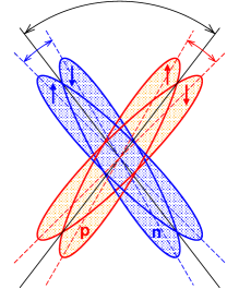
Figure 1: (Color online) Pictorial representation of two intermingled scissors: the orbital scissors (neutrons versus protons) + spin scissors (spin-up nucleons versus spin-down nucleons). Arrows inside of ellipses show the direction of spin projections. p – protons, n – neutrons.

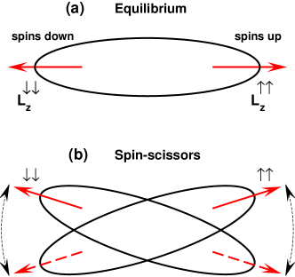
Figure 2: (Color online) (a) Protons with spins $\uparrow$ (up) and $\downarrow$ (down) having nonzero orbital angular momenta at equilibrium. (b) Protons from Fig.(a) vibrating against one-another.

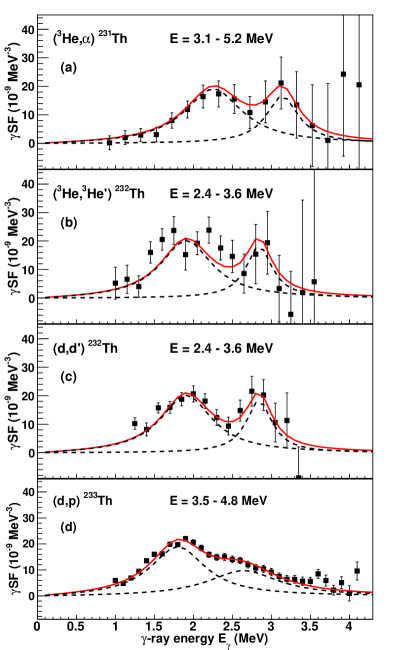
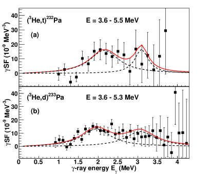
Figure 3: (Color online) Radiative Strength Functions (RSF) for scissors resonance observed by Oslo group Siem2 for ^231-233Th and ^232-233Pa. This figure is taken from the paper Siem2 .

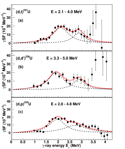
Figure 4: (Color online) Same as Fig. 3 for ^237-239U. This figure is taken from the paper Siem2 .

In Ref. BaMoPRC the influence of the spin-spin interaction on the scissors modes was studied. It was found that such interaction does not push the predicted mode strongly up in energy. It turned out that the spin-spin interaction does not change the general picture of the positions of excitations described in BaMo pushing all levels up proportionally to its strength without changing their order. The most interesting result concerns the $B(M1)$ values of both scissors – the spin-spin interaction strongly redistributes $M1$ strength in favour of the spin scissors mode without changing their summed strength.

A generalization of the WFM method which takes into account spin degrees of freedom and pair correlations simultaneously was outlined in BaMoPRC2 , where the rare earth nuclei were considered. As a result the agreement between theory and experiment in the description of nuclear scissors modes was improved considerably. The decisive role in the substantial improvement of results is played by the anti-aligned spins BaMoPRC2 . It was shown that the ground state nucleus consists of two equal parts having nonzero angular momenta with opposite directions, which compensate each other resulting in the zero total angular momentum. This is graphically depicted in Fig. 2(a). On the other hand, when the opposite angular momenta become tilted, one excites the system and the opposite angular momenta are vibrating with a tilting angle, see Fig. 2(b). It is rather obvious from Fig. 2 that these tilted vibrations happen separately in each of the neutron and proton lobes. These spin-up against spin-down motions certainly influence the excitation of the spin scissors mode.

The aim of the present paper is to find the experimental confirmation of our prediction: the splitting of low lying ($E<4$ MeV) $M1$ excitations in two groups corresponding to spin and orbital scissors, the spin scissors being lower in energy and stronger in transition probability $B(M1)$. It turns out that a similar phenomenon was observed and discussed by experimentalists already at the beginning of the ”scissors era”. For example, we cite from the paper of C. Wesselborg et al. Wessel : ”The existence of the two groups poses the question whether they arise from one mode, namely from scissors mode, or whether we see evidence for two independent collective modes.” We already touched this problem in the paper BaMoPRC , where we have found, that our theory explains quite naturally the experimental results of Oslo group Siem for ²³²Th.

We, therefore, will concentrate to a large extent on the explanation of the experiments in the actinides, see Sec. II. In Sec. III, we will try to see whether in the rare earth nuclei there are also signs of a double hump structure. In Sec. IV we will give our conclusions. The description of the WFM method and mathematical details are given in Appendix A.

II The situation in the actinides

Guttormsen et al Siem have studied deuteron and ³He-induced reactions on ²³²Th and found in the residual nuclei ^231,232,233Th and ^232,233Pa ”an unexpectedly strong integrated strength of $B(M1)=11-15~{}\mu_{N}^{2}$ in the $E_{\gamma}=1.0-3.5$ MeV region”. The $B(M1)$ force in most nuclei shows evident splitting into two Lorentzians. ”Typically, the experimental splitting is $\Delta\omega_{M1}\sim 0.7$ MeV, and the ratio of the strengths between the lower and upper resonance components is $B_{L}/B_{U}\sim 2$”. Seeing this obvious splitting the question is raised: ”What is the nature of the splitting?” Their attempt to explain the splitting by a $\gamma$-deformation has failed.

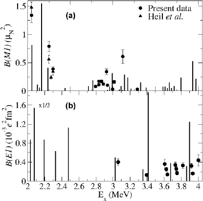
Figure 5: Comparison of experimental and calculated $B(M1)$ (panel (a)) in ²³²Th. Heil et al Heil . The solid line represents QRPA calculations Kuliev . This figure is taken from the paper Adekola ; only panel (a) is necessary for us.

To describe the observed value of $\Delta\omega_{M1}$ the deformation $\gamma\sim 15^{\circ}$ is required, that leads to the ratio $B_{L}/B_{U}\sim 0.7$ in an obvious contradiction with experiment. The authors conclude that ”the splitting may be due to other mechanisms”. Later Siem2 they reanalyzed their data for Th and Pa with the result shown in Fig. 3 and presented the results of new experiments for ^237-239U (Fig. 4) with the conclusion: ”The SR (Scissors Resonance) displays a double-hump structure that is theoretically not understood.”

Table 1: Scissors modes energies $E$ and transition probabilities $B(M1)$. WFM – the results of our calculations for ²³²Th are compared with experimental data: Exp.^c – Ref. Adekola , Exp.^h – Ref. Siem2 .

232Th	$E$ (MeV)				$B(M1)\ (\mu_{N}^{2})$
	WFM	Exp.c	Exp.h		WFM	Exp.c	Exp.h
spin sc.	2.30	2.15	1.95	spin sc.	2.40	2.52(26)	6.5
orb. sc.	2.93	2.99	2.85	orb. sc.	1.42	1.74(38)	3.0
$\Delta E$	0.63	0.84	0.8	$B_{L}/B_{U}$	1.69	1.45	2.2
$E_{\rm cent}$	2.54	2.49	2.2	$B_{\Sigma}$	3.82	4.26(64)	9.5

When the paper BaMoPRC with our explanation of the two humps nature of SR was published, P. von Neumann-Cosel attracted our attention to the paper by A. S. Adekola et al Adekola who have studied the scissors mode in the ($\gamma,\gamma^{\prime}$) reaction on the same nucleus ²³²Th one year earlier. It turns out that these authors have also obtained the scissors mode splitting (see Fig. 5), but did not pay further attention to it.

Figure 6: (Color online) The experimentally observed spectra of $1^{+}$ excitations: (a)²³²Th – Adekola , (b)²³⁶U – U236 , (c)²³⁸U – Hammo . The point of the division of the spectrum in two parts is shown by a blue arrow.

Table 2: Energy centroids $E$ and summed transition probabilities $B(M1)$ of the spin and orbital scissors. Experimental data: ²³²Th – Adekola , ²³⁶U – U236 , ²³⁸U – Hammo . The information for ²³⁶U contains second line, which is obtained by taking into account $1^{+}$ states together with $1^{\pi}$ states with $\pi$ unknown.

Nuclei	$E$ (MeV)						$B(M1)\ (\mu_{N}^{2})$
	spin scissors		orbital scissors		centroid		spin scissors		orbital scissors		$\sum$
	Exp.	WFM	Exp.	WFM	Exp.	WFM	Exp.	WFM	Exp.	WFM	Exp.	WFM
232Th	2.15	2.30	2.99	2.93	2.49(37)	2.54	2.52(26)	2.40	1.74(38)	1.42	4.26(64)	3.82
236U	2.10	2.33	2.61	2.96	2.33	2.57	2.01(25)	2.83	1.60(26)	1.73	3.61(51)	4.56
	2.12		2.63		2.35		2.26(29)		1.80(31)		4.06(60)
238U	2.19	2.36	2.76	3.00	2.58	2.61	2.46(31)	3.18	5.13(89)	2.02	7.59(1.20)	5.20

The energy and $B(M1)$ values of the two humps of SR are shown in Table 1. As it is seen, two experiments Siem2 ; Adekola demonstrate very good agreement in the description of the splitting: $\Delta E$ and $B_{L}/B_{U}$. The big difference in $B(M1)$ values is explained by the fact that in Oslo method one extracts the scissors mode from strongly excited (heated) nuclei, whereas in ($\gamma,\gamma^{\prime}$) reactions one deals with SR in cold (ground state) nuclei. WFM method describes small amplitude deviations from the ground state, so our results must be closer to that of ($\gamma,\gamma^{\prime}$) experiment that is confirmed in Table 1. It is easy to see that the calculated energies $E$ and $B(M1)$ values of the spin and orbital scissors are in very good agreement with the experimental Adekola energy centroids and summarized $B(M1)$ values of the lower and higher groups of levels respectively. Figure 5 contains also the results of QRPA calculations of Kuliev et al Kuliev which are also very intreaguing. As in the experimental works they find a bunch of low-lying states in the region $2.0-2.3$ MeV and a second one in the region $2.7-3.4$ MeV. They also find a third bunch close to 4 MeV. Those results are very similar to ours in what concerns the two low lying structures. It is very tempting to identify their low lying structure with the spin scissors and the second structure with the orbital one. However, the authors did not investigate their structures in those terms. Indeed in an QRPA calculation it is not evident to analyze what is spin and what orbital scissors mode.

It is necessary to stress that the solution of the set of dynamical equations (A.3) gives only two low lying eigenvalues, which are interpreted as the centroid energies of the spin scissors and the orbital scissors according to collective variables responsible for the generation of these eigenvalues (see, for example, Table I of our paper BaMoPRC ). That is why we can compare the results of our calculations (two eigenvalues) only with the equivalent centroids of the experimental scissors spectra.

The experimental spectra of $1^{+}$ excitations obtained in $(\gamma,\gamma^{\prime})$ reactions for three actinide nuclei Adekola ; U236 ; Hammo are shown on Fig. 6. The spectrum of ²³²Th can be divided in two groups with certainty. The division of spectra in two uranium nuclei is not so obvious. For example, there are four variants to divide the spectrum of ²³⁶U in two groups: 1) to put the border (between two groups) into the energy interval $1.80\leq E\leq 2.04$ MeV, 2) or into the interval $2.30\leq E\leq 2.41$ MeV, 3) or $2.51\leq E\leq 2.69$ MeV, 4) or $2.78\leq E\leq 2.95$ MeV. Which interval to choose? To exclude any arbitrariness in the choice of the proper interval, we apply a simple technical device. We folded the experimental spectra with a Lorentzian of increasing width. The width was increased until only two humps remained (see Fig. 7). The blue arrows indicate the position of the minimum between the two humps. We want to stress the fact that the arrows are close to the position where the minima at finite temperature occur for ²³²Th and ²³⁸U. This gives some credit to our method to divide the spectra even at zero temperature into two humps, since it can be expected that if there is a two hump structure at finite temperature, there should be a similar one also at zero temperature.

Figure 7: (Color online) The experimentally observed spectrum of $1^{+}$ excitations of ²³⁶U – U236 is divided in two parts with the help of Lorentzian. The point of the division (the point of minimum between two humps) is shown by a blue arrow. The artificial widths of the spectrum lines used for folding in the case (a) are smaller than the artificial widths used in the case (b).

Figure 8: (Color online) The centroids of experimentally observed spectra of $1^{+}$ excitations in ²³²Th (a) and ²³⁶U (b) (black rectangles with error bars) are compared with the results of calculations (red rectangles) of the spin and orbital scissors modes. In ²³⁶U, the theoretical results are slightly displaced to higher energy with respect to experiment.

Fig. 7 demonstrates the results of folding of ²³⁶U spectrum with smaller (a) and bigger (b) values of the width of the Lorentzian. It is seen that the spectrum of ²³⁶U can eventually be represented by a two-humps curve. Applying this procedure to ²³²Th and ²³⁸U we get the results presented in Table 2. The points of the spectra division are shown on Fig. 6 by blue arrows. The Table 2 demonstrates rather good agreement between the theory and experiment for both scissors in ²³²Th; the agreement in ²³⁶U can be characterized as acceptable. The situation is graphically displayed in Fig. 8. One observes an unexpectedly large value of the summed $B(M1)$ for ²³⁸U in comparison with that of ²³⁶U and ²³²Th and with the theoretical result. The possible reason of this discrepancy was indicated by the authors of Hammo : ”$M1$ excitations are observed at approximately $2.0$ MeV $<E_{\gamma}<3.5$ MeV with a strong concentration of $M1$ states around 2.5 MeV. … The observed $M1$ strength may include states from both the scissors mode and the spin-flip mode, which are indistinguishable from each other based exclusively on the use of the NRF technique.” The most reasonable (and quite natural) place for the boundary between the scissors mode and the spin-flip resonance is located in the spectrum gap between 2.5 MeV and 2.62 MeV. The summed $M1$ strength of scissors in this case becomes $B(M1)=4.38\pm 0.5\ \mu_{N}^{2}$ in rather good agreement with ²³⁶U and ²³²Th. This value is also not so far from the theoretical result. After dividing in spin and orbital scissors it gives $B(M1)_{\rm or}=1.92\ \mu_{N}^{2}$ in good agreement with the calculated value.

We want to stress again that the folding of spectra with Lorentzians is an artifact to divide a given spectrum into a lower lying and a higher lying group. The ensuing width of the two humps should not be interpreted as a true width. Also the specific choice of a Lorentzian has no significance. We could have chosen as well a Gaussian. Below we will apply exactly the same method for the case of Rare Earth nuclei to divide the spectra into two parts. As we will see, the case of Rare Earth nuclei is much harder but we will try and see. In conclusion, our method of separating the often pretty complex splitting patterns of the $M1$ strength into just two humps is an asumption which derives from our present theoretical description where besides the orbital scissors part, a spin scissors part appears.

It should be noted also that both scissors modes have an underlying orbital nature, because both are generated by the same type of collective variables – by the orbital angular momenta (the variables ${\cal L}_{\lambda\mu}$ in (10) with $\lambda=\mu=1$). All the difference is that the ”orbital” (conventional) scissors are generated by the counter-oscillations of the orbital angular momentum of protons with respect of the orbital angular momentum of neutrons, whereas the ”spin” scissors are generated by the counter-oscillations of the orbital angular momentum of nucleons having the spin projection ”up” with respect of the orbital angular momentum of nucleons having the spin projection ”down”. At the same time, both scissors are strongly sensitive to the influence of the spin part of the magnetic dipole operator (16)

$$\hat{O}_{11}=\frac{\mu_{N}}{\hbar}\sqrt{\frac{3}{4\pi}}\left[g_{s}\hat{S}_{1}+g_{l}\hat{l}_{1}\right].$$ (1)

The Table 3 demonstrates the sensitivity of both scissors to the spin-dependent part of nuclear forces: the moderate constructive interference of the orbital and spin contributions in the case of the spin scissors mode and their very strong destructive interference in the case of the orbital scissors mode.

Table 3: Scissors modes energies $E$ and transition probabilities $B(M1)$ for ²³²Th. The results of calculations with and without the spin part of a dipole magnetic operator (1) ($g_{s}\neq 0$ and $g_{s}=0$ respectively).

	$E$ (MeV)			$B(M1)$ ($\mu_{N}^{2}$)
	spin	orb.	centroid	spin	orb.	$\sum$
$g_{s}\neq 0$	2.30	2.93	2.54	2.40	1.42	3.82
$g_{s}=0$	2.30	2.93	2.87	0.74	7.69	8.43

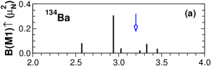
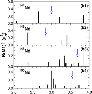
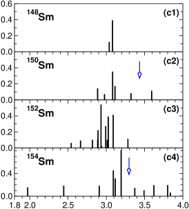
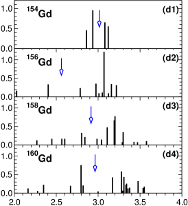
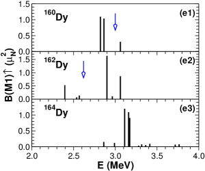
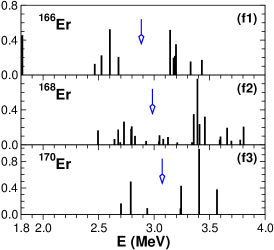
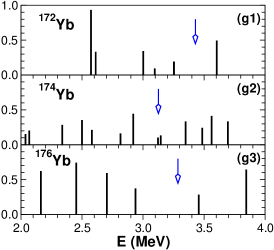
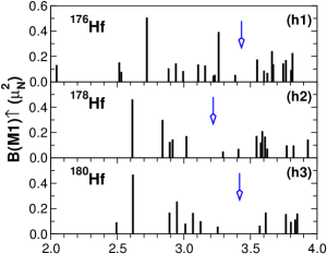
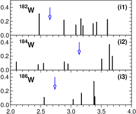
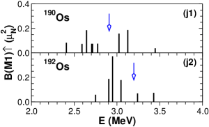
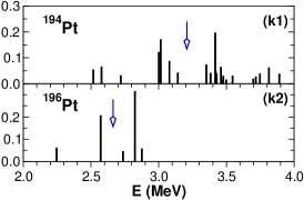
Figure 9: (Color online) The experimentally observed spectra of $1^{+}$ excitations: ¹³⁴Ba – Ba , ^144-150Nd – Nd144 ; Margr , ^148-154Sm – Sm , ^154-160Gd – Gd ; Gd160 , ^160-164Dy – Wessel ; Dy , ^166-170Er – Er , ^172-176Yb – Yb , ^176-180Hf – Hf176 ; Hf , ^182-186W – W , ^190-192Os – Os , ^194-196Pt – Pt194 ; Pt196 . The point of the division of the spectrum in two parts is shown by a blue arrow.

Table 4: Energy centroids $E$ and summed transition probabilities $B(M1)$ of the spin and orbital scissors; spectra are taken from papers shown in the last column. The information for many nuclei contains second line, which is obtained by taking into account $1^{+}$ states together with $1^{\pi}$ states whith $\pi$ unknown.

Nuclei	$E$ (MeV)						$B(M1)\ (\mu_{N}^{2})$						Ref.
	spin scissors		orbital scissors		centroid		spin scissors		orbital scissors		$\sum$
	Exp.	WFM	Exp.	WFM	Exp.	WFM	Exp.	WFM	Exp.	WFM	Exp.	WFM
134Ba	2.88	3.02	3.35	3.43	2.99	3.04	0.43(06)	0.65	0.13(03)	0.03	0.56(09)	0.68	Ba
	2.85		3.65		3.33		0.51(08)		0.76(16)		1.26(24)
144Nd	2.57	2.97	3.57	3.32	3.07	3.21	0.39(03)	0.06	0.39(02)	0.14	0.78(05)	0.20	Nd144
	2.63		3.64		3.22		0.51(05)		0.70(06)		1.21(11)
146Nd	2.36	3.00	3.37	3.38	2.90	3.20	0.34(04)	0.27	0.39(06)	0.30	0.73(10)	0.57	Margr
	2.38		3.60		3.28		0.38(05)		1.08(18)		1.45(23)
148Nd	3.22	3.09	3.83	3.54	3.40	3.22	0.80(19)	0.91	0.32(07)	0.37	1.12(26)	1.28	Margr
150Nd	3.02	2.90	3.72	3.64	3.12	3.13	1.56(21)	1.27	0.27(05)	0.56	1.83(26)	1.83	Margr
148Sm	–	2.98	–	3.35	3.07	3.17	–	0.22	–	0.24	0.51(12)	0.46	Sm
150Sm	3.07	3.06	3.73	3.49	3.18	3.17	0.81(12)	0.84	0.16(05)	0.27	0.97(17)	1.12	Sm
152Sm	–	2.71	–	3.53	2.97	2.99	–	1.65	–	0.85	2.41(33)	2.50	Sm
154Sm	2.98	2.79	3.62	3.64	3.14	3.10	2.08(30)	2.12	0.68(20)	1.22	2.76(50)	3.34	Sm
154Gd	2.91	2.75	3.10	3.58	3.00	3.04	1.40(25)	1.95	1.20(25)	1.05	2.60(50)	3.00	Gd
156Gd	2.28	2.79	3.06	3.63	2.94	3.09	0.49(12)	2.19	2.73(56)	1.24	3.22(68)	3.44	Gd
158Gd	2.64	2.78	3.20	3.62	3.04	3.09	1.13(23)	2.25	2.86(42)	1.27	3.99(65)	3.52	Gd
160Gd	2.65	2.82	3.33	3.67	3.10	3.14	1.53(14)	2.53	2.88(40)	1.49	4.41(54)	4.02	Gd160
160Dy	2.84	2.78	3.06	3.61	2.87	3.08	2.12(25)	2.30	0.30(05)	1.30	2.42(30)	3.60	Wessel
162Dy	2.44	2.78	2.96	3.60	2.84	3.07	0.71(05)	2.37	2.59(19)	1.32	3.30(24)	3.69	Dy
164Dy	–	2.77	–	3.60	3.17	3.07	–	2.44	–	1.36	3.85(31)	3.80	Dy
166Er	2.36	2.77	3.21	3.59	2.79	3.06	1.52(34)	2.48	1.60(24)	1.38	3.12(58)	3.86	Er
	2.37		3.25		2.85		1.56(35)		1.86(46)		3.42(81)
168Er	2.72	2.77	3.43	3.58	3.21	3.06	1.21(14)	2.54	2.63(35)	1.41	3.85(50)	3.95	Er
	2.69		3.46		3.22		1.35(17)		3.04(44)		4.38(61)
170Er	2.79	2.76	3.39	3.57	3.22	3.05	0.75(11)	2.60	1.88(28)	1.43	2.63(39)	4.03	Er
	2.77		3.42		3.21		1.07(19)		2.24(41)		3.30(59)
172Yb	2.75	2.72	3.60	3.51	2.93	2.99	1.88(37)	2.46	0.49(12)	1.26	2.37(49)	3.72	Yb
	2.77		3.73		3.07		1.99(41)		0.94(26)		2.93(67)
174Yb	2.56	2.72	3.49	3.50	2.96	2.98	1.89(70)	2.51	1.44(51)	1.29	3.33(1.21)	3.80	Yb
	2.35		3.29		2.97		1.19(52)		2.28(76)		3.47(1.28)
176Yb	2.52	2.68	3.73	3.44	2.86	2.92	2.32(60)	2.34	0.92(45)	1.12	3.24(1.05)	3.46	Yb
	2.52		3.65		2.98		2.32(60)		1.60(70)		3.92(1.30)
176Hf	2.89	3.06	3.70	3.73	3.22	3.27	1.99(15)	2.15	1.33(13)	1.00	3.32(28)	3.15	Hf176
	2.91		3.69		3.25		2.47(22)		1.93(23)		4.40(45)
178Hf	2.79	3.05	3.64	3.72	3.21	3.27	1.19(11)	2.18	1.19(22)	1.02	2.38(33)	3.20	Hf
	2.73		3.67		3.15		1.19(11)		1.38(26)		2.57(37)
180Hf	2.84	3.02	3.75	3.67	3.16	3.22	1.38(17)	1.97	0.75(13)	0.86	2.13(30)	2.84	Hf
	2.84		3.80		3.30		1.57(22)		1.43(27)		3.00(49)
182W	2.47	2.96	3.25	3.57	3.10	3.13	0.31(05)	1.48	1.34(23)	0.55	1.65(28)	2.03	W
184W	2.58	2.94	3.62	3.52	3.19	3.08	0.51(10)	1.27	0.73(27)	0.41	1.24(37)	1.68	W
186W	2.56	2.91	3.29	3.48	3.19	3.03	0.11(01)	1.06	0.71(20)	0.29	0.82(21)	1.36	W
	2.56		3.36		3.29		0.11(01)		1.18(64)		1.29(65)
190Os	2.64	2.87	3.11	3.25	2.83	2.98	0.56(08)	1.01	0.38(04)	0.38	0.94(12)	1.39	Os
	2.14		3.37		2.72		1.26(19)		1.12(16)		2.38(36)
192Os	2.95	2.85	3.34	3.21	3.00	2.94	0.79(04)	0.74	0.14(02)	0.25	0.93(06)	0.99	Os
	2.89		3.40		3.07		1.16(08)		0.63(06)		1.78(14)
194Pt	2.92	2.82	3.52	3.16	3.25	2.97	0.57(09)	0.66	0.74(14)	0.52	1.31(23)	1.17	Pt194
	2.92		3.51		3.29		0.57(09)		0.93(17)		1.50(25)
196Pt	2.50	2.81	2.82	3.12	2.70	2.95	0.27(05)	0.46	0.42(07)	0.40	0.69(13)	0.86	Pt196
	2.50		2.93		2.79		0.27(05)		0.55(15)		0.82(20)

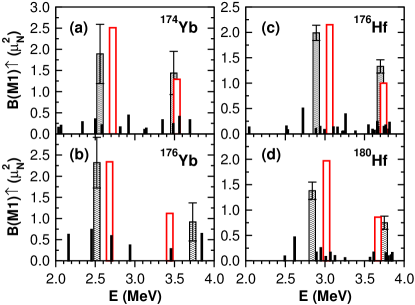
Figure 10: (Color online) The centroids of experimentally observed spectra of $1^{+}$ excitations in ^174,176Yb (a, b) and ^176,180Hf (c, d) (black rectangles with error bars) are compared with the results of calculations (red rectangles) of the spin and orbital scissors modes. Notice that the strength of the lower peak (spin-scissors) is always stronger than the one of the upper peak (orbital-scissors).

III Experimental situation in rare earths

We here will perform a systematic analysis of experimental data for rare earth nuclei, where the majority of nuclear scissors are found. We have studied practically all papers containing experimental data for low lying $M1$ excitations in rare earth nuclei. For the sake of convenience we have collected in Fig. 9 all experimentally known spectra of low lying $1^{+}$ excitations Wessel ; Ba ; Nd144 ; Margr ; Sm ; Gd ; Gd160 ; Dy ; Er ; Yb ; Hf176 ; Hf ; W ; Os ; Pt194 ; Pt196 . It should be emphasized, that only the levels with positive parities are displayed here. As a matter of fact, there exist many $1^{\pi}$ excitations in the energy interval 1 MeV$-4$ MeV, whose parities $\pi$ are not known up to now.

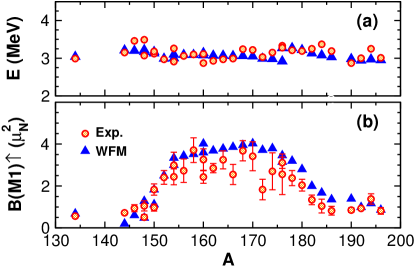
Figure 11: (Color online) Calculated (WFM) mean excitation energies (a) and summed $M1$ strengths (b) of the scissors mode are compared with experimental data (Exp.) from Rich .

One glance on Fig. 9 is enough to understand that the situation with spectra in rare earth nuclei iscomplicated. Nevertheless, we will try to proceed in the same way as with the Actinides: we fold the spectra with a Lorentzian whose width is increased until only two humps survive. The minimum between the two humps is indicated with an arrow in Fig. 9. The states in the low lying group are then identified as belonging to the spin scissors motion and the ones of high lying group as orbital scissors states. The values of $B(M1)$ and energy centroids, corresponding to the described separation, are compared with theoretical results in the Table 4. Studying attentively the Table 4 one can find satisfactory agreement between theoretical and experimental results for the orbital scissors in 13 nuclei: ^146,148Nd, ¹⁵⁴Gd, ^166,170Er, ^174,176Yb, ^176,178,180Hf, ¹⁹⁰Os and ^194,196Pt. The same degree of agreement can be found for the spin scissors in 15 nuclei: ¹³⁴Ba, ^146,148,150Nd, ^150,154Sm, ¹⁵⁴Gd, ¹⁶⁰Dy, ^172,174,176Yb, ^176,180Hf, ¹⁹²Os and ¹⁹⁴Pt. Therefore the satisfactory agreement between theoretical and experimental results for both, the orbital and spin scissors, is observed in 8 nuclei: ^146,148Nd, ¹⁵⁴Gd, ^174,176Yb, ^176,180Hf and ¹⁹⁴Pt. Again, as in Fig. 8 for the Actinides, in Fig. 10 we compare for four rare earth nuclei the experimental centroids with our results. The agreement is nearly perfect. In the other four nuclei the agreement is less good but still acceptable. The harvest seems to be rather meager. However, we have to remember that spin and orbital scissors are surely mostly not quite separated. It is a lucky accident when they are clearly separated like in the Th and (eventually) in Pa isotopes and here as in Fig. 10 .

Therefore, an additional handful of nuclei in the rare earth region is a very welcome support of our theoretical analysis of the existence of two separate sissors modes: spin and orbital. This the more so as we get at least semi-quantitative agreement between experiment and theory, in the sense that for all those selected nuclei the transition probability for spin scissors is stronger than for orbital scissors. This finding gives support to our theoretical analysis. It is worth noting at the end of this section, that sums of experimental $B(M1)$ values and the respective energy centroids agree (with rare exceptions) very well with theoretical predictions (see Fig. 11).

IV Conclusions and Outlook

The aim of this paper was to find experimental indications about the existence of the ”spin” scissors mode predicted in our previous publications BaMo ; BaMoPRC ; BaMoPRC2 . To this end we have performed a detailed analysis of experimental data on $1^{+}$ excitations for actinides and for Rare Earth nuclei of the $N=82-126$ major shell.

First of all let us again comment on the very clear experimental situation in the actinides for heated nuclei of Th, Pa, U isotopes. In all cases a clear two humps structure has been revealed, see Figs. 3 and 4. Unfortunately with our WFM technique, we are so far not prepared to investigate nuclei at finite temperature. So we tried in this work to investigate scissors modes on top of the ground states. We tried to be as exhaustive in the presentation of published data in rare earth nuclei and the actinides as possible. For the actinides, there exists a very clear cut example given by ²³²Th, see Figs. 5 and 6, and our results are in good agreement with the experimental values for position and $B(M1)$ values. We stress again that this concerns also the feature that the $B(M1)$’s are stronger for the hypothetical spin scissors than for the orbital one. For the Uranium isotopes the separation into two peaks of the $M1$ excitations is not so clear. So we tried to find signatures of splitting also in the rare earth nuclei. Despite of the fact that one can imagine that spin-scissors and orbital ones are not well separated in nuclei, lighter than the actinides, we nevertheless found a handful of examples where our method of separation into a high lying and low lying group works and yields satisfying agreement with experiment. Here we again found that $B(M1)$’s are stronger for low lying than for high lying part of levels. So, there are about half a dozen examples which support our theoretical findings that there exist two groups of scissors modes, the spin scissors and orbital scissors modes. Actually we divided the experimental spectra of almost all rare earth nuclei shown in Fig. 9 into low lying and higher lying parts indicated by the blue arrows. Without giving quantitative agreement with experiment besides for those 8 nuclei mentioned in the main text, we at least found most of the time that the low lying parts have stronger $B(M1)$’s than high lying groups again in qualitative agreement with our theoretical investigation. In conclusion, there seems to exist as well some support of the rare earth nuclei for the existence of the spin scissors mode. Let us mention again that we obtained the two hump structures in folding the spectra with a Lorentzian (we also could have taken as well a Gaussian). This method of separating the often quite complex splitting patterns of the $M1$ strength in just two humps is an assumption that derives from the present theoretical description where besides the orbital scissors part, a spin-scissors part appears. A special mention may need the clear situation in ²³²Th because there exists a QRPA calculation Kuliev . This QRPA calculation also reveals a two hump structure in close agreement with experiment and with our findings. We may finish off with the remark that it does not seem evident to disentangle a QRPA spectrum into spin and orbital scissors states. For this it will be necessary to find the excitation operators which specifically excite the spin and orbital scissors individually. For the moment this task can only be achieved with our WFM method because the amplitudes have a clear connection to the physics of the obtained states. It will be a future project to make detailed comparison between the QRPA and our calculations. A further aim is to introduce finite temperature into the WFM formalism what eventually would allow to explain the strongly enhanced $B(M1)$ transitions found experimentally in the Actinides.

Appendix A WFM method and details of calculations

The basis of our method is the Time-Dependent Hartree–Fock–Bogoliubov (TDHFB) equation in matrix formulation Ring :

$$i\hbar\dot{\cal R}=[{\cal H},{\cal R}]$$ (2)

with

$${\cal R}={\hat{\rho}\qquad-\hat{\kappa}\choose-\hat{\kappa}^{\dagger}\;\;1-\hat{\rho}^{*}},\quad{\cal H}={\hat{h}\quad\;\;\hat{\Delta}\choose\hat{\Delta}^{\dagger}\quad-\hat{h}^{*}}$$ (3)

The normal density matrix $\hat{\rho}$ and Hamiltonian $\hat{h}$ are hermitian whereas the abnormal density $\hat{\kappa}$ and the pairing gap $\hat{\Delta}$ are skew symmetric: $\hat{\kappa}^{\dagger}=-\hat{\kappa}^{*}$, $\hat{\Delta}^{\dagger}=-\hat{\Delta}^{*}$.

The detailed form of the TDHFB equations is

$$i\hbar\dot{\hat{\rho}}=\hat{h}\hat{\rho}-\hat{\rho}\hat{h}-\hat{\Delta}\hat{\kappa}^{\dagger}+\hat{\kappa}\hat{\Delta}^{\dagger},$$

$$-i\hbar\dot{\hat{\rho}}^{*}=\hat{h}^{*}\hat{\rho}^{*}-\hat{\rho}^{*}\hat{h}^{*}-\hat{\Delta}^{\dagger}\hat{\kappa}+\hat{\kappa}^{\dagger}\hat{\Delta},$$

$$-i\hbar\dot{\hat{\kappa}}=-\hat{h}\hat{\kappa}-\hat{\kappa}\hat{h}^{*}+\hat{\Delta}-\hat{\Delta}\hat{\rho}^{*}-\hat{\rho}\hat{\Delta},$$

$$-i\hbar\dot{\hat{\kappa}}^{\dagger}=\hat{h}^{*}\hat{\kappa}^{\dagger}+\hat{\kappa}^{\dagger}\hat{h}-\hat{\Delta}^{\dagger}+\hat{\Delta}^{\dagger}\hat{\rho}+\hat{\rho}^{*}\hat{\Delta}^{\dagger}.\qquad$$ (4)

We do not specify the isospin indices in order to make formulae more transparent. Let us consider matrix form of (4) in coordinate space keeping spin indices $s,s^{\prime}$ with compact notation $X_{rr^{\prime}}^{ss^{\prime}}\equiv\langle{\bf r},s|\hat{X}|{\bf r}^{\prime},s^{\prime}\rangle$. Then the set of TDHFB equations with specified spin indices reads BaMoPRC2 :

$$i\hbar\dot{\rho}_{rr^{\prime\prime}}^{\uparrow\uparrow}=\int\!d^{3}r^{\prime}(h_{rr^{\prime}}^{\uparrow\uparrow}\rho_{r^{\prime}r^{\prime\prime}}^{\uparrow\uparrow}-\rho_{rr^{\prime}}^{\uparrow\uparrow}h_{r^{\prime}r^{\prime\prime}}^{\uparrow\uparrow}+\hat{h}_{rr^{\prime}}^{\uparrow\downarrow}\rho_{r^{\prime}r^{\prime\prime}}^{\downarrow\uparrow}-\rho_{rr^{\prime}}^{\uparrow\downarrow}h_{r^{\prime}r^{\prime\prime}}^{\downarrow\uparrow}-\Delta_{rr^{\prime}}^{\uparrow\downarrow}{\kappa^{\dagger}}_{r^{\prime}r^{\prime\prime}}^{\downarrow\uparrow}+\kappa_{rr^{\prime}}^{\uparrow\downarrow}{\Delta^{\dagger}}_{r^{\prime}r^{\prime\prime}}^{\downarrow\uparrow}),$$

$$i\hbar\dot{\rho}_{rr^{\prime\prime}}^{\uparrow\downarrow}=\int\!d^{3}r^{\prime}(h_{rr^{\prime}}^{\uparrow\uparrow}\rho_{r^{\prime}r^{\prime\prime}}^{\uparrow\downarrow}-\rho_{rr^{\prime}}^{\uparrow\uparrow}h_{r^{\prime}r^{\prime\prime}}^{\uparrow\downarrow}+\hat{h}_{rr^{\prime}}^{\uparrow\downarrow}\rho_{r^{\prime}r^{\prime\prime}}^{\downarrow\downarrow}-\rho_{rr^{\prime}}^{\uparrow\downarrow}h_{r^{\prime}r^{\prime\prime}}^{\downarrow\downarrow}),$$

$$i\hbar\dot{\rho}_{rr^{\prime\prime}}^{\downarrow\uparrow}=\int\!d^{3}r^{\prime}(h_{rr^{\prime}}^{\downarrow\uparrow}\rho_{r^{\prime}r^{\prime\prime}}^{\uparrow\uparrow}-\rho_{rr^{\prime}}^{\downarrow\uparrow}h_{r^{\prime}r^{\prime\prime}}^{\uparrow\uparrow}+\hat{h}_{rr^{\prime}}^{\downarrow\downarrow}\rho_{r^{\prime}r^{\prime\prime}}^{\downarrow\uparrow}-\rho_{rr^{\prime}}^{\downarrow\downarrow}h_{r^{\prime}r^{\prime\prime}}^{\downarrow\uparrow}),$$

$$i\hbar\dot{\rho}_{rr^{\prime\prime}}^{\downarrow\downarrow}=\int\!d^{3}r^{\prime}(h_{rr^{\prime}}^{\downarrow\uparrow}\rho_{r^{\prime}r^{\prime\prime}}^{\uparrow\downarrow}-\rho_{rr^{\prime}}^{\downarrow\uparrow}h_{r^{\prime}r^{\prime\prime}}^{\uparrow\downarrow}+\hat{h}_{rr^{\prime}}^{\downarrow\downarrow}\rho_{r^{\prime}r^{\prime\prime}}^{\downarrow\downarrow}-\rho_{rr^{\prime}}^{\downarrow\downarrow}h_{r^{\prime}r^{\prime\prime}}^{\downarrow\downarrow}-\Delta_{rr^{\prime}}^{\downarrow\uparrow}{\kappa^{\dagger}}_{r^{\prime}r^{\prime\prime}}^{\uparrow\downarrow}+\kappa_{rr^{\prime}}^{\downarrow\uparrow}{\Delta^{\dagger}}_{r^{\prime}r^{\prime\prime}}^{\uparrow\downarrow}),$$

$$i\hbar\dot{\kappa}_{rr^{\prime\prime}}^{\uparrow\downarrow}=-\hat{\Delta}_{rr^{\prime\prime}}^{\uparrow\downarrow}+\int\!d^{3}r^{\prime}\left(h_{rr^{\prime}}^{\uparrow\uparrow}\kappa_{r^{\prime}r^{\prime\prime}}^{\uparrow\downarrow}+\kappa_{rr^{\prime}}^{\uparrow\downarrow}{h^{*}}_{r^{\prime}r^{\prime\prime}}^{\downarrow\downarrow}+\Delta_{rr^{\prime}}^{\uparrow\downarrow}{\rho^{*}}_{r^{\prime}r^{\prime\prime}}^{\downarrow\downarrow}+\rho_{rr^{\prime}}^{\uparrow\uparrow}\Delta_{r^{\prime}r^{\prime\prime}}^{\uparrow\downarrow}\right),$$

$$i\hbar\dot{\kappa}_{rr^{\prime\prime}}^{\downarrow\uparrow}=-\hat{\Delta}_{rr^{\prime\prime}}^{\downarrow\uparrow}+\int\!d^{3}r^{\prime}\left(h_{rr^{\prime}}^{\downarrow\downarrow}\kappa_{r^{\prime}r^{\prime\prime}}^{\downarrow\uparrow}+\kappa_{rr^{\prime}}^{\downarrow\uparrow}{h^{*}}_{r^{\prime}r^{\prime\prime}}^{\uparrow\uparrow}+\Delta_{rr^{\prime}}^{\downarrow\uparrow}{\rho^{*}}_{r^{\prime}r^{\prime\prime}}^{\uparrow\uparrow}+\rho_{rr^{\prime}}^{\downarrow\downarrow}\Delta_{r^{\prime}r^{\prime\prime}}^{\downarrow\uparrow}\right).$$ (5)

This set of equations must be complemented by the complex conjugated equations.

We work with the Wigner transform Ring of equations (5). The relevant mathematical details can be found in BaMoPRC2 ; Malov . We do not write out the coordinate dependence $({\bf r},{\bf p})$ of all functions in order to make the formulae more transparent. We have

$$i\hbar\dot{f}^{\uparrow\uparrow} = i\hbar\{h^{\uparrow\uparrow},f^{\uparrow\uparrow}\}+h^{\uparrow\downarrow}f^{\downarrow\uparrow}-f^{\uparrow\downarrow}h^{\downarrow\uparrow}+\frac{i\hbar}{2}\{h^{\uparrow\downarrow},f^{\downarrow\uparrow}\}-\frac{i\hbar}{2}\{f^{\uparrow\downarrow},h^{\downarrow\uparrow}\}$$

$$- \frac{\hbar^{2}}{8}\{\!\{h^{\uparrow\downarrow},f^{\downarrow\uparrow}\}\!\}+\frac{\hbar^{2}}{8}\{\!\{f^{\uparrow\downarrow},h^{\downarrow\uparrow}\}\!\}+\kappa\Delta^{*}-\Delta\kappa^{*}$$

$$+ \frac{i\hbar}{2}\{\kappa,\Delta^{*}\}-\frac{i\hbar}{2}\{\Delta,\kappa^{*}\}-\frac{\hbar^{2}}{8}\{\!\{\kappa,\Delta^{*}\}\!\}+\frac{\hbar^{2}}{8}\{\!\{\Delta,\kappa^{*}\}\!\}+...,$$

$$i\hbar\dot{f}^{\downarrow\downarrow} = i\hbar\{h^{\downarrow\downarrow},f^{\downarrow\downarrow}\}+h^{\downarrow\uparrow}f^{\uparrow\downarrow}-f^{\downarrow\uparrow}h^{\uparrow\downarrow}+\frac{i\hbar}{2}\{h^{\downarrow\uparrow},f^{\uparrow\downarrow}\}-\frac{i\hbar}{2}\{f^{\downarrow\uparrow},h^{\uparrow\downarrow}\}$$

$$- \frac{\hbar^{2}}{8}\{\!\{h^{\downarrow\uparrow},f^{\uparrow\downarrow}\}\!\}+\frac{\hbar^{2}}{8}\{\!\{f^{\downarrow\uparrow},h^{\uparrow\downarrow}\}\!\}+\bar{\Delta}^{*}\bar{\kappa}-\bar{\kappa}^{*}\bar{\Delta}$$

$$+ \frac{i\hbar}{2}\{\bar{\Delta}^{*},\bar{\kappa}\}-\frac{i\hbar}{2}\{\bar{\kappa}^{*},\bar{\Delta}\}-\frac{\hbar^{2}}{8}\{\!\{\bar{\Delta}^{*},\bar{\kappa}\}\!\}+\frac{\hbar^{2}}{8}\{\!\{\bar{\kappa}^{*},\bar{\Delta}\}\!\}+...,$$

$$i\hbar\dot{f}^{\uparrow\downarrow} = f^{\uparrow\downarrow}(h^{\uparrow\uparrow}-h^{\downarrow\downarrow})+\frac{i\hbar}{2}\{(h^{\uparrow\uparrow}+h^{\downarrow\downarrow}),f^{\uparrow\downarrow}\}-\frac{\hbar^{2}}{8}\{\!\{(h^{\uparrow\uparrow}-h^{\downarrow\downarrow}),f^{\uparrow\downarrow}\}\!\}$$

$$- h^{\uparrow\downarrow}(f^{\uparrow\uparrow}-f^{\downarrow\downarrow})+\frac{i\hbar}{2}\{h^{\uparrow\downarrow},(f^{\uparrow\uparrow}+f^{\downarrow\downarrow})\}+\frac{\hbar^{2}}{8}\{\!\{h^{\uparrow\downarrow},(f^{\uparrow\uparrow}-f^{\downarrow\downarrow})\}\!\}+....,$$

$$i\hbar\dot{f}^{\downarrow\uparrow} = f^{\downarrow\uparrow}(h^{\downarrow\downarrow}-h^{\uparrow\uparrow})+\frac{i\hbar}{2}\{(h^{\downarrow\downarrow}+h^{\uparrow\uparrow}),f^{\downarrow\uparrow}\}-\frac{\hbar^{2}}{8}\{\!\{(h^{\downarrow\downarrow}-h^{\uparrow\uparrow}),f^{\downarrow\uparrow}\}\!\}$$

$$- h^{\downarrow\uparrow}(f^{\downarrow\downarrow}-f^{\uparrow\uparrow})+\frac{i\hbar}{2}\{h^{\downarrow\uparrow},(f^{\downarrow\downarrow}+f^{\uparrow\uparrow})\}+\frac{\hbar^{2}}{8}\{\!\{h^{\downarrow\uparrow},(f^{\downarrow\downarrow}-f^{\uparrow\uparrow})\}\!\}+...,$$

$$i\hbar\dot{\kappa} = \kappa\,(h^{\uparrow\uparrow}+\bar{h}^{\downarrow\downarrow})+\frac{i\hbar}{2}\{(h^{\uparrow\uparrow}-\bar{h}^{\downarrow\downarrow}),\kappa\}-\frac{\hbar^{2}}{8}\{\!\{(h^{\uparrow\uparrow}+\bar{h}^{\downarrow\downarrow}),\kappa\}\!\}$$

$$+ \Delta\,(f^{\uparrow\uparrow}+\bar{f}^{\downarrow\downarrow})+\frac{i\hbar}{2}\{(f^{\uparrow\uparrow}-\bar{f}^{\downarrow\downarrow}),\Delta\}-\frac{\hbar^{2}}{8}\{\!\{(f^{\uparrow\uparrow}+\bar{f}^{\downarrow\downarrow}),\Delta\}\!\}-\Delta+...,$$

$$i\hbar\dot{\kappa}^{*} = -\kappa^{*}(h^{\uparrow\uparrow}+\bar{h}^{\downarrow\downarrow})+\frac{i\hbar}{2}\{(h^{\uparrow\uparrow}-\bar{h}^{\downarrow\downarrow}),\kappa^{*}\}+\frac{\hbar^{2}}{8}\{\!\{(h^{\uparrow\uparrow}+\bar{h}^{\downarrow\downarrow}),\kappa^{*}\}\!\}$$ (6)

$$- \Delta^{*}(f^{\uparrow\uparrow}+\bar{f}^{\downarrow\downarrow})+\frac{i\hbar}{2}\{(f^{\uparrow\uparrow}-\bar{f}^{\downarrow\downarrow}),\Delta^{*}\}+\frac{\hbar^{2}}{8}\{\!\{(f^{\uparrow\uparrow}+\bar{f}^{\downarrow\downarrow}),\Delta^{*}\}\!\}+\Delta^{*}+...,$$

where the functions $h$, $f$, $\Delta$, and $\kappa$ are the Wigner transforms of $\hat{h}$, $\hat{\rho}$, $\hat{\Delta}$, and $\hat{\kappa}$, respectively, $\bar{f}({\bf r},{\bf p})=f({\bf r},-{\bf p})$, $\{f,g\}$ is the Poisson bracket of the functions $f$ and $g$ and $\{\{f,g\}\}$ is their double Poisson bracket. The dots stand for terms proportional to higher powers of $\hbar$ – after integration over phase space these terms disappear and we arrive to the set of exact integral equations. This set of equations must be complemented by the dynamical equations for $\bar{f}^{\uparrow\uparrow},\bar{f}^{\downarrow\downarrow},\bar{f}^{\uparrow\downarrow},\bar{f}^{\downarrow\uparrow},\bar{\kappa},\bar{\kappa}^{*}$. They are obtained by the change ${\bf p}\rightarrow-{\bf p}$ in arguments of functions and Poisson brackets. So, in reality we deal with the set of twelve equations. We introduced the notation $\kappa\equiv\kappa^{\uparrow\downarrow}$ and $\Delta\equiv\Delta^{\uparrow\downarrow}$.

Following the papers BaMo in the next step we write above equations in terms of spin-scalar $f^{+}=f^{\uparrow\uparrow}+f^{\downarrow\downarrow}$ and spin-vector $f^{-}=f^{\uparrow\uparrow}-f^{\downarrow\downarrow}$ functions. As a result, we obtain a set of twelve equations, which is solved by the method of moments in a small amplitude approximation. To this end all functions $f({\bf r},{\bf p},t)$ and $\kappa({\bf r},{\bf p},t)$ are divided into equilibrium part and deviation (variation): $f({\bf r},{\bf p},t)=f({\bf r},{\bf p})_{eq}+\delta f({\bf r},{\bf p},t)$, $\kappa({\bf r},{\bf p},t)=\kappa({\bf r},{\bf p})_{eq}+\delta\kappa({\bf r},{\bf p},t)$. Then equations are linearized neglecting quadratic in $\delta f$ and $\delta\kappa$ terms BaMoPRC .

A.1 Model Hamiltonian

The microscopic Hamiltonian of the model, harmonic oscillator with spin orbit potential plus separable quadrupole-quadrupole and spin-spin residual interactions is given by

$$H=\sum\limits_{i=1}^{A}\left[\frac{\hat{\bf p}_{i}^{2}}{2m}+\frac{1}{2}m\omega^{2}{\bf r}_{i}^{2}-\eta\hat{\bf l}_{i}\hat{\bf S}_{i}\right]+H_{qq}+H_{ss}\quad$$ (7)

with

$$H_{qq} = \sum_{\mu=-2}^{2}(-1)^{\mu}\left\{\bar{\kappa}\sum\limits_{i}^{Z}\!\sum\limits_{j}^{N}+\frac{\kappa}{2}\left[\sum\limits_{\begin{subarray}{c}i,j\\ (i\neq j)\end{subarray}}^{Z}+\sum\limits_{\begin{subarray}{c}i,j\\ (i\neq j)\end{subarray}}^{N}\right]\right\}\quad$$

$$\times q_{2-\mu}({\bf r}_{i})q_{2\mu}({\bf r}_{j}),$$

$$H_{ss} = \sum_{\mu=-1}^{1}(-1)^{\mu}\left\{\bar{\chi}\sum\limits_{i}^{Z}\!\sum\limits_{j}^{N}+\frac{\chi}{2}\left[\sum\limits_{\begin{subarray}{c}i,j\\ (i\neq j)\end{subarray}}^{Z}+\sum\limits_{\begin{subarray}{c}i,j\\ (i\neq j)\end{subarray}}^{N}\right]\right\}\quad$$

$$\times \hat{S}_{-\mu}(i)\hat{S}_{\mu}(j)\,\delta({\bf r}_{i}-{\bf r}_{j}),$$

where $N$ and $Z$ are numbers of neutrons and protons, $q_{2\mu}({\bf r})=\sqrt{16\pi/5}\,r^{2}Y_{2\mu}(\theta,\phi)$ and $\hat{S}_{\mu}$ are spin matrices Var .

A.2 Pair potential

The Wigner transform of the pair potential (pairing gap) $\Delta({\bf r},{\bf p})$ is related to the Wigner transform of the anomalous density by Ring

$$\Delta({\bf r},{\bf p})=-\int\!\frac{d^{3}p^{\prime}}{(2\pi\hbar)^{3}}v(|{\bf p}-{\bf p}^{\prime}|)\kappa({\bf r},{\bf p}^{\prime}),$$ (8)

where $v(p)$ is a Fourier transform of the two-body interaction. We take for the pairing interaction a simple Gaussian, $v(p)=\beta{\rm e}^{-\alpha p^{2}}$ Ring with $\beta=-|V_{0}|(r_{p}\sqrt{\pi})^{3}$ and $\alpha=r_{p}^{2}/4\hbar^{2}$. The following values of parameters were used in calculations: $r_{p}=1.9$ fm, $|V_{0}|=25$ MeV. Several exceptions were done for rare earth nuclei: $|V_{0}|=26$ MeV for ¹⁵⁰Nd, $|V_{0}|=26.5$ MeV for ^176,178,180Hf and ^182,184W, $|V_{0}|=27$ MeV for nuclei with deformation $\delta\leqslant 0.18$.

A.3 Equations of motion

Integrating the set of equations for the $\delta f_{\tau}^{\varsigma}({\bf r},{\bf p},t)$ and $\delta\kappa_{\tau}({\bf r},{\bf p},t)$ over phase space with the weights

$$W=\{r\otimes p\}_{\lambda\mu},\,\{r\otimes r\}_{\lambda\mu},\,\{p\otimes p\}_{\lambda\mu},\mbox{ and }1$$ (9)

one gets dynamic equations for the following collective variables:

$${\cal L}^{\tau\varsigma}_{\lambda\mu}(t)=\int\!d({\bf p},{\bf r})\{r\otimes p\}_{\lambda\mu}\delta f^{\varsigma}_{\tau}({\bf r},{\bf p},t),$$

$${\cal R}^{\tau\varsigma}_{\lambda\mu}(t)=\int\!d({\bf p},{\bf r})\{r\otimes r\}_{\lambda\mu}\delta f^{\varsigma}_{\tau}({\bf r},{\bf p},t),$$

$${\cal P}^{\tau\varsigma}_{\lambda\mu}(t)=\int\!d({\bf p},{\bf r})\{p\otimes p\}_{\lambda\mu}\delta f^{\varsigma}_{\tau}({\bf r},{\bf p},t),$$

$${\cal F}^{\tau\varsigma}(t)=\int\!d({\bf p},{\bf r})\delta f^{\varsigma}_{\tau}({\bf r},{\bf p},t),$$

$$\tilde{{\cal L}}^{\tau}_{\lambda\mu}(t)=\int\!d({\bf p},{\bf r})\{r\otimes p\}_{\lambda\mu}\delta\kappa_{\tau}({\bf r},{\bf p},t),$$

$$\tilde{{\cal R}}^{\tau}_{\lambda\mu}(t)=\int\!d({\bf p},{\bf r})\{r\otimes r\}_{\lambda\mu}\delta\kappa_{\tau}({\bf r},{\bf p},t),$$

$$\tilde{{\cal P}}^{\tau}_{\lambda\mu}(t)=\int\!d({\bf p},{\bf r})\{p\otimes p\}_{\lambda\mu}\delta\kappa_{\tau}({\bf r},{\bf p},t),\qquad$$ (10)

where $\varsigma=+,\,-,\,\uparrow\downarrow,\,\downarrow\uparrow,\ \{r\otimes p\}_{\lambda\mu}=\sum\limits_{\sigma,\nu}C_{1\sigma,1\nu}^{\lambda\mu}r_{\sigma}p_{\nu}.$ It is convenient to rewrite the dynamical equations in terms of isoscalar and isovector variables

$$\bar{\cal R}_{\lambda\mu}={\cal R}_{\lambda\mu}^{n}+{\cal R}_{\lambda\mu}^{p},\quad{\cal R}_{\lambda\mu}={\cal R}_{\lambda\mu}^{n}-{\cal R}_{\lambda\mu}^{p},$$

$$\bar{\cal P}_{\lambda\mu}={\cal P}_{\lambda\mu}^{n}+{\cal P}_{\lambda\mu}^{p},\quad{\cal P}_{\lambda\mu}={\cal P}_{\lambda\mu}^{n}-{\cal P}_{\lambda\mu}^{p},$$

$$\bar{\cal L}_{\lambda\mu}={\cal L}_{\lambda\mu}^{n}+{\cal L}_{\lambda\mu}^{p},\quad{\cal L}_{\lambda\mu}={\cal L}_{\lambda\mu}^{n}-{\cal L}_{\lambda\mu}^{p}.\qquad$$ (11)

We are interested in the scissors mode with quantum number $K^{\pi}=1^{+}$. Therefore, we only need the part of dynamic equations with $\mu=1$. The integration yields the following set of equations for isovector variables BaMoPRC2 :

$$\dot{{\cal L}}^{+}_{21} = \frac{1}{m}{\cal P}_{21}^{+}-\left[m\,\omega^{2}-4\sqrt{3}\alpha\kappa_{0}R_{00}^{\rm eq}+\sqrt{6}(1+\alpha)\kappa_{0}R_{20}^{\rm eq}\right]{\cal R}^{+}_{21}-i\hbar\frac{\eta}{2}\left[{\cal L}_{21}^{-}+2{\cal L}^{\uparrow\downarrow}_{22}+\sqrt{6}{\cal L}^{\downarrow\uparrow}_{20}\right],$$

$$\dot{{\cal L}}^{-}_{21} = \frac{1}{m}{\cal P}_{21}^{-}-\left[m\,\omega^{2}+\sqrt{6}\kappa_{0}R_{20}^{\rm eq}-\frac{\sqrt{3}}{20}\hbar^{2}\left(\chi-\frac{\bar{\chi}}{3}\right)\left(\frac{I_{1}}{a_{0}^{2}}+\frac{I_{1}}{a_{1}^{2}}\right)\left(\frac{a_{1}^{2}}{A_{2}}-\frac{a_{0}^{2}}{A_{1}}\right)\right]{\cal R}^{-}_{21}-i\hbar\frac{\eta}{2}{\cal L}_{21}^{+}+\frac{4}{\hbar}|V_{0}|I_{rp}^{\kappa\Delta}(r^{\prime}){\tilde{\cal L}}_{21},$$

$$\dot{{\cal L}}^{\uparrow\downarrow}_{22} = \frac{1}{m}{\cal P}_{22}^{\uparrow\downarrow}-\left[m\,\omega^{2}-2\sqrt{6}\kappa_{0}R_{20}^{\rm eq}-\frac{\sqrt{3}}{5}\hbar^{2}\left(\chi-\frac{\bar{\chi}}{3}\right)\frac{I_{1}}{A_{2}}\right]{\cal R}^{\uparrow\downarrow}_{22}-i\hbar\frac{\eta}{2}{\cal L}_{21}^{+},$$

$$\dot{{\cal L}}^{\downarrow\uparrow}_{20} = \frac{1}{m}{\cal P}_{20}^{\downarrow\uparrow}-\left[m\,\omega^{2}+2\sqrt{6}\kappa_{0}R_{20}^{\rm eq}\right]{\cal R}^{\downarrow\uparrow}_{20}+4\sqrt{3}\kappa_{0}R_{20}^{\rm eq}\,{\cal R}^{\downarrow\uparrow}_{00}-i\hbar\frac{\eta}{2}\sqrt{\frac{3}{2}}{\cal L}_{21}^{+}$$

$$+\frac{\sqrt{3}}{15}\hbar^{2}\left(\chi-\frac{\bar{\chi}}{3}\right)I_{1}\,\left[\left(\frac{1}{A_{2}}-\frac{2}{A_{1}}\right){\cal R}_{20}^{\downarrow\uparrow}+\sqrt{2}\left(\frac{1}{A_{2}}+\frac{1}{A_{1}}\right){\cal R}_{00}^{\downarrow\uparrow}\right],$$

$$\dot{{\cal L}}^{+}_{11} = -3\sqrt{6}(1-\alpha)\kappa_{0}R_{20}^{\rm eq}\,{\cal R}^{+}_{21}-i\hbar\frac{\eta}{2}\left[{\cal L}_{11}^{-}+\sqrt{2}{\cal L}^{\downarrow\uparrow}_{10}\right],$$

$$\dot{{\cal L}}^{-}_{11} = -\left[3\sqrt{6}\kappa_{0}R_{20}^{\rm eq}-\frac{\sqrt{3}}{20}\hbar^{2}\left(\chi-\frac{\bar{\chi}}{3}\right)\left(\frac{I_{1}}{a_{0}^{2}}-\frac{I_{1}}{a_{1}^{2}}\right)\left(\frac{a_{1}^{2}}{A_{2}}-\frac{a_{0}^{2}}{A_{1}}\right)\right]{\cal R}^{-}_{21}-\hbar\frac{\eta}{2}\left[i{\cal L}_{11}^{+}+\hbar{\cal F}^{\downarrow\uparrow}\right]+\frac{4}{\hbar}|V_{0}|I_{rp}^{\kappa\Delta}(r^{\prime}){\tilde{\cal L}}_{11},$$

$$\dot{{\cal L}}^{\downarrow\uparrow}_{10} = -\hbar\frac{\eta}{2\sqrt{2}}\left[i{\cal L}_{11}^{+}+\hbar{\cal F}^{\downarrow\uparrow}\right],\qquad\qquad\dot{{\cal F}}^{\downarrow\uparrow}=-\eta\left[{\cal L}_{11}^{-}+\sqrt{2}{\cal L}^{\downarrow\uparrow}_{10}\right],$$

$$\dot{{\cal R}}^{+}_{21} = \frac{2}{m}{\cal L}_{21}^{+}-i\hbar\frac{\eta}{2}\left[{\cal R}_{21}^{-}+2{\cal R}^{\uparrow\downarrow}_{22}+\sqrt{6}{\cal R}^{\downarrow\uparrow}_{20}\right],$$

$$\dot{{\cal R}}^{-}_{21} = \frac{2}{m}{\cal L}_{21}^{-}-i\hbar\frac{\eta}{2}{\cal R}_{21}^{+},$$

$$\dot{{\cal R}}^{\uparrow\downarrow}_{22} = \frac{2}{m}{\cal L}_{22}^{\uparrow\downarrow}-i\hbar\frac{\eta}{2}{\cal R}_{21}^{+},\qquad\qquad\dot{{\cal R}}^{\downarrow\uparrow}_{20}=\frac{2}{m}{\cal L}_{20}^{\downarrow\uparrow}-i\hbar\frac{\eta}{2}\sqrt{\frac{3}{2}}{\cal R}_{21}^{+},$$

$$\dot{{\cal P}}^{+}_{21} = -2\left[m\,\omega^{2}+\sqrt{6}\kappa_{0}R_{20}^{\rm eq}\right]{\cal L}^{+}_{21}+6\sqrt{6}\kappa_{0}R_{20}^{\rm eq}{\cal L}^{+}_{11}-i\hbar\frac{\eta}{2}\left[{\cal P}_{21}^{-}+2{\cal P}^{\uparrow\downarrow}_{22}+\sqrt{6}{\cal P}^{\downarrow\uparrow}_{20}\right]$$

$$+\frac{3\sqrt{3}}{4}\hbar^{2}\chi\frac{I_{2}}{A_{1}A_{2}}\left[\left(A_{1}-A_{2}\right){\cal L}_{21}^{+}+\left(A_{1}+A_{2}\right){\cal L}_{11}^{+}\right]+\frac{4}{\hbar}|V_{0}|I_{pp}^{\kappa\Delta}(r^{\prime}){\tilde{\cal P}}_{21},$$

$$\dot{{\cal P}}^{-}_{21} = -2\left[m\,\omega^{2}+\sqrt{6}\kappa_{0}R_{20}^{\rm eq}\right]{\cal L}^{-}_{21}+6\sqrt{6}\kappa_{0}R_{20}^{\rm eq}{\cal L}^{-}_{11}-6\sqrt{2}\kappa_{0}L_{10}^{-}(\rm eq){\cal R}^{+}_{21}-i\hbar\frac{\eta}{2}{\cal P}_{21}^{+}$$

$$+\frac{3\sqrt{3}}{4}\hbar^{2}\chi\frac{I_{2}}{A_{1}A_{2}}\left[\left(A_{1}-A_{2}\right){\cal L}_{21}^{-}+\left(A_{1}+A_{2}\right){\cal L}_{11}^{-}\right],$$

$$\dot{{\cal P}}^{\uparrow\downarrow}_{22} = -\left[2m\,\omega^{2}-4\sqrt{6}\kappa_{0}R_{20}^{\rm eq}-\frac{3\sqrt{3}}{2}\hbar^{2}\chi\frac{I_{2}}{A_{2}}\right]{\cal L}^{\uparrow\downarrow}_{22}-i\hbar\frac{\eta}{2}{\cal P}_{21}^{+},$$

$$\dot{{\cal P}}^{\downarrow\uparrow}_{20} = -\left[2m\,\omega^{2}+4\sqrt{6}\kappa_{0}R_{20}^{\rm eq}\right]{\cal L}^{\downarrow\uparrow}_{20}+8\sqrt{3}\kappa_{0}R_{20}^{\rm eq}{\cal L}^{\downarrow\uparrow}_{00}-i\hbar\frac{\eta}{2}\sqrt{\frac{3}{2}}{\cal P}_{21}^{+}$$

$$+\frac{\sqrt{3}}{2}\hbar^{2}\chi\frac{I_{2}}{A_{1}A_{2}}\left[\left(A_{1}-2A_{2}\right){\cal L}_{20}^{\downarrow\uparrow}+\sqrt{2}\left(A_{1}+A_{2}\right){\cal L}_{00}^{\downarrow\uparrow}\right],$$

$$\dot{{\cal L}}^{\downarrow\uparrow}_{00} = \frac{1}{m}{\cal P}_{00}^{\downarrow\uparrow}-m\,\omega^{2}{\cal R}^{\downarrow\uparrow}_{00}+4\sqrt{3}\kappa_{0}R_{20}^{\rm eq}\,{\cal R}^{\downarrow\uparrow}_{20}$$

$$+\frac{1}{2\sqrt{3}}\hbar^{2}\left[\left(\chi-\frac{\bar{\chi}}{3}\right)I_{1}-\frac{9}{4}\chi I_{2}\right]\left[\left(\frac{2}{A_{2}}-\frac{1}{A_{1}}\right){\cal R}_{00}^{\downarrow\uparrow}+\sqrt{2}\left(\frac{1}{A_{2}}+\frac{1}{A_{1}}\right){\cal R}_{20}^{\downarrow\uparrow}\right],$$

$$\dot{{\cal R}}^{\downarrow\uparrow}_{00} = \frac{2}{m}{\cal L}_{00}^{\downarrow\uparrow},$$

$$\dot{{\cal P}}^{\downarrow\uparrow}_{00} = -2m\,\omega^{2}{\cal L}^{\downarrow\uparrow}_{00}+8\sqrt{3}\kappa_{0}R_{20}^{\rm eq}\,{\cal L}^{\downarrow\uparrow}_{20}+\frac{\sqrt{3}}{2}\hbar^{2}\chi I_{2}\left[\left(\frac{2}{A_{2}}-\frac{1}{A_{1}}\right){\cal L}_{00}^{\downarrow\uparrow}+\sqrt{2}\left(\frac{1}{A_{2}}+\frac{1}{A_{1}}\right){\cal L}_{20}^{\downarrow\uparrow}\right],$$

$$\dot{{\tilde{\cal P}}}_{21} = -\frac{1}{\hbar}\Delta_{0}(r^{\prime}){\cal P}^{+}_{21}+6\hbar\alpha\kappa_{0}K_{0}{\cal R}^{+}_{21},$$

$$\dot{{\tilde{\cal L}}}_{21} = -\frac{1}{\hbar}\Delta_{0}(r^{\prime}){{\cal L}}^{-}_{21},\qquad\qquad\dot{{\tilde{\cal L}}}_{11}=-\frac{1}{\hbar}\Delta_{0}(r^{\prime}){\cal L}^{-}_{11},$$ (12)

where

$$A_{1}=\sqrt{2}\,R_{20}^{\rm eq}-R_{00}^{\rm eq}=\frac{Q_{00}}{\sqrt{3}}\left(1+\frac{4}{3}\delta\right),\quad A_{2}=R_{20}^{\rm eq}/\sqrt{2}+R_{00}^{\rm eq}=-\frac{Q_{00}}{\sqrt{3}}\left(1-\frac{2}{3}\delta\right),$$

$$a_{-1}=a_{1}=R_{0}\left(\frac{1-(2/3)\delta}{1+(4/3)\delta}\right)^{1/6},\quad a_{0}=R_{0}\left(\frac{1-(2/3)\delta}{1+(4/3)\delta}\right)^{-1/3},\quad Q_{00}=\frac{3}{5}AR_{0}^{2}$$

$a_{i}$ are semiaxes of ellipsoid by which the shape of nucleus is approximated, $\delta$ – deformation parameter, $R_{0}=1.2A^{1/3}$ fm – radius of nucleus.

$$I_{1}=\frac{\pi}{4}\int\limits_{0}^{\infty}dr\,r^{4}\left(\frac{\partial n(r)}{\partial r}\right)^{2},\quad I_{2}=\frac{\pi}{4}\int\limits_{0}^{\infty}dr\,r^{2}n(r)^{2},$$

$n(r)$ – nuclear density. The values $L_{10}^{-}(\rm eq)$, $K_{0}$, $\Delta_{0}(r^{\prime})$, $I_{rp}^{\kappa\Delta}(r^{\prime})$, $I_{pp}^{\kappa\Delta}(r^{\prime})$ entering into the equations (A.3), details of calculations relating to accounting for pair correlations and choice of parameters are discussed in the Ref. BaMoPRC2 .

A.4 Energies and excitation probabilities

Imposing the time evolution via $\displaystyle{e^{i\Omega t}}$ for all variables one transforms (A.3) into a set of algebraic equations. Eigenfrequencies are found as the zeros of its secular equation. Excitation probabilities are calculated with the help of the theory of linear response of the system to a weak external field

$$\hat{O}(t)=\hat{O}\,{\rm e}^{-i\Omega t}+\hat{O}^{\dagger}\,e^{i\Omega t}.$$ (13)

A detailed explanation can be found in BaMo ; BS . We recall only the main points. The matrix elements of the operator $\hat{O}$ obey the relationship Lane

$$|\langle\psi_{a}|\hat{O}|\psi_{0}\rangle|^{2}=\hbar\lim_{\Omega\to\Omega_{a}}(\Omega-\Omega_{a})\overline{\langle\psi^{\prime}|\hat{O}|\psi^{\prime}\rangle{\rm e}^{-i\Omega t}},$$ (14)

where $\psi_{0}$ and $\psi_{a}$ are the stationary wave functions of the unperturbed ground and excited states; $\psi^{\prime}$ is the wave function of the perturbed ground state, $\Omega_{a}=(E_{a}-E_{0})/\hbar$ are the normal frequencies, the bar means averaging over a time interval much larger than $1/\Omega$.

To calculate the magnetic transition probability, it is necessary to excite the system by the following external field:

$$\hat{O}_{\lambda\mu}=\mu_{N}\left(g_{s}\hat{\bf S}/\hbar-ig_{l}\frac{2}{\lambda+1}[{\bf r}\times\nabla]\right)\nabla(r^{\lambda}Y_{\lambda\mu}),\quad\mu_{N}=\frac{e\hbar}{2mc}.$$ (15)

Here $g_{l}^{\rm p}=1,$ $g_{s}^{\rm p}=5.5856$ for protons and $g_{l}^{\rm n}=0,$ $g_{s}^{\rm n}=-3.8263$ for neutrons. The dipole operator ($\lambda=1,\ \mu=1$) in cyclic coordinates looks like

$$\hat{O}_{11}=\mu_{N}\sqrt{\frac{3}{4\pi}}\left[g_{s}\hat{S}_{1}/\hbar-g_{l}\sqrt{2}\sum_{\nu,\sigma}C_{1\nu,1\sigma}^{11}r_{\nu}\nabla_{\sigma}\right].$$ (16)

Its Wigner transform is

$$(\hat{O}_{11})_{W}=\sqrt{\frac{3}{4\pi}}\left[g_{s}\hat{S}_{1}-ig_{l}\sqrt{2}\sum_{\nu,\sigma}C_{1\nu,1\sigma}^{11}r_{\nu}p_{\sigma}\right]\frac{\mu_{N}}{\hbar}.$$ (17)

For the matrix element we have

$$\langle\psi^{\prime}|\hat{O}_{11}|\psi^{\prime}\rangle = \sqrt{\frac{3}{2\pi}}\left[-\frac{\hbar}{2}(g_{s}^{\rm n}{\cal F}^{\rm n{{\downarrow\uparrow}}}+g_{s}^{\rm p}{\cal F}^{\rm p{{\downarrow\uparrow}}})-ig_{l}^{\rm p}{\cal L}_{11}^{\rm p+}\right]\frac{\mu_{N}}{\hbar}$$ (18)

$$= \sqrt{\frac{3}{8\pi}}\left[-\frac{1}{2}[(g_{s}^{\rm n}-g_{s}^{\rm p}){\cal F}^{{{\downarrow\uparrow}}}+(g_{s}^{\rm n}+g_{s}^{\rm p})\bar{\cal F}^{{{\downarrow\uparrow}}}]-\frac{i}{\hbar}g_{l}^{\rm p}(\bar{\cal L}_{11}^{+}-{\cal L}_{11}^{+})\right]\mu_{N}$$

$$= \sqrt{\frac{3}{8\pi}}\left[\frac{1}{2}(g_{s}^{\rm p}-g_{s}^{\rm n}){\cal F}^{\downarrow\uparrow}+\frac{i}{\hbar}g_{l}^{\rm p}{\cal L}_{11}^{+}+\frac{i}{\hbar}[g_{s}^{\rm n}+g_{s}^{\rm p}-g_{l}^{\rm p}]\bar{\cal L}_{11}^{+}\right]\mu_{N}.$$

Deriving (18) we have used the relation $2i\bar{\cal L}^{+}_{11}=-\hbar\bar{\cal F}^{{{\downarrow\uparrow}}}$, which follows from the angular momentum conservation BaMo .

One has to add the external field (16) to the Hamiltonian (7). Due to the external field some dynamical equations of (A.3) become inhomogeneous:

$$\dot{\cal R}^{+}_{21} = \ldots\;+i\frac{3}{\sqrt{\pi}}\frac{\mu_{N}}{4\hbar}g^{\rm p}_{l}R^{+}_{20}(\rm eq)\,{\rm e}^{i\Omega t},$$

$$\dot{\cal L}^{-}_{11} = \ldots\;+i\sqrt{\frac{3}{\pi}}\frac{\mu_{N}}{4\hbar}g^{\rm p}_{l}L^{-}_{10}(\rm eq)\,{\rm e}^{i\Omega t},$$

$$\dot{\cal L}^{{{\downarrow\uparrow}}}_{10} = \ldots\;+i\sqrt{\frac{3}{2\pi}}\frac{\mu_{N}}{4\hbar}\left(g^{\rm n}_{s}-g^{\rm p}_{s}\right)L^{-}_{10}(\rm eq){\rm e}^{i\Omega t}.$$ (19)

For the isoscalar set of equations, respectively, we obtain:

$$\dot{\bar{\cal R}}^{+}_{21} = \ldots\;-i\frac{3}{\sqrt{\pi}}\frac{\mu_{N}}{4\hbar}g^{\rm p}_{l}R^{+}_{20}(\rm eq)\,{\rm e}^{i\Omega t},$$

$$\dot{\bar{\cal L}}^{-}_{11} = \ldots\;-i\sqrt{\frac{3}{\pi}}\frac{\mu_{N}}{4\hbar}g^{\rm p}_{l}L^{-}_{10}(\rm eq)\,{\rm e}^{i\Omega t},$$

$$\dot{\bar{\cal L}}^{{{\downarrow\uparrow}}}_{10} = \ldots\;+i\sqrt{\frac{3}{2\pi}}\frac{\mu_{N}}{4\hbar}\left(g^{\rm n}_{s}+g^{\rm p}_{s}\right)L^{-}_{10}(\rm eq){\rm e}^{i\Omega t}.$$ (20)

Solving the inhomogeneous set of equations one can find the required in (18) values of ${\cal L}_{11}^{+}$ , $\bar{\cal L}_{11}^{+}$ and ${\cal F}^{{{\downarrow\uparrow}}}$ and using (14) calculate $B(M1)$ factors for all excitations.

One also should be aware of the fact that straightforward application of Lane’s formula to the present WFM approach which leads to non-symmetric eigenvalue problems may yield negative transition probabilities violating the starting relation (14). However, with the parameters employed here and also in our previous works BaMo ; BaMoPRC ; BaMoPRC2 ; Malov ; Urban ; BS , this never happened.

References

- (1) E. B. Balbutsev, I. V. Molodtsova, and P. Schuck, Nucl. Phys. A 872, 42 (2011).
- (2) N. Lo Iudice, La Rivista del Nuovo Cimento 23(9), 1 (2000).
- (3) K. Heyde, P. von Neuman-Cosel, and A. Richter, Rev. Mod. Phys. 82, 2365 (2010).
- (4) E. B. Balbutsev, I. V. Molodtsova, and P. Schuck, Phys. Rev. C 88, 014306 (2013).
- (5) E. B. Balbutsev, I. V. Molodtsova, and P. Schuck, Phys. Rev. C 91, 064312 (2015).
- (6) C. Wesselborg, P. von Brentano, K. O. Zell, R. D. Heil, H. H. Pitz, U. E. P. Berg, U. Kneissl, S. Lindenstruth, U. Seemann, and R. Stock, Phys. Lett. B 207, 22 (1988).
- (7) M. Guttormsen, L. A. Bernstein, A. Bürger, A. Görgen, F. Gunsing, T. W. Hagen, A. C. Larsen, T. Renstrøm, S. Siem, M. Wiedeking, and J. N. Wilson, Phys. Rev. Lett. 109, 162503 (2012).
- (8) M. Guttormsen, L. A. Bernstein, A. Görgen, B. Jurado, S. Siem, M. Aiche, Q. Ducasse, F. Giacoppo, F. Gunsing, T. W. Hagen, A. C. Larsen, M. Lebois, B. Leniau, T. Renstrøm, S. J. Rose, T. G. Tornyi, G. M. Tveten, M. Wiedeking, and J. N. Wilson, Phys. Rev. C 89, 014302 (2014).
- (9) A. S. Adekola, C. T. Angell, S. L. Hammond, A. Hill, C. R. Howell, H. J. Karwowski, J. H. Kelley, and E. Kwan, Phys. Rev. C 83, 034615 (2011).
- (10) R. D. Heil, H. H. Pitz, U. E. P. Berg, U. Kneissl, K. D. Hummel, G. Kilgus, D. Bohle, A. Richter, C. Wesselborg, and P. Von Brentano, Nucl. Phys. A 476, 39 (1998).
- (11) A. A. Kuliev, E. Guliyev, F. Ertugral, and S. Özkan, Eur. Phys. J. A 43, 313 (2010).
- (12) J. Margraf, A. Degener, H. Friedrichs, R. D. Heil, A. Jung, U. Kneissl, S. Lindenstruth, H. H. Pitz, H. Schacht, U. Seemann, R. Stock, C. Wesselborg, P. von Brentano, and A. Zilges, Phys. Rev. C 42, 771 (1990).
- (13) S. L. Hammond, A. S. Adekola, C. T. Angell, H. J. Karwowski, E. Kwan, G. Rusev, A.P. Tonchev, W. Tornow, C. R. Howell, and J. H. Kelley, Phys. Rev. C 85, 044302 (2012).
- (14) H. Maser, N. Pietralla, P. von Brentano, R.-D. Herzberg, U. Kneissl, J. Margraf, H. H. Pitz, and A. Zilges, Phys. Rev. C 54, R2129 (1996).
- (15) T. Eckert, O. Beck, J. Besserer, P. von Brentano, R. Fischer, R.-D. Herzberg, U. Kneissl, J. Margraf, H. Maser, A. Nord, N. Pietralla, H. H. Pitz, S. W. Yates, and A. Zilges, Phys. Rev. C 56, 1256 (1997).
- (16) J. Margraf, R. D. Heil, U. Kneissl, U. Maier, H. H. Pitz, H. Friedrichs, S. Lindenstruth, B. Schlitt, C. Wesselborg, P. von Brentano, R.-D. Herzberg, and A. Zilges, Phys. Rev. C 47, 1474 (1993).
- (17) W. Ziegler, N. Huxel, P. von Neumann-Cosel, C. Rangacharyulu, A. Richter, C. Spieler, C. de Coster, and K. Heyde, Nucl. Phys. A 564, 366 (1993).
- (18) H. H. Pitz, U. E. P. Berg, R. D. Heil, U. Kneissl, R. Stock, C. Wesselborg, and P. von Brentano, Nucl. Phys. A 492, 411 (1989).
- (19) H. Friedrichs, D. Häger, P. von Brentano, R. D. Heil, R.-D. Herzberg, U. Kneissl, J. Margraf, D. Müller, H. H. Pitz, B. Schlitt, M. Schumacher, C. Wesselborg, and A. Zilges, Nucl. Phys. A 567, 266 (1994).
- (20) J. Margraf, T. Eckert, M. Rittner, I. Bauske, O. Beck, U. Kneissl, H. Maser, H. H. Pitz, A. Schiller, P. von Brentano, R. Fischer, R.-D. Herzberg, N. Pietralla, A. Zilges, and H. Friedrichs, Phys. Rev. C 52, 2429 (1995).
- (21) H. Maser, S. Lindenstruth, I. Bauske, O. Beck, P. von Brentano, T. Eckert, H. Friedrichs, R. D. Heil, R.-D. Herzberg, A. Jung, U. Kneissl, J. Margraf, N. Pietralla, H. H. Pitz, C. Wesselborg, and A. Zilges, Phys. Rev. C 53, 2749 (1996).
- (22) A. Zilges, P. von Brentano, C. Wesselborg, R. D. Heil, U. Kneissl, S. Lindenstruth, H. H. Pitz, U. Seemann, and R. Stock, Nucl. Phys. A 507, 399 (1990).
- (23) M. Scheck, D. Belic, P. von Brentano, J. J. Carroll, C. Fransen, A. Gade, H. von Garrel, U. Kneissl, C. Kohstall, A. Linnemann, N. Pietralla, H. H. Pitz, F. Stedile, R. Toman, and V. Werner, Phys. Rev. C 67, 064313 (2003).
- (24) N. Pietralla, O. Beck, J. Besserer, P. von Brentano, T. Eckert, R. Fischer, C. Fransen, R.-D. Herzberg, D. Jäger, R. V. Jolos, U. Kneissl, B. Krischok, J. Margraf, H. Maser, A. Nord, H. H. Pitz, M. Rittner, A. Schiller, and A. Zilges, Nucl. Phys. A 618, 141 (1997).
- (25) R.-D. Herzberg, A. Zilges, P. von Brentano, R. D. Heil, U. Kneissl, J. Margraf, H. H. Pitz, H. Friedrichs, S. Lindenstruth, and C. Wesselborg, Nucl. Phys. A 563, 445 (1993).
- (26) C. Fransen, B. Krischok, O. Beck, J. Besserer, P. von Brentano, T. Eckert, R.-D. Herzberg, U. Kneissl, J. Margraf, H. Maser, A. Nord, N. Pietralla, H. H. Pitz, and A. Zilges, Phys. Rev. C 59, 2264 (1999).
- (27) A. Linnemann, P. von Brentano, J. Eberth, J. Enders, A. Fitzler, C. Fransen, E. Guliyev, R.-D. Herzberg, L. Käubler, A. A. Kuliev, P. von Neumann-Cosel, N. Pietralla, H. Prade, A. Richter, R. Schwengner, H. G. Thomas, D. Weisshaar, and I. Wiedenhöver, Phys. Lett. B 554, 15 (2003).
- (28) P. von Brentano, J. Eberth, J. Enders, L. Esser, R.-D. Herzberg, N. Huxel, H. Meise, P. von Neumann-Cosel, N. Nicolay, N. Pietralla, H. Prade, J. Reif, A. Richter, C. Schlegel, R. Schwengner, S. Skoda, H. G. Thomas, I. Wiedenhöver, G. Winter, and A. Zilges, Phys. Rev. Lett. 76, 2029 (1996).
- (29) J. Enders, P. von Neumann-Cosel, C. Rangacharyulu, and A. Richter, Phys. Rev. C 71, 014306 (2005).
- (30) P. Ring and P. Schuck, The Nuclear Many-Body Problem (Springer, Berlin, 1980).
- (31) E. B. Balbutsev, L. A. Malov, P. Schuck, M. Urban, and X. Viñas, Phys. At. Nucl. 71, 1012 (2008).
- (32) E. B. Balbutsev, L. A. Malov, P. Schuck, and M. Urban, Phys. At. Nucl. 72, 1305 (2009).
- (33) D. A. Varshalovitch, A. N. Moskalev, and V. K. Khersonski, Quantum Theory of Angular Momentum (World Scientific, Singapore, 1988).
- (34) E. B. Balbutsev and P. Schuck, Nucl. Phys. A 720, 293 (2003).
- (35) A. M. Lane, Nuclear Theory (Benjamin, New York, 1964).