Dark Energy Cosmological Models with General forms of Scale Factor

Abstract

Abstract

In this paper, we have constructed dark energy models in an anisotropic Bianchi-V space-time and studied the role of anisotropy in the evolution of dark energy. We have considered anisotropic dark energy fluid with different pressure gradients along different spatial directions. In order to obtain a deterministic solution, we have considered three general forms of scale factor. The different forms of scale factors considered here produce time varying deceleration parameters in all the cases that simulates the cosmic transition. The variable equation of state (EoS) parameter, skewness parameters for all the models are obtained and analyzed. The physical properties of the models are also discussed.

Keywords: Dark Energy; General Relativity; Space-time, Deceleration Parameter.

I Introduction

Cosmological constant is the basic choice for studying Dark Energy (DE), however it has suffered with many difficulties such as the fine tuning and coincidence problem. Therefore many dynamically varying DE candidates have been studied Copel06 ; Wang16 . The theory of DE is a widely accepted theory to describe the observed acceleration expansion of the Universe. But a complete understanding on the nature of dark energy is still remain a challenge to the researchers. Recent Planck results estimate a maximum contribution of $68\%$ for DE in the cosmic mass energy budget Ade14 . Observations have confirmed that the cosmic speed up is a late time phenomena and has occurred at a redshift of the order $z_{t}\sim 0.7$. This indicates that, the Universe has undergone a transition from a decelerated phase of expansion to an accelerating phase in the recent past. This cosmic transit phenomenon speculates an evolving deceleration parameter with a signature flipping. The rate at which the transition occurs usually determines the transit redshift $z_{t}$.

The standard cosmological model is based upon the assumption of large scale isotropy and homogeneity of space. However, a small scale anisotropies can be expected in the Universe in view of the observations of temperature anisotropy in the Cosmic Microwave Background (CMB) radiation data from Wilkinson Microwave Anisotropy Probe (WMAP) and Planck. These data show some non trivial topology of the large scale cosmic geometry with asymmetric expansion (Watan09, ; Buiny06, ; tripa2, ). Planck data also show a slight redshit of the power spectrum from exact scale invariance. Though the standard $\Lambda$CDM model is well supported by different measurements, at least at low multipoles, it does not fit to the temperature power spectrum data Ade14 . Dark energy is also believed to be associated with the breakdown of global isotropy and can display anisotropic features Picon04 ; Jaffe05 ; Koivisto08a ; Cooray10 . Employing the Union compilation of Type Ia Supernovae, Cook and Lynden-Bell Cook10 found that a weak anisotropy in dark energy, mostly observable for higher redshift group with $z>0.56$, directed roughly towards the cosmic microwave background dipole. While Friedmann Robertson Walker models (FRW) in the framework of General Relativity (GR) provide satisfactory explanations to various issues in cosmology, Bianchi type models have been constructed in recent times to handle the smallness in the angular power spectrum of temperature anisotropy campa1 ; campa3 ; gruppo ; Koivisto06 ; Koivisto08 ; Bat09 ; akarsu1 ; akarsu2 . Moreover, Bianchi type models are the generalisation of the FRW models, where the spatial isotropy is relaxed.

As a sequel to our previous studies on the dynamical behaviour of pressure anisotropies Mishra15 ; mishrampla ; skt15 , in the present work, we have considered different general form of non interacting dark energy with anisotropic pressures along different spatial directions and have investigated the effect of anisotropic components on the dynamics of dark energy. Most recently Mishra et al. Mishra17a ; Mishra17b have investigated the anisotropic behaviour of the accelerating universe in Bianchi V space time in the frame work of General Relativity (GR), when the matter field is considered to be of two fluids the usual (a) geometric string with DE and (b) nambu string with DE fluid. The present paper is organized as follows. In Sect. 2, we discuss the basic formalism of an anisotropic dark energy in a Bianchi type V space time. The effect of anisotropy on dark energy and the DE equation of state (EoS) parameter along with the behaviour of other physical parameters are discussed in Sect. 3 and we summarize our results and its discussions in Sect. 4.

II Basic Formalism of the Model and Anisotropy

We consider the line element as Bianchi V (BV) space time in the form

$$ds^{2}=-dt^{2}+a_{1}^{2}dx^{2}+e^{2kx}(a_{2}^{2}dy^{2}+a_{3}^{2}dz^{2})$$ (1)

Here, $a_{i}$; $i=1,2,3$ are the metric potentials, which are functions of time $t$ only, The metric potentials $a_{i}$’s are assumed to be different in different directions. So, it provides a description for anisotropic expansions along three orthogonal directions. When all the metric potentials are same, the model reduces to FRW model. Here, $k$ is a non zero arbitrary constant and $8\pi G=c=1$, $G$ is the Newtonian gravitational constant and $c$ is the speed of light. We have defined the energy momentum tensor for Dark Energy (DE) as

$$T_{\mu\nu}=(\rho+p)u_{\mu}u_{\nu}+pg_{\mu\nu}$$ (2)

where $u^{\mu}u_{\mu}=1$ and in a co-moving coordinate system, $u^{\mu}$ is the four velocity vector of the fluid. $p$ and $\rho$ are respectively the isotropic pressure of the fluid and the proper energy density. We are interested to incorporate some amount of anisotropy in the DE pressure, therefore the energy momentum tensor can be rewritten as:

$$T_{\mu\nu} = diag[\rho,-p_{x},-p_{y},-p_{z}]$$

$$= diag[1,-\omega_{x},-\omega_{y},-\omega_{z}]\rho$$

$$= diag[1,-(\omega+\delta),-(\omega+\gamma),-(\omega+\eta)]\rho,$$

where $\rho$ and $\omega$ respectively denote the density and equation of state (EoS) parameter of DE. $\delta$, $\gamma$ and $\eta$ are the skewness parameters which deviates from the EoS parameter along $x$, $y$ and $z$ axes respectively. When the skewness parameters vanish identically the pressure of DE becomes isotropic. Now, the field equations, $R_{\mu\nu}-\frac{1}{2}Rg_{\mu\nu}=-T_{\mu\nu}$, for BV space time in the frame work of GR when the matter field is in the form of DE can be obtained as

$$\frac{\ddot{a_{2}}}{a_{2}}+\frac{\ddot{a_{3}}}{a_{3}}+\frac{\dot{a_{2}}\dot{a_{3}}}{a_{2}a_{3}}-\frac{k^{2}}{a_{1}^{2}}=-(\omega+\delta)\rho$$ (4)

$$\frac{\ddot{a_{1}}}{a_{1}}+\frac{\ddot{a_{3}}}{a_{3}}+\frac{\dot{a_{1}}\dot{a_{3}}}{a_{1}a_{3}}-\frac{k^{2}}{a_{1}^{2}}=-(\omega+\gamma)\rho$$ (5)

$$\frac{\ddot{a_{1}}}{a_{1}}+\frac{\ddot{a_{2}}}{a_{2}}+\frac{\dot{a_{1}}\dot{a_{2}}}{a_{1}a_{2}}-\frac{k^{2}}{a_{1}^{2}}=-(\omega+\eta)\rho$$ (6)

$$\frac{\dot{a_{1}}\dot{a_{2}}}{a_{1}a_{2}}+\frac{\dot{a_{2}}\dot{a_{3}}}{a_{2}a_{3}}+\frac{\dot{a_{3}}\dot{a_{1}}}{a_{3}a_{1}}-\frac{3k^{2}}{a_{1}^{2}}=\rho$$ (7)

$$2\frac{\dot{a_{1}}}{a_{1}}-\frac{\dot{a_{2}}}{a_{2}}-\frac{\dot{a_{3}}}{a_{3}}=0,$$ (8)

where an over dot represents the differentiation with respect to the cosmic time $t$. By suitably absorbing the integrating constants in the metric potentials, from eqn. (8), we obtain $a_{1}^{2}=a_{2}a_{3}$. To obtain an anistropic relation among the directional scale factors, here we have assumed $a_{2}=a_{3}^{l}$ where $l$ is an arbitrary positive constant $\neq 1$.

We have assumed the rate of expansion in $x$-direction and the average expansion are same. The mean Hubble parameter $H$ and directional Hubble parameters $H_{i},i=1,2,3$ along different spatial directions can be expressed respectively as $H=\frac{\dot{R}}{R}=\frac{1}{3}\sum_{i=1}^{3}H_{i}$ and $H_{i}=\frac{\dot{a_{i}}}{a_{i}}$. Also the cosmic spatial volume $V$, scalar expansion $\theta$ and shear scalar $\sigma^{2}$ can be defined respectively as $V=R^{3}=a_{1}a_{2}a_{3}$, $\theta=3H$, and $\sigma^{2}=\frac{1}{2}(\sum_{i=1}^{3}H_{i}^{2}-\frac{\theta^{2}}{3})$. Moreover, the deceleration parameter can be obtained from the relation $q=\frac{d}{dt}\left(\frac{1}{H}\right)-1$. With the anisotropy assumptions $a_{2}=a_{3}^{l}$, the scale factors along different directions can be $a_{1}=R,a_{2}=R^{\frac{2l}{l+1}}$ and $a_{3}=R^{\frac{2}{l+1}}$. Subsequently, the directional Hubble parameters can be obtained as, $H_{1}=H$, $H_{2}=\big{(}\frac{2l}{l+1}\big{)}H$ and $H_{3}=\big{(}\frac{2}{l+1}\big{)}H$. We can also obtain the anisotropic parameter $\mathcal{A}$ as ${\mathcal{A}}=\frac{1}{3}\sum\left(1-\frac{H_{i}}{H}\right)^{2}=\frac{2}{3}\left(\frac{l-1}{l+1}\right)^{2}$. For $l=1$, the anisotropy parameter $\mathcal{A}$ vanishes implying the model becomes isotropic with the rate of expansion is equal in all spatial directions. The energy conservation equation for the anisotropic fluid, $T_{;\nu}^{\mu\nu}=0$, which will subsequently split into two parts, can be defined as

$$\dot{\rho}+3\rho(\omega+1)H+\rho(\delta H_{1}+\gamma H_{2}+\eta H_{3})=0.$$ (9)

In the above equation, when the third term is zero, it reduces to eqn.(10), which defines the conservation of matter field with equal pressure in all directions whereas when the first two terms are zero, eqn. (9) reduces to eqn.(11), which is the deviations of skewness parameters only.

$$\dot{\rho}+3H(\omega+1)\rho=0$$ (10)

and

$$\dot{\rho}+\rho(\delta H_{1}+\gamma H_{2}+\eta H_{3})=0.$$ (11)

Using the mathematical scheme developed in our earlier work, mishrampla , the skewness parameters can be obtained as

$$\delta = -\chi(l)\left(\frac{l-1}{\rho}\right)f(H)$$ (12)

$$\gamma = \chi(l)\left(\frac{l+5}{2\rho}\right)f(H)$$ (13)

$$\eta = -\chi(l)\left(\frac{5l+1}{2\rho}\right)f(H)$$ (14)

where $\chi(l)=\dfrac{l-1}{(l+1)^{2}}$, represents the amount of deviation from isotropic behaviour of the model and from the parameter $l$. The pressure anisotropies are also decided from the behaviour of the function $f(H)=\frac{2}{3}(\dot{H}+3H^{2})$. The energy density and EoS parameter can be respectively obtained as

$$\rho=2\left[\frac{l^{2}+4l+1}{(l+1)^{2}}\right]H^{2}-3\frac{k^{2}}{R^{2}}$$ (15)

$$\omega=-\frac{2}{\rho}\left[\frac{l^{2}+4l+1}{(l+1)^{2}}\right]\left[f(H)-H^{2}\right]+\frac{k^{2}}{\rho R^{2}}$$ (16)

We can observe from (15), the positivity condition of energy density $\rho$ requires $2\left[\frac{l^{2}+4l+1}{(l+1)^{2}}\right]H^{2}-3\frac{k^{2}}{R^{2}}>0$ implying that at any time interval we should have

$$H^{2}>1.5k^{2}\frac{(l+1)^{2}}{l^{2}+4l+1}\frac{1}{R^{2}}\text{.}$$ (17)

This general condition i.e. $H^{2}>\frac{constant}{R^{2}}$ should be satisfied while studying any models of Bianchi-V space-time. The most general functional form of the scale factor $R$ satisfying this condition is an exponent function. In this paper in order to study the background cosmology, we will consider three functional forms of scale factor containing an exponent term.

III Scale Factors and Anisotropy Effect

The variation of Hubble law may not be consistent with observations. However, it has the advantage of providing simple functional form of the time evolution of the scale factor. Also in order to explain the late time cosmic acceleration a simple parametrization of Hubble parameter is needed akarsu3 ; Pacif16 . Hence, in order to construct the cosmological models of the universe, in this section, we have adopted three general forms of the scale factor $R$.

III.1 Case I

In this case, we have considered the scale factor which is a combination of two factors: the one is the usual power law expansion and the second one is the generalized form of an exponential function. Another reason to consider this scale factor is that a cosmic transit from early deceleration to late time acceleration can be obtained in this form of scale factor. So, the scale factor can be defined as

$$R(t)=t^{m}\xi^{nt}$$ (18)

where $m$, $n$, $\xi$ are positive constants and $2\leq\xi\leq 3$. For $\xi=2.718$ (Exponential), it reduces to hybrid scale factor cosmology mishrampla . So, the Hubble parameter becomes $nln\xi+\frac{m}{t}$. Subsequently the directional Hubble parameters can be obtained as: $H_{1}=H=nln\xi+\frac{m}{t}$, $H_{2}=\left(\frac{2l}{l+1}\right)\left(nln\xi+\frac{m}{t}\right)$ and $H_{3}=\left(\frac{2}{l+1}\right)\left(nln\xi+\frac{m}{t}\right)$. Now, we can obtain the functional $f(H)$, for the considered Hubble parameter as

$$f(t)=\frac{2}{3}\left[3\left(nln\xi+\frac{m}{t}\right)^{2}-\frac{m}{t^{2}}\right]$$ (19)

So, the energy density (15) and the EoS parameter (16) can be further simplified as:

$$\rho=2\left(\frac{l^{2}+4l+1}{l^{2}+2l+1}\right)\left(nln\xi+\frac{m}{t}\right)^{2}-3\left(\frac{k}{t^{m}\xi^{nt}}\right)^{2}$$ (20)

$$\omega=-\frac{2}{\rho}\left(\frac{l^{2}+4l+1}{l^{2}+2l+1}\right)\left[\left(nln\xi+\frac{m}{t}\right)^{2}-\frac{2m}{3t^{2}}\right]+\frac{1}{\rho}\left(\frac{k}{t^{m}\xi^{nt}}\right)^{2}$$ (21)

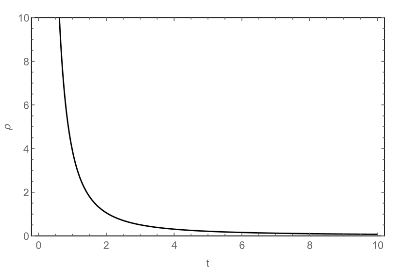
Figure 1: Energy density $\rho$ versus time $t$
($m=1.1,$ $n=0.05,$ $k=0.1,$ $l=0.9$)

Figure 2: EoS parameter $\omega$ versus time $t$
($m=1.1,$ $n=0.05,$ $k=0.1,$ $l=0.9$)

where $\chi(l)=\frac{l-1}{(l+1)^{2}}$.The plots for the energy density and EoS parameter has been shown in FIG-1 and FIG-2 respectively by choosing appropriate adjustable constants to see the time evolution of these parameters. The behaviour of the energy density would be decided by the power of the cosmic time in the expression (20). At the late cosmic phase the energy density $\rho\simeq 2\left(\frac{l^{2}+4l+1}{l^{2}+2l+1}\right)\left(nln\xi\right)^{2}$. It has been observed that both in early time and late time the energy density remain positive. It might be negative if the second term in eqn. (20) dominates the first term. However, we have already adjusted the functions in such a way that the energy density remains positive throughout the cosmic evolution. The EoS parameter starts in the negative region and stays in the acceptable range Mathew15 . Hence, it can be infer that the matter evolves in the quintessence region at early time and remains in the same domain till late phase of cosmic time and approaching towards phantom barrier. The parameter evolves dynamically with the expansion of the universe. This is basically governed by the rest energy density that appears in the denominator of eqn. (21). Moreover, it is worthy to mention here that since the exponent $n$ and the value of $\xi$ are positive, at late phase $\omega\sim-1$. Subsequently, we obtained the skewness parameters as:

$$\delta=-\left(\frac{l-1}{\rho}\right)\left(\frac{2}{3}\chi(l)\right)\left[3\left(nln\xi+\frac{m}{t}\right)^{2}-\frac{m}{t^{2}}\right]$$ (22)

$$\gamma=\left(\frac{l+5}{2\rho}\right)\left(\frac{2}{3}\chi(l)\right)\left[3\left(nln\xi+\frac{m}{t}\right)^{2}-\frac{m}{t^{2}}\right]$$ (23)

$$\eta=-\left(\frac{5l+1}{2\rho}\right)\left(\frac{2}{3}\chi(l)\right)\left[3\left(nln\xi+\frac{m}{t}\right)^{2}-\frac{m}{t^{2}}\right]$$ (24)

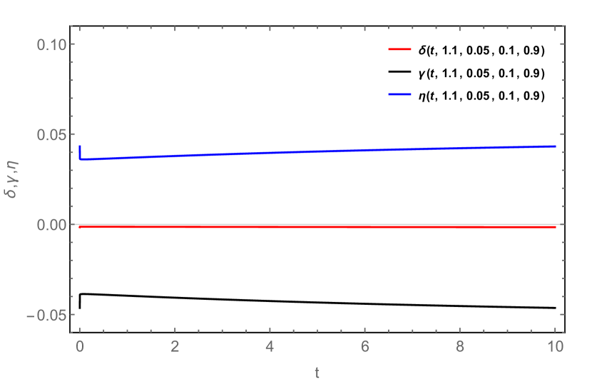
Figure 3: Skewness parameters versus time $t$
($m=1.1,$ $n=0.05,$ $k=0.1,$ $l=0.9)$

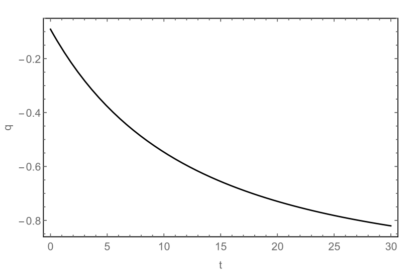
Figure 4: Deceleration parameter $q$ versus time $t$
($m=1.1,$ $n=0.05,$ $k=0.1,$ $l=0.9$)

The plot for the anisotropic parameters and cosmic time has been represented in FIG-3. The functional $\frac{f(t)}{\rho}$ is also time varying, as the energy density $\rho$ has been changing with the time. So, the evolutionary behaviour of the skewness parameters $\delta$, $\eta$ and $\gamma$ which are negative at early cosmic time and positive in the late phase have been decided by the factor $\frac{f(t)}{\rho}$. As expected, the skewness parameter along $x-$axis does not evolve with time and mostly remains close to zero. This expectation is because in our initial assumption along $x-$axis, the expansion rate is assumed to be the same as the mean Hubble rate. It also indicates that the the pressure of the anisotropic fluid also same with the mean pressure. It is also very much notable that the other skewness parameters $\gamma$ and $\eta$ are found to be the mirror image of each other. This may be due to the fact that the anisotropic parameter $l$ is close to 1, which will describe the small anisotropic nature of the universe (FIG-4). The constants (model parameters) are adjusted in such a way that the present numerical values of the cosmological parameters lie in the neighbourhood of predicted values by the observational data. In FIG-4, $q(t_{0})\sim-0.8$ where $t_{0}=13.7$ billion years. Here, 2 units of cosmic time $t$ measured as 1 billion year. So, the current assigned value for cosmic time $t_{0}$ = 28 units, gives $t_{0}\sim 13.7$ billion years.

The scalar expansion and shear scalar of the model can be obtained respectively as $\theta=3nln\xi+\frac{3m}{t}$ and $\sigma^{2}=\left(\frac{l-1}{l+1}\right)^{2}\left(nln\xi+\frac{m}{t}\right)^{2}$. These parameters confirm the rate of change of local volume of the corresponding model in an increasing way since all $m$,$n$ and $\xi$ are positive. Also, the deceleration parameter can be obtained as $q=-\frac{1}{H^{2}}\left((nln\xi)^{2}+\frac{m(m-1)}{t^{2}}+\frac{m}{t}\right)$. The deceleration parameter remains negative and time dependent for $m>1$ and $n>0$ with a negative value at early phase and $q\sim-1$ at late times of acceleration agreeing with the present observational result.

III.2 Case II

In this case, we have considered the scale factor as a hyperbolic function in the form

$$R(t)=\alpha cosh\beta t$$ (25)

where $\alpha$, $\beta$ are positive constants and the Hubble parameter obtained as $H=\beta tanh\beta t$. Subsequently the directional Hubble parameters can be obtained as: $H_{1}=H=\left(\beta tanh\beta t\right)$, $H_{2}=\left(\frac{2l}{l+1}\right)\left(\beta tanh\beta t\right)$ and $H_{3}=\left(\frac{2}{l+1}\right)\left(\beta tanh\beta t\right)$. Now, we can obtain the functional $f(H)$, for the considered Hubble parameter as

$$f(t)=\frac{2}{3}\left[\beta^{2}\left(1+2tanh^{2}\beta t\right)\right]$$ (26)

The energy density and the EoS parameter can be expressed as:

$$\rho=2\left(\frac{l^{2}+4l+1}{l^{2}+2l+1}\right)\left(\beta tanh\beta t\right)^{2}-3\left(\frac{k}{\alpha cosh\beta t}\right)^{2}$$ (27)

$$\omega=-\frac{2}{\rho}\left(\frac{l^{2}+4l+1}{l^{2}+2l+1}\right)\left[\frac{2}{3}\beta^{2}\left(1+\frac{1}{3}tanh^{2}\beta t\right)\right]+\frac{1}{\rho}\left(\frac{k}{\alpha cosh\beta t}\right)^{2}$$ (28)

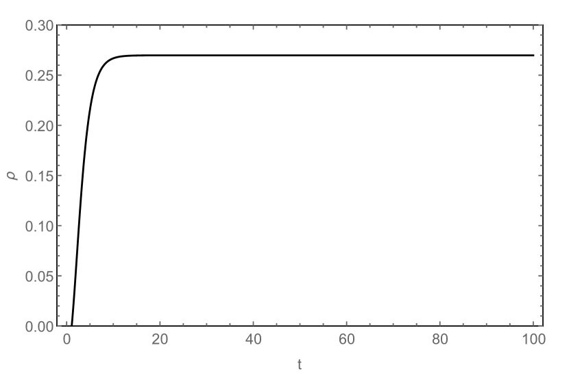
Figure 5: Energy density $\rho$ versus cosmic time $t$
($\alpha=1,$ $\beta=0.30,$ $k=0.1,$ $l=0.9)$

Figure 6: EoS parameter $\omega$ versus cosmic time $t$
($\alpha=1,$ $\beta=0.30,$ $k=0.1,$ $l=0.9)$

It has been observed that the energy density increases with increase in time and remain flat after a particular time period. Initially there is a sharp increase and subsequently the increment becomes constant at late time. The details has been shown in FIG-5. It may be noted here that since $\rho$ needs to be positive, the first term of (27), should dominates the second. Therefore the behaviours of the parameters are constrained accordingly within the admissible limit. The EoS parameter in FIG-6 shows phantom behaviour in early phase of cosmic time ($t\sim 1.7$ billion years) and evolves dynamically. However, it crosses the phantom barrier at $t=5.8$ before stabilising in the quintessence region as referred by current Planck satellite data ( $\omega=-1.49_{-0.57}^{+0.05}$ )Mathew15 ; Brevik15 . The skewness parameters of the model with this scale factor can be obtained as:

$$\delta=-\left(\frac{l-1}{\rho}\right)\left(\frac{2}{3}\chi(l)\right)\left[\beta^{2}\left(1+2tanh^{2}\beta t\right)\right]$$ (29)

$$\gamma=\left(\frac{l+5}{2\rho}\right)\left(\frac{2}{3}\chi(l)\right)\left[\beta^{2}\left(1+2tanh^{2}\beta t\right)\right]$$ (30)

$$\eta=-\left(\frac{5l+1}{2\rho}\right)\left(\frac{2}{3}\chi(l)\right)\left[\beta^{2}\left(1+2tanh^{2}\beta t\right)\right]$$ (31)

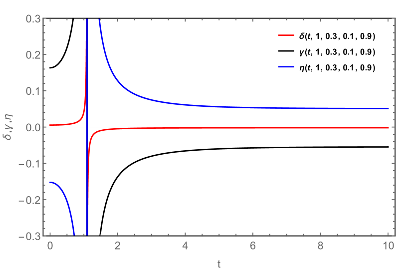
Figure 7: Skewness parameters versus time $t$
($\alpha=1,$ $\beta=0.30,$ $k=0.1,$ $l=0.9)$

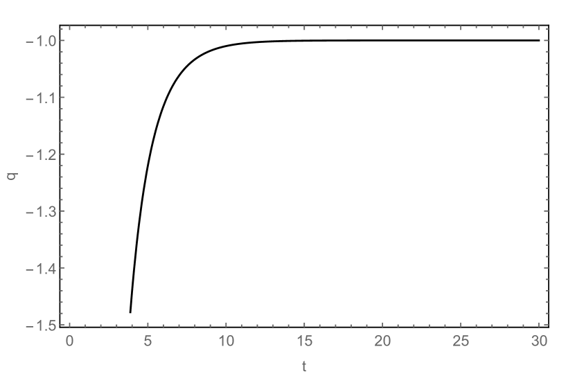
Figure 8: Deceleration parameter $q$ versus time $t$ ($\alpha=1,$ $\beta=0.30,$ $k=0.1,$ $l=0.9)$

In FIG-7, we have represented the behaviour of skewness parameters with respect to the cosmic time. As in the previous case, in this case also the skewness parameter $\delta$ does not evolve with time and move all along the x-axis with increase in $t$. In fact it lies entirely on the $x-$axis at late times. At the same time the other two skewness parameters $\gamma$ and $\eta$ remain constant at late times respectively in the positive and negative side of $x-$axis. Both these parameters maintain a uniform distance from the parameter $\delta$. The scalar expansion of the model can be calculated as $\theta=3\beta tanh\beta t$, which indicates that the expansion increases with increase in time. The shear scalar found to be $\sigma^{2}=\left(\frac{l-1}{l+1}\right)^{2}\beta^{2}tanh^{2}\beta t$. Irrespective of the value of the aniostropic value $l$, the shear scalar is positive through out the evolution. Both the shear scalar and scalar expansion indicate that the rate of deformation is positive with respect to the cosmic evolution through the transition. Scalar expansion remains positive for positive value of $\beta$ whereas in shear scalar $l$ need to constraint as $l>1$ in order to get a positive cosmic behaviour. The deceleration parameter is found to be $q=-tanh^{2}\beta t$, it indicates that the parameter always remain negative and close to $-1$ for $\beta=0.30$, adhere to a good match with the observational data. It is also observed from FIG-8 that the accelerated expansion occur in a reasonable time period, which can be termed as the transition period.

III.3 Case III

In the previous two cases, we have constructed the dark energy models by considering the scale factor as a hybrid and hyperbolic functions. In order to have a better understanding on the anisotropic universe, in this case, we have considered the scale factor as a fraction of exponential function in the form:

$$H(R)=a(R^{-n}+1)=\frac{ae^{nat}}{e^{nat}-1}$$ (32)

where $a$, $b$ are positive constants. The scale factor $R$ can be expressed as $R=(e^{nat}-1)^{\frac{1}{n}}$. Now, we can obtain the functional $f(H)$ as

$$f(t)=\frac{2}{3}\left[-na^{2}e^{nat}+\frac{3a^{2}e^{2nat}}{(e^{nat}-1)^{2}}\right]$$ (33)

The energy density and EoS parameter can be obtained as,

$$\rho=2\left(\frac{l^{2}+4l+1}{l^{2}+2l+1}\right)\left(\frac{ae^{nat}}{e^{nat}-1}\right)^{2}-3\left(\frac{k}{(e^{nat}-1)^{\frac{1}{n}}}\right)^{2}$$ (34)

$$\omega=-\frac{2}{\rho}\left(\frac{l^{2}+4l+1}{l^{2}+2l+1}\right)\left[-\frac{2na^{2}e^{nat}}{3}+\left(\frac{ae^{nat}}{e^{nat}-1}\right)^{2}\right]+\frac{1}{\rho}\left(\frac{k}{\left(e^{nat}-1\right)^{\frac{1}{n}}}\right)^{2}$$ (35)

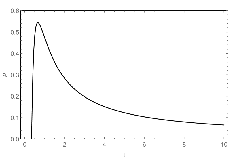
Figure 9: Energy density $\rho$ versus time $t$
($n=0.99,$ $a=0.1,$ $k=0.1,$ $l=0.9)$

Figure 10: EoS parameter $\omega$ versus time $t$
($n=0.99,$ $a=0.1,$ $k=0.1,$ $l=0.9)$

The energy density in FIG-9 lies in the positive domain. Though initially, it rises sharply but at late times it decreases rapidly. The most common type of dark energy is the EoS parameter with the ratio of pressure and dark energy density is a constant. Such an EoS is well known if $\omega\in[0,1]$, which describes a perfect fluid; however with $\omega=-1$, it defines a cosmological constant. When $\omega<-\frac{1}{3}$, the universe is filled with some similar substance which leads to the expansion with acceleration. However, in most of the cases it remains in the range $({-\frac{1}{3},-1})$. From FIG-10, it is observed that, $\omega$ evolves in the phantom era at early cosmic time and slides through the quintessence region at late time, crossing the phantom barrier at $t=5.75$ billion years. The parameter proceeds towards still higher values in later evolution and remains in the preferred observed range. The skewness parameters for the model can be obtained as:

$$\delta=-\left(\frac{l-1}{\rho}\right)\left(\frac{2}{3}\chi(l)\right)\left[-na^{2}e^{nat}+\frac{3a^{2}e^{2nat}}{(e^{nat}-1)^{2}}\right]$$ (36)

$$\gamma=\left(\frac{l+5}{2\rho}\right)\left(\frac{2}{3}\chi(l)\right)\left[-na^{2}e^{nat}+\frac{3a^{2}e^{2nat}}{(e^{nat}-1)^{2}}\right]$$ (37)

$$\eta=-\left(\frac{5l+1}{2\rho}\right)\left(\frac{2}{3}\chi(l)\right)\left[-na^{2}e^{nat}+\frac{3a^{2}e^{2nat}}{(e^{nat}-1)^{2}}\right]$$ (38)

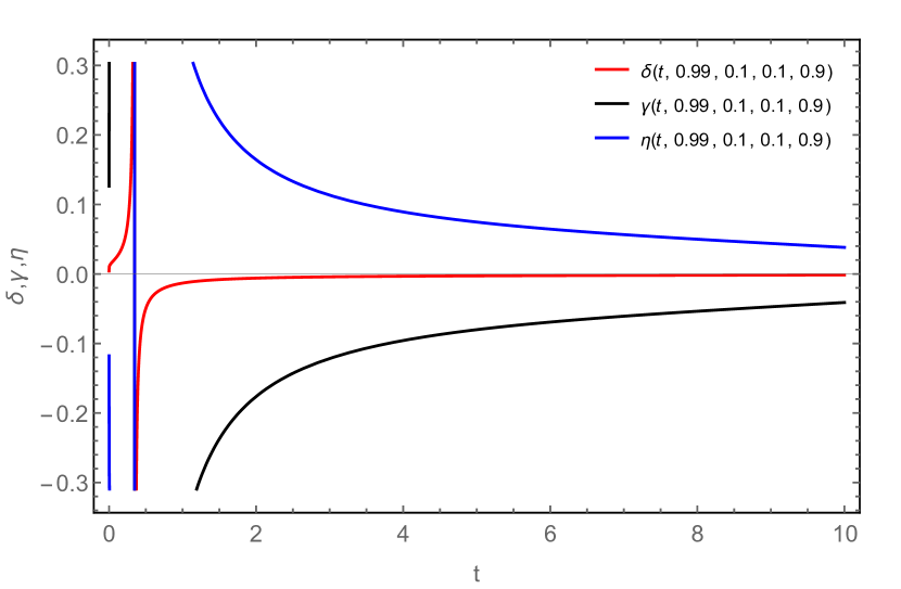
Figure 11: Skewness parameters versus time $t$
( $n=0.99,$ $a=0.1,$ $k=0.1,$ $l=0.9)$

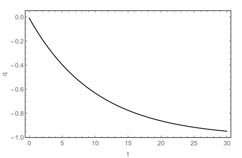
Figure 12: Deceleration parameter $q$ versus time $t$
( $n=0.99,$ $a=0.1,$ $k=0.1,$ $l=0.9)$

FIG-11 describes the behaviour of the skewness parameters of the model. Here also the parameter $\delta$ aligned with the $x-$axis and $\gamma$, $\eta$ remain as the mirror image of each other. In this case, the scalar expansion and shear scalar can be obtained respectively as $\theta=\frac{3ae^{nat}}{e^{nat}-1}$ and $\sigma^{2}=\left(\frac{l-1}{l+1}\right)^{2}\left(\frac{ae^{nat}}{e^{nat}-1}\right)^{2}$. Scalar expansion shows the change of volume of the corresponding universe in an accelerated way as it includes exponential terms. Similarly shear scalar indicated the deformation rate of the universe is positive always for $l>1$ and $a>0$. The deceleration parameter $q=-\frac{n}{e^{nat}(e^{nat}-1)}-(1-n)$. The behaviour of deceleration parameter in FIG-12 indicates the acceleration expansion at late time; however at early time it might have decelerated. In order to get an accelerated expansion of the universe $n<1$. It can be noted that $q(t_{0})\sim-0.7$ when $t_{0}=13.7$ billion years.

IV Conclusion

We have considered three different functional forms of scale factor to construct some DE cosmological models of the Universe in the framework of GR. The space time at the backdrop considered is the spatially homogeneous anisotropic Bianchi V metric. With the help of the forms of scale factor and Hubble expansion rates along different directions, the anisotropic behaviour of the dark energy driven cosmological model has been simulated. In the first and third case, we have observed that at late phase of cosmic dynamics, the accelerated expansion of the universe has occurred; however before this the universe might have decelerating at early time whereas in the second case it reveals the time period of cosmic transition from early deceleration phase to late time acceleration phase. The EoS parameters in case I and III become time varying. In case I, where the scale factor is in the form of general hybrid factor, the EoS parameters entirely remain in the quintessence region. However in case II, it starts evolving from phantom phase and in case III it evolves from phantom dominated era but approaches towards false vacuum model, lying primarily in the quintessence region.

The skewness parameters in case I and II indicates pressure anisotropy of late phase evolving dynamically with cosmic expansion. In all the cases skewness parameters evolve fluctuating from different ranges showing greater anisotropy. In case III, the parameters continue their behaviour towards an isotropic universe but in the other two cases pressure anirotropy remains constant. In the present work, we observed that, the constant in the functional form of the scale factors in (17) is used to reconstruct different DE anisotropic models, depending on Hubble parameter, we revealed more interesting results favouring phantom kind of behaviour and quintessence dominated era. It is concluded that pressure anisotropic in DE fluid play very important and interesting role of pressure anisotropic need to be carried out for further better understanding of the accelerated expansion of the universe.

V References

E. J. Copeland, M. Sami, S. Tsujikawa, Int. J. of Mod. Phys., D15 (2006) 1753.

B. Wang, E. Abdalla, F. Atrio-Barandela, D. Pavon, Rep. Prog. Phys.,  79(9) (2016) 096901.

P.A.R. Ade et al., Planck Collaboration, Astron. Astrophys., 571 (2014) A16.

M.Watanabe, S.Kanno, J. Soda, Phys. Rev. Lett., 102 (2009) 191302.

R. Buiny, A. Berera, T. W. Kephart, Phys. Rev., D73 (2006) 063529.

S. K. Tripathy, Astrophys. Space Sci., 350(2014) 367.

C. Armendariz-Picon, J. Cosmol. Astro. Phys., 0407 (2004) 007.

T. R. Jaffe, A. J. Banday, H. K. Eriksen, K. M. Gorski, F. K. Hansen, Astrophys. J., 629 (2005) L1.

T. Koivisto and D. F. Mota, J. Cosmol. Astro. Phys., 0806 (2008) 018.

A. Cooray, D. E. R. Caldwell, J. Cosmol. Astro. Phys., 1011 (2010) 015.

R. Cook, D. Lynden-Bell, Mon. Not. R. Astron. Soc., 401 (2010) 1409.

L. Campanelli, P. Cea, L. Tedesco, Phys. Rev. Lett., 97 (2006) 131302 .

L. Campanelli, Phys. Rev., D80 (2009) 63006.

A. Gruppo, Phys. Rev., D76 (2007) 83010.

T. Koivisto, D. F. Mota, Phys. Rev., D73 (2006)083502.

T. Koivisto, D. F. Mota, Astrophysical Journal, 679 (2008)1.

R. Battye, A. Moss, Phys. Rev., D80 (2009)023531.

O. Akarsu and C. B. Kilinc, Gen. Relativ. Gravit., 42 (2010) 119.

O. Akarsu and C. B. Kilinc, Gen. Relativ. Gravit., 42 (2010) 763.

B. Mishra, P. K. Sahoo and S. K. Tripathy, Astrophys. Space Sci., 356 (2015) 163.

B. Mishra, S. K. Tripathy, Mod. Phys. Lett. A, 30(2015) 1550175.

S. K. Tripathy, B. Mishra and P.K. Sahoo, arXiv:1503.05109v1 [gr-qc].

O. Akarsu, S. Kumar, R. Myrzakulov, M. Sami, L. Xu, J. Cosmol. Astropart. Phys., 01, (2014) 22.

S.K.J. Pacif, R. Myrzakulov, S. Myrzakul, arXiv: 1609.02801v1 [gr-qc], (2016).

B.Mishra, P.K. Sahoo, Pratik P. Ray, Int. J. Geom. Method. Mod. Phys., 14, (2017) 1750124.

B.Mishra, S.K.Tripathy, Pratik P. Ray, arXiv:1701.08632v1 [physics.gen-ph],(2017).

T.K. Mathew, C. Murli, J. Shejeelammal, arXiv:1506.02123v3 [gr-qc], (2015).

I. Brevik, Entropy, 17 (2015) 6318.