Single-particle dispersion in stably stratified turbulence

Abstract

We present models for single-particle dispersion in vertical and horizontal directions of stably stratified flows. The model in the vertical direction is based on the observed Lagrangian spectrum of the vertical velocity, while the model in the horizontal direction is a combination of a continuous-time eddy-constrained random walk process with a contribution to transport from horizontal winds. Transport at times larger than the Lagrangian turnover time is not universal and dependent on these winds. The models yield results in good agreement with direct numerical simulations of stratified turbulence, for which single-particle dispersion differs from the well studied case of homogeneous and isotropic turbulence.

I Introduction

Lagrangian statistics in fluid dynamics offer unique insight into particle dispersion (e.g., dispersion of pollutants and transport of nutrients in the ocean) and turbulent mixing Yeung (2002); Toschi and Bodenschatz (2009); Zimmermann et al. (2010); Falkovich et al. (2012); Pumir et al. (2016); Bec et al. (2006); Thalabard et al. (2014). Often such transport occurs in settings such as the atmosphere and oceans, in which turbulence is either inhomogeneous or non-isotropic due to stratification or rotation Wyngaard (1992); Biferale et al. (2016). While particle dispersion in homogeneous and isotropic turbulence (HIT) has received significant attention, particle dispersion in anisotropic flows such as stably stratified turbulence has been studied only recently both in the presence of rotation Liechtenstein et al. (2005, 2006) and without Kimura and Herring (1996); Aartrijk et al. (2008); Sozza et al. (2016). Under stable stratification vertical dispersion is known to be suppressed Kaneda and Ishida (2000), but its effect on horizontal transport is less certain Liechtenstein et al. (2006); Aartrijk et al. (2008).

The study of the role of anisotropies in turbulent mixing is of central importance in fluid dynamics, as well as in many geophysical applications. By now it is clear that the presence of restoring forces such as gravity or rotation, and of their associated waves, can have a profound impact in the properties of a turbulent flow which cannot be treated as small corrections to HIT Sagaut and Cambon (2008). In the particular case of stratified turbulence, which plays a key role in geophysics, linear and non-linear processes (such as the zig-zag instability Billant and Chomaz (2001), or non-linear resonant interactions of internal gravity waves Smith and Waleffe (2002)) result in a preferential transfer of energy towards vortical modes, associated with the development of pancake-like structures (i.e., of structures in the flow with typical horizontal scales much larger than typical vertical scales), and of strong horizontal winds with vertical shear Marino et al. (2014); Clark di Leoni and Mininni (2015). Horizontal turbulent transport in this case can thus be expected to share similarities with other sheared flows, such as sheared flows in neutral fluids and in plasmas Terry (2000). Moreover, the understanding of turbulent transport and mixing in the particular case of stably stratified turbulence is crucial for atmospheric sciences and oceanography. In the tropopause, three-dimensional mixing is believed to play a crucial role in the exchange of chemical compounds between the stratosphere and the troposphere Shapiro (1980). In the oceans, how three-dimensional mixing develops is important to understand the observed density of phytoplankton Davis and Yan (2004), with implications for the management of halieutic resources and the fishing industry.

Here we study single-particle statistics in forced stably stratified turbulence using direct numerical simulations. We show that for frequencies smaller than the buoyancy frequency, the Lagrangian vertical velocity follows a spectrum similar to others observed in wave-dominated flows in the ocean D’Asaro and Lien (2000), and which are often described by an empirical Garrett-Munk (GM) spectrum Garrett and Munk (1975); Lien et al. (1998). We then present models for both vertical and horizontal dispersion. The former (transport parallel to the mean stratification) indicates that the reason for the reduced dispersion in this direction is that the flow is dominated by a random superposition of internal gravity waves. In the latter (transport perpendicular to the stratification), dispersion differs from HIT as it is strongly influenced by the large scale shearing flow generated by the stratification, and which plays an important role in the atmosphere Smith and Waleffe (2002); Marino et al. (2014); Clark di Leoni and Mininni (2015). The model used in this case is then a continuous-time eddy-constrained (CTEC) random walk (which accounts for particle trapping observed in HIT Rast et al. (2016)), with a superposed drift caused by the vertically sheared horizontal winds (VSHW) in stably stratified turbulence.

The implications of the models are twofold. On one hand, they provide a tool to understand fundamental processes affecting turbulent transport in stratified flows. On the other hand, as the models have no free parameters and their only ingredients are obtained from Lagrangian properties of the turbulence or from a knowledge of the large-scale flow (which in atmospheric and oceanic flows can be obtained to a good degree by large-scale models), they provide a statistical way to predict moments of the probability density function (PDF) of single-particle dispersion without requiring an ensemble of runs with explicit integration of a large number of tracers. In the next section we describe the numerical simulations, while in Sec. III we present the numerical results for vertical and horizontal dispersion and introduce the models. Finally, we present our conclusions in Sec. IV.

II The Boussinesq equations

For the numerical simulations we solved the Boussinesq equations for the velocity ${\bf u}$ and as well as for “temperature” fluctuations $\theta$ (written in units of velocity),

$$\frac{\partial{\bf u}}{\partial t}+{\bf u}\cdot{\bf\nabla}{\bf u} = -{\bf\nabla}p+N\theta{\hat{z}}+\nu\nabla^{2}{\bf u}+{\bf f},$$ (1)

$$\frac{\partial\theta}{\partial t}+{\bf u}\cdot{\bf\nabla}\theta = -N{\bf u}\cdot{\hat{z}}+\kappa\nabla^{2}\theta,$$ (2)

with the incompressibility condition ${\bf\nabla}\cdot{\bf u}=0$. Here $p$ is the pressure, $\nu$ the kinematic viscosity, ${\bf f}$ an external mechanical forcing, $N$ the Brunt-Väisälä frequency (which sets the background stratification), and $\kappa$ the thermal diffusivity. The equations were solved in a three-dimensional periodic domain of dimensionless linear length $2\pi$, using a parallel dealiased pseudospectral method and a second-order Runge-Kutta scheme for time integration Mininni et al. (2011). All runs have a spatial resolution of $512^{3}$ regularly spaced grid points, and $\nu=\kappa=8\times 10^{-4}$ in dimensionless units (thus, the Schmidt number is $\textrm{Sc}=\nu/\kappa=1$). In all runs described below, once the systems reached a turbulent steady state, we injected $10^{5}$ Lagrangian particles distributed randomly in the box. We used a high order method to integrate the equations for the Lagrangian particles

$$\frac{d{\bf x}_{i}}{dt}={\bf u}({\bf x}_{i},t),$$ (3)

(where the subindex $i$ corresponds to the particle label), using a second-order Runge-Kutta method in time, and three-dimensional third-order spline interpolation to estimate the Lagrangian velocity at points that do not correspond to grid points of the fluid code (see, e.g., Yeung and Pope (1988)). Particles move in the periodic domain, and thus we assume homogeneity of the turbulent flow to re-enter particles that escape out of the domain using periodicity.

The flows were forced at $k=1$ and $2$ with two different mechanical forcings. A set of two simulations (with different Brunt-Väisälä frequencies, $N=4$ or $N=8$) was forced with Taylor-Green (TG) forcing Clark di Leoni and Mininni (2015), which is a two-component forcing which generates pairs of counter-rotating von Kármán swirling flows in planes perpendicular to the stratification, and with a shear layer in between them. When applied at only one wavenumber ($k=k_{f}$, the forcing wavenumber), TG forcing is given by

$${\bf f_{TG}}(k_{f})=f_{0}\left(sin(k_{f}x)cos(k_{f}y)cos(k_{f}z),-cos(k_{f}x)sin(k_{f}y)cos(k_{f}z),0\right).$$ (4)

For $k_{f}=1$, this forcing has two shear layers, one at $z=\pi/2$ and another one at $z=3\pi/2$ (where ${\bf f_{TG}}=0$). Our TG forcing, applied at $k=1$ and $2$, is simply the superposition ${\bf f}={\bf f_{TG}}(1)+{\bf f_{TG}}(2)$. In the presence of stratification, this mechanical forcing generates a coherent flow at the large scales, which develops horizontal winds (i.e., a non-zero mean horizontal velocity) only in the shear layers between the von Kármán swirling flows, as the large-scale von Kármán structures prevent the formation of strong horizontal winds in the rest of the domain. Taylor-Green flows, as they excite directly only horizontal components of the velocity, have been used before to study stratified flows and geophysical turbulence Riley and de Bruyn Kops (2003).

Another set of two simulations (also with Brunt-Väisälä frequencies $N=4$ or $8$) was forced using isotropic three-dimensional random forcing (RND) with a correlation time of half a large-scale turnover time. Every $\Delta t=0.5$, a forcing with random phases $\phi_{\bf k}$ for each Fourier mode ${\bf k}$ in the shell $k\in[1,2]$ was generated as

$${\bf f_{1}}=f_{0}\sum_{|{\bf k}|\in[1,2]}\Re\left[i{\bf k}\times{\bf\hat{r}}e^{i({\bf k}\cdot{\bf\hat{r}}+\phi_{\bf k})}\right],$$ (5)

where $\Re$ stands for the real part. The forcing ${\bf f}$ is obtained by slowly interpolating the forcing from a previous random state ${\bf f_{0}}$ to the new random state ${\bf f_{1}}$, in such a way that ${\bf f}={\bf f_{1}}$ after $\Delta t$. The process is then repeated to obtain a slowly evolving random forcing which does not introduce spurious fast time scales in the evolution of the Lagrangian particles. With this forcing, no large-scale coherent flows are sustained, and horizontal winds can then grow in the entire domain. Also, as this forcing is isotropic, a larger amount of injected power will go into excitation of internal gravity waves, as confirmed below. Thus, the large scales of both sets of simulations have very different behaviors. In the Appendix we discuss a third forcing function, to further validate the model for horizontal dispersion discussed in the next section using yet another configuration.

Equations (1) and (2) have two control dimensionless parameters. The Reynolds number

$$\textrm{Re}=\frac{LU}{\nu},$$ (6)

where $L$ and $U$ are respectively the characteristic Eulerian length scale and velocity of the flow, and the Froude number

$$\textrm{Fr}=\frac{U}{LN},$$ (7)

which measures the ratio of inertial forces to buoyancy forces in Eq. (1). The characteristic velocity $U$ is estimated as the root mean square Eulerian velocity. From the Reynolds and Froude numbers, we can also define the buoyancy Reynolds number,

$$\textrm{Re}_{b}=\textrm{Re}\,\textrm{Fr}^{2},$$ (8)

which gives a measure of the strength of the turbulence in the stratified flow, and is associated with the turbulent mixing as well as with the relevance of viscous effects at all scales in these flows (see, e.g., Ivey et al. (2008)).

Another useful parameter to estimate the turbulent mixing is the local gradient Richardson number (see, e.g., Rosenberg et al. (2015))

$$Ri_{g}=\dfrac{N(N-\partial_{z}\theta)}{\partial_{z}(u_{\perp}^{2})},$$ (9)

where $u_{\perp}=(u_{x}^{2}+u_{y}^{2})^{1/2}$. Note that this is a pointwise expression. Values of $Ri_{g}<1/4$ can be considered to be an indication of possible local shear instabilities at that point, while for $Ri_{g}<0$ local overturning can occur.

In the previous expressions and in the following, the characteristic Eulerian length scales (or the integral scales) for all runs are computed from the Eulerian kinetic energy spectrum $E(k)$ of these flows as

$$L=2\pi\dfrac{\int{E(k)k^{-1}dk}}{\int{E(k)}dk},$$ (10)

$$L_{\parallel}=2\pi\dfrac{\int{E(k_{\parallel})k_{\parallel}^{-1}dk_{\parallel}}}{\int{E(k)}dk},$$ (11)

and

$$L_{\perp}=2\pi\dfrac{\int{E(k_{\perp})k_{\perp}^{-1}dk}}{\int{E(k)}dk},$$ (12)

where $L$ is the isotropic Eulerian length scale, $L_{\parallel}$ is the parallel or vertical Eulerian length scale, and $L_{\perp}$ is the perpendicular or horizontal Eulerian length scale.

Finally, two other relevant parameters for the next section are the Eulerian correlation time (or the large-scale turnover time), given by $T_{e}=L/U$, and the Lagrangian turnover time $T_{l}$, which is the mean correlation time of single-particle trajectories. Table 1 gives the values of the parameters and characteristic scales introduced in this section for all runs.

Run	Forcing	$N$	$\nu$	Re	Fr	$\textrm{Re}_{b}$	$T_{e}$	$T_{l}$	$L$	$L/L_{\parallel}$	$L/L_{\perp}$
TG4	TG	$4$	$8\times 10^{-4}$	7000	$0.04$	11	$3.6$	$7.2$	$2.2$	$0.9$	$0.5$
TG8	TG	$8$	$8\times 10^{-4}$	7000	$0.02$	3	$2.9$	$8.0$	$2.8$	$1.0$	$0.5$
RND4	RND	$4$	$8\times 10^{-4}$	13000	$0.08$	83	$2.0$	$25.5$	$3.5$	$1.1$	$0.8$
RND8	RND	$8$	$8\times 10^{-4}$	13000	$0.04$	21	$2.5$	$17.1$	$3.6$	$1.1$	$0.6$

Table 1: Parameters and Eulerian and Lagrangian characteristic scales for all runs: TG and RND stand respectively for Taylor-Green and random isotropic forcing, $N$ is the Brunt-Väisälä frequency, $\nu$ is the kinematic viscosity ($\kappa=\nu$), Re is the Reynolds number, Fr is the Froude number, $\textrm{Re}_{b}$ is the buoyancy Reynolds number, $T_{e}$ and $T_{l}$ are respectively the characteristic Eulerian and Lagrangian time scales, $L$ is the isotropic Eulerian integral length scale, and $L/L_{\parallel}$ and $L/L_{\perp}$ are the ratios of this scale respectively to the parallel and to the perpendicular integral length scales.

III Results

III.1 Particle trajectories

Figure 1 shows vertical and horizontal displacements for a few particles in the RND4 simulation (random forcing with $N=4$; in the following we label runs by their forcing followed by the value of $N$, following the notation in table 1), and in the TG4 simulation (i.e., Taylor-Green forcing with $N=4$). In both simulations, while vertical displacements are small and display wave-like motions, horizontal motions are large (compared with the periodic domain size of $2\pi$). In the RND4 simulation horizontal trajectories seem almost ballistic at all times, being dominated by a strong drift. Note also that particles at different heights (indicated by the different colors) move in different directions, as the horizontal winds in each layer also point in different directions. In the TG4 simulation, horizontal displacements show only a fraction of the particles with such a drift (those in the vicinity of the horizontal layers where Taylor-Green forcing is zero, and all moving along the same direction), and a significantly stronger trapping of particles by eddies which can be seen as particle trajectories turn around.

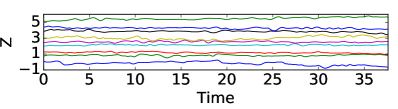
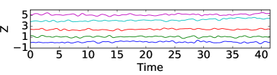
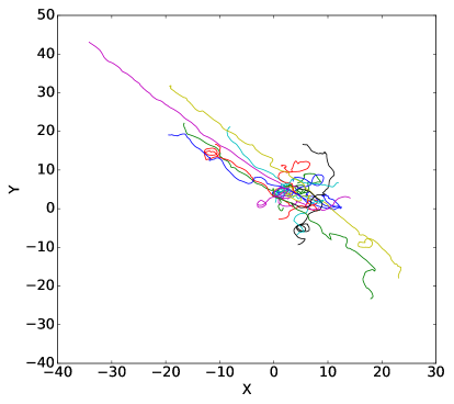
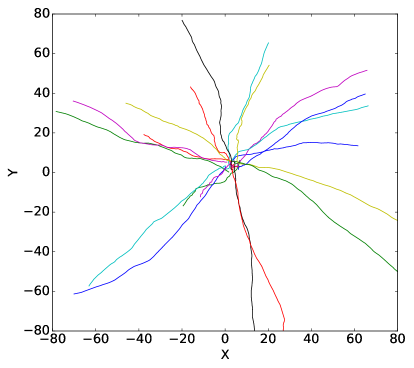
Figure 1: (Color online) Left column: Vertical (top) and horizontal (bottom) displacements for a few particles (indicated by different colors) in the TG4 run (Taylor-Green forcing with $N=4$). Right column: Same for the RND4 run (random forcing with $N=4$).

III.2 Lagrangian spectra

The Lagrangian spectrum of the vertical velocity is shown in Fig. 2. The spectra of all simulations are shallow for frequencies $\omega/N<1$, and show a peak near $\omega/N=1$, i.e., the parallel kinetic energy is concentrated near the buoyancy frequency. The shallow spectra for frequencies $\omega/N<1$ are reminiscent of the GM spectrum, which is an empirical spectrum for internal oceanic waves Garrett and Munk (1975); Lien et al. (1998); D’Asaro and Lien (2000) that reflects the dominance of wave contributions. The spectrum was first derived for the total energy, but later generalized for vertical velocities Garrett and Munk (1975), and used to compare with Lagrangian measurements (see, e.g., D’Asaro and Lien (2000); D’Asaro et al. (2007)). In the absence of rotation, i.e., at oceanic scales much smaller than the scales at which rotation is relevant, the spectrum reduces to a white spectrum for $\omega\leq N$. For frequencies $\omega/N>1$ the vertical Lagrangian spectra in Fig. 2 decrease rapidly (in some cases following a power law). Only as a reference, in Fig. 2 (left) we show two power laws, for frequencies $\omega/N\lesssim 1$, and for $\omega/N>1$.

On this light, we can interpret the observed vertical Lagrangian spectrum as follows. For frequencies $\omega/N<1$, the shallow spectrum corresponds to a superposition of internal gravity waves and is dominated by their contributions. Indeed, as the dispersion relation of internal gravity waves is $\omega=Nk_{\perp}/k\leq N$, waves can only contribute to frequencies with $\omega/N\leq 1$. For $\omega/N>1$ waves cannot contribute, and any power at those frequencies must come from fast vortical motions and turbulence, as also observed in oceanic measurements where power laws were also reported for frequencies larger than the buoyancy frequency D’Asaro and Lien (2000). Moreover, note that the RND simulations have steeper spectra at frequencies larger than the Brunt-Väisälä frequency, even though they have larger Fr and $\textrm{Re}_{b}$ numbers. This is compatible with a stronger predominance of waves in those runs, associated with the direct excitation of waves by the isotropic three-dimensional forcing. The stronger waves and the weaker turbulence in these runs will be confirmed later when we study the gradient Richardson number and we show that the TG simulations have larger probabilities of satisfying the conditions for local shear instabilities or overturning.

In all cases, the predominance of waves in the vertical Lagrangian spectra, which concentrate most of the power, is compatible with the vertical Lagrangian trajectories observed in Fig. 1: there is little dispersion in this direction, and particle displacements are dominated by wave-like motions. In comparison, Lagrangian spectra of the horizontal velocity (see Fig. 2) do not display a peak at the buoyancy frequency nor a shallow spectrum for frequencies $\omega/N<1$, although in some simulations the horizontal spectra display a knee and a change in the spectral slope in the vicinity of this frequency (especially, again, for RND forcing).

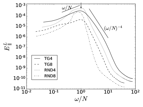
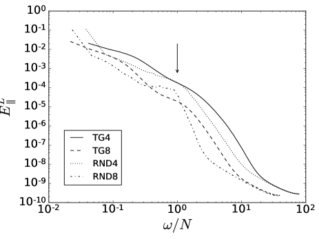
Figure 2: (Color online) Left: Lagrangian power spectrum of the vertical velocity in all simulations. Power laws are indicated as a reference (see Table 2). All spectra display a peak at the Brunt-Väisälä frequency (indicated by the arrow), and for frequencies $\omega/N<1$ the shallow spectra are reminiscent of observations of oceanic internal gravity waves. Right: Lagrangian power spectrum of the horizontal velocity. In the horizontal case there is no clear peak near the Brunt-Väisälä frequency.

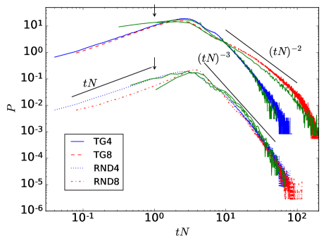
Figure 3: (Color online) PDF of vertical displacement waiting times for the simulations, and waiting times generated by the model consisting of a superposition of random waves (solid green in all cases). For TG runs the PDFs have been shifted vertically for better visualization. Power laws are shown as a reference (see Table 2), and vertical arrows indicate $t=1/N$.

III.3 Vertical dispersion

To model the small displacements in the vertical direction, we consider the statistics of vertical displacement waiting times of the Lagrangian particles. To this end, we take the waiting time as the time interval between two consecutive crossings of each particle trajectory through its mean $z$ elevation. We plot the waiting time distribution for all runs in Fig. 3. The PDFs are non-exponential, indicating the system has memory (waves carry information of their initial conditions for a finite amount of time), and are compatible with a power law for $tN\gtrsim 1$. The slope is steeper for the RND runs, $\sim t^{-3}$, than for those with TG forcing, $\sim t^{-2}$ (the best fit to these exponents, $\beta_{-}$, corresponding to the exponents for $tN>1$, as well as for exponents $\beta_{+}$ corresponding to power laws approximated for $tN<1$, are shown in table 2). Surprisingly, in the TG case, the probability of long waiting times (i.e., of large excursions of some particles from their mean $z$ position) also increases with increasing stratification. This reflects the underlying nature of the stratified turbulence, in which waves can be nonlinearly amplified Rorai et al. (2014) (note long excursions can be generated by strong low frequency waves, as observed in Fig. 2 and in the model shown next), which can also result in a local instability or in overturning. To confirm this, Fig. 4 shows the PDFs of the local gradient Richardson number $Ri_{g}$ for all runs. When $Ri_{g}<1/4$ local shear instabilities can develop, while for $Ri_{g}<0$ overturning is possible as the vertical gradient of temperature fluctuations $\partial_{z}\theta$ overcomes the background gradient associated with $N$. The TG runs have larger probability of having points with $Ri_{g}<1/4$ or $Ri_{g}<0$ when compared with the RND runs at fixed Brunt-Väisälä frequency. Also, as stratification (or equivalently, $N$) is increased, the PDFs are shifted to the right, resulting in lower probability of local shear instabilities or overturning. However, note this effect is stronger in the RND runs when compared with the TG runs. In particular, for the TG8 run there is still a considerable $(2.8\pm 0.1)\%$ probability of finding points with $Ri_{g}<0$, while for the RND8 run the probability is $(0.2\pm 0.1)\%$. This is compatible with the observations made before about the stronger prevalence of waves in the RND runs (which have larger values of $\textrm{Re}_{b}$, but are forced isotropically) when studying the Lagrangian spectrum of the vertical velocity.

Based on these observations, we thus propose a simple model for the vertical particle motion, using a superposition of waves with random phases, and with amplitudes determined by the observed parallel Lagrangian velocity $v_{\parallel}^{L}$ or by its Lagrangian spectrum $E_{\parallel}^{L}(\omega)$ on dimensional grounds as

$$A(\omega)\sim v_{\parallel}^{L}(\omega)/\omega\sim\left.\sqrt{\omega\,E_{\parallel}^{L}(\omega)}\right/\omega\sim\omega^{(\alpha_{\pm}-1)/2}.$$ (13)

Note $E_{\parallel}^{L}(\omega)$ is approximated by two power laws: one for $\omega\lesssim N$ (with exponent $\alpha_{+}>0$, see Fig. 2), and one for $\omega>N$ (with exponent $\alpha_{-}<0$). The values of the exponents $\alpha_{\pm}$ obtained from a best fit to the Lagrangian vertical spectra in Fig. 2 are shown in Table 2. The waiting times generated by this random superposition of waves are also shown in Fig. 3. The good agreement between the model and the data indicates that, at least for the Froude and Reynolds numbers considered here, the quenching of vertical dispersion results from the dominance of waves, and that the empirical knowledge of the turbulent vertical Lagrangian spectrum is sufficient to predict the probability of vertical excursions by the Lagrangian particles (at least for times comparable to several periods of the waves).

Run	$\alpha_{+}$	$\alpha_{-}$	$\beta_{+}$	$\beta_{-}$
TG4	$0.8\pm 0.3$	$-4.1\pm 0.1$	$0.8\pm 0.1$	$-2.9\pm 0.1$
TG8	$0.8\pm 0.2$	$-5.5\pm 0.1$	$0.9\pm 0.1$	$-2.0\pm 0.1$
RND4	$1.3\pm 0.4$	$-5.3\pm 0.1$	$0.9\pm 0.1$	$-3.3\pm 0.1$
RND8	$1.0\pm 0.2$	$-9.0\pm 0.1$	$1.0\pm 0.1$	$-3.3\pm 0.1$

Table 2: Exponents of power laws in the Lagrangian parallel spectrum and in the waiting time distributions for all runs, with error bars. $\alpha_{\pm}$ are the exponents of power laws obtained from a best fit to the Lagrangian parallel spectra in Fig. 2, with $\alpha_{+}$ corresponding to the exponents for $\omega/N\lesssim 1$, and $\alpha_{-}$ to the exponents approximated for $\omega/N>1$. $\beta_{\pm}$ are the exponents of power laws approximated for the waiting time distributions in Fig. 3, with $\beta_{+}$ corresponding to the exponents for $tN<1$, and $\beta_{-}$ to the exponents for $tN>1$.

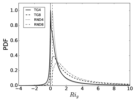
Figure 4: PDFs of the local gradient Richardson number $Ri_{g}$ for all runs. A vertical solid line at $Ri_{g}=0$ and a vertical dashed line at $Ri_{g}=1/4$ are shown as references; for $Ri_{g}<1/4$ local shear instabilities can develop, while for $Ri_{g}<0$ overturning can occur.

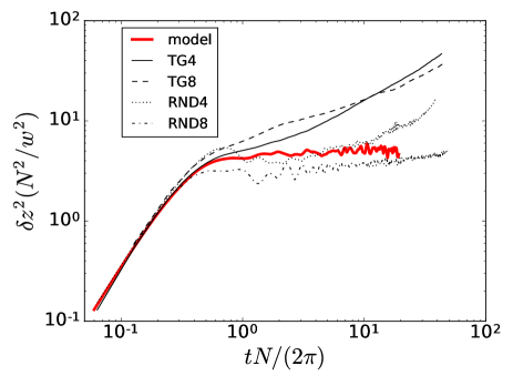
Figure 5: (Color online) Mean vertical quadratic dispersion $\delta z^{2}$ for all runs, normalized by the ratio $w^{2}/N^{2}$ of the mean squared vertical Lagrangian velocity to the squared Brunt-Väisälä frequency. Time is normalized by the Brunt-Väisälä period. All simulations collapse at early times, but the TG runs depart after $tN/2\pi\approx 1$. The thick (red) curve shows the model for RND4, which is in good agreement with the simulation until at late times molecular diffusion results in a slow vertical dispersion of the particles.

In Aartrijk et al. (2008), a normalization of the mean vertical quadratic displacement of the particles $\delta z^{2}$ was proposed to reobtain (at least for early times) a behavior similar to that found in HIT. In Fig. 5 we show $\delta z^{2}$ normalized in this way, namely by multiplying the vertical quadratic dispersion by the ratio $N^{2}/w^{2}$ of the squared Brunt-Väisälä frequency to the mean squared vertical Lagrangian velocity (with $w^{2}=\langle(v_{\parallel}^{L})^{2}\rangle$), and by multiplying time by $N/2\pi$. The quadratic vertical dispersions of all runs collapse to a single curve for $tN/2\pi\lesssim 1$, confirming the scaling proposed in Aartrijk et al. (2008) up to the period of the slowest internal gravity waves, and for longer times for RND forcing. In Nicolleau and Vassilicos (2000), a kinematic model also based on a random superposition of waves was presented to explain the observed vertical quadratic displacement, which also results in a fast growth up to the buoyancy period, and in saturation for later times. As discussed in Aartrijk et al. (2008) (which studied simulations with random forcing), the slow dispersion at even later times in the RND runs is probably due to molecular diffusion. In Fig. 5 we also show $\delta z^{2}$ constructed from our model using the parameters of run RND4, which is also in good agreement with the data. The case of TG forcing is different from the RND runs and from the behavior reported in Nicolleau and Vassilicos (2000); Aartrijk et al. (2008), as vertical dispersion continues to grow with time after $tN/2\pi=1$. As discussed above, these simulations display larger probabilities of long waiting times (i.e., of long vertical excursions of the particles), which are associated with the development of local overturning in the flow. This is indeed what the PDFs of $Ri_{g}$ show (see Fig. 4), and suggests that modifications to this model would be required if the turbulence is increased further, or if the stratification is decreased. A parametric study of vertical dispersion varying $\textrm{Re}_{b}$ for this forcing is left for a future study. Finally, note that although at early times in all runs the scaling $\delta z^{2}\sim t^{2}$ could suggest that for short times the system behaves like HIT, the agreement with our model (as well as the validity of this scaling only up to the Brunt-Väisälä period) indicates that this behavior, at least for the range of parameters considered in this study, is caused by the vertical transport of particles by the random superposition of internal gravity waves.

III.4 Horizontal dispersion

Dispersion of Lagrangian particles in the horizontal direction can be large (see Fig. 1), and at first sight (at least for the TG runs) it can appear to be similar to that of HIT (see also Aartrijk et al. (2008)). Since vertical dispersion is small, particle motions in planes perpendicular to the mean stratification can be approximated as two dimensional, and prediction of dispersion in this direction is relevant for the stably stratified atmosphere and for other geophysical flows. Thus, a model for the probability distribution $P({\bf x},t;{\bf x^{\prime}},t^{\prime})$ of finding a particle at $({\bf x},t)$ given a previous location $({\bf x^{\prime}},t^{\prime})$ has multiple applications, and would allow probabilistic prediction of the concentration of quantities transported by the flow without resorting to ensembles of deterministic simulations with small differences in the initial concentrations Rast et al. (2016). In the following we derive a model for this distribution resorting only to general statistical properties of the turbulent flow.

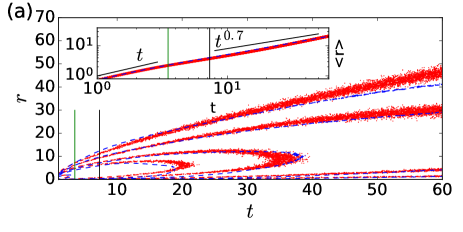
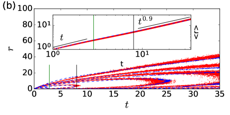
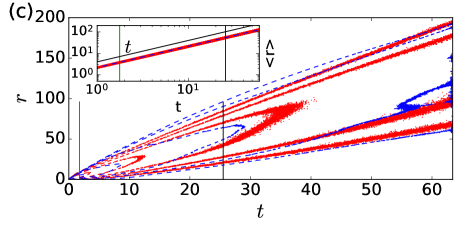
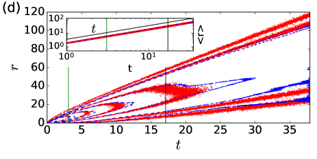
Figure 6: (Color online) Isocontours of $P(r,t)$ for the simulations (dashed blue lines) and for the model (dotted red lines), for (a) TG4, (b) TG8, (c) RND4, and (d) RND8. The inset show the mean horizontal displacement with the same line labels (power laws are shown as references, see text for details). Vertical lines (from left to right in all figures) indicate respectively the Eulerian $T_{e}$ and Lagrangian $T_{l}$ turnover times.

Figure 6 shows the probability density function $P(r,t)$ of a particle moving a horizontal distance $r$ after a time interval $t$, computed using all simulations and all available time increments. The insets in Fig. 6 show the mean horizontal displacement $\left<r\right>$ as a function of time (i.e., the first order moment of the PDFs), while Fig. 7 shows the mean horizontal quadratic displacement for all particles as a function of time, $\left<r^{2}\right>/(u_{\perp}^{2}T_{l}^{2})$ (i.e., the second order moment of the PDFs in Fig. 6), normalized by the mean squared perpendicular velocity and the Lagrangian turnover time using the scaling proposed in Aartrijk et al. (2008). The PDFs and the displacements are different depending on the forcing and on the time scale considered. At early times all simulations display $\left<r\right>\sim t$ and $\left<r^{2}\right>/(u_{\perp}^{2}T_{l}^{2})\sim(t/T_{l})^{2}$, with all curves in Fig. 7 collapsing in agreement with the scaling observed in Aartrijk et al. (2008). This indicates ballistic behavior at early times as in HIT Rast et al. (2016). However, at late times ($t/T_{l}>1$) the behavior of the TG and RND runs is clearly different, and differs from the scaling proposed in Aartrijk et al. (2008). In the TG runs, $\left<r\right>$ slows down but increases faster than $\sim t^{1/2}$ (see the insets in Fig. 6 and also the mean horizontal displacements normalized by the time $\left<r\right>/t$ in Fig. 7). This behavior at late times is not universal, as the dependence of $\left<r\right>$ with $t$ clearly varies with the level of stratification and with the forcing. The case of RND forcing (see Figs. 6 and 7) is even more interesting: $\left<r\right>\sim t$ and $\left<r^{2}\right>/(u_{\perp}^{2}T_{l}^{2})\sim(t/T_{l})^{2}$ even at late times, and the maximum of $P(r,t)$ in $r$ (see the PDFs in Fig. 6) displays a linear drift as $t$ increases.

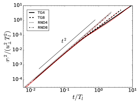
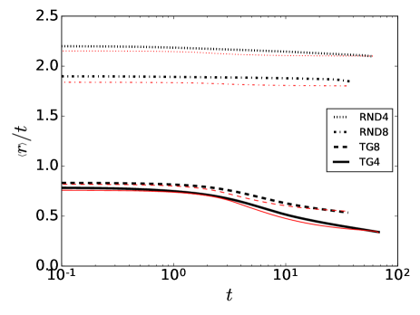
Figure 7: Left: mean horizontal quadratic dispersion for all runs (thick black curves), normalized by the product of the mean squared horizontal velocity $u_{\perp}^{2}$ and the squared Lagrangian turn-over time $T_{l}^{2}$, as a function of time normalized by $T_{l}$. The same quantity obtained from the model is shown by the thin (red) curves, using the same line labels as their corresponding simulation. The mean quadratic dispersion obtained from the model is in good agreement with all simulations. Right: mean horizontal displacements normalized by the time for all runs (thick black curves), such that curves are flat when $\left<r\right>\sim t$. Again, $\left<r\right>/t$ obtained from the model is shown in thin (red) curves.

In the horizontal case, the main difference between TG and RND runs is in the strength of the VSHW. In stratified flows, the anisotropic energy transfer towards modes with $k_{\perp}\approx 0$ results in the formation of strong horizontal winds with vertical shear Smith and Waleffe (2002); Marino et al. (2014). The flow is then given by weakly coupled horizontal layers, each with a mean horizontal velocity pointing in some direction. For RND forcing these winds develop in the entire domain, resulting in the almost ballistic motion of the particles observed in Fig. 1 (each particle is in a different layer, and thus the mean drift points in a different direction). However, in the TG case the coherent forcing imposes a large-scale structure that prevents the formation of mean winds, except in the few horizontal layers where shear is maximum and the forcing approaches zero. To illustrate this, Fig. 8 shows horizontal cuts of the horizontal velocity for runs TG4 and RND4 (for the sake of clarity, the velocity at $1\%$ of the grid points in the horizontal plane is shown). For RND4, on the average the horizontal velocity points towards a well defined direction, generating a coherent drift for all particles spending a sufficiently long time in this plane. For this run (as well as for the RND8 run), the same behavior is observed in other horizontal cuts at different heights. However, for the TG4 run (as well as for TG8, not shown) no clear mean wind is observed. As mentioned above, small mean winds can only develop for TG forcing in a few horizontal layers. This is further confirmed in Fig. 9, which shows the PDFs of the $\hat{x}$ component of the velocity $u_{x}$ (similar results are obtained for $u_{y}$), and of the r.m.s. horizontal velocity $u_{\perp}$, averaged over horizontal planes before computing the PDFs (the PDFs are also averaged in time). These PDFs thus quantify the probability of finding horizontal layers with mean horizontal winds, in particular, for runs TG4 and RND4. Note the RND4 run has stronger mean horizontal winds when compared with the TG4 run, while the TG4 run has larger probability of having layers with zero mean velocity, further confirming the observations made in Fig. 8.

Thus, we can conclude that in Fig. 7 there is a competition between transport and trapping by turbulent eddies (which is responsible for the mixing in the inertial range of HIT, and is also visible in Fig. 1) and the coherent drift (due to the VSHW in stratified turbulence). In the RND set of simulations the drift dominates the motion of all particles giving ballistic-like behaviour for all times, while in the TG set, as the drift is smaller and affects only a fraction of the particles, the competition results in a scaling in between ballistic and that observed in HIT. The VSHWs (and their different strengths depending on the level of stratification and type of forcing) can thus be expected to play an important role in the diffusion of particles, as observed in the atmosphere Saffman (1962); Smith (1965). The model we present next confirms this.

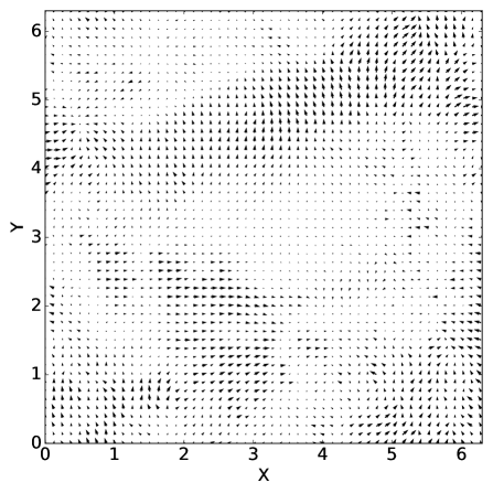
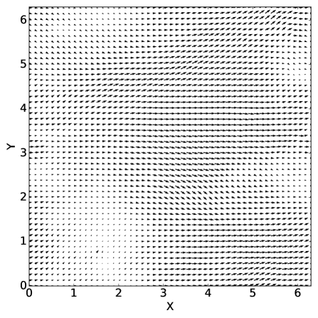
Figure 8: Horizontal cuts (in the $x$-$y$ plane, and at $z=0$) of the horizontal velocity at time $t=20$ for (left:) the TG4 run, and (right:) the RND4 run. Note the clear mean wind in the latter case, pointing approximately in the $\hat{x}$ direction. Other layers (i.e., for other values of $z$) have mean horizontal winds pointing in other directions.

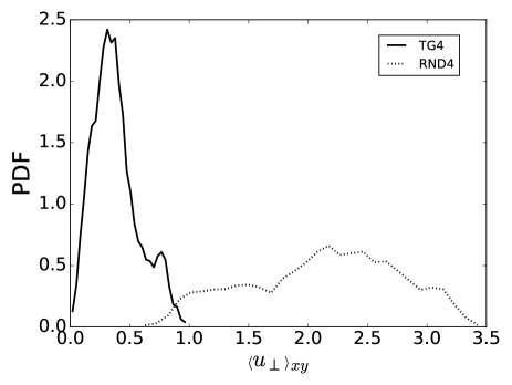
Figure 9: PDFs of the mean horizontal winds for the TG4 and RND4 runs. (Left:) PDF of $\left<u_{x}\right>_{xy}$, i.e., of the velocity in the $\hat{x}$ direction, $u_{x}$, averaged over the $x$ and $y$ coordinates, or equivalently, over planes at constant height. (Right:) Same for the r.m.s. horizontal velocity $u_{\perp}=(u_{x}^{2}+u_{y}^{2})^{1/2}$, also averaged over planes at constant height.

To capture the observed horizontal single-particle dispersion we use a continuous-time random walk model Rast et al. (2016), and extend it to build a model that can capture both trapping of particles by eddies as well as the drift caused by the VSHW. The motivation to use a CTEC random walk model is the following. While in HIT dispersion of particles is ballistic for short times and diffusive ($\left<r\right>\sim t^{1/2}$) for late times, it has been observed that the PDFs $P(r,t)$ show deviations from a Rayleigh distribution. In particular, at early times $P(r,t)$ displays a slightly smaller probability of particles having large displacements from their origins when compared with a Rayleigh distribution, while at late times a small excess of large displacements can be observed. This indicates that a simple random walk model is insufficient to capture the dynamics of the system. Using a point vortex model Rast and Pinton (2011), the early time behavior was shown to be associated with trapping of particles by the eddies, which then cannot travel as far as they could in a random walk. Naturally, the trapping time is a continuous random variable, whose distribution can be obtained, e.g., from comparisons with a point vortex model Rast et al. (2016). It is clear from Fig. 1 that trapping by eddies also plays a role in the horizontal displacement in our simulations, at least in the runs in which VSHW are not dominant. Thus, in our random walk model each particle is trapped in an eddy and displaces

$$dr_{t}=2r_{t}|\sin(\theta_{t})|$$ (14)

for a time $t_{t}$, where $r_{t}$ is the radius of the eddy, and

$$\theta_{t}=U_{t}t_{r}/r_{t}$$ (15)

is the central angle of motion of the particle while trapped, where $U_{t}$ is the Lagrangian particle velocity. The particle enters each eddy (i.e., each trap) with random phase. The model has no free parameters, and the probability distributions of $U_{t}$, $t_{t}$, and $r_{t}$ (with the sequence of random values for these quantities corresponding to the successive motion of a particle from one eddy to the next) are obtained from observations or from Kolmogorov theory of turbulence as follows. The probability density of finding an eddy of radius $r_{t}$ is taken to be Kolmogorovly distributed

$$P(r_{t})\sim r_{t}^{4/3}$$ (16)

for $r_{t}<L/2$, where $L$ is the Eulerian integral length of the flow as defined above. The assumption that the eddy distribution is Kolmogorovian is based on observations that the perpendicular velocity in stably stratified turbulence follows Kolmogorov scaling with the perpendicular wavenumber Riley and de Bruyn Kops (2003); Waite and Bartello (2004); Lindborg (2006); Brethouwer et al. (2007). The probability density of a given trapping time for a particular step $t_{t}$ is uniform between $0$ and $T_{e}$, where $T_{e}$ is the Eulerian turnover time Rast and Pinton (2011). Finally, the probability density of particle velocities $P(U_{t})$ is obtained from the PDF of the Lagrangian perpendicular velocity in the simulation (after subtracting the mean velocity associated with the drift caused by the VSHW). In each step of the random walk, a set of these variables is randomly generated, each chosen independently, and their values are kept constant over the trap duration $t_{t}$.

To this eddy-constrained random walk, a uniform drift $D_{t}=Wt_{t}$ is added to each particle, with the PDF of the wind $W$ (different for each particle) given by a bimodal Gaussian distribution corresponding to the best fit to the PDF of the VSHW (see Fig. 9) in each simulation. Note the VSHWs are different depending on the forcing, with larger values of $W$ in the RND runs, and lower values (and larger probability of having particles with $W\approx 0$) in the TG runs. The random walk is then constructed as the sum over steps of length $dr_{t}+D_{t}$.

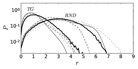
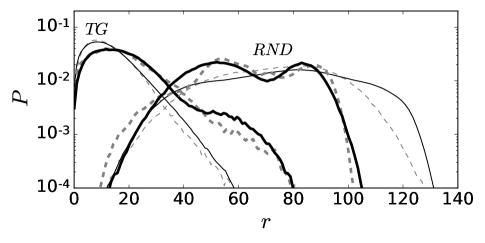
Figure 10: $P(r,t)$ at different times for the simulations (solid lines) and for the model (dashed lines). Thick lines correspond to flows with $N=4$, and thin lines to $N=8$. PDFs peaked at small values of $r$ are for TG forcing, while PDFs peaked at large values of $r$ are for RND forcing (as labeled). Left: $t=1.5$ ($t<T_{e}$). Right: $t=35$ ($t>T_{l}$).

The modeled $P(r,t)$ are also shown in Fig. 6, which are in good agreement with simulations. Note also that the model captures differences between TG and RND runs, differences between simulations with different values of the Brunt-Väisälä frequency $N$, as well as the anomalous behavior of $\left<r\right>$ and of $\left<r^{2}\right>$ (Fig. 7) at late times in all cases. The PDFs from the model and the simulations at two fixed times are also compared in Fig. 10. It is clear the PDFs are not Rayleigh, confirming turbulent transport in stratified flows cannot be modeled simply as a standard random walk. Moreover, two regimes are found for times shorter than the Eulerian turnover time $T_{e}$ and for times larger than the Lagrangian turnover time $T_{l}$. For $t<T_{e}$ trapping is more relevant than the drift, while for $t>T_{l}$ the drift dominates the dispersion giving very different PDFs in the TG and RND cases. Note that unlike HIT, the Lagrangian turnover times in all these simulations are larger than the corresponding Eulerian times, a result of a long term correlation in each particle trajectory caused by the drift by the VSHW. Indeed, the RND runs (which have stronger VSHW) have a larger separation between $T_{l}$ and $T_{e}$, and their separation also increases with increasing Brunt-Väisälä frequency $N$.

IV Conclusions

In this paper we studied single-particle dispersion in stably stratified turbulence using different forcing functions and Brunt-Väisälä frequencies. We showed that vertical dispersion is strongly reduced by the stratification, with the vertical Lagrangian velocity following a spectrum compatible with observations from wave-dominated geophysical flows Garrett and Munk (1975); Lien et al. (1998); D’Asaro and Lien (2000). Knowledge of this spectrum is enough to construct a random superposition of internal gravity waves which gives probability distribution functions of the waiting times of the Lagrangian particles in good agreement with the data, and mean vertical displacements in good agreement with the simulations up to the Brunt-Väisälä period in all simulations and for longer times in the simulations with random forcing. We also showed that horizontal dispersion differs from HIT and is strongly influenced by the large scale vertically sheared horizontal winds generated by the stratification Smith and Waleffe (2002); Marino et al. (2014); Clark di Leoni and Mininni (2015). Knowledge of the Eulerian typical flow velocity, of the Eulerian integral length, of the probability density function of the horizontal Lagrangian velocity, and of the strength of the horizontal winds is enough to build a continuous-time eddy-constrained random walk model, which takes into account particle trapping by eddies and drift by the mean winds, and which correctly reproduces the probability density function of the horizontal particle displacements in all simulations.

This model assumes that vertical displacements of the Lagrangian particles are negligible, or at least that they remain small across the time scales associated with the horizontal displacements, in such a way that each particle can be treated as being transported along a unique horizontal layer with a given horizontal wind. This is in good agreement with observations in our simulations, as well as with previous studies of Lagrangian transport and dispersion in stably stratified flows Nicolleau and Vassilicos (2000); Aartrijk et al. (2008). In particular, the observed mean squared vertical displacements confirm there is little mixing after one Brunt-Väisälä wave period, with saturation in the case of isotropic random forcing, and with a slow increase in the case of Taylor-Green forcing. However, it may be the case that for stronger turbulence, or for weaker stratification (i.e., for larger values of the buoyancy Reynolds number), vertical mixing can be stronger and cause particles to change layers on faster time scales. Moreover, our results for two different forcing functions indicate that the local gradient Richardson number may be a better indicator of such a change in behavior. A detailed parametric study of vertical transport for moderate values of the Froude number and for larger Reynolds numbers is left for future work.

For the range of parameters considered in this study, the results show that single-particle dispersion in stably stratified fluids departs significantly from the behavior observed in HIT, which has strong implications for the study of transport in geophysical flows. In particular, transport at times larger than the Lagrangian turnover time is not universal, and strongly dependent on the presence or not of horizontal winds. Thus, even the mean displacement of the particles cannot be modeled by a single power law of time, and may not be self-similar. As mentioned above, the models we presented capture this behavior and yield results in good agreement with numerical simulations. For the range of parameters considered here, the model indicates that while vertical transport is mostly mediated by a random superposition of internal gravity waves, proper capturing of the horizontal transport requires a superposition of a random walk with trapping, with a mean drift caused by horizontal winds, which are dependent on the forcing, on the stratification level, and in geophysical scenarios can also be affected by topography and other factors. Finally, the model provides a statistical prediction of moments of the PDF of dispersion without the need of explicit simulation of the turbulent flow and of individual particle trajectories. Note this is of particular importance for the modeling of geophysical flows. While in recent years state of the art simulations allowed studies with very high spatial resolution of atmospheric and oceanic flows, forecasts and large scale modeling require ensembles of runs which are performed at lower resolutions and which cannot resolve the small scale turbulence. As a result, the development of statistical models not only provides a deeper insight into the mechanisms behind particle dispersion, but can also allow the development of subgrid scale models of turbulent particle transport and mixing.

Appendix A Horizontal dispersion with Kolmogorov forcing

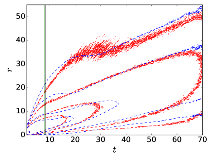
Figure 11: (Color online) Left: Mean horizontal dispersion as a function of time for a run with Kolmogorov forcing and $N=8$ (thick black line). Dispersion in the random walk model is shown by the thin (red) line. Right: Isocontours of $P(r,t)$ for the simulation (dashed blue curves) and for the model (dotted red curves). Vertical lines (from left to right) indicate respectively the Eulerian $T_{e}$ and Lagrangian $T_{l}$ turnover times.

To further test the model for horizontal dispersion we briefly present here a $512^{3}$ simulation with Brunt-Väisälä frequency $N=8$, the same parameters as in the other simulations ($\nu=\kappa=8\times 10^{-4}$ and Schmidt number $\textrm{Sc}=1$), but with Kolmogorov forcing. To force at the same scales as in the previous simulations, we apply the Kolmogorov forcing at $k=1$ and $2$ (see, e.g., Rollin et al. (2011)) and use

$${\bf f}=f_{0}\left[\sin(y)+\sin(2y)\right]\hat{x}.$$ (17)

While in RND forcing all three components of the velocity field are forced and the forcing is isotropic, and in TG forcing both horizontal components of the velocity are forced, in Kolmogorov forcing only one component of the velocity is forced, resulting in the turbulent steady state in an anisotropic flow even in the horizontal plane. As an example, in the turbulent steady state the r.m.s. Eulerian velocity in the $x$ direction is almost three times larger than the r.m.s. value of the Eulerian velocity in the $y$ direction.

For this simulation, as for the previous simulations, we studied the mean horizontal dispersion and the probability distribution $P(r,t)$ of finding a particle at a given distance $r$ at time $t$ from its original location (see Fig. 11). Using the typical value of the horizontal Eulerian velocity (averaged in the $x$ and $y$ directions), the Eulerian turnover time, the PDF of the Lagrangian velocity of the particles, and the typical amplitude of the horizontal winds, we also computed the random walk model (see also Fig. 11). Considering the strong horizontal anisotropy in this flow, which is different from the other forcing functions studied in this work, the model is in good agreement with the simulations, especially for the PDF of the displacements $P(r,t)$.

The mean horizontal dispersion in the simulation shows ballistic behaviour at early times ($\left<r\right>\sim t$), and slows down at later times, albeit less than in the TG simulations. Again, there is a competition between diffusion and trapping by the turbulent eddies and the drift by the horizontal winds, which in this simulation are weaker than in the RND runs but stronger than in the TG runs. The PDF $P(r,t)$ has an excess of particles that travel far from their origin at early times (up to $t\approx 30$), which can be seen as a bump in the isocontours. Then, horizontal winds give almost linear isocontours in time. The model, without any modification, can capture for this flow both features and the overall shape of the PDF.

References

- Yeung (2002) P. K. Yeung, “Lagrangian investigations of turbulence,” Annu. Rev. Fluid Mech. 34, 115–142 (2002).
- Toschi and Bodenschatz (2009) F. Toschi and E. Bodenschatz, “Lagrangian properties of particles in turbulence,” Annu. Rev. Fluid Mech. 41, 375–404 (2009).
- Zimmermann et al. (2010) R. Zimmermann, H. Xu, Y. Gasteuil, M. Bourgoin, R. Volk, J.-F. Pinton, E. Bodenschatz, and International Collaboration for Turbulence Research, “The lagrangian exploration module: An apparatus for the study of statistically homogeneous and isotropic turbulence,” Rev. Sci. Instrum. 81, 055112 (2010).
- Falkovich et al. (2012) G. Falkovich, H. Xu, A. Pumir, E. Bodenschatz, L. Biferale, G. Boffetta, A. S. Lanotte, F. Toschi, and International Collaboration for Turbulence Research, “On lagrangian single-particle statistics,” Phys. Fluids (1994-present) 24, 055102 (2012).
- Pumir et al. (2016) A. Pumir, H. Xu, E. Bodenschatz, and R. Grauer, “Single-particle motion and vortex stretching in three-dimensional turbulent flows,” Phys. Rev. Lett. 116, 124502 (2016).
- Bec et al. (2006) J. Bec, L. Biferale, M. Cencini, A. S. Lanotte, and F. Toschi, “Effects of vortex filaments on the velocity of tracers and heavy particles in turbulence,” Phys. Fluids 18, 081702 (2006).
- Thalabard et al. (2014) S. Thalabard, G. Krstulovic, and J. Bec, “Turbulent pair dispersion as a continuous-time random walk,” J. Fluid Mech. 755, R4 (2014).
- Wyngaard (1992) J. C. Wyngaard, “Atmospheric turbulence,” Annu. Rev. Fluid Mech. 24, 205–234 (1992).
- Biferale et al. (2016) L. Biferale, F. Bonaccorso, I. M. Mazzitelli, M. A. T. van Hinsberg, A. S. Lanotte, S. Musacchio, P. Perlekar, and F. Toschi, “Coherent structures and extreme events in rotating multiphase turbulent flows,” Phys. Rev. X 6, 041036 (2016).
- Liechtenstein et al. (2005) L. Liechtenstein, F. S. Godeferd, and C. Cambon, “Nonlinear formation of structures in rotating stratified turbulence,” J. Turbul. 6, N24 (2005).
- Liechtenstein et al. (2006) L. Liechtenstein, F. S. Godeferd, and C. Cambon, “The role of nonlinearity in turbulent diffusion models for stably stratified and rotating turbulence,” Int. J. Heat and Fluid Flow Special Issue of The Fourth International Symposium on Turbulence and Shear Flow Phenomena - 2005, 27, 644–652 (2006).
- Kimura and Herring (1996) Y. Kimura and J. R. Herring, “Diffusion in stably stratified turbulence,” J. Fluid Mech. 328, 253–269 (1996).
- Aartrijk et al. (2008) M. van Aartrijk, H. J. H. Clercx, and K. B. Winters, “Single-particle, particle-pair, and multiparticle dispersion of fluid particles in forced stably stratified turbulence,” Phys. Fluids (1994-present) 20, 025104 (2008).
- Sozza et al. (2016) A. Sozza, F. De Lillo, S. Musacchio, and G. Boffetta, “Large-scale confinement and small-scale clustering of floating particles in stratified turbulence,” Phys. Rev. Fluids 1, 052401 (2016).
- Kaneda and Ishida (2000) Y. Kaneda and T. Ishida, “Suppression of vertical diffusion in strongly stratified turbulence,” J. Fluid Mech. 402, 311–327 (2000).
- Sagaut and Cambon (2008) P. Sagaut and C. Cambon, Homogeneous Turbulence Dynamics (Cambridge University Press, Cambridge, 2008).
- Billant and Chomaz (2001) P. Billant and J.-M. Chomaz, “Self-similarity of strongly stratified inviscid flows,” Phys. Fluids 13, 1645–1651 (2001).
- Smith and Waleffe (2002) L. M. Smith and F. Waleffe, “Generation of slow large scales in forced rotating stratified turbulence,” J. Fluid Mech. 451, 145–168 (2002).
- Marino et al. (2014) R. Marino, P. D. Mininni, D. L. Rosenberg, and A. Pouquet, “Large-scale anisotropy in stably stratified rotating flows,” Phys. Rev. E 90, 023018 (2014).
- Clark di Leoni and Mininni (2015) P. Clark di Leoni and P. D. Mininni, “Absorption of waves by large-scale winds in stratified turbulence,” Phys. Rev. E 91, 033015 (2015).
- Terry (2000) P. W. Terry, “Suppression of turbulence and transport by sheared flow,” Rev. Mod. Physics 72, 109 (2000).
- Shapiro (1980) M. A. Shapiro, “Turbulent mixing within tropopause folds as a mechanism for the exchange of chemical constituents between the stratosphere and troposphere,” J. Atmos. Sci. 37, 994–1004 (1980).
- Davis and Yan (2004) A. Davis and X.-H. Yan, “Hurricane forcing on chlorophyll-a concentration off the northeast coast of the U.S.” Geophys. Res. Lett. 31, L17304 (2004).
- D’Asaro and Lien (2000) E. A. D’Asaro and R.-C. Lien, “Lagrangian measurements of waves and turbulence in stratified flows,” J. Phys. Oceanogr. 30, 641–655 (2000).
- Garrett and Munk (1975) C. Garrett and W. Munk, “Space-time scales of internal waves: A progress report,” J. Geophys. Res. 80, 291–297 (1975).
- Lien et al. (1998) R.-C. Lien, E. A. D’Asaro, and G. T. Dairiki, “Lagrangian frequency spectra of vertical velocity and vorticity in high-reynolds-number oceanic turbulence,” J. Fluid Mech. 362, 177–198 (1998).
- Rast et al. (2016) M. P. Rast, J.-F. Pinton, and P. D. Mininni, “Turbulent transport with intermittency: Expectation of a scalar concentration,” Phys. Rev. E 93, 043120 (2016).
- Mininni et al. (2011) P. D. Mininni, D. Rosenberg, R. Reddy, and A. Pouquet, “A hybrid mpi–openmp scheme for scalable parallel pseudospectral computations for fluid turbulence,” Parallel Computing 37, 316–326 (2011).
- Yeung and Pope (1988) P. K. Yeung and S. B Pope, “An algorithm for tracking fluid particles in numerical simulations of homogeneous turbulence,” Journal of Computational Physics 79, 373–416 (1988).
- Riley and de Bruyn Kops (2003) J. J. Riley and S. M. de Bruyn Kops, “Dynamics of turbulence strongly influenced by buoyancy,” Physics of Fluids 15, 2047–2059 (2003).
- Ivey et al. (2008) G. N. Ivey, K. B. Winters, and J. R. Koseff, “Density stratification, turbulence, but how much mixing?” Annual Review of Fluid Mechanics 40 (2008).
- Rosenberg et al. (2015) D. Rosenberg, A. Pouquet, R. Marino, and P. D. Mininni, “Evidence for Bolgiano-Obukhov scaling in rotating stratified turbulence using high-resolution direct numerical simulations,” Physics of Fluids 27, 055105 (2015).
- D’Asaro et al. (2007) E. A. D’Asaro, R.-C. Lien, and F. Henyey, “High-frequency internal waves on the oregon continental shelf,” Journal of physical oceanography 37, 1956–1967 (2007).
- Rorai et al. (2014) C. Rorai, P. D. Mininni, and A. Pouquet, “Turbulence comes in bursts in stably stratified flows,” Phys. Rev. E 89, 043002 (2014).
- Saffman (1962) P. G. Saffman, “The effect of wind shear on horizontal spread from an instantaneous ground source,” Q.J.R. Meteorol. Soc. 88, 382–393 (1962).
- Smith (1965) F. B. Smith, “The role of wind shear in horizontal diffusion of ambient particles,” Q.J.R. Meteorol. Soc. 91, 318–329 (1965).
- Rast and Pinton (2011) M. P. Rast and J.-F. Pinton, “Pair dispersion in turbulence: The subdominant role of scaling,” Phys. Rev. Lett. 107, 214501 (2011).
- Waite and Bartello (2004) M. L. Waite and P. Bartello, “Stratified turbulence dominated by vortical motion,” Journal of Fluid Mechanics 517, 281–308 (2004).
- Lindborg (2006) E. Lindborg, “The energy cascade in a strongly stratified fluid,” Journal of Fluid Mechanics 550, 207–242 (2006).
- Brethouwer et al. (2007) G. Brethouwer, P. Billant, E. Lindborg, and J.-M. Chomaz, “Scaling analysis and simulation of strongly stratified turbulent flows,” Journal of Fluid Mechanics 585, 343–368 (2007).
- Nicolleau and Vassilicos (2000) F. Nicolleau and J. C. Vassilicos, “Turbulent diffusion in stably stratified non-decaying turbulence,” J.Fluid Mech. 410, 123–146 (2000).
- Rollin et al. (2011) B. Rollin, Y. Dubief, and C. R. Doering, “Variations on Kolmogorov flow: turbulent energy dissipation and mean flow profiles,” J. Fluid Mech. 670, 204–213 (2011).