The Pristine survey II: –
a sample of bright stars observed with FEROS

Abstract

Extremely metal-poor (EMP) stars are old objects formed in the first Gyr of the Universe. They are rare and, to select them, the most successful strategy has been to build on large and low-resolution spectroscopic surveys. The combination of narrow- and broad band photometry provides a powerful and cheaper alternative to select metal-poor stars. The on-going Pristine Survey is adopting this strategy, conducting photometry with the CFHT MegaCam wide field imager and a narrow-band filter centred at 395.2 nm on the Ca ii-H and -K lines. In this paper we present the results of the spectroscopic follow-up conducted on a sample of 26 stars at the bright end of the magnitude range of the Survey ($g\la 15$), using FEROS at the MPG/ESO 2.2 m telescope. From our chemical investigation on the sample, we conclude that this magnitude range is too bright to use the SDSS $gri$ bands, which are typically saturated. Instead the Pristine photometry can be usefully combined with the APASS $gri$ photometry to provide reliable metallicity estimates.

1 Introduction

Extremely metal-poor (EMP, [Fe/H]$\leq-3$) stars are old objects that formed from a gas cloud that did not yet have the time to be enriched in metals by supernovae explosions, the last stage of the evolution of the massive stars. This low metal-content of the gas was the typical chemical composition of the pristine Universe, at redshift $z>5$, i.e. more than 12.5 Gyr ago (see e.g. Pallottini et al. 2014, Figure 2). Among the stars formed from metal-poor clouds at this early stage of the Universe, only those with low mass (mass lower than the Solar mass) are still observable today because their life-time is longer than the age of the Universe. Stars more massive than the Sun had time to evolve and at present they are underluminous compact objects: neutron stars or black holes, remnants of type II supernovae explosion for the most massive stars, or white dwarfs for the less massive stars. The EMP stars are very rare objects and, in order to find them, large amounts of data have to be gathered and analysed. Several projects focused on the search and chemical investigations of EMP stars are based on the analysis of low-resolution spectra obtained by large surveys in order to select the most promising candidates to observe at medium- or high-resolution (see e.g. Beers et al. 1985, 1992; Christlieb et al. 2008; Caffau et al. 2013).

Observing stars photometrically is much faster than to take spectra; one can also go deeper and observe fainter objects with the same telescope size and integration time. A classical metallicity-sensitive colour is $U-B$, that however saturates its sensitivity at metallicity around –2.0. Recently Monelli et al. (2013) have introduced the index $C\_UBI=(U-B)-(B-I)$ that turned out to be very useful to identify multiple populations in Globular Clusters and dwarf galaxies (Monelli et al. 2014). Fabrizio et al. (2015) have shown that this index is also metallicity sensitive and one may expect similar performances also for analogous $C\_ugr$ or $C\_ugi$ colours. Yet their sensitivity still has to be tested at metallicities below –3.0.

The spectra of EMP stars are characterised by a small number of weak metallic absorption lines. Even the strongest metallic absorption lines in the Solar spectrum disappear or become extremely weak in the spectrum of an EMP star. When a low-resolution spectrum (resolving power of: $R\approx$ 2000) of a metal-poor star is analysed, the lines belonging to the Mg ib and the infra-red Ca ii triplets are usually detected, but in the EMP regime these lines are usually not detectable. The only feature that is always present is the strong Ca ii-K absorption line at 392 nm. This line is sometimes the only metallicity indicator to select EMP candidates from low-resolution spectra. This feature is so strong that its presence is also detectable in photometric observations. To make the signature of this line clear, narrow-band photometry centred at about 395.2 nm is the best solution and EMP candidates can be efficiently and reliably selected.

The use of a narrow band filter centred on the Ca ii H and K lines, in conjunction with Strömgren intermediate bands, as a means to obtain metallicity estimates down to very low metallicities is well established (Anthony-Twarog et al. 1991; Twarog & Anthony-Twarog 1995; Anthony-Twarog & Twarog 1998; Twarog et al. 2007, and references therein). The Pristine Project (Starkenburg et al. 2017) extends this technique by coupling a narrow band Ca ii H and K filter (CaHK) to the broadband survey $gri$ photometry, e.g. the SDSS bands (York et al. 2000). To do this it uses the wide-field imager MegaCam (Boulade et al. 2003) mounted on the Canada France Hawaii Telescope (CFHT). We are performing follow-up spectroscopy with several telescope/spectrograph combinations at both low ($R\sim 2000$) and high ($R>40000$) spectral resolution. The spectra will allow us to derive the metallicities of the stars in order to better calibrate the photometric indices (see Youakim et al. in prep.). We present here the chemical analysis of a sample of 26 among the brightest objects that have been observed with FEROS (Kaufer & Pasquini 1998; Avila et al. 2004) at the MPG/ESO 2.2 m telescope at La Silla.

2 Observations and data reduction

The MPG/ESO 2.2 m FEROS data were taken during a visitor mode observing run from April 13 to 16, 2016. They were automatically reduced using the FEROS pipeline (Kaufer et al. 2000). Typically, three sub-exposures were taken per object and these are combined using the IRAF combine task using an average sigma clipping rejection. Any pixels which still lie more than 3$\sigma$ from the continuum in the combined spectrum are clipped to remove remaining cosmic rays. FEROS observes with a simultaneous sky fiber and we follow the same procedure for these spectra before subtracting the sky spectrum from the object.

Finally, the object spectrum is shifted to rest wavelengths coss-correlating a synthetic spectrum for the Mg ib region of a typical EMP giant, which has been created using an (OS)MARCS stellar atmosphere and the Turbospectrum code (Alvarez & Plez 1998; Gustafsson et al. 2008; Plez 2008).

3 Calibration of the HK filter on the AB system

The concept of AB magnitude was introduced by Oke & Gunn (1983) who defined that magnitude zero in any band corresponds to the magnitude of an ideal body with constant flux density at any wavelength, such that $f^{0}_{\nu}=\rm 3.631\times 10^{-23}WHz^{-1}m^{-2}$. The SDSS $ugriz$ system is such an AB system.

If we denote as $S_{\lambda}$ the instrument response function of our system (including filter transmission, transmission of the system optics and quantum efficiency of the detector) and $f_{\lambda}$ the flux of the object to be measured we define

$$m_{AB,S_{\lambda}}=-2.5\log\left(\int\lambda f_{\lambda}S_{\lambda}d\lambda\right)+2.5\log\left(\int\lambda f^{0}_{\nu}S_{\lambda}d\lambda\right)$$ (1)

The second term of the right hand-side of the equation ensures that $m_{AB,S_{\lambda}}$ is zero for the ideal constant flux density object and it can be easily computed taking into account that $f^{0}_{\lambda}=f^{0}_{\nu}c/\lambda^{2}$, where $c$ is the speed of light in vacuum. We use as $S_{\lambda}$ the response function described in Starkenburg et al. (2017), that is an average of the response function across the MegaCam field of view. This takes into account the filter transmission, the quantum efficiency of the CCD’s and a model of the atmospheric transmission. With this $S_{\lambda}$ the zero-magnitude constant is equal to $-9.9795$.

This definition is useful for synthetic photometry, however it does not solve the practical problem of transforming instrumental magnitudes to the standard system. This is achieved through observations of standard stars. The SDSS system defined 4 primary standard stars (Fukugita et al. 1996), the magnitudes of these stars are derived by integrating the flux given in that paper, multiplied by the SDSS instrument response function. Table 7 of Fukugita et al. (1996) provides the $ugriz$ magnitudes of the four primary standards.

For the CFHT–MegaCam Ca ii H and K filter, the magnitudes of the 4 primary SDSS standards are given in Table 1.

Table 1: $CaHK$ magnitudes of the primary standard stars.

HD 84937	HD 19445	BD+26∘ 2606	BD +17∘ 4708
8.7745	8.6615	10.2692	10.0545

In the SDSS photometry, the magnitudes of the primary standard stars are used to transform the instrumental magnitudes observed with the SDSS Monitor Telescope (60 cm aperture) onto the standard system, these are then tied to the secondary standards (Smith et al. 2002). Efforts are under way to observe the SDSS primary standards with a smaller telescope and a similar filter, that can be cross-calibrated with the CFHT MegaCam CaHK filter. However, for the time being we do not yet know precisely the absolute zero point of the CFHT $CaHK$ photometry. We could not use the standard stars of the $hk$ system (Anthony-Twarog et al. 1991; Twarog & Anthony-Twarog 1995; Anthony-Twarog & Twarog 1998) or the ones more recently established by Lee et al. (2009) and Calamida et al. (2011) because they are all too bright to be observed directly with the CFHT 3.6 m telescope. In addition, since we are really interested in the colours obtained combining the $CaHK$ photometry with SDSS $gri$, the above-mentioned standard stars are too bright for SDSS as well. Finally, since the CaHK filters on the different telescopes are different, the use of the established standards would require a careful cross-calibration, and likely also a dedicated observational campaign.

We computed synthetic photometry from the fluxes of the grid of ATLAS (Kurucz 2005) models of Castelli & Kurucz (2003), with the above-defined zero point, we then applied a $-0.13$ mag offset, as described in Starkenburg et al. (2017) to match the internal survey zero-point.

4 Analysis

4.1 Selection from photometry

The combination of the narrow-band filter CaHK and broad-band Sloan filters allows us to distinguish stars with different metallicities, as shown in Figure 3 of Starkenburg et al. (2017). In Fig. 1 a linear combination of broad-band Sloan filters and the CaHK as a function of the colour $(g-i)_{0}$ is compared to synthetic colours. From the plot, all stars in our sample, with the exception of one, are expected to be metal-poor, ${\rm[Fe/H]}<-1.0$. However, all of these stars are at the bright-end for the SDSS Survey and they all have a flag of saturation for the individual filters. We decided to observe them anyway because the global flag SDSS “clean” was set. At the time of this first spectroscopic follow-up, SDSS photometry was the reference, which led to the selection of stars. However, the first abundance investigation on this sample of stars revealed metallicities higher than expected. In order to understand this result, the first step was to check the photometry. We then decided to use the $gri$ photometry of the APASS survey (Henden et al. 2015; Henden & Munari 2014; Henden et al. 2009, https://www.aavso.org/apass) instead. The colour-colour plot in Fig. 2 is thus obtained: the majority of the stars, which are metal-rich ([Fe/H]$>-1.0$) according to the chemical analysis described below (see Sect.4.2), move down to a more appropriate place in the colour-colour space in the figure, close to the theoretical values corresponding to solar metallicity and metal-poor stars are in the range of metal-poor theoretical colours. The large uncertainties in the colours are dominated by the uncertainties in the APASS bands; the CaHK band has a small uncertainty, negligible in the vertical error bars in Fig. 2.

At the time we selected and observed the stars, the Pan-STARRS photometry (Tonry et al. 2012) was not available. It is our plan to use this survey for the future star selection.

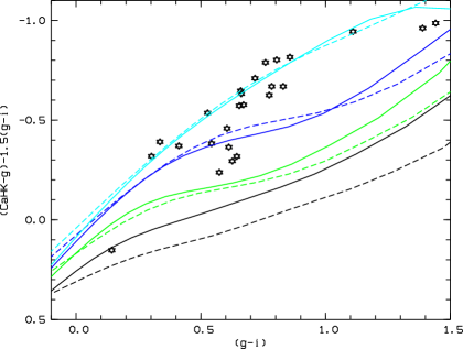
Figure 1: The sample stars are represented as black stars. The colours are derived from Pristine and SDSS photometry. Solid and dashed lines represent the theoretical colours for $\log{\rm g}$ of 2.5 and 4.5, respectively. Black lines are for solar metallicity, green lines for [Fe/H]=–1.0, blue lines for [Fe/H]=–2.0, light blue for [Fe/H]=–4.0.

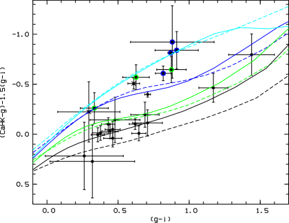
Figure 2: The sample stars are represented as black dots. The colours are derived from Pristine and APASS photometry. The stars with a larger blue dots are stars with $[{\rm Fe/H}]<-2.0$, the green ones $-2.0<[{\rm Fe/H}]<-1.0$, [Fe/H] is from Table 2. Crosses represent spectra that have not been analysed. Lines are as in Fig. 1.

In Fig. 3, we used the broad-band $r$ filter instead of $i$ and we can see a clearer separation of metal-poor and solar-metallicity stars. In addition in this case the metallicity derived from the spectra puts the stars in the plot closer to the corresponding locus defined by theoretical colours.

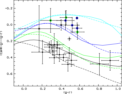
Figure 3: The sample stars are represented as black dots. The colours are derived from APASS photometry. The stars with a larger blue dots are stars with $[{\rm Fe/H}]<-2.0$, the green ones $-2.0<[{\rm Fe/H}]<-1.0$, [Fe/H] is from Table 2. Crosses represent spectra that nave not been analysed. Theoretical colour are as in Fig. 2.

4.2 Chemical analysis

To derive the effective temperatures of the stars, taking advantage of the APASS filters, we used the calibrations from Ivezić et al. (2008). These authors provide the following expressions to derive ${\rm T}_{\rm eff}$:

1. $\log{\rm T_{\rm eff}}=3.882-0.316\left(g-r\right)_{0}+0.0488\left(g-r\right)_{0}^{2}+0.0283\left(g-r\right)_{0}^{3}$ applicable for $-0.3<\left(g-r\right)_{0}<1.3$;

2. ${5040\,{\rm K}\over{\rm T_{\rm eff}}}=0.532\left(g-r\right)_{0}+0.654$ in good agreement with expression (1).

We derive the ${\rm T}_{\rm eff}$ from these two expressions. After iterations of the spectrum analysis, we used expression 1 for unevolved stars and expression 2 for evolved stars. The absolute average difference among the two ${\rm T}_{\rm eff}$ scales 30 K, and 21 stars have a difference in the two ${\rm T}_{\rm eff}$ estimates smaller than 30 K. For the RR Lyr Pristine_225.8227+14.2933 and for the cool dwarf Pristine_255.0531+10.7488 the differences are slightly larger than 100 K.

With a fixed ${\rm T}_{\rm eff}$ we ran the code MyGIsFOS using a grid of synthetic spectra computed with turbospectrum (Alvarez & Plez 1998; Plez 2012), based on the grid of OSMARCS models and line-lists provided by the GES collaboration (Smiljanic et al. 2014; Heiter et al. 2015) and already used by Duffau et al. (2017). MyGIsFOS is a code that analyses stellar spectra in order to derive the stellar parameters and the chemical composition simulating a traditional abundance analysis; details can be found in Sbordone et al. (2014). HE 1207-3108 has been observed in the same observation programme, in order to check the accuracy of our analysis. The spectrum has a low signal-to-noise ratio (SNR of 25 per pixel at 500 nm) so that only few lines are detected in the spectrum of this metal-poor star. We adopted the stellar parameters from Yong et al. (2013) (${\rm T}_{\rm eff}$/$\log{\rm g}$ of 5294 K/2.85) and a micro-turbulence of 1.0 km/s, close to the 0.9 km/s adopted by Yong et al. (2013). Analysing this spectrum as the others of the sample, we derive ${\rm[Fe/H]}=-2.78\pm 0.20$ to be compared to ${\rm[Fe/H]}=-2.70$ from Yong et al. (2013). We also agree with the result of Yong et al. (2013) on a low Ca abundance, but we can only detect two lines. We also analysed the spectrum of HE 1005-1439 that unfortunately has a low SNR of 10 at 500 nm. By adopting the stellar parameters from Aoki et al. (2007) (${\rm T}_{\rm eff}=5000$ K, $\log{\rm g}=1.9$ and a micro-turbulence of 2.0 km/s) we obtain from two lines of neutral iron [Fe/H]$=-3.08\pm 0.12$, in good agreement with [Fe/H]=–3.17 of Aoki et al. (2007).

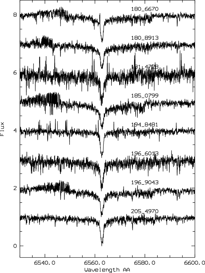
Figure 4: H$\alpha$ for eight of the analysed stars.

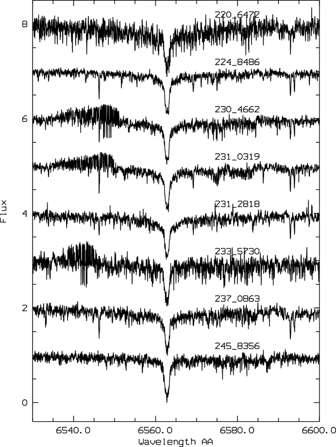
Figure 5: H$\alpha$ for the other eight of the analysed stars.

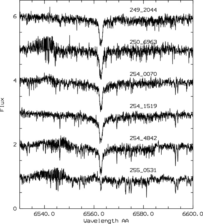
Figure 6: H$\alpha$ for the last six analysed stars.

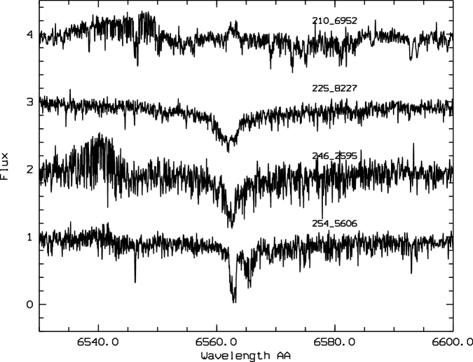
Figure 7: Four peculiar H$\alpha$ profiles.

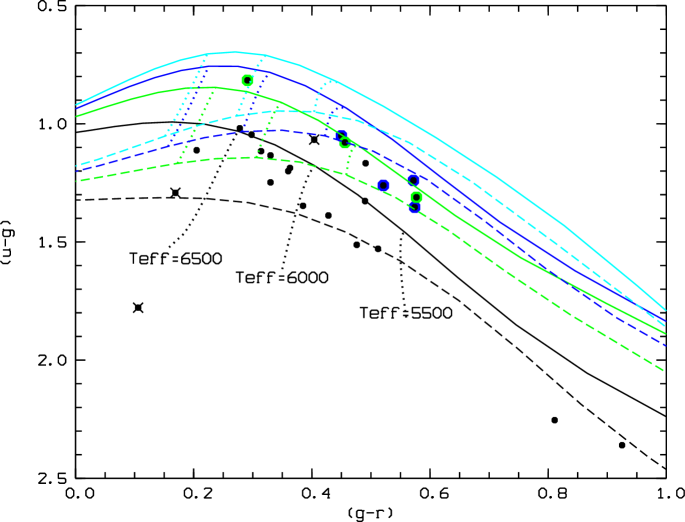
Figure 8: The $(u-g)$ vs. $(g-r)$ diagram for our program stars. Overlayed synthetic colours for [M/H]=0.0 (black), [M/H]=–1.0 (green), [M/H]=–2.0 (blue) and [M/H]=–4.0 (cyan), for log g =2.5 (solid lines) and log g =4.5 (dashed lines). [M/H] is the metallicity of the model, note that all the metal-poor models are enhanced by +0.4 dex in $\alpha$-elements.

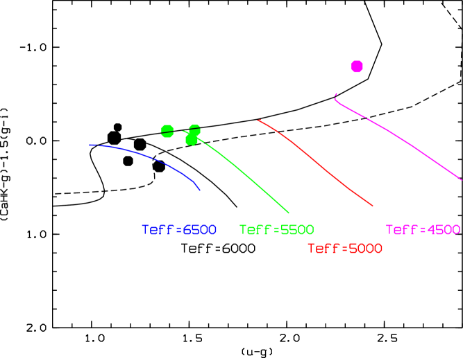
Figure 9: The $(u-g)$ vs. $(CaHK-g)-1.5(g-r)$ diagram for our program stars with metallicity [M/H]$\approx 0.0$. The solid line corresponds to synthetic colours for log g = 2.5 and the dashed lines to log g = 4.5. Each star is colour coded with the closest T_eff and the symbol size is proportional to log g.

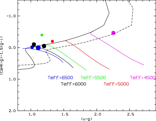
Figure 10: Like Fig. 9, but for [M/H]=-0.5.

For the stars in the sample, the surface gravity is based on the iron ionisation balance; we also systematically compared the wings of the Mg I b triplet of the observed spectra to synthetic profile computed with the derived surface gravity as an extra-check on the surface gravity. The micro-turbulence is derived from the agreement between the Fe abundance derived from weak and strong Fe i lines. For some spectra the signal-to-noise ratio is too poor to derive surface gravity and micro-turbulence and we fix the stellar parameters as follows: surface gravity looking only at the wings of the Mg I b triplet and the micro-turbulence using values of stars already known and analysed in the literature with similar atmospheric parameters (e.g. Santos et al. 2005; Ecuvillon et al. 2004; François et al. 2007).

In Table 2, we provide the stellar parameters for the programme stars included the barycentric radial velocities derived from our spectra. Pristine 225.8227+14.2933 is already known in the literature (SDSS J150317.44+141735.7) and is classified as an RR Lyr type (see Drake et al. 2013). We do not know at which phase this star has been observed and we cannot derive the effective temperature from the photometry or the wings of H$\alpha$. The quality of the spectrum is mediocre, with a signal-to-noise ratio (SNR) of 24 at 540 nm. We decided to look at the very few lines detected and we chose a particular couple of Fe i lines (at 540 and 543 nm) whose depth ratio depends on the stellar temperature. From this diagnostic we would derive a ${\rm T}_{\rm eff}$ of about 5400 K. But when we examined at the line-to-line scatter of the four Fe i lines, the lowest value is found for a ${\rm T}_{\rm eff}$ of about 6600 K. In Table 2 we provide values for both cases. We are confident that this star is metal-poor, with an iron abundance of the order of or below 1/100 the Solar value, but we are not able to give a better determination.

Pristine 246.2595+11.8378 is within $3^{\prime\prime}$ from CSS J162502.2+115017, also an RR Lyr type star (Drake et al. 2013; Abbas et al. 2014). With a poor spectrum quality, SNR of 10 at 540 nm, we are not able to derive any information on the chemical composition. Also the spectrum of Pristine 181.4728+15.5306 is of poor quality and did not allow us to derive any chemical information of the star.

The use of $hk$ index to derive metallicities of RR Lyr stars has already been demonstrated both for the field (Baird 1996) and cluster (Rey et al. 2000) variables. Our $CaHK$ photometry can provide similar performances. In our survey we expect to find EMP RR Lyr stars, such as are already known to exist (Wallerstein et al. 2009; Hansen et al. 2011) along with non-pulsating HB-stars (Preston et al. 2006; Çalışkan et al. 2014).

Table 2: Programme stars coordinates and atmospheric parameters. To derive [Fe/H] the iron Solar abundance is from Caffau et al. (2011).

Star	R.A.	Dec.	g0	Vrad	Teff	Logg	$\xi$	[Fe/H]	Comment
	deg	deg	mag	[km/s]	K	cgs	km/s	dex
Pristine 180.6670+13.3324	180.6669617	+13.33239746	13.9	+30.0	6210	4.54	0.94	$-0.60$	A(Li)${}_{\rm 1DLTE}=2.58$
Pristine 180.8913+11.3199	180.8912811	+11.3199358	13.9	+15.3	6290	4.28	1.00	$-0.51$	(Y), $\xi$ fixed
Pristine 181.4728+15.5306	181.4727936	+15.53064156	15.2	–18.5					(Y), Only noise
Pristine 185.0799+14.6464	185.0799103	+14.64640236	14.1	+162.5	6240	3.24	1.50	$-1.48$	(Y), $\xi$ fixed
Pristine 194.8481+11.5875	194.8481293	+11.58754444	14.7	+119.7	5260	3.00	1.50	$-2.64$	(Y), log g and $\xi$ fixed
Pristine 196.6013+15.6768	196.6013336	+15.67680836	14.6	–102.8	5970	4.63	1.00	$-0.32$	$\xi$ fixed
Pristine 196.9043+06.8973	196.9043121	+6.89729452	13.8	–4.9	6080	4.01	0.86	$-0.07$	(Y), A(Li)${}_{\rm 1DLTE}=2.60$
Pristine 205.4970+15.0564	205.4970245	+15.05644989	14.4	–13.5	5630	3.28	1.00	$-1.59$
Pristine 210.6952+12.8768	210.6952057	+12.87676144	14.9	–4.2	4640	4.50	1.00	$-0.42$	(Y), H$\alpha$ in emission
Pristine 220.6472+15.7418	220.6472321	+15.74179745	14.7	+34.4	6600	4.82	1.59	$-0.37$
Pristine 224.8486+07.0259	224.8485565	+7.02591133	14.1	+50.4	5730	4.64	1.04	$-0.14$
Pristine 225.8227+14.2933	225.8226929	+14.29327202	13.5	–93.7	6600	3.50	1.50	$-1.87$	(Y), RR Lyr
	225.8226929	+14.29327202	13.5	–93.7	5400	3.50	1.50	$-3.07$	(Y), RR Lyr
Pristine 230.4662+06.5251	230.4662018	+6.52514982	14.2	–26.5	5520	3.93	0.21	$-0.78$
Pristine 231.0319+06.4867	231.0318909	+6.48666382	14.2	+22.0	5880	4.57	0.36	$+0.03$
Pristine 231.2818+06.4018	231.2817535	+6.40175009	14.3	–44.0	5960	4.30	1.27	$-0.14$
Pristine 233.5730+06.4702	233.5729523	+6.47022772	14.7	–79.2	5250.	2.50	1.50	$-2.28$	(Y)
Pristine 237.0863+10.5790	237.0862732	+10.57896423	14.3	–28.1	5570	4.54	0.98	$-0.09$
Pristine 245.8356+13.8777	245.835556	+13.87771988	14.0	–176.0	5650	3.44	1.00	$-2.12$	(Y), $\xi$ fixed
Pristine 246.2595+11.8378	246.2595367	+11.83775043	14.4	+28.1					(Y), RR Lyr
Pristine 249.2044+10.5327	249.2044373	+10.53268337	14.2	–402.0	5240.	2.07	2.00	$-1.86$
Pristine 250.6963+08.3743	250.6963348	+8.37430286	14.6	–4.0	5410	2.50	2.00	$-2.12$	(Y), log g and $\xi$ fixed
Pristine 254.0070+12.7611	254.0070496	+12.76109982	13.4	–16.8	6080	4.63	1.58	$-0.17$
Pristine 254.1519+12.6741	254.1518707	+12.67414761	13.5	+16.9	6140	4.82	0.30	$-0.21$
Pristine 254.4842+15.4573	254.4842224	+15.4572525	12.8	–8.1	5450	4.45	1.05	$-0.08$
Pristine 254.5606+15.4784	254.5606079	+15.47841072	13.8	+24.2	5220	4.08	1.48	$-0.67$	(Y), double H$\alpha$ & H$\beta$
Pristine 255.0531+10.7488	255.0530548	+10.748806	14.7	+82.1	4500	4.50	1.00	$-0.17$	(Y)

(Y) indicates stars that passed the selection criterion of the Pristine calibration.

In Tables 3 to 5 the detailed chemical abundances derived from the spectra are provided. In Fig. 4, 5, and 6 we present the quality of the spectra in the range of H$\alpha$. In Fig. 7 the four peculiar stars: Pristine 210.6952+12.8768, a star with H$\alpha$ emission, probably an active star, the two RR Lyr stars and Pristine 254.5606+15.4784, a double lined system. For Pristine 210.6952+12.8768 we do not detect emission in H$\beta$. For Pristine 254.5606+15.4784, we do not detect the lines of the secondary star other than H$\alpha$ and H$\beta$. Even cross-correlation functions with synthetic spectra do not show a secondary peak. We therefore conclude that the metallic lines of the secondary star are too weak to be detected with our SNR ratio and we treat the star as single, assuming a negligible veiling.

For the two stars Pristine 180.6670+13.3324 and Pristine 196.9043+06.8973, we have a Li detection and abundances of ${\rm A(Li)}=2.58\pm 0.20$ and $2.60\pm 0.20$, respectively. When we apply the NLTE correction provided by Lind et al. (2009), we derive ${\rm A(Li)}=2.53\pm 0.20$ and $2.58\pm 0.20$, respectively, for the two stars. The presence of Li in metal-rich stars is not unusual, these stars are probably young Galactic stars.

Table 3: Stellar individual abundances from Na to Sc as: $A\left({\rm X}\right)=\log_{10}\left({N\left({\rm X}\right)\over N\left({\rm H}\right)}\right)+12$.

Star	Na i	Al i	Mg i	Si i	Si ii	S i	Ca i	Sc ii
Pristine 180.6670+13.3324	$5.70\pm 0.18$			$7.15\pm 0.14$	$7.14\pm 0.30$		$5.94\pm 0.11$	$2.85\pm 0.14$
Pristine 180.8913+11.3199	$6.00\pm 0.09$			$7.18\pm 0.18$	$6.99\pm 0.30$		$5.93\pm 0.11$	$2.88\pm 0.04$
Pristine 185.0799+14.6464							$5.29\pm 0.19$
Pristine 194.8481+11.5875							$3.91\pm 0.12$
Pristine 196.6013+15.6768	$5.83\pm 0.22$			$7.25\pm 0.30$	$7.37\pm 0.00$		$6.19\pm 0.19$	$2.99\pm 0.09$
Pristine 196.9043+06.8973	$6.11\pm 0.08$	$6.54\pm 0.20$		$7.44\pm 0.07$	$7.46\pm 0.08$	$7.34\pm 0.30$	$6.24\pm 0.13$	$3.24\pm 0.24$
Pristine 205.4970+15.0564			$6.39\pm 0.30$	$6.33\pm 0.00$	$6.92\pm 0.30$		$4.86\pm 0.04$
Pristine 210.6952+12.8768	$6.24\pm 0.07$						$6.20\pm 0.00$	$2.73\pm 0.20$
Pristine 220.6472+15.7418	$5.80\pm 0.03$		$7.55\pm 0.30$	$7.53\pm 0.12$			$6.28\pm 0.12$	$3.25\pm 0.18$
Pristine 224.8486+07.0259	$6.28\pm 0.02$	$6.64\pm 0.15$		$7.59\pm 0.20$	$7.68\pm 0.30$		$6.26\pm 0.03$	$3.52\pm 0.13$
Pristine 230.4662+06.5251	$5.30\pm 0.16$			$6.95\pm 0.11$			$5.93\pm 0.23$	$2.63\pm 0.25$
Pristine 231.0319+06.4867	$6.23\pm 0.09$	$6.59\pm 0.23$		$7.55\pm 0.13$			$6.44\pm 0.19$	$3.48\pm 0.13$
Pristine 231.2818+06.4018	$6.20\pm 0.00$	$6.51\pm 0.20$		$7.52\pm 0.15$	$7.63\pm 0.02$		$6.22\pm 0.10$	$3.13\pm 0.13$
Pristine 233.5730+06.4702							$4.33\pm 0.12$
Pristine 237.0863+10.5790	$6.20\pm 0.19$	$6.57\pm 0.23$		$7.19\pm 0.15$	$7.70\pm 0.30$	$7.68\pm 0.30$	$6.52\pm 0.00$	$3.03\pm 0.16$
Pristine 245.8356+13.8777							$4.01\pm 0.11$
Pristine 249.2044+10.5327			$6.09\pm 0.30$				$4.74\pm 0.22$	$1.28\pm 0.27$
Pristine 250.6963+08.3743							$4.33\pm 0.12$
Pristine 254.0070+12.7611	$6.15\pm 0.07$	$6.61\pm 0.16$		$7.48\pm 0.12$	$7.63\pm 0.03$		$6.24\pm 0.17$	$3.49\pm 0.14$
Pristine 254.1519+12.6741	$6.00\pm 0.13$	$6.23\pm 0.20$		$7.24\pm 0.08$			$6.09\pm 0.19$	$3.14\pm 0.20$
Pristine 254.4842+15.4573	$6.26\pm 0.26$	$6.47\pm 0.20$		$7.54\pm 0.05$	$7.81\pm 0.48$		$6.34\pm 0.04$	$3.30\pm 0.13$
Pristine 254.5606+15.4784	$5.83\pm 0.13$	$5.91\pm 0.20$		$7.10\pm 0.12$			$5.69\pm 0.20$	$2.68\pm 0.18$
Pristine 255.0531+10.7488	$6.20\pm 0.00$	$6.52\pm 0.20$		$7.76\pm 0.32$				$3.17\pm 0.21$

Table 4: Stellar individual abundances from Ti to Fe as: $A\left({\rm X}\right)=\log_{10}\left({N\left({\rm X}\right)\over N\left({\rm H}\right)}\right)+12$.

Star	Ti i	Ti ii	V i	Cr i	Mn i	Fe i	Fe ii
Pristine 180.6670+13.3324	$4.98\pm 0.24$	$4.78\pm 0.17$		$5.31\pm 0.04$		$6.92\pm 0.17$	$6.90\pm 0.24$
Pristine 180.8913+11.3199	$4.82\pm 0.18$	$4.61\pm 0.32$		$5.32\pm 0.21$	$4.38\pm 0.30$	$7.01\pm 0.18$	$7.02\pm 0.21$
Pristine 185.0799+14.6464	$4.26\pm 0.40$	$3.73\pm 0.09$		$4.43\pm 0.00$	$3.77\pm 0.30$	$6.04\pm 0.31$	$6.04\pm 0.40$
Pristine 194.8481+11.5875					$3.61\pm 0.30$	$4.88\pm 0.31$	$4.92\pm 0.30$
Pristine 196.6013+15.6768	$5.01\pm 0.23$	$4.82\pm 0.25$	$4.15\pm 0.07$	$5.47\pm 0.08$	$5.07\pm 0.30$	$7.20\pm 0.22$	$7.18\pm 0.19$
Pristine 196.9043+06.8973	$4.89\pm 0.28$	$5.02\pm 0.04$		$5.51\pm 0.11$	$5.36\pm 0.30$	$7.45\pm 0.16$	$7.45\pm 0.17$
Pristine 205.4970+15.0564	$3.72\pm 0.30$	$3.41\pm 0.19$	$3.60\pm 0.00$		$3.75\pm 0.30$	$5.93\pm 0.42$	$5.88\pm 0.39$
Pristine 210.6952+12.8768	$4.60\pm 0.19$	$4.76\pm 0.01$	$3.52\pm 0.16$	$5.66\pm 0.00$	$4.92\pm 0.30$	$7.10\pm 0.23$
Pristine 220.6472+15.7418	$5.05\pm 0.30$	$5.02\pm 0.17$	$4.22\pm 0.30$	$5.43\pm 0.13$	$4.59\pm 0.30$	$7.15\pm 0.24$	$7.08\pm 0.24$
Pristine 224.8486+07.0259	$5.05\pm 0.14$	$5.10\pm 0.17$	$4.07\pm 0.08$	$5.64\pm 0.20$	$5.25\pm 0.04$	$7.38\pm 0.14$	$7.37\pm 0.14$
Pristine 230.4662+06.5251	$4.66\pm 0.23$	$4.45\pm 0.30$	$3.43\pm 0.00$	$4.96\pm 0.03$		$6.74\pm 0.20$	$6.73\pm 0.22$
Pristine 231.0319+06.4867	$5.05\pm 0.12$	$5.08\pm 0.28$	$4.01\pm 0.17$	$5.84\pm 0.14$	$5.42\pm 0.06$	$7.55\pm 0.16$	$7.54\pm 0.23$
Pristine 231.2818+06.4018	$4.78\pm 0.17$	$4.85\pm 0.17$	$3.69\pm 0.12$	$5.63\pm 0.18$	$5.15\pm 0.12$	$7.38\pm 0.12$	$7.38\pm 0.20$
Pristine 233.5730+06.4702						$5.24\pm 0.24$	$5.44\pm 0.30$
Pristine 237.0863+10.5790	$4.93\pm 0.22$	$4.69\pm 0.07$	$4.07\pm 0.16$	$5.73\pm 0.16$	$5.25\pm 0.30$	$7.43\pm 0.17$	$7.43\pm 0.18$
Pristine 245.8356+13.8777	$3.49\pm 0.30$	$3.42\pm 0.20$				$5.40\pm 0.33$	$5.33\pm 0.06$
Pristine 249.2044+10.5327	$3.35\pm 0.13$	$3.12\pm 0.23$		$3.54\pm 0.00$	$2.68\pm 0.30$	$5.66\pm 0.20$	$5.66\pm 0.31$
Pristine 250.6963+08.3743						$5.40\pm 0.22$	$5.71\pm 0.00$
Pristine 254.0070+12.7611	$5.00\pm 0.13$	$4.93\pm 0.23$	$4.18\pm 0.30$	$5.56\pm 0.34$	$5.37\pm 0.28$	$7.35\pm 0.18$	$7.34\pm 0.14$
Pristine 254.1519+12.6741	$4.83\pm 0.08$	$4.91\pm 0.09$	$3.90\pm 0.03$	$5.52\pm 0.15$	$5.00\pm 0.14$	$7.31\pm 0.16$	$7.31\pm 0.05$
Pristine 254.4842+15.4573	$4.89\pm 0.15$	$4.99\pm 0.14$	$3.85\pm 0.03$	$5.68\pm 0.11$	$5.34\pm 0.03$	$7.44\pm 0.14$	$7.44\pm 0.13$
Pristine 254.5606+15.4784	$4.34\pm 0.26$	$4.56\pm 0.15$	$3.35\pm 0.21$	$4.70\pm 0.30$	$4.65\pm 0.33$	$6.85\pm 0.23$	$6.86\pm 0.30$
Pristine 255.0531+10.7488	$4.66\pm 0.31$	$4.90\pm 0.12$	$3.77\pm 0.14$	$5.66\pm 0.31$		$7.35\pm 0.21$

Table 5: Stellar individual abundances from Co to Ba as: $A\left({\rm X}\right)=\log_{10}\left({N\left({\rm X}\right)\over N\left({\rm H}\right)}\right)+12$.

Star	Co i	Ni i	Cu i	Zn i	Y ii	Ba ii
Pristine 180.6670+13.3324		$5.89\pm 0.19$	$4.02\pm 0.30$	$3.85\pm 0.30$		$2.03\pm 0.30$
Pristine 180.8913+11.3199		$5.91\pm 0.18$		$3.79\pm 0.30$	$1.53\pm 0.30$	$2.36\pm 0.30$
Pristine 185.0799+14.6464						$0.48\pm 0.30$
Pristine 194.8481+11.5875						$0.36\pm 0.69$
Pristine 196.6013+15.6768		$6.07\pm 0.20$	$3.91\pm 0.17$		$1.90\pm 0.30$	$2.02\pm 0.30$
Pristine 196.9043+06.8973	$5.38\pm 0.20$	$6.40\pm 0.16$			$1.88\pm 0.27$
Pristine 205.4970+15.0564				$2.91\pm 0.30$		$-0.19\pm 0.30$
Pristine 210.6952+12.8768		$5.92\pm 0.20$				$1.00\pm 0.30$
Pristine 220.6472+15.7418		$5.91\pm 0.33$
Pristine 224.8486+07.0259	$5.08\pm 0.04$	$6.23\pm 0.11$	$4.51\pm 0.30$	$4.12\pm 0.30$	$1.79\pm 0.30$	$1.69\pm 0.30$
Pristine 230.4662+06.5251		$5.65\pm 0.33$		$4.05\pm 0.30$	$1.48\pm 0.30$
Pristine 231.0319+06.4867	$5.09\pm 0.07$	$6.46\pm 0.26$		$4.79\pm 0.30$	$2.14\pm 0.30$	$2.86\pm 0.30$
Pristine 231.2818+06.4018	$4.79\pm 0.20$	$6.28\pm 0.14$	$4.10\pm 0.30$		$2.03\pm 0.30$	$2.03\pm 0.30$
Pristine 233.5730+06.4702						$-0.47\pm 0.30$
Pristine 237.0863+10.5790		$6.21\pm 0.18$	$4.24\pm 0.30$		$1.73\pm 0.30$	$2.41\pm 0.30$
Pristine 245.8356+13.8777
Pristine 249.2044+10.5327				$2.88\pm 0.30$		$0.17\pm 0.03$
Pristine 250.6963+08.3743						$-0.26\pm 0.30$
Pristine 254.0070+12.7611		$6.26\pm 0.18$			$1.95\pm 0.06$	$1.76\pm 0.30$
Pristine 254.1519+12.6741		$6.23\pm 0.33$	$3.95\pm 0.01$	$3.89\pm 0.30$	$1.14\pm 0.45$	$2.04\pm 0.30$
Pristine 254.4842+15.4573	$4.86\pm 0.08$	$6.35\pm 0.26$	$4.43\pm 0.30$	$4.69\pm 0.30$	$2.00\pm 0.06$	$1.97\pm 0.30$
Pristine 254.5606+15.4784	$4.61\pm 0.05$	$5.48\pm 0.33$			$1.47\pm 0.30$	$1.10\pm 0.34$
Pristine 255.0531+10.7488	$5.02\pm 0.20$	$6.06\pm 0.05$	$4.01\pm 0.30$

5 Discussion

In the course of the spectroscopic follow-up of the Pristine survey, that currently covers 1000 deg² (Starkenburg et al. 2017), the analysis of this sample of bright stars has revealed that most of the stars are not as metal-poor as expected and this is a direct consequence of the inadequacy of the SDSS photometry for these bright sources. The Pristine selection criteria has been updated since these stars were observed and now the success rate is much higher (see Youakim et al. 2017 submitted). Recently, the Pristine collaboration performed a detailed analysis of the selection criteria used for choosing spectroscopic follow-up targets from Pristine and SDSS photometry (Youakim et al. 2017, submitted). Applying these criteria to the sample here analysed, eliminates half of the stars, most of which are metal-rich. The stars selected by the new calibration are labelled (Y) in Table 2. All but one of the remaining stars are predicted by Pristine + SDSS photometry to have $\mathrm{[}Fe/H]\leq-2.0$, but our current spectroscopic analysis confirms only 5 of these stars to actually have $\mathrm{[}Fe/H]\leq-2.0$. This leaves 5/10 (50 %) stars in the current sample as contaminants — a significantly higher contaminant fraction than the 8% reported in Youakim et al. (2017, submitted). We can identify two of these as cool stars (${\rm T}_{\rm eff}<4700$ K) that lie on the edge of the SDSS $g-i$ colour space for which Pristine can reliably derive photometric metallicities, but nonetheless the contamination rate is still higher than expected. We note that the current sample is small, and that more follow-up spectroscopy of bright stars is needed to investigate this further. Should this persist as a larger sample becomes available, this may suggest that at bright magnitudes the SDSS photometry still reaches saturation in the $g-$, $r-$, or $i-$ bands despite not having been flagged as such. In either case, this reaffirms our findings that APASS is more appropriate than SDSS to use with Pristine for brighter targets. Figures 2 and 3 show that the measured metallicities are consistent with the colours obtained by combining Pristine photometry with APASS $gri$. Given the narrow band of the CaHK filter, its bright end ($CaHK$=9) is considerably brighter than the saturation limit of SDSS. At these magnitudes APASS instead provides accurate photometry that is the ideal complement to the Pristine photometry.

Also for stars that are bright enough for $gri$ magnitudes to be saturated the $u$ magnitudes are often not saturated. This is due to a combination of the low efficiency of the SDSS $u$ filter, atmospheric extinction and decreasing UV flux for F, G, K stars that are our scientific target. In Fig. 8 we show our stars in the $(u-g)_{0}$ vs. $(g-r)_{0}$ diagram in which all the bands are APASS except for $u$, that is taken from SDSS. This diagram is a powerful diagnostic of atmospheric parameters, as shown by the overlayed synthetic colours diagnostic.

In principle the leverage on metallicity that is afforded by the CaHK filter should also allow to use the $u-g$ colour as a luminosity indicator, at least to the point of discriminating dwarf stars from giants.

However, inspection of Figures 9 and 10 shows that the diagnostic does not work as well as expected. On the one hand we can question the accuracy of the $(u-g)_{0}$ colour obtained by combining SDSS $u$ and APASS $g$, some calibration might be necessary; on the other hand it is useful to recall that our modelling of the stellar atmospheres may be unable to simultaneously model the iron ionisation equilibrium and the Balmer jump ($u-g$ colour). Further investigation of these issues is needed to properly asses to which level Pristine photometry, coupled to the $u-g$ colour may provide a reliable dwarf/giant discrimination.

6 Conclusions and future perspectives

The most important conclusion of this investigation is that the bright end of the Pristine survey can be exploited, if coupled to suitable broad band photometry. The APASS photometry is providing an ideal complement to Pristine, for $g\leq 15$.

For this magnitude range, 2 m class telescopes with efficient spectrographs, such as FEROS at the MPG/ESO 2.2 m telescope, are suitable for high resolution follow-up.

We shall cross-identify the Pristine survey with APASS and use the two together in order to identify metal-poor and extremely metal-poor stars. These bright targets will be the object of spectroscopic follow-up using FEROS and other spectrographs on 2 m class telescopes. Instruments like FEROS have, typically, low efficiency in the UV and in the IR, so that the strongest metallic lines are not available. Ruling out the Ca ii H&K and IR triplet, the most readily available metallic features, for EMP stars, are the Mg i b triplet and the G-band. These features are much stronger in K giants than in F dwarfs. For this reason we shall give special attention to K giants, leaving F dwarfs to larger telescopes in the follow-up with 2 m class telescopes.

The plan is to make available to the community all the reduced spectra, as well as spectroscopic and photometric catalogues, as soon as human resources for this effort will become available.