Feature Incay for Representation Regularization

Abstract

Softmax loss is widely used in deep neural networks for multi-class classification, where each class is represented by a weight vector, a sample is represented as a feature vector, and the feature vector has the largest projection on the weight vector of the correct category when the model correctly classifies a sample. To ensure generalization, weight decay that shrinks the weight norm is often used as regularizer. Different from traditional learning algorithms where features are fixed and only weights are tunable, features are also tunable as representation learning in deep learning. Thus, we propose feature incay to also regularize representation learning, which favors feature vectors with large norm when the samples can be correctly classified. With the feature incay, feature vectors are further pushed away from the origin along the direction of their corresponding weight vectors, which achieves better inter-class separability. In addition, the proposed feature incay encourages intra-class compactness along the directions of weight vectors by increasing the small feature norm faster than the large ones. Empirical results on MNIST, CIFAR10 and CIFAR100 demonstrate feature incay can improve the generalization ability.

1 Introduction

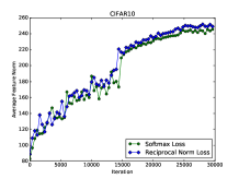
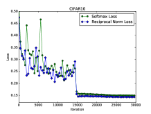
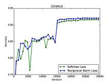
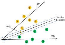
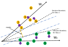
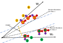
Figure 1: Comparison of softmax loss with softmax loss + feature incay(i.e., Reciprocal Norm Loss) on CIFAR10, results are showed in subfigure (a)(b)(c). (a) Average $\emph{L}_{2}$-norm of feature vectors versus iterations on test set, (b) softmax loss versus iterations on test set, (c) top-1 accuracy versus iterations on test set. In (d)(e)(f), we schematically illustrate different losses using binary classification as example, where yellow points are samples of class1 and green points are samples of class2. The black dashed line represents the decision boundary between the two classes. The two blue dashed lines represent the hyperplanes that pass the points with minimal distances to the decision boundary. The numbers 1-6 represent the increasing $\emph{L}_{2}$-norm of the points within each class. Their weight vectors within the softmax loss are $W_{1}$ and ${W_{2}}.$ (d) Feature embedding of softmax loss. (e) Feature embedding of large-margin softmax loss. The purple arrows represent the further constraints from large-margin softmax loss. Please refer  [11] for the detailed explanation about the two black dashed lines named Decision Boundary for Class1/Class2. (f) large-margin softmax loss + feature incay. The red arrows in (f) correspond to the loss constraints of feature incay. The margin between two classes increases from left to right by optimizing both the angles and $\emph{L}_{2}$-norm.

Deep Neural Networks (DNNs) with softmax loss have achieved state-of-the-art performance on various multi-class classification tasks. In DNNs, both representation and classifier are learned simultaneously in a single network, where the final representation for a sample is the feature vector $\mathbb{f}$ outputted from the penultimate layer, while the last layer outputs scores $z_{i}=\mathbb{w}_{i}\cdot\mathbb{f}$ for each category $i$, where $\mathbb{w}_{i}$ is the weight vector for category $i$. To define softmax loss, the scores are further normalized into probabilities via softmax function, i.e., $p_{i}=\frac{e^{z_{i}}}{\sum_{j}e^{z_{j}}}$. A well-trained DNN should output highest probability for the correct label in both training and testing phases, which requires the score for the correct label is significantly larger than other labels. Since $z_{i}=\mathbb{w}_{i}\cdot\mathbb{f}=\|\mathbb{w}\|\|\mathbb{f}\|\cos(\theta)$, where $\theta$ is the angle between $\mathbb{w}$ and $\mathbb{f}$, the goal of significant larger score for the correct label than other labels can be achieved by tuning $\|\mathbb{w}\|$, $\|\mathbb{f}\|$ and $\theta$. While increasing the weight norm $\|\mathbb{w}\|$ is constrained by weight decay for regularization, then $\|\mathbb{f}\|$ and $\theta$ become the two main factors for optimization. Softmax loss optimizes both factors but leaves much room to improve of each factor.

To improve softmax loss, large-margin softmax [11] is proposed to further decrease the angle between the feature vector and the weight vector of the correct label by adding more rigid constraint on the angle. Motivated by the fact that $\emph{L}_{2}$-normalized feature vector often results in better distance metric for retrieval tasks,  [16, 10] propose to use $\emph{L}_{2}$-normalized feature vector in softmax loss. Since feature vectors are normalized, feature norm has no affect on the score and only angle is optimized, which also results in much lower intra-class angular variability compared with softmax loss. All these methods explicitly or implicitly optimize the angle further but ignore the effect of feature norm. In this paper, feature incay is proposed to further optimize the factor of feature norm. In contrast to weight decay that favors weight vectors with small norm, feature incay favors feature vectors with large norm. From the computational perspective, larger feature norm results in larger score differences among categories, which can better separate the categories. From the perspective of pattern detection, larger feature norm encourages model to learn and detect more prominent patterns.

Feature incay is a general regularizer and can be added to softmax loss to emphasize feature norm. Whereas large-margin softmax emphasizes on the angle, feature incay can also be added to it to also emphasize on the feature norm. Specifically, feature incay is implemented by Reciprocal Norm Loss which minimizes the reciprocal of feature vectors’ $\emph{L}_{2}$ norm.

Figure 1, 1 and  1 shows the empirical results by adding feature incay to softmax loss, where feature incay brings larger $\emph{L}_{2}$-norm, smaller training loss and higher accuracy on test set. The geometric interpretation of feature incay is illustrated in Figure  1,  1 and  1, large-margin softmax 1 adds stronger constrain to align feature vectors to the weight vectors of their corresponding labels, by further adding feature incay 1, feature vectors are pushed away from the origin which results in better inter-class separability. Besides, Reciprocal Norm Loss is designed to increase the $\emph{L}_{2}$-norm adaptively according to the features’ original $\emph{L}_{2}$-norm, which can also help reduce the intra-class variances as illustrated in Figure  3.

In summary, we analyze the effect of the features’ $\emph{L}_{2}$-norm and prove (1) the benefit of the features’ $\emph{L}_{2}$-norm, (2) why the softmax loss fails to optimize the $\emph{L}_{2}$-norm of the features that have been well classified and (3) how our method can ensure the inter-class separability and intra-class compactness. The proposed Reciprocal Norm Loss is verified on three widely used classification datasets, i.e., MNIST, CIFAR10 and CIFAR100 using various network structures. We also propose the General Reciprocal Norm Loss to replace the softmax loss with other loss functions, such as Center loss and large-margin softmax loss. By considering the feature incay, we have achieved state-of-the-art performance on CIFAR10 and CIFAR100.

2 Related work

Large-margin Softmax Loss. Liu et al. [11] proposed to improve softmax loss by incorporating a adjustable margin $m$ multiplying the angle between a feature vector and the corresponding weight vector. Compared with the softmax loss, the new loss function pays more attention to the angular decision margin between classes as illustrated in Figure 1. Large-margin softmax loss adding stronger constrain to the angular, while feature incay adding stronger constrain to feature norm which is orthogonal to large-margin softmax loss as illustrated in Figure  1.

Center Loss. Wen et al. [17] proposed the center loss to learn centers for deep features of each class and penalize the distances between the deep features and their corresponding class centers. The softmax loss tries to align features vectors close to the weight vectors based on the inner product similarity, while center loss pushes feature vectors towards their class centers according Euclidean distances. Combining softmax loss with center loss actually uses two sets of classifiers, where representation is learned based on both the inner product to weight vector and the Euclidean distance to class center. The added center loss helps minimize the intra-class distances also by influencing the $\emph{L}_{2}$-norm of feature vectors, namely, small $\emph{L}_{2}$-norm will be increased and large $\emph{L}_{2}$-norm will be decreased along the process of pushing feature vectors to class centers. Different from center loss, feature incay also increases the norm of feature vectors with large $\emph{L}_{2}$-norm instead of penalizing feature vectors with large norm as center loss.

Weight/Feature Normalization. Inspired by the fact that feature normalization before calculating the sample distance usually achieves better performance for retrieval tasks, Rajeev et al. [13] proposed to use normalized feature vectors in softmax loss during training stage, thus the feature norm has no effect on softmax loss and angle is the main factor to be optimized. Congenerous cosine loss [12], NormFace [16], and cosine normalization [1] take a step further to normalize the weight vectors which replace inner product with cosine similarity within softmax loss, and only optimize the factor of angle. There normalization methods achieve much lower intra-class angular variability by emphasizing more on the angle during training, while ignore that feature norm is another useful factor worth to optimize.

3 Our work

3.1 Formulation of softmax loss

Let $\mathbb{X}=\{(x_{i},y_{i})\}_{i=1}^{N}$ be the training set contains $N$ samples, where $x_{i}$ is the raw input to the DNN, $y_{i}\in\{1,2,\cdots,K\}$ is the class label that supervises the output of the DNN. Denote $\mathbb{f}_{i}$ as the feature vector for $x_{i}$ learned by the DNN, $\{\mathbb{w}_{j}\}_{j=1}^{K}$ represent weight vectors for the $K$ categories. Then, softmax loss is defined as,

$$\mathcal{L}_{\text{softmax}}=-\frac{1}{N}\sum_{i=1}^{N}\log\bigg{(}\frac{e^{\mathbb{w}_{y_{i}}^{T}\mathbb{f}_{i}+\mathbb{b}_{y_{i}}}}{\sum_{j=1}^{K}e^{\mathbb{w}_{j}^{T}\mathbb{f}_{i}+\mathbb{b}_{j}}}\bigg{)}.$$ (1)

The bias term will be removed as it has been proven unnecessary in the recent works [11, 16]. Denote the angle between $\mathbb{w}_{j}$ and $\mathbb{f}_{i}$ as ${\theta}_{\mathbb{w}_{j},\mathbb{f}_{i}}$, the inner product between $\mathbb{w}_{j}$ and $\mathbb{f}_{i}$ can be rewritten as

$$\mathbb{w}_{j}^{T}\mathbb{f}_{i}=\|\mathbb{w}_{j}\|\|{\mathbb{f}_{i}}\|\cos({\theta}_{\mathbb{w}_{j},\mathbb{f}_{i}}).$$ (2)

By combining the above two equations, we get

$$\mathcal{L}_{\text{softmax}}=-\frac{1}{N}\sum_{i=1}^{N}\log\bigg{(}\frac{e^{\|\mathbb{w}_{y_{i}}\|\|\mathbb{f}_{i}\|\cos({\theta}_{\mathbb{w}_{y_{i}},\mathbb{f}_{i}})}}{\sum_{j=1}^{K}e^{\|\mathbb{w}_{j}\|\|\mathbb{f}_{i}\|\cos({\theta}_{\mathbb{w}_{j},\mathbb{f}_{i}})}}\bigg{)}$$ (3)

3.2 Properties of feature norm $\|\mathbb{f}_{i}\|$

Here are some properties that state why feature norm matters and why there is still improvement room for softmax loss. Before introducing these properties, we first introduce a Lemma that was proposed by [13]:

Lemma When the number of classes $K$ is smaller than twice the feature dimension $D$, we can distribute the classes on a hypersphere of dimenstion $D$ such that any two class weight vectors are at least $90^{\circ}$ apart.

The first property is similar to the proposition proved by [16], which states the relation between feature norm and softmax loss.

Property 1 By fixing weight vectors and directions of the feature vectors, softmax loss is a monotonically decreasing function with the increasing of the features’ $\emph{L}_{2}$-norm as long as the features are correctly classified.

Proof. Let $\mathcal{L}_{\text{softmax}}(\mathbb{f}_{i})$ represent the loss of the $i$-th sample, $i=1,\cdots,N$. Specifically,

$$\mathcal{L}_{\text{softmax}}(\mathbb{f}_{i}) =-\log\bigg{(}\frac{e^{\|\mathbb{w}_{y_{i}}\|\|\mathbb{f}_{i}\|\cos({\theta}_{\mathbb{w}_{y_{i}},\mathbb{f}_{i}})}}{\sum_{j=1}^{K}e^{\|\mathbb{w}_{j}\|\|\mathbb{f}_{i}\|\cos({\theta}_{\mathbb{w}_{j},\mathbb{f}_{i}})}}\bigg{)}$$

$$=-\log\bigg{(}\frac{1}{\sum_{j=1}^{K}e^{\|\mathbb{w}_{j}\|\|\mathbb{f}_{i}\|\cos({\theta}_{\mathbb{w}_{j},\mathbb{f}_{i}})-\|\mathbb{w}_{y_{i}}\|\|\mathbb{f}_{i}\|\cos({\theta}_{\mathbb{w}_{y_{i}},\mathbb{f}_{i}})}}\bigg{)}$$ (4)

Recall that when $\mathbb{f}_{i}$ is correctly classified, we have $\mathbb{w}_{y_{i}}^{T}\mathbb{f}_{i}>\mathbb{w}_{j}^{T}\mathbb{f}_{i}$ for any $j\neq y_{i}$, and $\|\mathbb{w}_{j}\|\|\mathbb{f}_{i}\|\cos({\theta}_{\mathbb{w}_{j},\mathbb{f}_{i}})-\|\mathbb{w}_{y_{i}}\|\|\mathbb{f}_{i}\|\cos({\theta}_{\mathbb{w}_{y_{i}},\mathbb{f}_{i}})\leq 0$ always holds. Then, for any $t>0$, we have

$$\mathcal{L}_{\text{softmax}}((1+t)\mathbb{f}_{i})<\mathcal{L}_{\text{softmax}}(\mathbb{f}_{i}),$$ (5)

which means increasing the norm of correctly classified samples can decrease the softmax loss. To consider all samples including incorrectly classified ones, we set $t_{i}>0$ if $i$ is correctly classified and $t_{i}=0$ otherwise, then we have

$$\sum_{i=1}^{N}\mathcal{L}_{\text{softmax}}((1+t_{i})\mathbb{f}_{i})\leq\sum_{i=1}^{N}\mathcal{L}_{\text{softmax}}(\mathbb{f}_{i})$$ (6)

So feature norm is an important factor to achieve smaller softmax loss together with the angle. $\hfill{}\Box$

Though the first property states that minimizing softmax loss encourages feature vectors towards large norm, there is still improvement room to achieve larger norm.

Property 2 For any feature vector $\mathbb{f}_{i}$, when the probability $P_{y_{i}}$ of the right category $y_{i}$ outputted by softmax function for $\mathbb{f}_{i}$ is close to one, the gradient of $\mathbb{f}_{i}$ computed based on softmax loss will be close to zero, which leads that the intra-class compactness and inter-class separability could not be further improved.

Proof. According to definition of softmax loss in Eq.(3), the gradient of feature vector $\mathbb{f}_{i}$ is:

$$\frac{\partial\mathcal{L}_{\text{softmax}}}{\partial\mathbb{f}_{i}}=\frac{1}{N}(-\mathbb{w}_{y_{i}}+\sum_{j=1}^{K}P_{j}\mathbb{w}_{j})$$ (7)

where the $P_{j}=\frac{e^{\mathbb{w}_{j}^{T}\mathbb{f}_{i}}}{\sum_{j=1}^{K}e^{\mathbb{w}_{j}^{T}\mathbb{f}_{i}}}$. When $P_{y_{i}}\to 1$ and $P_{j}\to 0(\forall j\neq y_{i})$, $\frac{\partial\mathcal{L}_{\text{softmax}}}{\partial\mathbb{f}_{i}}\to 0$. That is after a training sample is confidently classified correctly, it will have no contribution to its own representation learning. For example, suppose $\|\mathbb{w}_{j}\|=1$, ${\theta}_{\mathbb{w}_{y_{i}},\mathbb{f}_{i}}=0$ and ${\theta}_{\mathbb{w}_{j},\mathbb{f}_{i}}\geq 90^{\circ}(\forall j\neq y_{i})$ according the Lemma, then $\|\mathbb{w}_{y_{i}}\|\|\mathbb{f}_{i}\|\cos({\theta}_{\mathbb{w}_{y_{i}},\mathbb{f}_{i}})=\|\mathbb{f}_{i}\|$, $\|\mathbb{w}_{j}\|\|\mathbb{f}_{i}\|\cos({\theta}_{\mathbb{w}_{j},\mathbb{f}_{i}})<0,\forall j\neq y_{i}$. Putting together, we have $P_{y_{i}}\geq\frac{e^{\|\mathbb{f}_{i}\|}}{e^{\|\mathbb{f}_{i}\|}+K-1}$, for a modest number of categories say $K=10$, $P_{y_{i}}>0.999$ when $\|\mathbb{f}_{i}\|=10$. More categories can optimize to larger feature norm before softmax is saturation.

$\hfill{}\Box$

This property says feature norm can still be elongated even the softmax loss is 0. The Reciprocal Norm Loss discussed in next section is to further elongate the feature norm explictly.

3.3 Reciprocal Norm Loss

Reciprocal Norm Loss adds a term of feature incay to penalize feature vectors with small norm and formally defined as

$$\quad\mathcal{L}=\underbrace{-\frac{1}{N}\sum_{i=1}^{N}\log\bigg{(}\frac{e^{\mathbb{w}_{y_{i}}^{T}\mathbb{f}_{i}}}{\sum_{j=1}^{K}e^{\mathbb{w}_{j}^{T}\mathbb{f}_{i}}}\bigg{)}}_{\text{softmax loss}}+\underbrace{\mu\sum_{k=1}^{K}\|\mathbb{w}_{k}\|^{2}}_{\text{weight decay}}+\underbrace{\lambda\frac{1}{N}\sum_{i=1}^{N}\frac{h(i)}{\|\mathbb{f}_{i}\|^{2}+\epsilon}}_{\text{feature incay}}$$ (8)

where the $h(i)$ is an indicator function, and $h(i)=1$ when the $\mathbb{f}_{i}$ is correctly classified otherwise $h(i)=0$, $\epsilon$ is a small positive value to prevent dividing by value close to zero, $\lambda$ is a hyperparameter used to control the influence of feature incay. The whole loss function consists of three parts: softmax loss, weight decay and feature incay, and together they favor weights that achieve small softmax loss, small weight norm and large feature norm. In the early stage of training, most $h(i)$ are equal to 0, and softmax loss and weight decay are active in training, and feature incay is gradually adding in along with training to reinforce the feature vectors that result in correct classification. Large feature norm brings large inter-class separability under the constrain of small weight norm, otherwise large feature norm can be trivially achieved by increasing the weight norm. The simple reciprocal form of feature norm has another nice property that moves feature vectors with small norm fast while moves feature vectors with large norm slow, which results intra-class compactness. Specifically, denote feature incay of $\mathbb{f}_{i}$ as $\mathcal{F}(\mathbb{f}_{i})=\frac{h(i)}{\|\mathbb{f}_{i}\|^{2}+\epsilon}$, when $h(i)=1$, the gradient is $\frac{\partial\mathcal{F}}{\partial\mathbb{f}_{i}}=-\frac{2\mathbb{f}_{i}}{(\|\mathbb{f}_{i}\|^{2}+\epsilon)^{2}}$. For any two feature vectors $\mathbb{f}_{p}$ and $\mathbb{f}_{q}$ satisfying $\|\mathbb{f}_{q}\|\hskip 2.84526pt>\|\mathbb{f}_{p}\|$, we always have $\|\frac{\partial\mathcal{F}}{\partial\mathbb{f}_{p}}\|\hskip 2.84526pt>\|\frac{\partial\mathcal{F}}{\partial\mathbb{f}_{q}}\|$. That is feature vectors with small norm increase fast along their original directions while feature vectors with large norm increase slowly along their original directions.

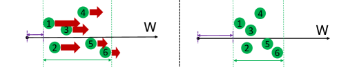
Figure 2: The original data distribution is on the left of the black dashed line and the data distribution updated according to the Reciprocal Norm Loss is on the right. The numbers 1-6 represent the points are of increasing feature norm. The black point represents the original point. The lengthes of the green bidirectional arrows represent the maximal distance in the direction of the weight vectors within all the points of one class. The purple bidirectional arrow means the minimal distance to origin, which is equal to the minimal feature norm. The red arrows represent the gradients update along the directions of the weight vectors computed with the Reciprocal Norm Loss, while the length represents the size of the gradient.

3.4 Geometric Interpretation of Reciprocal Norm Loss

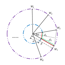
Figure 3: Illustration in 2-dimensional space.

Property 3 Suppose (a) the angle between any feature vector $\mathbb{f}_{i}$ and its corresponding weight vector $\mathbb{w}_{y_{i}}$ is zero, (b) the angles between any two neighbor weight vectors of different classes are $\theta$, we have (1) the minimal inter-class distance is $2\alpha\sin(\frac{\theta}{2})$, where $r$ is lower bound of feature norm, (2) when $K<2D$, the upper bound of feature norm is in the range of $[(1+\sqrt{2})\alpha,3\alpha]$ to ensure the maximal intra-class distance is smaller than the minimal inter-class distance.

Proof. Figure 3 shows the 2-dimensional case satisfying the conditions(a)(b), where black arrows named with $W_{i}$ represent weight vectors for each class. As we have assumed all feature vectors are lying on the directions of their corresponding $W_{i}$, and blue circle and purple circle denote the lower bound and upper bound of feature norm respectively. Thus the maximal intra-class distance is $d_{2}=\beta-\alpha$ and the minimal inter-class distance is $d_{1}=2\alpha\sin(\frac{\theta}{2})$. To ensure minimal inter-class distance is larger than intra-class distance, i.e., $d_{1}=2\alpha\sin(\frac{\theta}{2})>d_{2}=\beta-\alpha$, which requires $\beta<2\alpha\sin(\frac{\theta}{2})+\alpha$.

When $K<2D$, according to the Lemma, we can ensure that $\theta\geq 90^{\circ}$. Besides, the angle between any two vectors is smaller than $180^{\circ}$. Then $\frac{\theta}{2}\in[45^{\circ},90^{\circ}]$ and $\sin(\frac{\theta}{2})$ is a monotonously increasing function within the range $[45^{\circ},90^{\circ}]$. Based on $\sin(\frac{\theta}{2})\in[\frac{\sqrt{2}}{2},1]$, the upper bound of $\emph{L}_{2}$-norm of feature vectors is in the range $[(1+\sqrt{2})\alpha,3\alpha]$.

$\hfill{}\Box$

According to the Property, the feature norm does not need to increase endlessly, which can also be achieved by feature incay since feature vectors with large norm have negligible effect on the model. we can estimate an upper bound according to the original features’ $\emph{L}_{2}$-norm. In our experiments, we will choose the average $\emph{L}_{2}$-norm as the lower bound to avoid the outlier.

In summary, besides information in training examples and complexity of the neural network [5], feature norm can also influence the generalization ability.

4 Experiments

In this section, we verify the effectiveness of feature incay through empirical experiments.

4.1 Experimental Settings

We evaluate feature incay on three datasets, i.e., MNIST, CIFAR10, and CIFAR100. MNIST consists of 60,000 training images and 10,000 test images from 10 handwritten digits, both CIFAR10 and CIFAR100 contain 50,000 training images and 10,000 test images from 10 object categories and 100 object categories respectively. Images are horizontally flipped randomly and subtracted by mean image. Neural networks architectures used in [11] are adopt with minor modification as detailed in Table  1, and implemented based on Caffe framework [4]. The weight $\mu$ for weight decay is 0.0005, the weight $\lambda$ is set with different values in different experiments, e.g., 1.0, 0.1 or 0.01. The momentum is 0.9, and the learning rate starts from 0.1 and divided by a factor of 10 three times when the training error stops decreasing.

Table 1: The CNN architectures used for MNIST/CIFAR10/CIFAR100. The count of the Conv1.x, Conv2.x and Conv3.x closely follows the settings in  [11]. All the pooling layers are with window size $2\times 2$ and stride of 2.

Layer	MNIST-2D	MNIST	CIFAR10	CIFAR100
Conv0.x	$[5\times 5,20]\times 1$	$[3\times 3,64]\times 1$	$[3\times 3,64]\times 1$	$[3\times 3,128]\times 1$
Conv1.x	$[5\times 5,50]\times 1$	$[3\times 3,64]\times 3$	$[3\times 3,64]\times 4$	$[3\times 3,128]\times 4$
Conv2.x	N/A	$[3\times 3,64]\times 3$	$[3\times 3,128]\times 4$	$[3\times 3,256]\times 4$
Conv3.x	N/A	$[3\times 3,64]\times 3$	$[3\times 3,256]\times 4$	$[3\times 3,512]\times 4$
Fully Connected	2	256	512	512

Table 2: Results on MNIST.

Method	Accuracy	Average $\emph{L}_{2}$-norm
Softmax	88.62	316.65
RN + Softmax	89.44	488.86
L-Softmax	89.91	329.92
RN + L-Softmax	92.06	552.54
Center Loss	89.01	192.15
RN + Center Loss	91.32	273.78

4.2 Quick Experiments

To quickly evaluate the effectiveness of feature incay, we experiment on MNIST using a very simple neural network with only two convolutional layers as listed in Table 1. Due the simplicity of the model and the task, the training error can be converged in only 10,000 iterations. Table 2 summarizes the top-1 accuracy and average $\emph{L}_{2}$-norm on test set by using Softmax, large-margin Softmax (L-Softmax), Softmax with center loss (Center Loss), and with feature incay (RN+). L-Softmax, Center Loss and RN+Softmax improve Softmax, and RN+L-Softmax and RN+Center Loss improve L-Softmax and Center Loss further. With explicitly penalizing feature vectors with small norm, feature incay significantly increases the average feature norm as expected.

4.3 Comparison Experiments

To achieve state-of-the-art performance on the three datasets, we use deep neural networks as specified in last three columns. Feature incay is added to Sofmax and L-Softmax to compare with state-of-the-art approaches, and the reproduced results by Softmax and L-Softmax following [11] are slightly better than the referred numbers in general. Table 3 lists the error rates of compared approaches and our method. In can be concluded that feature incay can consistently improve over Softmax, and improves L-Softmax on CIFAR10 and CIFAR100, while slightly worse than our reproduced L-Softmax on MNIST, we hypothesis that the performance on MNIST is already saturate and difficult to improve further.

Table 3: Error rate (%) on MNIST/CIFAR10/CIFAR100

Method	MNIST	CIFAR10	CIFAR100
CNN [3]	0.53	N/A	N/A
DropConnect [15]	0.57	9.41	N/A
FitNet [14]	0.51	N/A	35.04
NiN [9]	0.47	10.47	35.68
Maxout [2]	0.45	11.68	38.57
DSN [7]	0.39	9.69	34.57
R-CNN [8]	0.31	8.69	31.75
GenPool [6]	0.31	7.62	32.37
Hinge Loss [11]	0.47	9.91	33.10
Softmax [11]	0.40	9.05	32.74
L-Softmax [11]	0.31	7.58	29.53
Softmax	0.35	8.45	32.36
RN + Softmax	0.31	7.96	31.76
L-Softmax	0.25	7.55	29.95
RN + L-Softmax	0.29	7.32	29.18

Figure 4, 4 and 4 show the accuracy, average feature norm and softmax loss during training by using $\lambda=1,0.1,0.01$ respectively. Feature incay achieves better or comparable accuracy compared with softmax loss under a wide range of $\lambda$, and results in larger feature norm on both training and test set. All methods achieve close to zero softmax loss on training set, while feature incay ensures lower softmax loss on test set. Figure 4 shows the accuracy versus iteration number on CIFAR100, which is similar to the results on CIFAR10.

4.4 Effects of $\lambda$

Table 4: Accuracy(%) Comparison of different $\lambda$

Method	$\lambda=0$	$\lambda=1$	$\lambda=0.1$	$\lambda=0.01$
RN + Softmax	91.55	91.68	92.04	91.96
RN + L-Softmax	92.45	92.36	92.38	92.68

We conduct experiments on CIFAR10 to investigate how to choose the hyperparamter $\lambda$. Results are show in Table 4. Softmax loss with feature incay achieves consistent improvement for all the different choices of $\lambda$. For adding feature incay to L-Softmax, only small $\lambda$ could improve the performance. This is due to L-Softmax emphasize more on the angle and often results in smaller feature norm than softmax loss, and the feature incay will be much larger, to balance the L-Softmax loss and feature incay for training, $\lambda$ should be set to a relatively small number.

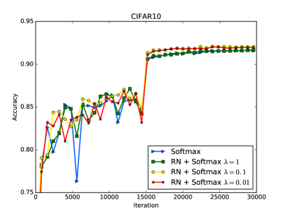
a

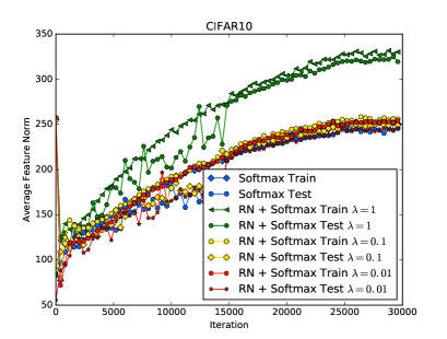
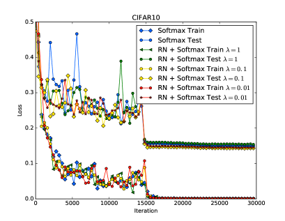
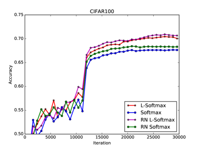
Figure 4: (a) Accuracy versus iterations with different choices of $\lambda$ value on the test set of CIFAR10. The RN Softmax achieves 92.04% when $\lambda=0.1$ (b) The training/testing sets’ $\emph{L}_{2}$ norm versus iterations with different choices of the $\lambda$ value on CIFAR10. The RN Softmax with different $\lambda$ all achieve larger $\emph{L}_{2}$-norm. (c) The training/testing sets’ loss vs. iterations with different choices of the $\lambda$ value on CIFAR10. The RN Softmax achieves notable smaller loss value 0.1432 than the Softmax with 0.1498. (d) Accuracy vs. iterations with Softmax/RN Softmax/L-Softmax/RN L-Softmax on CIFAR100.

5 Conclusions and future work

In this paper, we propose a novel Reciprocal Norm Loss as a new kind of regularizer named feature incay considering feature vectors are also tunable in DNNs. Feature incay reinforces feature vectors that result in correct classification, and elongate feature vectors with small norm fast than feature vectors with large norm, thus can decrease intra-class distance and increase inter-class distance at the same time. We also give the theoretical proof of why the feature norm matters, why there is still improvement room for the widely used softmax loss. Extensive experiments on MNIST, CIFAR10 and CIFAR100 verify the effectiveness of our method. In the future work, we plan to investigate other substitute feature incay and mine the inner relations between the feature incay and the weight decay.

References

- [1] Luo Chunjie, Yang Qiang, et al. Cosine normalization: Using cosine similarity instead of dot product in neural networks. arXiv preprint arXiv:1702.05870, 2017.
- [2] Ian J Goodfellow, David Warde-Farley, Mehdi Mirza, Aaron Courville, and Yoshua Bengio. Maxout networks. arXiv preprint arXiv:1302.4389, 2013.
- [3] Kevin Jarrett, Koray Kavukcuoglu, Yann LeCun, et al. What is the best multi-stage architecture for object recognition? In Computer Vision, 2009 IEEE 12th International Conference on, pages 2146–2153. IEEE, 2009.
- [4] Yangqing Jia, Evan Shelhamer, Jeff Donahue, Sergey Karayev, Jonathan Long, Ross Girshick, Sergio Guadarrama, and Trevor Darrell. Caffe: Convolutional architecture for fast feature embedding. In Proceedings of the 22nd ACM international conference on Multimedia, pages 675–678. ACM, 2014.
- [5] Anders Krogh and John A Hertz. A simple weight decay can improve generalization. In Advances in neural information processing systems, pages 950–957, 1992.
- [6] Chen-Yu Lee, Patrick W Gallagher, and Zhuowen Tu. Generalizing pooling functions in convolutional neural networks: Mixed, gated, and tree. In International conference on artificial intelligence and statistics, 2016.
- [7] Chen-Yu Lee, Saining Xie, Patrick Gallagher, Zhengyou Zhang, and Zhuowen Tu. Deeply-supervised nets. In Artificial Intelligence and Statistics, pages 562–570, 2015.
- [8] Ming Liang and Xiaolin Hu. Recurrent convolutional neural network for object recognition. In Proceedings of the IEEE Conference on Computer Vision and Pattern Recognition, pages 3367–3375, 2015.
- [9] Min Lin, Qiang Chen, and Shuicheng Yan. Network in network. arXiv preprint arXiv:1312.4400, 2013.
- [10] Weiyang Liu, Yandong Wen, Zhiding Yu, Ming Li, Bhiksha Raj, and Le Song. Sphereface: Deep hypersphere embedding for face recognition. arXiv preprint arXiv:1704.08063, 2017.
- [11] Weiyang Liu, Yandong Wen, Zhiding Yu, and Meng Yang. Large-margin softmax loss for convolutional neural networks. In Proceedings of The 33rd International Conference on Machine Learning, pages 507–516, 2016.
- [12] Yu Liu, Hongyang Li, and Xiaogang Wang. Learning deep features via congenerous cosine loss for person recognition. arXiv preprint arXiv:1702.06890, 2017.
- [13] Rajeev Ranjan, Carlos D Castillo, and Rama Chellappa. L2-constrained softmax loss for discriminative face verification. arXiv preprint arXiv:1703.09507, 2017.
- [14] Adriana Romero, Nicolas Ballas, Samira Ebrahimi Kahou, Antoine Chassang, Carlo Gatta, and Yoshua Bengio. Fitnets: Hints for thin deep nets. arXiv preprint arXiv:1412.6550, 2014.
- [15] Li Wan, Matthew Zeiler, Sixin Zhang, Yann L Cun, and Rob Fergus. Regularization of neural networks using dropconnect. In Proceedings of the 30th International Conference on Machine Learning (ICML-13), pages 1058–1066, 2013.
- [16] Feng Wang, Xiang Xiang, Jian Cheng, and Alan L Yuille. Normface: hypersphere embedding for face verification. arXiv preprint arXiv:1704.06369, 2017.
- [17] Yandong Wen, Kaipeng Zhang, Zhifeng Li, and Yu Qiao. A discriminative feature learning approach for deep face recognition. In European Conference on Computer Vision, pages 499–515. Springer, 2016.