Bifurcation of traveling waves in a Keller-Segel type free boundary model of cell motility

Abstract

We study a two-dimensional free boundary problem that models motility of eukaryotic cells on substrates. This problem consists of an elliptic equation describing the flow of cytoskeleton gel coupled with a convection-diffusion PDE for the density of myosin motors. The two key properties of this problem are (i) presence of the cross diffusion as in the classical Keller-Segel problem in chemotaxis and (ii) nonlinear nonlocal free boundary condition that involves curvature of the boundary. We establish the bifurcation of the traveling waves from a family of radially symmetric steady states. The traveling waves describe persistent motion without external cues or stimuli which is a signature of cell motility. We also prove existence of non-radial steady states. Existence of both traveling waves and non-radial steady states is established via Leray-Schauder degree theory applied to a Liouville-type equation (which is obtained via a reduction of the original system) in a free boundary setting.

1 Introduction

For decades, the persistent motion exhibited by keratocytes on flat surfaces has attracted attention from experimentalists and modelers alike. Cells of this type are found, e.g., in the cornea and their movement is of medical relevance as they are involved in wound healing after eye surgery or injuries. Also, keratocytes are perfect for experiments and modeling since they naturally live on flat surfaces, which allows capturing the main features of their motion by spatially two dimensional models. The typical modes of motion of keratocytes are rest (no movement at all) or steady motion with fixed shape, speed, and direction. That is why the most important solutions will be steady state solutions (corresponding to a resting cell) and traveling wave solutions (a steadily moving cell).

Traveling wave solutions for cell motility models have been investigated both analytically and numerically for free boundary problems in one space dimension, e.g. [36, 37, 2], numerically for free boundary models in two dimensions, e.g. [3, 42], as well as for phase field models, analytically in one dimension, e.g. [5], and numerically in two dimensions, e.g. [40, 47, 39], for an overview we refer to [46, 1] and references therein. In this work we consider a two-dimensional model that can be viewed both as an extension of the analytical one-dimensional model from [36, 37] to 2D and as a simplified version of the computational 2D model from [3]. Our objective is to study the existence of traveling wave solutions for this model. These solutions describe steady motion without external cues or stimuli which is a signature of cell motility.

In [36, 37], the authors introduced a one dimensional model capturing actin (more precisely, filamentous actin or F-actin) flow and contraction due to myosin motors. They proposed a model that consists of a system of an elliptic and a parabolic equation of Keller-Segel type in the free boundary setting. It was shown in [36] that trivial steady states bifurcate to traveling wave solutions. The Keller-Segel system in fixed domains was first introduced and analyzed in [21, 22, 23] and studied by many authors due to its fundamental importance in biology most notably for modeling chemotaxis. There is a vast body of literature on Keller-Segel models with prescribed (fixed rather than free) boundary, see, e.g., [35], [9],[43], [44] review [17] and references therein. The key issue in such problems is the blow up of the solutions depending on the initial data.

In [3] a two-dimensional free boundary model consisting of PDEs for actin flow, myosin density and, additionally, a reaction-diffusion equation for the cell-substrate adhesion strength was introduced based on mechanical principles. Simulations of this model reveal steady state and traveling wave type solutions in two-dimensions that are compared to experimental observations of keratocyte motion on the flat surfaces. The steady state solutions are characterized by a high adhesion strength (high traction) whereas the moving cell solutions correspond to a low overall adhesion strength. In both cases, the adhesion strength is spatially almost homogeneous. Therefore in this work we consider a simplified two-dimensional problem with constant adhesion strength parameter similar to the one dimensional model of [36, 37]. We further simplify the model in [3], see also review [38] by considering a reduced rheology of the cytoskeleton based on the high contrast in numerical values for shear and bulk viscosities cited in [3]. Thus following [32] we consider equations $[S1]-[S2]$ from [3] with shear viscosity $\mu=0$ and bulk viscosity $\mu_{b}$ scaled to $1$.

The main building block of the model considered in this work is a coupled Keller-Segel type system of two partial differential equations. The first one (obtained after the above simplification of equation $[S1]$ from [3]) in dimension-free variables writes as follows:

$$\nabla\,{\rm div}\,u+\alpha\nabla m=u\quad\mbox{in }\Omega(t),~{}~{}~{}~{}~{}~{}$$ (1.1)

where $\Omega(t)$ is the time dependent domain in $\mathbb{R}^{2}$ occupied by the cell, $u$ is the velocity of the actin gel, and $m$ is the myosin density. This equation represents the force balance between the stress in the actin gel on the left hand side and the friction (proportional to the velocity) between the cell and the substrate on the right hand side. Since the shear viscosity $\mu=0$, the stress $S$ is a scalar composed of a hydrodynamic (passive) part $\mathrm{div}\,u$ and the active contribution $\alpha m$ generated by myosin motors. Identifying $S$ with the corresponding scalar matrix (tensor $S\mathbb{I}$), equation (1.1) can be rewritten in the standard form ${\rm div}S=u$. Equation (1.1) is coupled to an advection-diffusion equation for the myosin density $m$:

$$\partial_{t}m=\Delta m-{\rm div}(u\,m)\quad\mbox{in }\Omega(t).$$ (1.2)

Myosin motors are transported with the actin flow if bound to actin and freely diffuse otherwise, reflected by the second and first term on the right hand side of (1.2), respectively. Assuming that the time scale for binding and unbinding is very short compared to those relevant for our problem, the densities of bound and unbound myosin motors can be combined into the effective density $m$ (see e.g. [36, 37]).

Following [3], the evolution of the free boundary $\partial\Omega(t)$ is described by the kinematic boundary condition for the normal velocity $V_{\nu}$,

$$V_{\nu}=(u\cdot\nu)-\beta\kappa+\lambda\quad\mbox{on }\partial\Omega(t),$$ (1.3)

where $\nu$ is the unit outward normal, $\kappa$ stands for the curvature of $\partial\Omega(t)$, and constant $\lambda$ defined by $\lambda:=\left(2\pi\beta-\int_{\partial\Omega(t)}(u\cdot\nu)d\sigma\right)/|\partial\Omega(t)|$ enforces area preservation. The kinematic condition (1.3) equates the normal velocity $V_{\nu}$ of the boundary to the contributions from the normal component $(u\cdot\nu)$ of the actin velocity, the surface tension $\beta\kappa$ of the membrane ($\kappa$ being the curvature), and the area preservation term $\lambda$. The latter term is constant along the boundary and is interpreted as actin polymerization at the membrane, it compensates for the difference between velocities of the actin gel and the membrane.

On the boundary, equation (1.1) is supplied with the zero stress condition

$${\rm div}u+\alpha m=0\ ~{}~{}\mbox{on }\partial\Omega(t).$$ (1.4)

whereas for the equation (1.2), a no-flux condition is assumed:

$$\frac{\partial m}{\partial\nu}=(u\cdot\nu)m\quad~{}~{}~{}\mbox{on }\partial\Omega(t).$$ (1.5)

Similar parabolic-elliptic free boundary problems frequently occur in modeling of biological and physical phenomena. One type of problem arises in tumor growth models, e.g. [13, 11, 16, 18] (see also reviews [12, 30]), however, these are typically linear problems, and the domain area is not preserved. For these models, steady state solutions have been described, and bifurcations to different steady states or growing/shrinking domain solutions have been investigated. Another type of problem arises in the modeling of wound healing, see, e.g., [19], where a free boundary problem for a reaction diffusion equation is used to model the evolution of complex wound morphologies. These models are often agent based rather than continuum models, see, e.g., [7]. More recently, mechanical tumor models have been devised leading to Hele-Shaw type problems, e.g. [34].

In the above works the focus is on solutions describing motion with constant velocity in domains that expand or contract rather than domains of fixed size and shape moving with constant velocity. Besides this shift of focus, the main novelty of the free boundary problem under consideration is the cross diffusion term in equation (1.2) giving rise to the Keller-Segel structure of the bulk equations. This structure was introduced in one dimensional models of cell motility in [36, 37]. While the boundary in one dimensional models (e.g. [36, 37]) consists of just two points, in two dimensional free boundary models the shape of the domain is unknown. This poses questions that do not arise in one dimensional settings and leads to novel challenges in analysis, for example, bifurcations from radially symmetric to non-radially symmetric shapes.

We are interested in traveling wave solutions of (1.1) - (1.3), i.e. solutions of the form $\Omega_{t}=\Omega+Vt$, $u=u(x-V_{x}t,y-V_{y}t)$, $m=m(x-V_{x}t,y-V_{y}t)$. Thus after passing to the moving frame and rewriting system (1.1)-(1.5) in terms of the scalar stress $S:={\rm div}u+\alpha m$ we are led to the following free boundary problem

$$-\Delta S+S=\alpha m\quad\mbox{in }\Omega,\ \mbox{and}\quad S=0\quad\mbox{on}\ \partial\Omega,$$ (1.6)

$$-\Delta m+{\rm div}((\nabla S-V)m)=0\quad\mbox{in }\Omega,\ \mbox{and}\quad\frac{\partial m}{\partial\nu}=((\nabla S-V)\cdot\nu)m\ \quad\mbox{on }\partial\Omega,$$ (1.7)

$$V_{\nu}=\frac{\partial S}{\partial\nu}-\beta\kappa+\lambda\quad\mbox{on }\partial\Omega.$$ (1.8)

We now outline the main result of the paper (see, Section 6 for further details) and key ingredients of the proof.

Theorem 1.1.

There is a family of traveling waves solutions of (1.6)-(1.8) with nonzero velocities $V$, bifurcating from radially symmetric steady state solutions. This family exists for all values of parameters $\alpha>0$ and $\beta>0$ (except, possibly, for a countable number of values of $\beta$, see Theorem 7.2) and for any domain area $|\Omega|$.

Without loss of generality we assume motion in $x$-direction and, slightly abusing notation, write $V=(V,0)$. Furthermore, for a given $S$ all nonnegative solutions of (1.7) ($m$ represents the density of myosin and therefore cannot be negative) are given by $m(x,y)=m_{0}e^{S(x,y)-xV}$ with some constant $m_{0}\geq 0$. Indeed, it is straightforward that $m=e^{S(x,y)-xV}$ is a solution of (1.7). The uniqueness up to a multiplicative constant follows from the Krein-Rutman theorem [26], or alternatively using the factorization $m=m_{0}(x,y)e^{S(x,y)-xV}$, considering $m_{0}$ as a unknown function, and proving that $m_{0}=\rm{const}$ by showing that it satisfies an advection-diffusion equation with zero Neumann condition. This allows us to eliminate $m$ from (1.6)-(1.7) and rewrite the problem of finding traveling waves in the following concise form:

$$-\Delta S+S=\Lambda e^{S-xV}\quad\mbox{in }\Omega,$$ (1.9)

with boundary conditions

$$S=0\quad\mbox{on }\partial\Omega$$ (1.10)

and

$$V\nu_{x}=\frac{\partial S}{\partial\nu}-\beta\kappa+\lambda\quad\mbox{on }\partial\Omega.$$ (1.11)

Note that an ODE similar to the PDE (1.9) was obtained in the analysis of the one dimensional free boundary problem for the Keller-Segel type system in [36, 37]. In problem (1.9)-(1.11) $S$, $V$, and $\Lambda=m_{0}\alpha\geq 0$ are unknowns and the parameter $\beta$ is given. Note that (1.9)-(1.11) is a free boundary problem, that is, the domain $\Omega$ is also unknown. For radially symmetric solutions of (1.9)-(1.10) with $V=0$ and $\Omega$ being a disk, the constant $\lambda$ can always be chosen so that the boundary condition (1.11) is satisfied. This observation allows us to construct a one-parameter family of radially symmetric steady state solutions by solving the nonlinear eigenvalue problem (1.9)-(1.10). Furthermore, the equation (1.9) contains exponential nonlinearity, as in the classical Liouville equation [29] which has explicit radially symmetric solutions, but the additional zero order term $S$ in the left hand side of (1.9) complicates the analysis. Note that non-trivial steady states also exist in the one-dimensional case [36, 37] (they are unstable).

We rely on an argument from [10] (see also [25]) based on the Implicit Function Theorem to show existence of an analytic curve $\mathcal{A}_{1}$ of radially symmetric solutions of (1.9)-(1.10). Moreover these solutions are extended to the case of nonzero $V$ in (1.9) and small perturbations of the domain $\Omega$ from a given disk. Then (1.9)-(1.11) is reduced to selecting solutions of (1.9)-(1.10) that satisfy (1.11). Considering the linear part of perturbations of radially symmetric solutions we (formally) derive the condition (3.8) (Section 3) for a bifurcation from the steady states to genuine traveling waves (with $V\not=0$). We next show that the condition (3.8) is indeed satisfied on a nontrivial radially symmetric steady state solution belonging to $\mathcal{A}_{1}$, exploiting a subtle bound on the second eigenvalue of the linearized problem for the Liouville equation from [41]. Yet another technically involved part of this work is devoted to recasting (1.9)-(1.11) as a fixed point problem in an appropriate functional setting. Then a topological argument based on Leray-Schauder degree theory rigorously justifies the existence of traveling waves with $V\not=0$. Both the recasting and the topological argument require spectral analysis of various linearized operators appearing in these considerations. Next the techniques developed for establishing traveling waves solutions are also used to find steady states with no radial symmetry.

The rest of paper is organized as follows. In Section 2 we find a one parameter family of radially symmetric steady state solutions and establish their properties. In Section 3 we derive a necessary condition (3.8) for the bifurcating from the family of radially symmetric steady states to a family of traveling wave solutions ($V\neq 0$) and show that this condition is satisfied on the analytic curve $\mathcal{A}_{1}$ of radially symmetric solutions. In Section 4 we investigate the spectral properties of the linearized operator of the equation (1.9) around radially symmetric steady states. This operator appears in a number of the subsequent constructions. In section 5 we establish existence of the solutions to the Dirichlet problem (1.9)-(1.10) and study their properties. This is done for small but not necessarily zero velocity $V$ in a prescribed domain $\Omega$, which is a perturbation of a disk. Section 6 completes the proof of the main result on the bifurcation of the steady states to traveling waves. To this end we rewrite (1.9)-(1.11) as a fixed point problem, and study the local Leray-Schauder index of the corresponding mapping. We show that this index jumps at the potential bifurcation point (identified in Section 3). This establishes the bifurcation at this point. Finally, in section 7 we prove existence of nonradial steady states. In the Appendix A we construct three terms of the asymptotic expansion of traveling wave solutions in powers of small velocity, which allow us to describe the emergence of non-symmetric shapes both analytically and numerically.

2 Family of radially symmetric steady states

Problem (1.9)-(1.11) has a family of steady solutions, with $V=0$, found in a radially symmetric form. Namely, let $\Omega$ be a disk $B_{R}$ with radius $R>0$, then we seek radially symmetric solutions $S=\Phi(r)$, $r=\sqrt{x^{2}+y^{2}}$, of the equation

$$-\frac{1}{r}(r\Phi^{\prime}(r))^{\prime}+\Phi=\Lambda e^{\Phi},\quad 0<r<R,$$ (2.1)

with boundary conditions

$$\Phi^{\prime}(0)=\Phi(R)=0.$$ (2.2)

Note that (2.1)-(2.2) is a nonlinear eigenvalue problem, i.e. both the constant $\Lambda$ and the function $\Phi(r)$ are unknowns in this problem. Every solution of (2.1)-(2.2) also satisfies (1.9)-(1.11) with $V=0$ and some constant $\lambda$, that is we can always choose $\lambda$ in this radially symmetric problem, so that the condition (1.11) is satisfied. Equation (2.1) is the classical Liouville equation [29] with an additional zero order term (the second term on the left hand side of (2.1)). Various forms of the Liouville equation arise in many applications ranging from the geometric problem of prescribed Gaussian curvature to the relativistic Chern-Simons-Higgs model [33], the mean field limit of point vortices of Euler flow [8] and the Keller-Segel model of chemotaxis [45]. For a review of the literature on Liouville type equations we address the reader to [28] and references therein. While the above works mostly address the issues related to the blow-up in the Liouville equation, see e.g., [27], in contrast our focus is on the construction of the family of solutions and its properties. Since we are concerned with special solutions of (1.1)-(1.5) such as traveling waves and steady states rather than general properties of this evolution problem, the issue of blow-up does not arise.

The following theorem establishes existence of solutions of problem (2.1)-(2.2), and the subsequent lemma lists some of their properties.

Remark 2.1.

It is natural to expect that the set of solutions of (2.1)-(2.2) has the same structure as the explicit solutions of the classical Liouville equation [41] in the disk. However, the presence of the additional term $S$ in (2.1) complicates the analysis even in the radially symmetric case, in particular, the standard trick based of Pohozhaev identity no longer can be used to establish non-degeneracy (see condition (2.8)).

Theorem 2.2.

Fix $R>0$, then

(i) There exists a continuum (a closed connected set) $\mathcal{K}\subset\mathbb{R}\times C([0,R])$ of nonnegative solutions $\Lambda\geq 0$, $\Phi\geq 0$ of (2.1)-(2.2), emanating from the trivial solution $(\Lambda,\Phi)=(0,0)$. There exists a finite positive

$$\Lambda_{0}=\max\{\Lambda\,|\,\text{\eqref{radialLiouville}-\eqref{radialLiouvilleBC} has a solution }(\Lambda,\Phi)\},$$

in particular, $\Lambda\leq\Lambda_{0}$ for all $(\Lambda,\Phi)\in\mathcal{K}$. On the other hand $\|\Phi\|_{C([0,R])}$ is not bounded in $\mathcal{K}$, and moreover

$$\sup\left\{\int_{0}^{R}e^{\Phi}\,rdr\,|\,(\Lambda,\Phi)\in\mathcal{K}\right\}=\infty.$$ (2.3)

(ii) For every $0\leq\Lambda<\Lambda_{0}$ there exists a pointwise minimal solution $\Phi$ (solution which takes minimal values at every point among all solutions) of (2.1)-(2.2), and these minimal solutions are pointwise increasing in $\Lambda$. They form an analytic curve $\mathcal{A}_{0}$ in $\mathbb{R}\times C([0;R])$ which can be extended to an analytic curve $\mathcal{A}_{1}$. The curve $\mathcal{A}_{1}$ is the connected component of $\mathcal{A}$ that contains $\mathcal{A}_{0}$, where

$$\mathcal{A}:=\{(\Lambda,\Phi)\in\mathcal{K}\,|\,\,\sigma_{2}(\Lambda,\Phi)>0\},$$ (2.4)

and $\sigma_{2}(\Lambda,\Phi)$ denotes the second eigenvalue of the linearized eigenvalue problem

$$\begin{matrix}-\Delta w+w-\Lambda e^{\Phi}w=\sigma w\quad\text{in}\ B_{R},\quad w=0\quad\text{on}\ \partial B_{R}.\end{matrix}$$ (2.5)

Remark 2.3.

Summarizing part $(ii)$ of the theorem we have the following inclusions

$$~{}~{}~{}~{}~{}~{}~{}~{}~{}~{}~{}~{}~{}\mathcal{K} \supseteq ~{}~{}~{}~{}~{}~{}~{}~{}~{}\mathcal{A} \supseteq ~{}~{}~{}~{}~{}~{}~{}~{}~{}~{}~{}~{}~{}\mathcal{A}_{1} \supseteq ~{}~{}~{}~{}~{}~{}~{}~{}\mathcal{A}_{0}$$

continuum of solutions $$2^{nd}\text{e.v. positive} \text{component containing }\mathcal{A}_{0}$$ minimal solutions

where at most $\mathcal{A}$ may be disconnected. The theorem establishes existence of the analytic curve of radial solutions $\mathcal{A}_{1}$ along which bifurcations to traveling waves with nonzero velocity occur (see Lemma 3.1).

Proof.

(i) By the maximum principle every solution of (2.1)-(2.2) with $\Lambda\geq 0$ is positive for $r<R$. Let $\mu_{D}>0$ denote the first eigenvalue of $-\Delta$ in $B_{R}$ with homogeneous Dirichlet boundary condition, and let $U>0$ be the corresponding eigenfunction. Then multiplying (2.1) by $rU$ and integrating we find

$$(1+\mu_{D})\int_{0}^{R}U\Phi\,rdr=\Lambda\int_{0}^{R}e^{\Phi}U\,rdr\geq\Lambda\int_{0}^{R}\Phi U\,rdr,$$

and therefore $\Lambda\leq 1+\mu_{D}$.

To show the existence of the continuum $\mathcal{K}$, we rewrite (2.1) as

$$-\Delta\Phi+\Phi=\tilde{\Lambda}\left(\frac{e^{2\Phi}}{\int_{B_{R}}e^{2\Phi}dxdy}\right)^{1/2}\quad\text{in}\ B_{R},$$ (2.6)

with $\Phi=\Phi(r)$, $r=\sqrt{x^{2}+y^{2}}$, and the new unknown parameter $\tilde{\Lambda}$ in place of $\Lambda$. Then we resolve (2.6) with Dirichlet condition $\Phi=0$ on $\partial B_{R}$, considering the right hand side of (2.6) as a given function. This leads to an equivalent reformulation of (2.1)-(2.2) as a fixed point problem of the form

$$\Phi=\tilde{\Lambda}\mathcal{R}(\Phi).$$ (2.7)

By standard elliptic estimates $\mathcal{R}$ is a compact mapping in $C([0,R])$, moreover $\mathcal{R}(C([0,R]))$ is a bounded subset of $C([0,R])$. Therefore we can apply Leray-Schauder continuation arguments, see, e.g., [31], and find that there is a continuum of solutions $(\tilde{\Lambda},\Phi)$ of (2.7) emanating from $(0,0)$ and $\tilde{\Lambda}$ takes all nonnegative values. Then in view of the boundedness of $\Lambda=\tilde{\Lambda}/\left(2\pi\int_{0}^{R}e^{2\Phi}rdr\right)^{1/2}$ we conclude that $\sup\{\|\Phi\|_{C([0,R])};\,(\Lambda,\Phi)\in\mathcal{K}\}=\infty$. This in turn implies (2.3) by Corollary 6 of [6].

(ii) According to [20] there is a minimal solution $\Phi$ of (2.1)-(2.2) for each $\Lambda\in[0,\Lambda_{0})$ with $\Phi$ depending monotonically on $\Lambda$. Consider now any, not necessarily minimal, solution $(\Lambda,\Phi)$ such that the second eigenvalue $\sigma_{2}(\Lambda,\Phi)$ of the linearized problem (2.5) is positive. By using well-etablished techniques based on the Implicit Function Theorem, see, e.g. [25], we obtain that all the solutions of (2.1)-(2.2) in a neighborhood of $(\Lambda,\Phi)$ belong to a smooth curve through $(\Lambda,\Phi)$, provided that either the linearized problem (2.5) has no zero eigenvalue or this eigenvalue is simple and the corresponding eigenfunction $w$ satisfies the non-degeneracy condition

$$\int_{0}^{R}e^{\Phi(r)}w(r)\,rdr\neq 0.$$ (2.8)

Since by assumption $\sigma_{2}(\Lambda,\Phi)>0$, the zero eigenvalue, if any exists, is the first eigenvalue of (2.5) and therefore $w$ has a fixed sign and necessarily (2.8) holds. Thus $\mathcal{A}_{1}$ is indeed a smooth curve, it contains the minimal solutions (those, for which the first eigenvalue $\sigma_{1}(\Lambda,\Phi)$ of linearized problem (2.5) is nonnegative) but extends beyond these. Finally, since the nonlinearity $e^{\Phi}$ in (2.1) is analytic the curve $\mathcal{K}_{1}$ is analytic as well, see the proof of Proposition (5.1). ∎

Lemma 2.4.

Each solution of (2.1)-(2.2) with $\Lambda\geq 0$ satisfies

$$\Phi^{\prime}(r)<0\quad\text{for}\ 0<r\leq R.$$ (2.9)

and the following Pohozhaev equalities

$$\frac{1}{2}(R\Phi^{\prime}(R))^{2}+\int_{0}^{R}\Phi^{2}\,rdr=-\Lambda\int_{0}^{R}e^{\Phi}\Phi^{\prime}\,r^{2}dr=2\Lambda\int_{0}^{R}e^{\Phi}r{\rm d}r-\Lambda R^{2}.$$ (2.10)

Proof.

To show (2.9) we first prove that $\Phi(r)$ is decreasing. Assume to the contrary that $\Phi$ takes a local minimum at $r_{0}$ and there is $r_{1}\in(r_{0},R]$ such that $\Phi(r_{0})=\Phi(r_{1})$. Multiply (2.1) by $\Phi^{\prime}(r)$ and integrate from $r_{0}$ to $r_{1}$ to get

$$\int_{r_{0}}^{r_{1}}\left(\Phi^{\prime\prime}+\frac{1}{r}\Phi^{\prime}\right)\Phi^{\prime}\,dr=\frac{1}{2}\Phi^{2}(r_{1})-\Lambda e^{\Phi(r_{1})}-\frac{1}{2}\Phi^{2}(r_{0})+\Lambda e^{\Phi(r_{0})}=0.$$ (2.11)

On the other hand, the left hand side of (2.11) is

$$\frac{1}{2}(\Phi^{\prime}(r_{1}))^{2}+\int_{r_{0}}^{r_{1}}\frac{1}{r}(\Phi^{\prime})^{2}\,dr.$$

Therefore $\Phi$ is constant on $(r_{0},r_{1})$, this in turn implies that $\Phi$ is constant on $(0,R)$, a contradiction. Thus $\Phi^{\prime}(r)\leq 0$ for $0<r<R$. Next, assuming that $\Phi^{\prime}(r_{0})=0$ at a point $0<r_{0}<R$ we get $\Phi^{\prime\prime}(r_{0})=0$. This also implies that $\Phi$ is constant on $(0,R)$. Finally, $\Phi^{\prime}(R)<0$ by the Hopf Lemma.

The equalities in (2.10) are obtained in the standard way, multiplying (2.1) by the Pohozhaev multiplier $r^{2}\Phi^{\prime}(r)$, then taking the integral from $0$ to $R$ and integrating by parts. ∎

3 Necessary condition for bifurcation of traveling waves

We seek traveling wave solutions with small velocity, i.e. solutions of (1.9)-(1.11) for small $V=\varepsilon$, as perturbations of radially symmetric steady states given by a pair $(\Lambda,\Phi(r))$ of solutions to (2.1)-(2.2). To this end we plug the ansatz

$$S=\Phi+\varepsilon\phi+\dots,\quad\Omega=\{(x,y)=r(\cos\varphi,\sin\varphi)\mid\varphi\in[-\pi,\pi),r<R+\varepsilon\rho(\varphi)+\dots\}$$ (3.1)

into (1.9)-(1.11). The function $\rho$ describes the deviation of $\Omega$ from the disc $B_{R}$ while $\phi$ describes the deviation of the stress $S$ from $\Phi$. Note that in this first order approximation the constant $\Lambda$ is not perturbed (see Appendix A, where it is shown that the first correction $\varepsilon\Lambda_{1}=0$). Equating like powers of $\varepsilon$, the terms of order $\varepsilon$ in (1.9) yields the linear inhomogeneous equation for $\phi$ :

$$-\Delta\phi+\phi=\Lambda e^{\Phi}(\phi-x)\quad\text{in}\ B_{R}.$$ (3.2)

Furthermore, equating terms of the order $\varepsilon$ in the boundary conditions (1.10), (1.11) we get

$$\phi+\Phi^{\prime}(R)\rho=0,$$ (3.3)

and

$$\cos\varphi=\frac{\partial\phi}{\partial\nu}+\Phi^{\prime\prime}(R)\phi+\frac{\beta}{R^{2}}(\rho+\rho^{\prime\prime}).$$ (3.4)

To get rid of trivial solutions arising from infinitesimal shifts of the disk $B_{R}$, we require $\rho$ to satisfy the orthogonality condition

$$\int_{-\pi}^{\pi}\rho(\varphi)\cos\varphi d\varphi=0.$$ (3.5)

A solution of (3.2)-(3.3) is sought in the form of the Fourier component $\phi=\tilde{\phi}(r)\cos\varphi$. Then, $\tilde{\phi}(r)$ has to satisfy

$$-\frac{1}{r}(r\tilde{\phi}^{\prime})^{\prime}+\left(1+1/r^{2}\right)\tilde{\phi}=\Lambda e^{\Phi}(\tilde{\phi}-r),\quad 0<r<R,\quad\tilde{\phi}(0)=0,$$ (3.6)

and, owing to (3.5) and (3.3), the boundary condition

$$\tilde{\phi}(R)=0.$$ (3.7)

Now multiply (3.6) by $\Phi^{\prime}(r)r$ and integrate from $0$ to $R$. Taking into account that differentiating (2.1) yields $-\frac{1}{r}(r\Phi^{\prime\prime})^{\prime}+\left(1+1/r^{2}\right)\Phi^{\prime}=\Lambda e^{\Phi}\Phi^{\prime}$, we integrate by parts to obtain

$$R\Phi^{\prime}(R)=\Lambda\int_{0}^{R}e^{\Phi(r)}\Phi^{\prime}(r)r^{2}dr,$$ (3.8)

where we have also used (3.7) and (3.4). This is a necessary condition for existence of traveling waves bifurcating from the steady state curve at the point $(\Lambda,\Phi)$, and it can be equivalently rewritten using (2.1)-(2.2),

$$\int_{0}^{R}\Phi(r)rdr=\Lambda R^{2}-\Lambda\int_{0}^{R}e^{\Phi}rdr,$$ (3.9)

or, using (2.10),

$$R\Phi^{\prime}(R)+\frac{1}{2}\left(R\Phi^{\prime}(R)\right)^{2}+\int_{0}^{R}\Phi^{2}(r)rdr=0.$$ (3.10)

The following Lemma shows that there exists a pair $(\Lambda,\Phi)\in\mathcal{A}_{1}$ satisfying (3.8), and subsequent Corollary 3.2 specifies such a pair which is used in the proof of Theorem 1.1.

Lemma 3.1.

There are solutions $(\Lambda_{-},\Phi_{-})$ and $(\Lambda_{+},\Phi_{+})$ of (2.1) -(2.2) which belong to the curve $\mathcal{A}_{1}$ (see item (ii) of Theorem 2.2) and satisfy

$$\int_{0}^{R}\Phi_{-}(r)rdr<\Lambda_{-}R^{2}-\Lambda_{-}\int_{0}^{R}e^{\Phi_{-}(r)}\,rdr,$$ (3.11)

$$\int_{0}^{R}\Phi_{+}(r)rdr>\Lambda_{+}R^{2}-\Lambda_{+}\int_{0}^{R}e^{\Phi_{+}(r)}\,rdr.$$ (3.12)

Proof.

Let us consider minimal solutions in $\mathcal{A}_{1}$ corresponding to small $\Lambda>0$, and small $\|\Phi\|_{L^{\infty}(B_{R})}$. We show that the left hand side of (3.9) is strictly less than its right hand side by considering the leading term of the asymptotic expansion of solutions in the limit $\Lambda\to 0$. Linearizing (2.1) -(2.2) about $(0,0)$ we get

$$\Phi=\Lambda g+O(\Lambda^{2}),\quad\text{where $g$ solves}\ -\frac{1}{r}(rg^{\prime})^{\prime}+g=1,\ r<R,\quad g^{\prime}(0)=g(R)=0.$$ (3.13)

By the maximum principle $0<g(r)<1$ for $r<R$, and therefore on the left hand side of (3.9) we have

$$\int_{0}^{R}\Phi(r)\,rdr=\Lambda\int_{0}^{R}g\,rdr+O(\Lambda^{2})\leq\Lambda(R^{2}/2-\delta)+O(\Lambda^{2}),$$

for some $\delta>0$ independent of $\Lambda$, while on the right hand side of (3.9),

$$\Lambda R^{2}-\Lambda\int_{0}^{R}e^{\Phi}rdr=\Lambda R^{2}-\Lambda\int_{0}^{R}(1+\Lambda g)rdr+O(\Lambda^{2})=\Lambda R^{2}/2+O(\Lambda^{2}).$$

Next we show existence of $(\Lambda_{+},\Phi_{+})\in\mathcal{A}_{1}$ satisfying (3.12).

Case 1: $R\leq 4$. According to items (i) and (ii) of Theorem 2.2, the curve $\mathcal{A}_{1}$ satisfies

$$\sup\left\{\int_{0}^{R}e^{\Phi}\,rdr\,|\,(\Lambda,\Phi)\in\mathcal{A}_{1}\right\}=\infty,$$ (3.14)

or, if this is false, at least

$$\inf\left\{\sigma_{2}(\Lambda,\Phi)\,|\,(\Lambda,\Phi)\in\mathcal{A}_{1}\right\}=0.$$ (3.15)

If (3.14) holds then right hand side (3.9) becomes negative, while the left hand side is positive, and we are done.

Now consider the case that (3.15) holds. By continuity of $\sigma_{2}(\Lambda,\Phi)$ there is a pair $(\Lambda,\Phi)\in\mathcal{K}_{1}$ such that the second eigenvalue of (2.5) is less than $1$. In other words, the second eigenvalue of

$$-\Delta v-\Lambda e^{\Phi}v=\sigma v\quad\text{in}\ B_{R},\quad v=0\quad\text{on}\ \partial B_{R}$$ (3.16)

is negative. Then, according to Proposition 2 in [41], we have

$$\Lambda\int_{0}^{R}e^{\Phi}rdr\geq 4.$$

Assume by contradiction, that the right hand side of (3.9) is bigger than or equal to its left hand side, then in view of the equivalent reformulation (3.10) of (3.9), we find

$$R\Phi^{\prime}(R)+\frac{1}{2}\left(R\Phi^{\prime}(R)\right)^{2}+\int_{0}^{R}\Phi^{2}(r)rdr<0,$$ (3.17)

which in turn implies that

$$R\Phi^{\prime}(R)>-2\quad\text{and}\quad\int_{0}^{R}\Phi^{2}(r)rdr\leq 1/2.$$ (3.18)

On the other hand, multiplying (2.1) by $r$ and integrating we find

$$\Lambda\int_{0}^{R}e^{\Phi}rdr=\int_{0}^{R}\Phi\,rdr-R\Phi^{\prime}(R).$$ (3.19)

Combining (3.19) with (3.17) and the first inequality in (3.18) we get

$$\int_{0}^{R}\Phi\,rdr>2.$$ (3.20)

Finally, applying the Cauchy-Schwarz inequality and using the second inequality in (3.18) leads to

$$\int_{0}^{R}\Phi\,rdr\leq\frac{R}{\sqrt{2}}\left(\int_{0}^{R}\Phi\,rdr\right)^{1/2}\leq\frac{R}{2}.$$ (3.21)

Thus, (3.20) and (3.21) yield the lower bound for the radius, $R>4$, so that the Lemma is proved for $R\leq 4$.

Case 2: $R\geq 4$. Observe that the maximal value $\Lambda_{0}$ of $\Lambda$ admits the lower bound $\Lambda_{0}\geq 1/e$. Indeed, considering the initial value problem

$$-q^{\prime\prime}-\frac{1}{r}q^{\prime}+q=e^{q-1},\quad r>0,~{}~{}~{}\quad q(0)=A,q^{\prime}(0)=0,$$ (3.22)

we find that $q(R)$ continuously varies from $-\infty$ to $1$ as $A$ decreases from $+\infty$ to $1$. Therefore there exists some $A>1$ such that $\Phi=q$ is a solution of (2.1)-(2.2). Now consider the minimal solution $\Phi$ of (2.1)-(2.2) with $\Lambda=1/e$ and introduce the function $w$ solving the auxiliary problem

$$-w^{\prime\prime}-\frac{1}{r}w^{\prime}+w=(w+1)/e,\quad r>0,~{}~{}~{}\quad w^{\prime}(0)=w(R)=0.$$ (3.23)

Since $w$ is a positive subsolution of (2.1)-(2.2), we have

$$\Phi\geq w\quad\text{ for }\ r<R.$$

Therefore, in order to prove the inequality

$$R\Phi^{\prime}(R)+\frac{1}{2}\left(R\Phi^{\prime}(R)\right)^{2}+\int_{0}^{R}\Phi^{2}(r)rdr\geq 0,$$ (3.24)

it suffices to show that

$$\int_{0}^{R}w^{2}(r)\,rdr\geq 1/2.$$ (3.25)

The solution $w$ of (3.23) is explicitly given by

$$w(r)=\frac{1}{e-1}\left\{1-\frac{I_{0}(\theta r)}{I_{0}(\theta R)}\right\},$$

where $\theta=\sqrt{1-1/e}$, and $I_{0}$ is the modified Bessel function of the first kind. Since

$$J(R):=\int_{0}^{R}w^{2}\,rdr=\frac{1}{(e-1)^{2}}\left\{\frac{R^{2}}{2}-2R\frac{I_{1}(\theta R)}{\theta I_{0}(\theta R)}+\frac{R^{2}}{2I_{0}(\theta R)^{2}}\left(I_{0}(\theta R)^{2}-I_{1}(\theta R)^{2}\right),\right\}$$

is increasing in $R$ and

$$J(4)=0.78...>1/2,$$

the inequality (3.25) holds for $R\geq 4$, and so does (3.24). This completes the proof of Lemma 3.1. ∎

Corollary 3.2.

There exists a pair $(\Lambda_{0},\Phi_{0})\in\mathcal{A}_{1}$ satisfying the necessary bifurcation condition (3.8). Moreover, in an arbitrary neighborhood of this pair $(\Lambda_{0},\Phi_{0})$ we find $(\Lambda_{\pm},\Phi_{\pm})\in\mathcal{A}_{1}$ such that

$$R\Phi_{-}^{\prime}(R)<\Lambda_{-}\int_{0}^{R}e^{\Phi_{-}(r)}\Phi_{-}^{\prime}(r)r^{2}dr,\quad R\Phi_{+}^{\prime}(R)>\Lambda_{+}\int_{0}^{R}e^{\Phi_{+}(r)}\Phi_{+}^{\prime}(r)r^{2}dr$$ (3.26)

The condition (3.26) shows that $(\Lambda_{0},\Phi_{0})$ is a robust root of the equation (3.8).

Proof.

The result follows from Lemma 3.1 thanks to analyticity of the curve $\mathcal{A}_{1}$ and to the fact that $\mathcal{A}_{1}$ is connected. ∎

4 Fourier analysis of the linearized operator

To construct solutions of problem (1.9)-(1.10) as perturbations of radially symmetric steady states we need to study the properties of the linearized operator of this problem. Namely, we consider the linearized spectral problem

$$-\Delta w+w-\Lambda e^{\Phi}w=\sigma w\quad\text{in}\ B_{R},\quad w=0\quad\text{on}\ \partial B_{R},$$ (4.1)

where $(\Lambda,\Phi)$ is a pair satisfying (2.1)-(2.2).

Proposition 4.1.

For any $n,l=1,2,\dots$, the $l^{th}$ eigenvalue $\sigma_{nl}$ corresponding to the $n^{th}$ Fourier modes $w_{nl}(r)\cos n\varphi$ and $w_{nl}(r)\sin n\varphi$,

$$-\frac{1}{r}(rw^{\prime}_{nl})^{\prime}+\frac{n^{2}}{r^{2}}w_{nl}+w_{nl}-\Lambda e^{\Phi}w_{nl}=\sigma_{nl}w_{nl},\quad 0<r<R,\quad~{}~{}~{}w_{nl}(0)=w_{nl}(R)=0,$$ (4.2)

is positive, $\sigma_{nl}>0$.

Proof.

For each $\delta>0$ and any solution $\Phi$ of (2.1)-(2.2), the function $\Theta_{\delta}:r\mapsto\delta-\Phi^{\prime}(r)$ is strictly positive and satisfies (by differentiating (2.1))

$$-\frac{1}{r}\left(r\Theta_{\delta}^{\prime}\right)^{\prime}+\left(1+\frac{1}{r^{2}}-\Lambda e^{\Phi}\right)\Theta_{\delta}=\left(1+\frac{1}{r^{2}}-\Lambda e^{\Phi}\right)\delta,\quad 0<r<R$$ (4.3)

or, for any given $n$,

$$-\frac{1}{r}\left(r\Theta_{\delta}^{\prime}\right)^{\prime}+\left(1+\frac{n^{2}}{r^{2}}-\Lambda e^{\Phi}\right)\Theta_{\delta}=\left(1+\frac{n^{2}}{r^{2}}-\Lambda e^{\Phi}\right)\delta-\frac{n^{2}-1}{r^{2}}\Phi^{\prime},\quad 0<r<R.$$ (4.4)

Multiplying (4.2) by $rw_{nl}$ and integrating from $0$ to $R$ yields

$$\int_{0}^{R}(w_{nl}^{\prime})^{2}r\,dr+\int_{0}^{R}\Upsilon_{n}w_{nl}^{2}r\,dr=\sigma_{nl}\int_{0}^{R}w_{nl}^{2}r\,dr$$ (4.5)

where we introduced the abbreviation

$$\Upsilon_{n}=1+\frac{n^{2}}{r^{2}}-\Lambda e^{\Phi}.$$

We represent $w_{nl}$ as $\Theta_{\delta}\tilde{w}_{nl,\delta}$ and multiplying (4.4) by $\Theta_{\delta}^{2}\tilde{w}_{nl,\delta}^{2}r$, integrate from $0$ to $R$. Integrating by parts in the first term we get

$$\int_{0}^{R}r\Theta_{\delta}^{\prime}(\Theta_{\delta}\tilde{w}_{nl,\delta}^{2})^{\prime}\,dr+\int_{0}^{R}\Upsilon_{n}(w_{nl,\delta}^{2}-\delta\Theta_{\delta}\tilde{w}_{nl,\delta}^{2})r\,dr=-\int_{0}^{R}\frac{n^{2}-1}{r}\Phi^{\prime}\Theta_{\delta}\tilde{w}_{nl,\delta}^{2}\,dr.$$ (4.6)

Subtracting (4.6) from (4.5), we find

$$\sigma_{nl}\int_{0}^{R}w_{nl}^{2}r\,dr=\int_{0}^{R}(\Theta_{\delta}\tilde{w}_{nl,\delta}^{\prime})^{2}\,rdr+\int_{0}^{R}\left(\Upsilon_{n}\delta-\frac{n^{2}-1}{r^{2}}\Phi^{\prime}\right)\Theta_{\delta}\tilde{w}_{nl,\delta}^{2}\,rdr.$$ (4.7)

Now pass to the limit in this equality as $\delta\to 0$. Observing that the $\liminf$ as $\delta\to+0$ of the last term in (4.7) is nonnegative we obtain that $\sigma_{nl}\geq 0$ and if $\sigma_{ln}=0$, then $w_{nl}=-\gamma\Phi^{\prime}(r)$, where $\gamma$ is a constant. In the latter case $w_{nl}(R)\not=0$, contradiction. Thus $\sigma_{nl}>0$. ∎

Corollary 4.2.

For each $f\in H^{1/2}(\partial B_{R})$ satisfying

$$\int_{-\pi}^{\pi}f(R,\varphi)\,d\varphi=0,$$

the problem

$$-\Delta g+g-\Lambda e^{\Phi}g=0\quad\text{in}\ B_{R},\quad g=f\quad\text{on}\ \partial B_{R}$$ (4.8)

has a solution. Moreover precisely one such a solution is orthogonal in $L^{2}(B_{R})$ to all radially symmetric functions $w(r)$.

Proof.

Introduce the solution $\tilde{g}$ of

$$-\Delta\tilde{g}=0\quad\text{in}\ B_{R},\quad\tilde{g}=f\quad\text{on}\ \partial B_{R},$$ (4.9)

and observe that $\tilde{g}=\sum_{n=1}^{\infty}r^{n}(a_{n}\cos n\varphi+b_{n}\sin n\varphi)$. Then a solution of the problem

$$-\Delta(g-\tilde{g})+(g-\tilde{g})-\Lambda e^{\Phi}(g-\tilde{g})=\Lambda e^{\Phi}\tilde{g}-\tilde{g}\quad\text{in}\ B_{R},\quad g-\tilde{g}=0\quad\text{on}\ \partial B_{R}$$

is obtained by separation of variables and applying Proposition 4.1. ∎

5 Existence of solutions of the problem (1.9)-(1.10)

For a given $R>0$ we consider a fixed steady state $(\Lambda_{0},\Phi_{0})\in\mathcal{A}$. Using well-established techniques based on the Implicit Function Theorem, see, e.g., Chapter I in [25], we construct a family of solutions of (1.9)-(1.10) in domains $\Omega=\Omega_{\eta}$ given by

$$\Omega_{\eta}=\{(x,y)=r(\cos\varphi,\sin\varphi)\,|\,0\leq r<R+\eta(\varphi),\,-\pi\leq\varphi<\pi\}$$ (5.1)

with sufficiently small $\eta\in C^{2,\gamma}(\mathbb{S}^{1})$, $0<\gamma<1$, and with small, but not necessarily zero, velocity $V$. Hereafter, slightly abusing the notation, we identify the angle $\varphi\in[-\pi,\pi)$ with the corresponding point $(\cos\varphi,\sin\varphi)$ on the unit circle $\mathbb{S}^{1}$.

In order to reduce the construction to a fixed domain we introduce the mapping $Q_{\eta}:\Omega_{\eta}\to B_{R}$ defined in polar coordinates by

$$(r,\varphi)\mapsto Q_{\eta}(r,\varphi):=(r-\chi(r)\eta(\varphi),\varphi)$$ (5.2)

where $\chi\in C^{\infty}(\mathbb{R})$ is such that $\chi(r)=0$ when $r<R/3$ and $\chi(r)=1$ when $r>R/2$. Clearly, (5.2) defines a $C^{2}$-diffeomorphism whenever $\eta$ is sufficiently small together with its first and second derivatives.

Among all perturbations $\Omega_{\eta}$ we single out those satisfying the area preservation condition

$$\frac{1}{2}\int_{-\pi}^{\pi}(R+\eta)^{2}\,d\varphi=\pi R^{2},$$ (5.3)

or in linear approximation

$$\int_{-\pi}^{\pi}\eta(\varphi)\,d\varphi=0.$$

The following proposition establishes existence of solutions of problem (1.9)-(1.10). These solutions are obtained as perturbations of the radially symmetric steady states from Section 2.

Proposition 5.1.

There exists some $\varepsilon>0$ such that for all $(V,\eta,z)\in\mathbb{R}\times C^{2,\gamma}(\mathbb{S}^{1})\times\mathbb{R}$ in $\varepsilon$-neighborhood $U_{\varepsilon}$ of $0$ the problem (1.9)-(1.10) admits a solution $\Lambda=\Lambda(V,\eta,z)$, $S=S(x,y,V,\eta,z)$ in the domain $\Omega=\Omega_{\eta}$ (given by (5.1)). Here $z$ is an auxiliary real parameter (to be specified in the proof) such that

$$z\mapsto(\Lambda(0,0,z),S(\,\cdot\,,\,\cdot\,,0,0,z))\in\mathcal{A}_{1}\quad\text{for $|z|<\varepsilon$}$$ (5.4)

defines an analytic parametrization of the curve $\mathcal{A}_{1}$ in a neighborhood of $(\Lambda_{0},\Phi_{0})$. Moreover, the mappings

$$(V,\eta,z)\mapsto\Lambda(V,\eta,z),\quad(V,\eta,z)\mapsto P(\,\cdot\,,V,\eta,z):=\frac{\partial S}{\partial\nu}(Q^{-1}_{\eta}(R\,\cdot\,),V,\eta,z)\bigl{|}_{\partial B_{R}}\bigr{.}$$

belong to $C^{1}(U_{\varepsilon};\mathbb{R})$ and $C^{1}(U_{\varepsilon};C^{1,\gamma}(\mathbb{S}^{1}))$, respectively. The derivatives $\partial_{V}\Lambda$ and $\partial_{V}P$ at $(0,0,z)=0$ are given by

$$\partial_{V}\Lambda=0,\quad\partial_{V}P=\frac{\partial\phi_{1}}{\partial\nu},$$ (5.5)

where $\phi_{1}$ is a unique, as in Corollary 4.2, solution of

$$-\Delta\phi_{1}+\phi_{1}=\Lambda(z)e^{\Phi(r,z)}(\phi_{1}-r\cos\varphi)\quad\text{in}\ B_{R},\quad\phi_{1}=0\quad\text{on}\ \partial B_{R},$$ (5.6)

with $\Lambda(z):=\Lambda(0,0,z)$, and ${\Phi(r,z)}:=S(x,y,0,0,z)$. The derivatives $\partial_{\eta}\Lambda$ and $\partial_{\eta}P$ at $(0,0,z)$ satisfy

$$\langle\partial_{\eta}\Lambda,\rho\rangle=0,\quad\ \langle\partial_{\eta}P,\rho\rangle=\partial^{2}_{rr}\Phi(R,z)\rho+\frac{\partial\phi_{2}}{\partial\nu}$$ (5.7)

for $\rho$ such that $\int_{-\pi}^{\pi}\rho(\varphi)\,d\varphi=0$, where $\phi_{2}$ is a unique, as in Corollary 4.2, solution of of the problem

$$-\Delta\phi_{2}+\phi_{2}=\Lambda(z)e^{\Phi(r,z)}\phi_{2}\quad\text{in}\ B_{R},\quad\phi_{2}=-\Phi_{0}^{\prime}(R)\rho\ \quad\text{on}\ \partial B_{R}.$$ (5.8)

Proof.

Using the diffeomorphism $Q_{\eta}$, equation (1.9) in terms of $\tilde{S}=S\circ Q_{\eta}^{-1}$ (recall that $Q_{\eta}$ is defined by (5.2)) reads

$$F(\Lambda,\tilde{S},V,\rho,z):=-\Delta\tilde{S}+\tilde{S}- \Lambda e^{\tilde{S}-V\tilde{r}\cos\varphi}+\left((\chi^{\prime}\eta)^{2}-2\chi^{\prime}\eta+(\chi\eta^{\prime})^{2}/\tilde{r}^{2}\right)\tilde{S}_{rr}$$

$$+ \left(1/r-1/\tilde{r}+\chi^{\prime}\eta/\tilde{r}+\chi^{\prime\prime}\eta+\chi\eta^{\prime\prime}/\tilde{r}^{2}\right)\tilde{S}_{r}$$

$$+\chi\eta^{\prime}\tilde{S}_{r\varphi}/\tilde{r}^{2}+\tilde{S}_{\varphi\varphi}(1/r^{2}-1/\tilde{r}^{2})=0,\quad\quad 0\leq r<R,$$ (5.9)

where $\tilde{r}=|Q^{-1}_{\eta}(r\cos\varphi,r\sin\varphi)|$. The operator

$$F:\,\mathbb{R}\times C^{2,\gamma}(B_{R})\cap C_{0}(\overline{B}_{R})\times\mathbb{R}\times C^{2,\gamma}(\mathbb{S}^{1})\times\mathbb{R}\ni(\Lambda,\,\tilde{S},\,V,\,\eta,z)\,\mapsto\,F(\Lambda,\tilde{S},V,\eta,z)\in C^{0,\gamma}(B_{R}),$$

is continuously Fréchet differentiable with respect to $\tilde{S}$ in some neighborhood of $(\Lambda_{0},\Phi_{0},0,0,0)$, and the derivative $\partial_{\tilde{S}}F$ at the given steady state takes the form

$$\langle\partial_{\tilde{S}}F(\Lambda_{0},\Phi_{0},0,0),w\rangle=-\Delta w+w-\Lambda_{0}e^{\Phi_{0}}w.$$

That means, if the problem

$$-\Delta w+w-\Lambda_{0}e^{\Phi_{0}}w=0\quad\text{in}\ B_{R},\quad w=0\quad\text{on}\ \partial B_{R}$$ (5.10)

has only the trivial solution $w=0$, then $F_{\tilde{S}}(\Lambda_{0},\Phi_{0},0,0):C^{2,\gamma}(B_{R})\cap C_{0}(\overline{B}_{R})\to C^{0,\gamma}(B_{R})$ is an isomorphism and by the Implicit Function Theorem, equation (5.9) can be solved for $\tilde{S}$ by a continuous mapping $(V,\rho,z)\mapsto\tilde{S}(\,\cdot\,,\,\cdot\,,V,\rho,z)$ in a neighborhood of $(\Lambda_{0},0,0)$, where we defined the parameter $z$ by setting $z:=\Lambda-\Lambda_{0}$ (equivalently providing $\Lambda(z)=\Lambda_{0}+z$).

In the case when (5.10) has a nonzero solution $w$ we know from the proof of Theorem 2.2 that there are no other linear independent solutions and $w$ satisfies the non-degeneracy condition

$$\int_{B_{R}}e^{\Phi_{0}}\,wdxdy\not=0.$$ (5.11)

We seek $\tilde{S}$ in the form $\tilde{S}=\Phi_{0}+zw+\phi$ with a new unknown $\phi$ orthogonal (in $L^{2}(B_{R})$) to $w$, i.e.

$$\phi\in Y=\left\{\phi\in C^{2,\gamma}(B_{R})\cap C_{0}(\overline{B}_{R})\,\,|\,\int_{B_{R}}\phi w\,dxdy=0\right\}.$$

Then problem (5.9) rewrites as $G(\Lambda,\phi,V,\eta,z):=F(\Lambda,\Phi_{0}+zw+\phi,V,\eta,z)=0$. We consider $z$ as well as $V$ and $\rho$ as parameters, and note that the operator

$$G:\,\mathbb{R}\times Y\ni(\Lambda,\phi)\,\mapsto\,G(\Lambda,\phi,V,\eta,z)\in C^{0,\gamma}(B_{R}).$$

has a continuous Fréchet derivative $\partial_{(\Lambda,\phi)}G$ and its value at $(\Lambda_{0},0,0,0,0)=:p_{0}$ is given by

$$\langle\partial_{(\Lambda,\phi)}G(p_{0}),(\zeta,w)\rangle=-\Delta w+w-\Lambda_{0}e^{\Phi_{0}}w-\zeta e^{\Phi_{0}}.$$

We claim that $\partial_{(\Lambda,\phi)}G(p_{0})$ is a one-to-one mapping of $\mathbb{R}\times Y$ onto $C^{0,\gamma}(B_{R})$. Indeed, given $f\in C^{0,\gamma}(B_{R})$, there exists a unique solution $w\in Y$ of the problem

$$-\Delta w+w-\Lambda_{0}e^{\Phi_{0}}w-\zeta e^{\Phi_{0}}=f\quad\text{in}\ B_{R},\quad w=0\quad\text{on}\ \partial B_{R}$$ (5.12)

if and only if $\zeta=-\int_{B_{R}}fw\,dxdy/\int_{B_{R}}e^{\Phi_{0}}w\,dxdy$, i.e. for every $f\in C^{0,\gamma}(B_{R})$ there is a unique pair $(\zeta,v)\in\mathbb{R}\times Y$ such that (5.12) holds. Also, both the operator $\partial_{(\Lambda,\phi)}G(p_{0})$ and its inverse $(\partial_{(\Lambda,\phi)}G(p_{0}))^{-1}$ are continuous: for $\partial_{(\Lambda,\phi)}G(p_{0})$ this fact is obvious while the continuity of $(\partial_{(\Lambda,\phi)}G(p_{0}))^{-1}$ follows by classical elliptic estimates (see, e.g. [15]). Thus we can apply the Implicit Function Theorem to establish existence of $\Lambda(z,V.\eta)$ and $\tilde{S}(\,\cdot\,,\,\cdot\,,z,V,\eta)$.

To prove (5.4) we can complexify the construction by allowing $z$ take complex values $z\in\mathbb{C}$. Then calculating the derivative $\partial/\partial\overline{z}$ of (5.9) at $(0,0,z)$ we obtain that $h:=\partial_{\overline{z}}\tilde{S}$ solves

$$-\Delta h+h-\Lambda e^{\Phi(r,z)}h=\partial_{\overline{z}}\Lambda\,e^{\Phi(r,z)}\quad\text{in}\ B_{R},\quad h=0\quad\text{on}\ \partial B_{R},$$ (5.13)

where $\Lambda=\Lambda(0,0,z)$ and $\Phi(r,z)=\tilde{S}(x,y,0,0,z)$. Recall that if (5.10) nas no nontrivial solutions, then $\Lambda=\Lambda_{0}+z$. Hence $\partial_{\overline{z}}\Lambda=0$ which in turn implies that $h=0$ for sufficiently small $|z|$. Now assume that there is a nontrivial solution $w$ of (5.10) satisfying (5.11) and assume that either $h\not=0$ or $\zeta:=\partial_{\overline{z}}\Lambda\not=0$. Then we can normalize the pair $(\zeta,h)$ so that either $\zeta=1$ or $\zeta=0$ and $\|h\|_{C^{2,\gamma}(B_{R})}=1$. In the case $\zeta=1$ the function $h$ still satisfies the a priori bound $\|h\|_{C^{2,\gamma}(B_{R})}\leq C$ for sufficiently small $|z|$ thanks to the fact that $h\in Y$. This allows one to pass to the limit as $|z|\to 0$ (along a subsequence), to get a nontrivial pair $(\zeta,h)\in\mathbb{C}\times Y$ satisfying

$$-\Delta h+h-\Lambda e^{\Phi_{0}}h=\zeta e^{\Phi_{0}}\quad\text{in}\ B_{R},\quad h=0\quad\text{on}\ \partial B_{R}.$$

This contradiction completes the proof of analyticity.

To calculate the derivatives $\partial_{V}\Lambda$ and $\partial_{V}P$ at $(0,0,z)$ we linearize (5.9) in $V$ to find that $H_{1}:=\partial_{V}\tilde{S}$ satisfies

$$-\Delta H_{1}+H_{1}-\Lambda e^{\Phi(r,z)}(H_{1}-r\cos\varphi)=\partial_{V}\Lambda\,e^{\Phi(r,z)},\quad\text{in}\ B_{R},\quad H_{1}=0\quad\text{on}\ \partial B_{R}.$$ (5.14)

Subtract the solution $\phi_{1}$ of (5.6) to get the following problem for $\partial_{V}\Lambda$ and $\tilde{H}_{1}:=H_{1}-\phi_{1}$:

$$-\Delta\tilde{H}_{1}+\tilde{H}_{1}-\Lambda e^{\Phi(r,z)}\tilde{H}_{1}=\partial_{V}\Lambda\,e^{\Phi(r,z)},\quad\text{in}\ B_{R}\quad H_{1}=0\quad\text{on}\ \partial B_{R}.$$ (5.15)

Following exactly the same reasoning as for (5.13), problem (5.15) has only the zero solution for sufficiently small $|z|$ (note that $\phi_{1}$ is orthogonal in $L^{2}(B_{R})$ to all radially symmetric functions $w(r)$).

Finally we calculate $\langle\partial_{\eta}\Lambda,\rho\rangle$ and $H_{2}:=\langle\partial_{\eta}\tilde{S},\eta\rangle$ at $(0,0,z)$. Linearizing (5.9) in $\eta$ we find that $H_{2}$ solves

$$-\Delta H_{2}+H_{2}-\Lambda e^{\Phi}H_{2}+2\chi^{\prime}\rho\,\partial^{2}_{rr}\Phi+\left(\chi\rho/r^{2}+\chi^{\prime}\rho/r+\chi^{\prime\prime}\rho+\chi\rho^{\prime\prime}/r^{2}\right)\partial_{r}\Phi=\langle\partial_{\eta}\Lambda,\rho\rangle e^{\Phi}$$ (5.16)

in $B_{R}$ with the boundary condition $H_{2}=0$ on $\partial B_{R}$. Note that the auxiliary function

$$H_{3}(r,\varphi):=\chi(r)\rho(\varphi)\partial_{r}\Phi(r,z)+\phi_{2}(r,\varphi)$$

satisfies

$$-\Delta H_{3}+H_{3}-\Lambda e^{\Phi}H_{3}+2\chi^{\prime}\rho\,\partial^{2}_{rr}\Phi+\left(\chi\rho/r^{2}+\chi^{\prime}\rho/r+\chi^{\prime\prime}\rho+\chi\rho^{\prime\prime}/r^{2}\right)\partial_{r}\Phi=0\quad\text{in}\ B_{R},$$ (5.17)

therefore subtracting (5.17) from (5.16) we find

$$-\Delta(H_{2}-H_{3})+(H_{2}-H_{3})-\Lambda e^{\Phi}(H_{2}-H_{3})=\langle\partial_{\eta}\Lambda,\rho\rangle e^{\Phi}\quad\text{in}\ B_{R},\quad H_{2}-H_{3}=0\quad\text{on}\ \partial B_{R}.$$ (5.18)

This problem has only trivial solution for sufficiently small $|z|$, i.e. $\langle\partial_{\eta}\Lambda,\rho\rangle=0$ and $\frac{\partial}{\partial\nu}H_{2}=\rho\partial^{2}_{rr}\Phi(R,z)+\frac{\partial}{\partial\nu}\phi_{2}$. ∎

6 Bifurcation of traveling waves

In this section we will show that at the potential bifurcation point found in Section 3, a bifurcation to traveling waves does take place.

Let $(\Lambda_{0},\Phi_{0})\in\mathcal{A}_{1}$ be as in Corollary 3.2. According to Proposition (5.1) there is a family of solutions $\Lambda=\Lambda(V,\eta,z)$, $S=S(x,y,V,\eta,z)$ of (1.9)-(1.10) in the domains $\Omega=\Omega_{\eta}$ (given by (5.1)). These solutions are guaranteed to exist in a $\varepsilon$-neighborhood ($\varepsilon>0$) of $(V,\eta,z)=(0,0,0)$ in the parameter space $\mathbb{R}\times C^{2,\gamma}(\mathbb{S}^{1})\times\mathbb{R}$ where they continuously (actually, smoothly) depend on the parameters. Thus for given $V\not=0$ the problem (1.9)-(1.11) is reduced to finding $\rho$ such that $S|_{\eta=\rho}$ satisfies (1.11) on $\partial\Omega=\partial\Omega_{\rho}$. The parameter $z$ now acts a bifurcation parameter.

Next we rewrite the additional boundary condition (1.11) as a fixed point problem for a compact operator. Calculating the curvature $\kappa$ of $\partial\Omega_{\rho}$ and the normal vector $\nu$ in polar coordinates we have

$$V\frac{(R+\rho)cos\varphi+\rho^{\prime}sin\varphi}{\sqrt{(\rho^{\prime})^{2}+(R+\rho)^{2}}}=P-\beta\frac{(R+\rho)^{2}+2(\rho^{\prime})^{2}-(R+\rho)\rho^{\prime\prime}}{\left((\rho^{\prime})^{2}+(R+\rho)^{2}\right)^{3/2}}+\lambda,$$ (6.1)

where $P=P(\varphi,V,\rho,z)=\frac{\partial S}{\partial\nu}(Q_{\rho}^{-1}(R,\varphi),V,\rho,z)$ is defined in Proposition 5.1. Introducing the notation $H:=\sqrt{(\rho^{\prime})^{2}+(R+\rho)^{2}}$, rewrite (6.1) as

$$\frac{(R+\rho)\rho^{\prime\prime}-(\rho^{\prime})^{2}}{(\rho^{\prime})^{2}+(R+\rho)^{2}}=\frac{1}{\beta}\Bigl{(}V(R+\rho)cos\varphi+V\rho^{\prime}sin\varphi-H\Bigl{(}P+\lambda\Bigr{)}\Bigr{)}+1,$$

or

$$\left(\arctan\frac{\rho^{\prime}}{R+\rho}\right)^{\prime}=\frac{1}{\beta}\Bigl{(}V(R+\rho)cos\varphi+V\rho^{\prime}sin\varphi-H\Bigl{(}P+\lambda\Bigr{)}\Bigr{)}+1.$$ (6.2)

It follows that

$$\lambda=\frac{1}{\int_{-\pi}^{\pi}H\,{\rm d}\varphi}\Bigl{(}\int_{-\pi}^{\pi}\left(V(R+\rho)cos\varphi+V\rho^{\prime}sin\varphi-H\,P\right)d\varphi+2\pi\beta\Bigr{)}.$$ (6.3)

To proceed further we impose three natural conditions on $\Omega_{\rho}$. First, we only consider domains $\Omega_{\rho}$ symmetric with respect to $x$-axis (this is suggested by the symmetry of the problem, we assume that the motion occurs in the direction of $x$-axis), that is we require $\rho$ to be an even function $\rho$. Second, to avoid translated (in $x$-direction) copies of the solutions, we fix the center of mass of $\Omega_{\rho}$ at the origin:

$$\int_{\Omega_{\rho}}x\,dxdy=0,\quad\text{or in polar coordinates}\quad\frac{1}{3}\int_{-\pi}^{\pi}(R+\rho)^{3}\cos\varphi\,d\varphi=0.$$ (6.4)

Third, we impose the linearized counterpart of the area preservation condition (5.3),

$$\int_{-\pi}^{\pi}\rho(\varphi)\,d\varphi=0.$$ (6.5)

From (6.2), taking into account the fact that $\rho^{\prime}(0)=0$ ($\rho$ is even) and (6.5), we get

$$\rho=K(\rho,V;z)-\frac{1}{2\pi}\int_{-\pi}^{\pi}K(\rho,V;z)\,d\varphi,$$ (6.6)

where

$$K(\rho,V;z):=\int_{0}^{\varphi}(R+\rho)\tan\left(\psi_{1}+\frac{1}{\beta}\int_{0}^{\psi_{1}}\Bigl{(}V(R+\rho)cos\psi_{2}+V\rho^{\prime}sin\psi_{2}-H\Bigl{(}P+\lambda\Bigr{)}\Bigr{)}\,d\psi_{2}\right)\,d\psi_{1}$$

with $\lambda$ given by (6.3). Thus the traveling waves problem (1.9)-(1.11) is reduced to the fixed point problem (6.6) in the space

$$\rho\in\mathcal{H}=\left\{\rho\in C^{2,\gamma}(\mathbb{S}^{1})\,|\,\text{$\rho$ is even and satisfies \eqref{linearizedareaprezervation}}\right\}.$$ (6.7)

The following Lemma shows that the operator in the right hand side of (6.6) maps $\mathcal{H}$ into itself.

Lemma 6.1.

We have

$$\left(K(\rho,V;z)-\frac{1}{2\pi}\int_{-\pi}^{\pi}K(\rho,V;z)\,d\varphi\right)\in\mathcal{H}\quad\text{whenever}\ \rho\in\mathcal{H}.$$ (6.8)

Proof.

The only non-obvious fact is that the operator in the right hand side of (6.8) maps even function to even ones. This fact follows from the symmetry of solutions of (1.9)-(1.10) with respect to $x$-axis in domains $\Omega=\Omega_{\rho}$ with the same symmetry. The latter property is the consequence of the uniqueness of solutions $\Lambda$ and $S$ constructed in Proposition 5.1, it also follows from general results [14] on symmetry of solutions of semilinear PDEs. ∎

We also consider the velocity $V$ as unknown, supplementing (6.6) with the equation

$$V=V+\frac{1}{3}\int_{-\pi}^{\pi}(R+\rho)^{3}\cos\varphi\,d\varphi,$$ (6.9)

which is obtained by adding (6.4) to the tautological equality $V=V$. Then we get the fixed point problem

$$(\rho,V)=(\overline{K}_{\rho}(\rho,V;z),\overline{K}_{V}(\rho,V;z))\quad\text{in}\ \mathcal{H}\times\mathbb{R},$$ (6.10)

where

$$\overline{K}_{\rho}(\rho,V;z)=K(\rho,V;z)-\frac{1}{2\pi}\int_{-\pi}^{\pi}K(\rho,V;z)\,d\varphi,\quad\overline{K}_{V}(\rho,V;z)=V+\frac{1}{3}\int_{-\pi}^{\pi}(R+\rho)^{3}\cos\varphi\,d\varphi.$$

Note that $\overline{K}$ is a compact operator of the class $C^{1}$. This allows one to employ the Leray-Schauder degree theory to show existence of nontrivial solutions of (6.10) bifurcating from the trivial solution branch (represented by the curve of radially symmetric steady states). Specifically, traveling wave solutions are obtained as a new branch appearing at the bifurcation point corresponding to the parameter value $z=0$ where the local Leray-Schauder index jumps.

Recall that the local Leray-Schauder index of $I-\overline{K}(\,\cdot\,;z)$ (where $I$ denotes the identity operator) at zero is defined by means of the linearized operator $\overline{L}(\,\cdot\,)$ of $\overline{K}(\,\cdot\,;z)$ by

$${\rm ind}_{LS}[I-\overline{K}(\,\cdot\,;z),0]=(-1)^{N(z)},$$

where $N(z)$ is the number of eigenvalues of $\overline{L}(\,\cdot\,;z)$ contained in $(1,+\infty)$, counted with (algebraic) multiplicities. The linearized operator $\overline{L}(\,\cdot\,;z)=({L_{\rho}}(\,\cdot\,;z),L_{V}(\,\cdot\,;z))$ is given by

$$L_{\rho}(\rho,V;z)=\frac{R^{2}}{\beta}\int_{0}^{\varphi}\int_{0}^{\psi_{1}}\Bigl{(}V\cos\psi_{2}-V\partial_{V}P(\psi_{2},0,0,z)-\langle\partial_{\eta}P(\psi_{2},0,0,z),\rho\rangle-\frac{\beta\rho}{R^{2}}\Bigr{)}\,{\rm d}\psi_{2}\,{\rm d}\psi_{1}-C,$$ (6.11)

$$L_{V}(\rho,V;z)=V+R^{2}\int_{-\pi}^{\pi}\rho\cos\varphi\,d\varphi,$$ (6.12)

where $C$ is the mean value of the first term in (6.11).

Lemma 6.2.

The eigenvalues of the linearized operator $\overline{L}(\,\cdot\,;z)$ are the pairs of eigenvalues $E=E_{0,1}(z)$ solving the equation

$$\frac{\pi}{R\Phi^{\prime}(R;z)}\int_{0}^{R}\Phi^{\prime}(r;z)\,r^{2}dr-\pi=\frac{\beta(E-1)^{2}}{R^{4}}$$ (6.13)

and those given by

$$E_{l}(z)=\frac{1}{l^{2}}+\frac{R^{2}h_{l}^{\prime}(R;z)}{\beta l^{2}}+\frac{R^{2}\Phi^{\prime\prime}(R;z)}{\beta l^{2}},\quad l=2,3,\dots$$ (6.14)

via solutions $h_{l}(r;z)$ of the problem (6.16).

Proof.

Consider an eigenvalue $E$ corresponding to a eigenvector $(V,\rho)$ with $V=1$. Then we have

$$\int_{-\pi}^{\pi}\rho\cos\varphi\,{\rm d}\varphi=(E-1)/R^{2},$$ (6.15)

Differentiate the equation $L_{\rho}(\rho,1;z)=E\rho$ twice with respect to $\varphi$:

$$\cos\varphi-\partial_{V}P(\varphi,0,0,z)-\langle\partial_{\eta}P(\varphi,0,0,z),\rho\rangle-\frac{\beta\rho}{R^{2}}=\frac{\beta E}{R^{2}}\rho^{\prime\prime}.$$

Multiply this equation by $\cos\varphi$ and integrate from $-\pi$ to $\pi$ to get

$$\pi-\int_{-\pi}^{\pi}\left(\partial_{V}P(\varphi,0,0,z)+\langle\partial_{\eta}P(\varphi,0,0,z),\rho\rangle\right)\cos\varphi d\varphi=-\frac{\beta(E-1)^{2}}{R^{4}}$$

Note that $\partial_{V}P(\varphi,0,0,z)$ and $\langle\partial_{\eta}P(\varphi,0,0,z),\rho\rangle$ are identified in Proposition (5.1) by means of problems (5.6) and (5.8). We can calculate the integral on the left hand side multiplying (5.6) and (5.8) by $\Phi^{\prime}(r)r\cos\varphi$, and integrating over $B_{R}$:

$$\int_{-\pi}^{\pi}\left(\partial_{V}P(\varphi,0,0,z)+\langle\partial_{\eta}P(\varphi,0,0,z),\rho\rangle\right)\cos\varphi d\varphi=\frac{\pi}{R\Phi^{\prime}(R;z)}\int_{0}^{R}\Phi^{\prime}(r;z)\,r^{2}dr.$$

Thus solutions of (6.13) are eigenvalues corresponding to eigenvectors $(1,\rho_{0,1})$ with $\rho_{0,1}=(E_{0,1}-1)\cos\varphi/(\pi R^{2})$ (cf. (6.15)) if $E_{0,1}\not=1$. In the special case $E_{0,1}=1$, there is the only eigenvector $(1,0)$ and the adjoint vector $(0,\cos\varphi/(\pi R^{2}))$.

Other eigenvectors are $(0,\rho)$ with $\rho=\cos l\varphi$, $l=2,3,\dots$. To calculate the corresponding eigenvalues we seek solutions of problem (5.8) in the form $h_{l}(r)\cos l\varphi$, which results in

$$-\frac{1}{r}(rh^{\prime}_{l}(r))^{\prime}+\left(\frac{l^{2}}{r^{2}}+1\right)h_{l}(r)=\Lambda(z)e^{\Phi(r;z)}h_{l}(r)\quad 0<r<R,\quad h_{l}(0)=0,\ h_{l}(R)=-\Phi^{\prime}(R;z).$$ (6.16)

Then we identify $\langle\partial_{\eta}P(\varphi,0,0,z),\rho\rangle=h_{l}^{\prime}(r)\cos l\varphi$ with the help of Proposition 5.1. Plugging these relations into the equations $L_{\rho}(\rho,0;z)=E\rho$ leads to the formula (6.14) for the eigenvalues $E=E_{l}$. ∎

Assume now that none of eigenvalues (6.14) is $1$ for $z=0$, $E_{l}\not=1$, $l=2,3,\dots$, i.e.

$$\beta\not=\beta_{l},\quad\beta_{l}=\frac{R^{2}}{l^{2}-1}(h_{l}^{\prime}(R;0)+\Phi_{0}^{\prime\prime}(R)),\ l=2,3,\dots.$$ (6.17)

It is not hard to show that the exceptional values $\beta_{l}$ form a sequence converging to zero. Moreover, the following result holds.

Lemma 6.3.

Eigenvalues (6.14) have the following uniform in $-\varepsilon<z<\varepsilon$, $l\geq 2$ and $\beta>0$ bound

$$E_{l}\leq{C}\left(\frac{1}{\beta l}+\frac{1}{l^{2}}\right).$$ (6.18)

Proof.

Consider functions $\tilde{h}_{l+l_{0}}=(r/R)^{l+l_{0}}$, which are solutions of

$$-\frac{1}{r}(r\tilde{h}^{\prime}_{l+l_{0}}(r))^{\prime}+\Bigl{(}\frac{l+l_{0}}{r}\Bigr{)}^{2}\tilde{h}_{l+l_{0}}(r)=0\quad 0<r<R,\quad\tilde{h}^{\prime}_{l+l_{0}}(0)=0,\ \tilde{h}^{\prime}_{l+l_{0}}(R)=1.$$ (6.19)

For sufficiently large $l_{0}$ functions $h_{l}(r;z)$, being solutions of (6.16), are all supersolutions of (6.19), therefore $h_{l}(r)\geq-\Phi^{\prime}(R;z)\tilde{h}_{l+l_{0}}(r)$. This leads to the uniform bound (6.18). ∎

This Lemma implies that under the condition (6.17) none of the eigenvalues (6.14) is equal to $1$ when $-\varepsilon_{0}\leq z\leq\varepsilon_{0}$, for some $0<\varepsilon_{0}<\varepsilon$. On the other hand by Lemma (3.1) in any neighborhood of $z=0$ there are $z$ such that $E_{0,1}(z)$ have nonzero imaginary part and there are $z$ such that both $E_{0,1}(z)$ are real and the smallest one, say $E_{0}(z)$, satisfies $E_{0}(z)<1$ while $E_{1}(z)>1$. This shows the jump of the local Leray-Schauder index through $z=0$ and yields the following theorem which is the main result of this work.

Theorem 6.4.

Let $(\Lambda_{0},\Phi_{0})\in\mathcal{A}_{1}$ be as in Corollary 3.2. Assume also that the parameter $\beta$ from (1.8) satisfies the inequality $\beta\neq\beta_{l}$ where $\beta_{l}$ are defined in (6.17) and $h_{l}(r)$ are solutions of (6.16) with $\Lambda=\Lambda_{0}$, $\Phi=\Phi_{0}$. Then there exists a family of solutions of (6.10)(traveling waves) with $V\not=0$ bifurcating from trivial solutions at $z=0$.

Remark 6.5.

By the construction above in this Section the problem (6.9)-(6.10) is equivalent to the original problem (1.9)-(1.11), thus Theorem 6.4 and Lemma 6.3 yield Theorem 1.1.

Remark 6.6.

The exceptional values $\beta=\beta_{l}$, $l=2,3,\dots$ correspond to bifurcations of non-radial steady states, see Section 7. It is conjectured that for exceptional $\beta=\beta_{l}$ the bifurcation to traveling waves and to non-radial steady states occurs simultaneously. Since the set of exceptional values has zero measure, this case is not further investigated here.

Proof.

We just make the above described arguments more precise and detailed. Let $\varepsilon_{0}$ be such that none of the eigenvalues (6.14) is equal to $1$ when $-\varepsilon_{0}\leq z\leq\varepsilon_{0}$. By Corollary 3.2 there are $-\varepsilon_{0}\leq z_{\pm}\leq\varepsilon_{0}$ such that the left hand side of (6.13) is negative, say at $z_{-}$, and it is positive at $z_{+}$. Since the linearized operators $\overline{L}(\,\cdot\,;z_{\pm})$ does not have the eigenvalue $1$ the Leray-Schauder degree ${\rm deg}_{LS}(I-\overline{K}(\,\cdot\,;z_{\pm}),\overline{U}_{\delta},0)$ is well defined for every $\delta$-neighborhood

$$\overline{U}_{\delta}=\{(V,\rho)\,|\,|V|<\delta,\,\|\rho\|_{C^{2,\gamma}(\mathbb{S}^{1})}<\delta\}$$

of zero in $\mathbb{R}\times C^{2,\gamma}(\mathbb{S}^{1})$, $0<\delta<\varepsilon_{1}$, for some $0<\varepsilon_{1}<\varepsilon_{0}/2$. Moreover,

$${\rm deg}_{LS}(I-\overline{K}(\,\cdot\,;z_{\pm}),\overline{U}_{\delta},0)={\rm ind}_{LS}[I-\overline{K}(\,\cdot\,;z_{\pm}),0]=(-1)^{N(z_{\pm})},$$

where $N(z_{\pm})$ is the number of eigenvalues of $\overline{L}(\,\cdot\,;z_{\pm})$ contained in $(1,+\infty)$. Since the number of eigenvalues (6.14) contained in $(1,+\infty)$ coincides at $z_{-}$ and $z_{+}$ while for eigenvalues $E_{0,1}$ it differs by one, we conclude that

$${\rm deg}_{LS}(I-\overline{K}(\,\cdot\,;z_{-}),\overline{U}_{\delta},0)\not={\rm deg}_{LS}(I-\overline{K}(\,\cdot\,;z_{+}),\overline{U}_{\delta},0).$$

It follows that for some $-\varepsilon_{0}\leq z_{\ast}(\delta)\leq\varepsilon_{0}$ the mapping $K(\,\cdot\,;z_{\ast})$ has a fixed point $(V_{\delta},\rho_{\delta})$ on $\partial\overline{U}_{\delta}$. It remains to show that among these solutions there are true traveling waves. To this end we prove that $V_{\delta}=\pm\delta$ for sufficiently small $\delta>0$, arguing by contradiction. Assume that $\|\rho_{\delta}\|_{C^{2,\gamma}(\mathbb{S}^{1})}=\delta$ and $|V_{\delta}|<\delta$ along a subsequence $\delta=\delta_{n}\to 0$. Then plug $V=V_{\delta}$ and $\rho=\rho_{\delta}$ in (6.10):

$$(V_{\delta},\rho_{\delta})=\overline{K}(V_{\delta},\rho_{\delta};z_{\ast}(\delta))=\overline{L}(V_{\delta},\rho_{\delta};z_{\ast}(\delta))+O(\delta^{2}),$$ (6.20)

divide the resulting identity by $\delta$ and pass to the limit as $\delta\to 0$. One obtains, extracting a further subsequence (if necessary),

$$V_{\delta}/\delta\to V,\quad\text{and}\quad\rho_{\delta}/\delta\to\rho\quad\text{strongly in}\ C^{2,\gamma}(\mathbb{S}^{1}),$$

and

$$(V,\rho)=\overline{L}(V,\rho;z_{\ast}),$$

with some $-\varepsilon_{0}\leq z_{\ast}\leq\varepsilon_{0}$. Thus $\overline{L}(\,\cdot\,;z_{\ast})$ has the eigenvalue $1$ and a corresponding eigenvector $(V,\rho)$ with $\|\rho\|_{C^{2,\gamma}(\mathbb{S}^{1})}=1$. But this contradicts the proof of Lemma 6.2 (recall that $\varepsilon_{0}$ is chosen so that none of the eigenvalues (6.14) equals $1$). The Theorem is proved. ∎

In a particular case when the bifurcation occurs from minimal solutions, which for example, takes place for $R\geq 4$ according to the proof of Lemma 3.1, case 2, we can calculate several terms of the asymptotic expansion of the traveling wave solutions in powers of the velocity $V$. Here we present the first three terms in the expansion of the function $\rho$ which determines the shape of the domain,

$$\rho=-V^{2}\frac{\tilde{S}_{2}(R)}{\Phi_{0}^{\prime}(R)}\cos 2\varphi-V^{3}\frac{\tilde{S}_{3}(R)}{\Phi_{0}^{\prime}(R)}\cos 3\varphi+\dots$$ (6.21)

where $\tilde{S}_{2}$ solves (A.13)-(A.14), $\tilde{S}_{3}$ solves (A.19)-(A.20) and $\tilde{\phi}$ is a solution of (3.6)-(3.7) with $\Lambda=\Lambda_{0}$ and $\Phi=\Phi_{0}$.

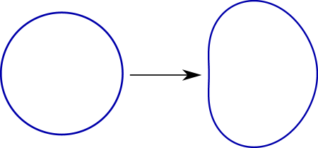
Figure 1: Approximate traveling wave shape with velocity $V=0.22$ bifurcated from a radial steady state with $R=4$, $\beta=5/8$. The shape captures terms up to third order in $V$ computed as detailed in Appendix A.

Fig. 1 illustrates the change in shape when the radially symmetric steady state bifurcates to a non-radial traveling wave. The calculations are presented in the Appendix A.

7 Nonradial steady states

While the main focus of this work is on traveling wave solutions, we also establish existence of steady state solutions lacking radial symmetry which, like traveling waves, form branches bifurcating from the family of radially symmetric steady states. Our analysis is restricted to bifurcation from pointwise minimal solutions of (2.1)-(2.2), whose existence is guaranteed by statement (ii) of Theorem (2.2).

As before we fix $R>0$ and perform a local analysis in a neighborhood of a radially symmetric steady state $(\Lambda_{0},\Phi_{0})$. We assume that $(\Lambda_{0},\Phi_{0})\in\mathcal{A}_{1}$, and moreover that $\Phi_{0}$ is a pointwise minimal solution of (2.1)-(2.2) for $\Lambda=\Lambda_{0}$. Therefore, by Proposition (5.1) there exists a family of solutions $\Lambda=\Lambda(V,\eta,z)$ $S=S(x,y,V,\eta,z)$ of the problems (1.9)-(1.10) in domains $\Omega_{\eta}$. The problem of finding solutions of (1.9)-(1.11) with $V=0$ can be rewritten as the fixed point problem (6.10). Furthermore, in terms of the linearized operator $L_{\rho}(\,\cdot\,;z)$, given by (6.11), the necessary condition for bifurcation of steady states at $(\Lambda_{0},\Phi_{0})$ is that $1$ is an eigenvalue of $L_{\rho}(\,\cdot\,;z)$ with $V=0$ and an eigenfunction $\rho$ satisfying the orthogonality condition $\int_{-\pi}^{\pi}\rho(\varphi)\cos\varphi\,d\varphi=0$. In view of Lemma 6.2, this necessary condition can be reformulated as $E_{l}(0)=1$ for some $l=2,3,\dots$, where $E_{l}(z)$ are the eigenvalues given by (6.14).

Lemma 7.1.

Let $\Phi_{0}$ be a pointwise minimal solution of (2.1)-(2.2) with $\Lambda=\Lambda_{0}\geq 0$, and let $L_{\rho}(\,\cdot\,;z)$ be the family of linearized operators given by (6.11), such that $z=0$ corresponds to the linearization around $(\Lambda_{0},\Phi_{0})$. Then eigenvalues $E_{l}(z)$, $l=2,3,\dots$ of $L_{\rho}(\,\cdot\,;z)$, given by (6.14), are strictly increasing in $z$ for sufficiently small $z$, and if $E_{l_{1}}=E_{l_{2}}(0)=1$ for $l_{1},l_{2}\geq 2$, then $l_{1}=l_{2}$.

Proof.

Rewrite problem (6.16), which determines $h_{l}(r;z)$, in terms of the new unknown $\psi_{l}(r;z):=h_{l}(r;z)+\Phi^{\prime}(r;z)$:

$$-\frac{1}{r}(r\psi^{\prime}_{l}(r))^{\prime}+\left(\frac{l^{2}}{r^{2}}+1-\Lambda(z)e^{\Phi(r;z)}\right)\psi_{l}(r)=\frac{l^{2}-1}{r^{2}}\Phi^{\prime}(r;z)\quad 0<r<R,\quad\psi_{l}(0)=\psi_{l}(R)=0.$$ (7.1)

Since $\Phi(r;z)$ are minimal solutions of (2.1)-(2.2) for small $z$, we can employ a comparison argument to prove that $\psi_{l}(r;z_{1})<\psi_{l}(r;z_{2})$, $0<r<R$, whenever $z_{1}>z_{2}$. Indeed, we have

$$-\frac{1}{r}\bigl{(}r(\psi^{\prime}_{l}(r;z_{2})-\psi^{\prime}_{l}(r;z_{1}))\bigr{)}^{\prime}+\left(\frac{l^{2}}{r^{2}}+1-\Lambda(z_{2})e^{\Phi(r;z_{2})}\right)(\psi_{l}(r;z_{2})-\psi_{l}(r;z_{1}))$$ (7.2)

$$=~{}\frac{l^{2}-1}{r^{2}}(\Phi^{\prime}(r;z_{2})-\Phi^{\prime}(r;z_{1}))+(\Lambda(z_{2})e^{\Phi(r;z_{2})}-\Lambda(z_{1})e^{\Phi(r;z_{1})})\psi_{l}(r;z_{1}).$$

Using factorization idea as in Lemma 4.1 we can show that every solution of (7.1) is negative in $(0,R)$, therefore the last term in (7.2) is positive. The same factorization trick applied to the equation

$$-\frac{1}{r}\bigl{(}r(\Phi^{\prime}(r;z_{2})-\Phi^{\prime}(r;z_{1}))^{\prime}\bigr{)}^{\prime}+ \left(\frac{1}{r^{2}}+1-\Lambda(z_{2})e^{\Phi(r;z_{2})}\right)(\Phi^{\prime}(r;z_{2})-\Phi^{\prime}(r;z_{1}))$$

$$= (\Lambda(z_{2})e^{\Phi(r;z_{2})}-\Lambda(z_{1})e^{\Phi(r;z_{1})})\Phi^{\prime}(r;z_{1})$$

shows that $\Phi^{\prime}(r;z_{2})-\Phi^{\prime}(r;z_{1})>0$ if $\Phi(r;z_{1})>\Phi(r;z_{2})$ on $(0,R)$ and $\Lambda(z_{1})>\Lambda(z_{2})$. Thus the right hand side of (7.2) is positive and the inequality $\psi_{l}(r;z_{1})<\psi_{l}(r;z_{2})$ follows. Moreover the Hopf Lemma applied after a proper factorization (again as in Lemma 4.1) implies that $\psi_{l}^{\prime}(R;z_{1})<\psi_{l}^{\prime}(R;z_{2})$. This proves monotonicity of $E_{l}(z)$.

To complete the proof of the Lemma assume by contradiction that $E_{l_{1}}(0)=E_{l_{2}}(0)$ for different $l_{1},l_{2}\geq 2$, say $l_{1}>l_{2}$. Then by (6.14) we have

$$\psi_{l_{1}}^{\prime}(R;0)/(l_{1}^{2}-1)=\psi_{l_{2}}^{\prime}(R;0)/(l_{2}^{2}-1)=\beta/R^{2}.$$ (7.3)

On the other hand functions $\psi_{l_{i}}^{\prime}(r;0)/(l_{i}^{2}-1)$, $i=1,2$ solve

$$-\frac{1}{r}(r\psi^{\prime}_{l_{i}}/(l_{i}^{2}-1))^{\prime}+\left(\frac{l^{2}_{i}}{r^{2}}+1-\Lambda_{0}e^{\Phi_{0}}\right)\psi_{l_{i}}/(l_{i}^{2}-1)=\frac{1}{r^{2}}\Phi^{\prime}_{0},\quad 0<r<R.$$ (7.4)

Then the pointwise inequalities $0>\psi_{l_{1}}>\psi_{l_{2}}$ on $(0,R)$ follow, and we have $\psi_{l_{1}}^{\prime}(R;0)/(l_{1}^{2}-1)<\psi_{l_{2}}^{\prime}(R;0)/(l_{2}^{2}-1)$, contradiction. ∎

The following theorem establishes the existence of bifurcations to not radially symmetric steady states if the surface tension parameter $\beta$ is sufficiently small.

Theorem 7.2.

Given $R>0$, and $l=2,3,\dots$, for sufficiently small $\beta>0$ there is a family of steady states solutions of (1.6)-(1.8) whith the domian $\Omega$ whose boundary is given by

$$\partial\Omega=\{(x,y)=(R+\rho_{\delta}(\varphi))(\cos\varphi,\sin\varphi)\,|\,-\pi\leq\varphi<\pi\},\quad\text{where}\ \rho_{\delta}=\delta\cos l\varphi+o(\delta),$$ (7.5)

and $\delta>0$ is a small parameter.

Proof.

The argument follows the line of Theorem 6.4. The bifurcation condition (3.8) for traveling waves is now replaced by

$$\frac{\psi_{l}^{\prime}(R;0)}{l^{2}-1}=\beta/R^{2},$$ (7.6)

where $\psi_{l}(r;0)$ is a solution of (7.1) for $z=0$, and this latter condition is always satisfied at some pair $(\Lambda_{0},\Phi_{0})\in\mathcal{A}_{0}$ , provided $\beta>0$ is sufficiently small. Note that in contrast to (3.8) the condition (7.6) depends on $\beta$. Considering $\beta>0$ so small that the eigenvalues $E_{0,1}(z)$ (of the linearized operator $\overline{L}(\,\cdot\,;z)$), given by (6.13), are bounded away from $1$, and using Lemma 7.1 we see that for sufficiently small $z$ only the eigenvalue $E_{l}(z)$ takes value $1$ and the sign of $E_{l}(z)-1$ changes. This allows us to establish the bifurcation of non-radial steady states analogously to Theorem 6.4.∎

8 Conclusions

We consider a two dimensional Keller-Segel type elliptic-parabolic system with free boundary governed by a nonlocal kinematic condition which involves boundary curvature. This system models the motility of a eukaryotic cell on a flat substrate and is obtained as a reduction [32] of the more complicated model from [3]. We show that the model captures the main biological features of cell motility such as persistent motion and breaking of symmetry which have been studied in numerous experimental works, e.g., [3, 24]. In the model under consideration these two features correspond to bifurcation from radial steady states to non-radial steady states and traveling waves. In particular, our analytical and numerical calculations capture emergence of asymmetric shapes of the traveling waves in this bifurcation, see Fig. 1. Specifically, the asymmetry of the cell shape depicted on Fig. 1 qualitatively agrees with that of an actual moving cell as observed in [4].

The results are obtained by a two step procedure. First we reduce the problem of finding traveling waves/steady states to a Liouville type equation with an additional boundary condition due to the free boundary setting. Using methods from [10] based on the Implicit Function Theorem, we further reduce the problem to a fixed point problem for a nonlinear compact mapping. Second, Leray-Schauder degree theory is applied to the this fixed point problem to prove existence of both traveling waves and nonradial steady states.

Acknowledgments. Work of LB, JF, VR was partially supported by NSF grant DMS-1405769. The work of VR was also partially supported by the PSU Center “Mathematics of Living and Mimetic Matter”. The authors are thankful to PSU students Matthew Mizuhara and Hai Chi for careful reading of the manuscript and suggestions leading to its improvement. We also would like to acknowledge numerous fruitful discussions with our colleagues A. Mogilner and L. Truskinovsky.

Appendix A Asymptotic expansion of traveling waves near bifurcation point and emergence of asymmetric shapes

In this Appendix we construct several terms of the asymptotic expansion of the free boundary problem (1.9)-(1.11). This is done for the case when the necessary bifurcation condition (3.8)(Section 3) is satisfied on a pair $(\Lambda_{0},\Phi_{0})$ with $\Phi_{0}$ being a minimal solution of (2.1)-(2.2). Then the bifurcating traveling waves can be expanded in a (formal) series in a small parameter $\varepsilon:=V$. This expansion can be rigorously justified using Lyapunov-Schmidt reduction. While the first order approximation is already introduced in Section 3, here we calculate the first three terms in this asymptotic expansion and justify the assumption that the first order correction to $\Lambda_{0}$ is zero. Note that the first order correction to the shape of the domain is zero, the second order is symmetric with respect to the $y$-axis, and the asymmetry emerges in the third correction term.

We seek the unknown domain $\Omega$ in the form $\Omega=\{(r\cos\varphi,r\sin\varphi)\mid\varphi\in[-\pi,\pi),0\leq r<R+\rho(\varphi)\}$ and introduce the following expansions for the solutions of (1.9)-(1.11)

$$\rho=\varepsilon\rho_{1}+\varepsilon^{2}\rho_{2}+\varepsilon^{3}\rho_{3}+O(\varepsilon^{4}),\quad S=\Phi_{0}(r)+\varepsilon S_{1}+\varepsilon^{2}S_{2}+\varepsilon^{3}S_{3}+O(\varepsilon^{4}),$$

$$\Lambda=\Lambda_{0}+\varepsilon\Lambda_{1}+\varepsilon^{2}\Lambda_{2}+\varepsilon^{3}\Lambda_{3}+O(\varepsilon^{4}),\quad\text{and}\quad\lambda=\lambda_{0}+\varepsilon\lambda_{1}+\varepsilon^{2}\lambda_{2}+\varepsilon^{3}\lambda_{3}+O(\varepsilon^{4}),$$

where $\lambda_{0}={\beta}/{R}-\Phi^{\prime}_{0}(R)$ follows from the leading term in the expansion of (1.11) in $\varepsilon=V$. Plugging the above expansions into (1.9)-(1.11) and equating the terms of order $\varepsilon$, $\varepsilon^{2}$, $\varepsilon^{3}$ yields the following equations

$$-\Delta S_{1}+S_{1}=\Lambda_{0}e^{\Phi_{0}(r)}(S_{1}-x)+\Lambda_{1}e^{\Phi_{0}(r)},$$ (A.1)

$$-\Delta S_{2}+S_{2}=\Lambda_{0}e^{\Phi_{0}(r)}S_{2}+\frac{\Lambda_{0}}{2}e^{\Phi_{0}(r)}(S_{1}-x)^{2}+\Lambda_{1}e^{\Phi_{0}(r)}(S_{1}-x)+\Lambda_{2}e^{\Phi_{0}(r)},$$ (A.2)

$$-\Delta S_{3}+S_{3}-\Lambda_{0}e^{\Phi_{0}(r)}S_{3}= \Lambda_{0}e^{\Phi_{0}(r)}\left((S_{1}-x)S_{2}+(S_{1}-x)^{3}/6\right)$$ (A.3)

$$+\Lambda_{1}e^{\Phi_{0}(r)}\left(S_{2}+(S_{1}-x)^{2}/2\right)+\Lambda_{2}e^{\Phi_{0}(r)}(S_{1}-x)+\Lambda_{3}e^{\Phi_{0}(r)}$$

in $B_{R}$ with boundary conditions

$$S_{1}(R,\varphi)+\Phi_{0}^{\prime}(R)\rho_{1}(\varphi)=0$$ (A.4)

$$S_{2}(R,\varphi)+\Phi_{0}^{\prime}(R)\rho_{2}(\varphi)=T_{1}(\varphi)$$ (A.5)

$$S_{3}(R,\varphi)+\Phi_{0}^{\prime}(R)\rho_{3}(\varphi)=-\partial_{r}S_{1}(R,\varphi)\rho_{2}+T_{2}(\varphi)$$ (A.6)

and

$$\cos\varphi=\partial_{r}S_{1}(R,\varphi)+\Phi_{0}^{\prime\prime}(R)\rho_{1}(\varphi)+\frac{\beta}{R^{2}}(\rho_{1}^{\prime\prime}(\varphi)+\rho_{1}(\varphi))+\lambda_{1},$$ (A.7)

$$0=\partial_{r}S_{2}(R,\varphi)+\Phi_{0}^{\prime\prime}(R)\rho_{2}(\varphi)+\frac{\beta}{R^{2}}(\rho^{\prime\prime}_{2}(\varphi)+\rho_{2}(\varphi))+T_{3}(\varphi)+\lambda_{2}$$ (A.8)

$$\frac{1}{R}\rho_{2}^{\prime}(\varphi)\sin\varphi= \partial_{r}S_{3}(R,\varphi)+\Phi_{0}^{\prime\prime}(R)\rho_{3}(\varphi)$$ (A.9)

$$+\partial^{2}_{r}S_{1}(R,\varphi)\rho_{2}(\varphi)-\partial_{\varphi}S_{1}(R,\varphi)\frac{\rho_{2}^{\prime}(\varphi)}{R^{2}}+\frac{\beta}{R^{2}}(\rho^{\prime\prime}_{3}(\varphi)+\rho_{3}(\varphi))+T_{4}(\varphi)+\lambda_{3},$$

where $T_{i}$, $i=1,\dots 4$ denote various terms containing factors $\rho_{1}(\varphi)$ or $\rho^{\prime}_{1}(\varphi)$ which will be shown to vanish.

As explained in Section (6), due to the symmetry of the problem we only consider even functions $\rho$. Moreover we impose the condition that the area of $\Omega$ is equal to that of the disc $B_{R}$ and fix the center of mass of the domain at the origin to get rid of solutions obtained by infinitesimal shifts of the domain. To the order $\varepsilon$ these two conditions yield

$$\int_{-\pi}^{\pi}\rho_{1}\,d\varphi=0,\quad\int_{-\pi}^{\pi}\rho_{1}\cos\varphi\,d\varphi=0.$$ (A.10)

Since $\Phi_{0}$ is a minimal solution of (2.1)-(2.2) we can locally parametrize solutions $(\Lambda,\Phi(r,\Lambda))$ of (2.1)-(2.2) by $\Lambda$ so that $\Phi_{0}(r)=\Phi(r,\Lambda_{0})$. Expanding $\rho_{1}$ into a Fourier series $\rho_{1}=\sum c_{l}\cos l\varphi$ we find from (A.1),(A.4) that

$$S_{1}=\tilde{\phi}(r,\Lambda_{0})\cos\varphi+\Lambda_{1}\partial_{\Lambda}\Phi(r,\Lambda_{0})+\sum c_{l}h_{l}(r)\cos l\varphi,$$

where $\tilde{\phi}(r,\Lambda)$ are solutions of (3.6)-(3.7) and $h_{l}$ are solutions of problems (6.16) with $\Lambda=\Lambda_{0}$ and $\Phi=\Phi_{0}$ (since $\Phi_{0}$ is a minimal solution of (2.1)-(2.2), solutions $h_{l}$ of (6.16) are defined uniquely). By (A.10) the first Fourier coefficients satisfy $c_{0}=c_{1}=0$. Moreover, assuming that the condition (6.17) is satisfied we find by virtue of (A.7) that all other Fourier coefficients $c_{l}$ are also zero, i.e. $\rho_{1}=0$. Thus

$$S_{1}=\tilde{\phi}(r,\Lambda_{0})\cos\varphi+\Lambda_{1}\partial_{\Lambda}\Phi(r,\Lambda_{0})$$ (A.11)

(next we show that actually $\Lambda_{1}=0$).

Similarly to above considerations, applying Fourier analysis to problem (A.2),(A.5), (A.8) we find

$$S_{2}=\Lambda_{1}\partial_{\Lambda}\tilde{\phi}(r,\Lambda_{0})\cos\varphi+\tilde{S}_{2}(r)\cos 2\varphi+G(r),\quad\rho_{2}=-\frac{\tilde{S}_{2}(R)}{\Phi_{0}^{\prime}(R)}\cos 2\varphi,$$ (A.12)

where $\tilde{S}_{2}$ solves

$$-\tilde{S}_{2}^{\prime\prime}-\frac{1}{r}\tilde{S}_{2}^{\prime}+(1+4/r^{2})\tilde{S}_{2}-\Lambda_{0}e^{\Phi_{0}(r)}\tilde{S}_{2}=\frac{\Lambda_{0}}{4}e^{\Phi_{0}(r)}(\tilde{\phi}(r,\Lambda_{0})-r)^{2}$$ (A.13)

on $(0,R)$ with

$$\tilde{S}_{2}(0)=0,\quad\tilde{S}_{2}^{\prime}(R)=\frac{\Phi_{0}^{\prime\prime}(R)-3\beta/R^{2}}{\Phi_{0}^{\prime}(R)}\tilde{S}_{2}(R),$$ (A.14)

and $G(r)$ is some function whose particular form is not important for the further analysis. Note that under the condition (6.17) problem (A.13)-(A.14) has a unique solution.

Considering the Fourier mode corresponding to $\cos\varphi$ in (A.8) we obtain that $\Lambda_{1}=0$, provided that $\partial_{\Lambda}\tilde{\phi}^{\prime}(R,\Lambda_{0})\not=0$. The latter inequality is proved as follows. Multiply (3.6) by $\Phi^{\prime}(r,\Lambda)r$ and integrate from $0$ to $R$ to find that

$$\tilde{\phi}^{\prime}(R,\Lambda)=\frac{\Lambda}{R\Phi^{\prime}(R,\Lambda)}\int_{0}^{R}e^{\Phi(r,\Lambda)}\Phi^{\prime}(r,\Lambda)r^{2}\,dr=1+\frac{\Lambda R^{2}-\int_{0}^{R}\Phi(r,\Lambda)r\,dr-\Lambda\int_{0}^{R}e^{\Phi(r,\Lambda)}r\,dr}{\int_{0}^{R}\Phi(r,\Lambda)r\,dr-\Lambda\int_{0}^{R}e^{\Phi(r,\Lambda)}r\,dr}.$$ (A.15)

Then

$$\partial_{\Lambda}\tilde{\phi}^{\prime}(R,\Lambda_{0})>\frac{R^{2}-\int_{0}^{R}\partial_{\Lambda}\Phi(r,\Lambda_{0})r\,dr-\int_{0}^{R}e^{\Phi(r,\Lambda_{0})}r\,dr}{\int_{0}^{R}\Phi(r,\Lambda_{0})r\,dr-\Lambda_{0}\int_{0}^{R}e^{\Phi(r,\Lambda_{0})}r\,dr},$$ (A.16)

where we have used the fact that minimal solutions $\Phi(r,\Lambda)$ are increasing in $\Lambda$ and the denominator in (A.15) is negative. Since the pair $(\Lambda,\Phi)=(\Lambda_{0},\Phi_{0})$ satisfies (3.9) we have

$$\partial_{\Lambda}\tilde{\phi}^{\prime}(R,\Lambda_{0})>-\frac{\int_{0}^{R}(\partial_{\Lambda}\Phi(r,\Lambda_{0})-\Phi(r,\Lambda_{0})/\Lambda_{0})r\,dr}{\int_{0}^{R}\Phi(r,\Lambda_{0})r\,dr-\Lambda_{0}\int_{0}^{R}e^{\Phi(r,\Lambda_{0})}r\,dr}.$$ (A.17)

Furthermore we obtain that the function $w=\partial_{\Lambda}\Phi(r,\Lambda_{0})-\Phi(r,\Lambda_{0})/\Lambda_{0}$ is positive applying the maximum principle to the equation $-\Delta w+w=\Lambda_{0}e^{\Phi_{0}(r)}\partial_{\Lambda}\Phi(r,\Lambda_{0})>0$. Thus $\partial_{\Lambda}\tilde{\phi}^{\prime}(R,\Lambda_{0})>0$.

Finally, to identify $S_{3}$ and $\rho_{3}$ we apply Fourier analysis to (A.3),(A.6), (A.9). The resulting formula for $\rho_{3}$ is

$$\rho_{3}=-\frac{\tilde{S}_{3}(R)}{\Phi_{0}^{\prime}(R)}\cos 3\varphi,$$ (A.18)

where $\tilde{S}_{3}$ is the solution of the equation

$$-\tilde{S}_{3}^{\prime\prime}-\frac{1}{r}\tilde{S}_{3}^{\prime}+(1+9/r^{2})\tilde{S}_{3}-\Lambda_{0}e^{\Phi_{0}(r)}\tilde{S}_{3}=\frac{\Lambda_{0}}{2}e^{\Phi_{0}(r)}(\tilde{\phi}(r)-r)\tilde{S}_{2}(r)+\frac{\Lambda_{0}}{24}e^{\Phi_{0}(r)}(\tilde{\phi}(r)-r)^{3}$$ (A.19)

on $(0,R)$ with boundary conditions

$$\tilde{S}_{3}(0)=0,\quad\tilde{S}_{3}^{\prime}(R)=\frac{\Phi_{0}^{\prime\prime}(R)-8\beta/R^{2}}{\Phi_{0}^{\prime}(R)}\tilde{S}_{3}(R)+\frac{\tilde{\phi}^{\prime\prime}(R)-2/R}{2\Phi_{0}^{\prime}(R)}\tilde{S}_{2}(R).$$ (A.20)

Thus the first terms of the asymptotic expansion of the function $\rho$ which determine the shape of the domain are

$$\rho=-\varepsilon^{2}\frac{\tilde{S}_{2}(R)}{\Phi_{0}^{\prime}(R)}\cos 2\varphi-\varepsilon^{3}\frac{\tilde{S}_{3}(R)}{\Phi_{0}^{\prime}(R)}\cos 3\varphi+\dots$$ (A.21)

where $\tilde{S}_{2}$ solves (A.13)-(A.14), $\tilde{S}_{3}$ solves (A.19)-(A.20) and $\tilde{\phi}$ is a solution of (3.6)-(3.7) with $\Lambda=\Lambda_{0}$ and $\Phi=\Phi_{0}$.

References

- [1] J. Allard and A. Mogilner. Traveling waves in actin dynamics and cell motility. Curr Opin Cell Biol, 25:107–115, 2013.
- [2] W. Alt and M. Dembo. Cytoplasm dynamics and cell motion: two-phase flow models. Math Biosci, 156:207–228.
- [3] E. Barnhart, K. Lee, G. M. Allen, J. A. Theriot, and A. Mogilner. Balance between cell-substrate adhesion and myosin contraction determines the frequency of motility initiation in fish keratocytes. Proc Natl Acad Sci U.S.A., 112(16):5045–5050, 2015.
- [4] E. Barnhart, K. Lee, K. Keren, A. Mogilner, and J. A. Theriot. An adhesion-dependent switch between mechanisms that determine motile cell shape. PLoS Biology, 9(5):e1001059, 2011.
- [5] L. Berlyand, M. Potomkin, and V. Rybalko. Phase-field model of cell motility: Traveling waves and sharp interface limit. Comptes Rendus Mathematique, 354(10):986–992, 2016.
- [6] H. Brezis and F. Merle. Uniform estimates and blow-up behavior for solutions of in two dimensions. Comm PDE, 16:1223–1253, 1991.
- [7] H. Byrne and D. Drasdo. Individual-based and continuum models of growing cell populations: a comparison. J Math Biol, 58:657–687, 2009.
- [8] E. Caglioti, P.-L. Lions, C. Marchioro, and M. Pulvirenti. A special class of stationary flows for two-dimensional euler equations: a statistical mechanics description. Comm Math Phys, 143(3):501–525, 1992.
- [9] F. Cerreti, B. Perthame, C. Schmeiser, M. Tang, and N. Vauchelet. Waves for a hyperbolic keller-segel model and branching instabilities. Mathematical Models and Methods in Applied Sciences, 21(supp01):825–842, 2011.
- [10] M. G. Crandall and P. H. Rabinowitz. Bifurcation from simple eigenvalues. J Funct Anal, 8:321–340, 1971.
- [11] A. Friedman. Free boundary problems in science and technology. Notices of the AMS, 47(8):854–861, 2000.
- [12] A. Friedman. Pde problems arising in mathematical biology. Networks & Heterogeneous Media, 7(4), 2012.
- [13] A. Friedman and F. Reitich. Symmetry-breaking bifurcation of analytic solutions to free boundary problems: an application to a model of tumor growth. Transactions of the American Mathematical Society, 353(4):1587–1634, 2001.
- [14] B. Gidas, W.-M. Ni, and L. Nirenberg. Symmetry and related properties via the maximum principle. Comm Math Phys, 68:209–243, 1979.
- [15] D. Gilbarg and N. S. Trudinger. Elliptic Partial Differential Equations of Second Order. Classics in Mathematics. Springer, Berlin Heidelberg New York, reprint of 2nd edition, 2001.
- [16] W. Hao, J. D. Hauenstein, B. Hu, Y. Liu, A. J. Sommese, and Y. T. Zhang. Bifurcation for a free boundary problem modeling the growth of a tumor with a necrotic core. Nonlinear Analysis: Real World Applications, 13(2):694–709, 2012.
- [17] T. Hillen and K. Painter. A user’s guide to pde models for chemotaxis. J Math Biol, 58(3,4):183–217, 2009.
- [18] Yaodan Huang, Zhengce Zhang, and Bei Hu. Bifurcation for a free-boundary tumor model with angiogenesis. Nonlinear Analysis: Real World Applications, 35:483–502, 2017.
- [19] E. Javierre, F. J. Vermolen, C. Vuik, and S. van der Zwaag. A mathematical analysis of physiological and morphological aspects of wound closure. J Math Biol, 59(10):605–630, 2009.
- [20] J. Keener and H. Keller. Positive solutions of convex nonlinear eigenvalue problems. J Diff Eqn, 16(1):103–125, 1974.
- [21] E. Keller and L. Segel. Initiation of slime mold aggregation viewed as an instability. J Theor Biol, 26:399–415, 1970.
- [22] E. Keller and L. Segel. Model for chemotaxis. J Theor Biol, 30:225–234, 1971.
- [23] E. Keller and L. Segel. Traveling bands of chemotactic bacteria: a theoretical analysis. J Theor Biol, 30:235–248, 1971.
- [24] K. Keren, Z. Pincus, G. Allen, E. Barnhart, G. Marriott, A. Mogilner, and J. Theriot. Mechanism of shape determination in motile cells. Nature, 453(7194):475–480, 2008.
- [25] P. Korman. Global Solution Curves for Semilinear Elliptic Equations. World Scientific Publishing, Singapore, 2012.
- [26] M. A. Krasnosel’skii, E. M. Lifshits, and A. V. Sobolev. Positive linear systems: the method of positive operators. Heldermann Verlag, 1989.
- [27] Y. Y. Li. Harnack type inequality: the method of moving planes. Comm Math Phys, 200(2):421–444, 1999.
- [28] C.-S. Lin. An expository survey on the recent development of mean field equations. Discrete Contin Dyn Syst, 19(2):387–410, 2007.
- [29] J. Liouville. Sur l’equation aux difference partielles . C R Acad Sci Paris, 36:71–72, 1853.
- [30] J. S. Lowengrub, H. B. Frieboes, F. Jin, Y. L. Chuang, X. Li, P. Macklin, S. M. Wise, and V. Cristini. Nonlinear modelling of cancer: bridging the gap between cells and tumours. Nonlinearity, 23(1):R1, 2009.
- [31] J. Mawhin. Leray-schauder degree: a half century of extensions and applications. Topol Methods Nonlinear Anal, 14(2):195–228, 1999.
- [32] A. Mogilner. Private communication.
- [33] M. Nolasco and G. Tarantello. On a sharp sobolev-type inequality on two-dimensional compact manifolds. Arch Rational Mech Anal, 145(2):161–195, 1998.
- [34] B. Perthame, M. Tang, and N. Vauchelet. Traveling wave solution of the hele-shaw model of tumor growth with nutrient. Math Models Methods Appl Sci, 24(13):2601–2626, 2014.
- [35] B. Perthame and A. Vasseur. Regularization in keller-segel type systems and the de giorgi method. Commun Math Sci, 10(2):463–476, 2012.
- [36] P. Recho, T. Putelat, and L. Truskinovsky. Contraction-driven cell motility. Phys Rev Lett, 111(10):108102, 2013.
- [37] P. Recho, T. Putelat, and L. Truskinovsky. Mechanics of motility initiation and motility arrest in crawling cells. Journal of Mechanics Physics of Solids, 84:469–505, 2015.
- [38] P. Recho and L. Truskinovsky. Cell locomotion in one dimension. In Physical Models of Cell Motility, Springer, I.S. Aranson(ed), pages 135–197, 2016.
- [39] D. Shao, H. Levine, and J. W. Rappel. Coupling actin flow, adhesion, and morphology in a computational cell motility model. Proc Nat Acad Sci, 109(18):6851–6856, 2012.
- [40] D. Shao, W. J. Rappel, and H. Levine. Computational model for cell morphodynamics. Phys. Rev. Lett., 105:108104, 2010.
- [41] T. Suzuki. Global analysis for a two-dimensional elliptic eigenvalue problem with the exponential nonlinearity. Annales de l’I.H.P. Analyse non linéaire, 9(4):367–397, 1992.
- [42] B. Vanderlei, J. J. Feng, and L. Edelstein-Keshet. A computational model of cell polarization and motility coupling mechanics and biochemistry. Multiscale Model Simul, 9(4):1420–1443, 2011.
- [43] M. Winkler. The two-dimensional keller-segel system with singular sensitivity and signal absorption: global large data solutions and their relaxation properties. Mathematical Models and Methods in Applied Sciences, 26:987–1024, 2016.
- [44] M. Winkler and K. C. Djie. Boundedness and finite-time collapse in a chemotaxis system with volume-filling effect. Nonlinear Analysis: Theory, Methods and Applications, 72(2):1044 – 1064, 2010.
- [45] G. Wolansky. A critical parabolic estimate and application to nonlocal equations arising in chemotaxis. Applicable Analysis, 66:291–321, 1997.
- [46] F. Ziebert and I S Aranson. Computational approaches to substrate-based cell motility. Npj Computational Materials, 2:16019, 2016.
- [47] F. Ziebert, S. Swaminathan, and I. S. Aranson. Model for self-polarization and motility of keratocyte fragments. J. R. Soc. Interface, 9:1084–1092, 2012.