A Generalized Model of Social and Biological Contagion

Abstract

We present a model of contagion that unifies and generalizes existing models of the spread of social influences and microorganismal infections. Our model incorporates individual memory of exposure to a contagious entity (e.g., a rumor or disease), variable magnitudes of exposure (dose sizes), and heterogeneity in the susceptibility of individuals. Through analysis and simulation, we examine in detail the case where individuals may recover from an infection and then immediately become susceptible again (analogous to the so-called SIS model). We identify three basic classes of contagion models which we call epidemic threshold, vanishing critical mass, and critical mass classes, where each class of models corresponds to different strategies for prevention or facilitation. We find that the conditions for a particular contagion model to belong to one of the these three classes depend only on memory length and the probabilities of being infected by one and two exposures respectively. These parameters are in principle measurable for real contagious influences or entities, thus yielding empirical implications for our model. We also study the case where individuals attain permanent immunity once recovered, finding that epidemics inevitably die out but may be surprisingly persistent when individuals possess memory.

Journal of Theoretical Biology, 232, 587–604, 2005.

I Introduction

Contagion, in its most general sense, is the spreading of an entity or influence between individuals in a population, via direct or indirect contact. Contagion processes therefore arise broadly in the social and biological sciences, manifested as, for example, the spread of infectious diseases (murray2002, ; daley1999, ; anderson1991a, ; brauer2001, ; diekmann2000, ; hethcote2000, ) and computer viruses, the diffusion of innovations (coleman1966, ; valente1995, ; rogers2003, ), political upheavals (lohmann1994, ), and the dissemination of religious doctrine (stark1996, ; montgomery1996, ). Existing mathematical models of contagion, while motivated in a variety of ways depending on the application at hand, fall into one of only two broad categories, where the critical distinction between these categories can be explained in terms of the interdependencies between successive contacts; that is, the extent to which the effect of an exposure to a contagious agent is determined by the presence or absence of previous exposures.

The standard assumption in all mathematical models of infectious disease spreading (for example, the classic SIR model (kermack1927, ; murray2002, )), and also in some models of social contagion (goffman1964, ; daley1965, ; bass1969, ), is that there is no interdependency between contacts; rather, the infection probability is assumed to be independent and identical across successive contacts. All such models therefore fall into a category that we call independent interaction models. By contrast, what we call threshold models assert that an individual can only become infected when a certain critical number of exposures has been exceeded, at which point infection becomes highly probable. The presence of a threshold corresponds to interdependencies of an especially strong nature: contacts that occur when an individual is near its threshold are extremely consequential while others have little or no effect. Threshold models are often used to describe social contagion (e.g., the spreading of fads or rumors), where individuals either deterministically (schelling1973, ; granovetter1978, ; watts2002, ) or stochastically (bikhchandani1992, ; banerjee1992, ; morris2000, ; brock2001, ) “decide” whether or not to adopt a certain behavior based in part or in whole on the previous decisions of others.

An alternative way to think about the interdependence of successive events is in terms of memory: threshold models implicitly assume the presence of memory while independent interaction models assume (again implicitly) that the infection process is memoryless . Neither class of model, however, is able to capture the dynamics of contagious processes that possess an intermediate level of interdependency, or equivalently a variable emphasis on memory. Furthermore, the relationship between interdependent interaction models, threshold models, and any possible intermediate models is unclear. Motivated by these observations, our model seeks to connect threshold and independent interaction models both conceptually and analytically, and explore the classes of contagion models that lie between them. Such an analysis is clearly relevant to problems of social contagion, in which memory of past events obviously plays some role, but one that may be less strong than is assumed by most threshold models. However, it may also be relevant to biological disease spreading models, which, to our knowledge, have previously not questioned the assumption of independence between successive exposures. While the independence assumption is indeed plausible, it has not been demonstrated empirically, and little enough is understood of the dynamics of immune system response that the alternative—persistent sub-critical doses of an infectious agent combining to generate a critical dose—cannot be ruled out. Furthermore, memory effects are known to be inherent to certain kinds of immune system responses, such as allergic response. Hence if, as we indeed show, only a slight departure from complete independence is required to alter the corresponding collective dynamics, then our approach may also shed light on the spread of infectious diseases.

II Descripton of Model

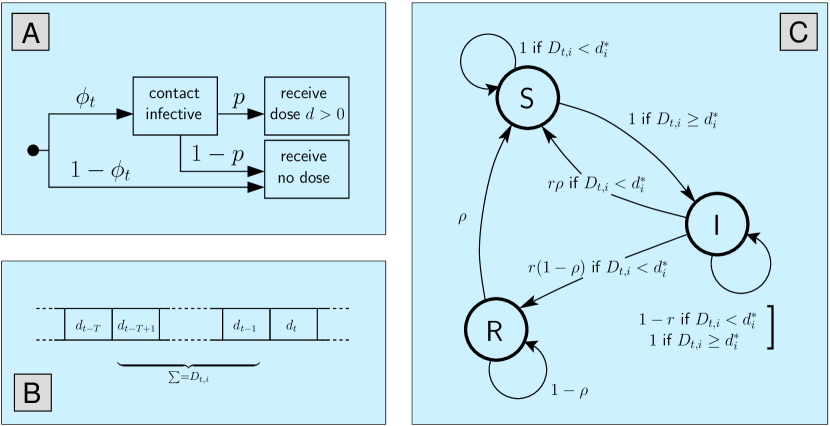
Figure 1: (A) Representation of how an individual’s dose at time $t$ is determined. At each time step, each individual, regardless of its state, contacts one other randomly chosen individual. The probability that individual $i$ contacts an infective is then $\phi_{t}$, i.e., the current fraction of infectives in the population. If the contact is infected then with probability $p$, $i$ is exposed to the contagious entity and receives a dose $d$ drawn from a fixed distribution $f$. Otherwise and also if the contacted individual is not infected in the first place (occurring with probability $1-\phi_{t}$), $i$ receives a dose of zero size. (B) Individual $i$ then updates its dose count $D_{t,i}$ by ‘forgetting’ the dose it received $T+1$ time steps ago and incorporating the current dose [Eq. (1)]. (C) Transition probabilities for individual $i$ cycling through the three states S (susceptible), I (infected), and R (recovered). If $i$ is in the susceptible state, it becomes infected with probability 1 once its dose count $D_{t,i}$ exceeds its threshold $d_{i}^{\ast}$, otherwise it remains susceptible. If $i$ becomes infected, then whenever $i$’s dose count drops below its threshold, it has a probability $r$ of recovering in each time step. Once $i$ is in state R (where it is immune to infection), it becomes susceptible again with probability $\rho$, again in each time step. Note that if $r=\rho=1$, infected individuals whose dose count falls below their threshold immediately return to the susceptible state.

Our model, aspects of which we have reported in brief elsewhere (dodds2004pa, ), comprises a population of $N$ individuals, each of which is assumed to occupy one of three states: susceptible (S); infected (I); or removed (R). Figure  1 provides a schematic representation of our model which we describe as follows. At each (discrete) time step $t$, each individual $i$ comes into contact with another individual chosen uniformly at random from the population. If the contact is infected—an event that occurs with probability $\phi_{t}$, the fraction of infectives in the population—then with probability $p$, $i$ receives a ‘dose’ $d$ drawn from a fixed dose-size distribution $f$; else $i$ receives a dose of size $0$. We call a successful transmission of a positive dose an exposure and $p$ the exposure probability. Individuals carry a memory of doses received from their last $T$ contacts and we denote the sum of individual $i$’s last $T$ doses ($i$’s dose count) at the $t$th time step by

$$D_{t,i}=\sum_{t^{\prime}=t-T+1}^{t}d_{t^{\prime},i}.$$ (1)

If $i$ is in the susceptible state, then it becomes infected once $D_{t,i}$ exceeds $i$’s dose threshold $d_{i}^{\ast}$, where $d_{i}^{\ast}$ is drawn from a given distribution $g$ (dose thresholds do not change with time). Note that we differentiate exposure from infection, the latter being the possible result of one or more exposures and only occurring once a susceptible individual’s threshold has been equaled or exceeded. Having become infected, an individual remains in state I until its dose count drops below its threshold, at which point it recovers with probability $r$ at each time step. Once recovered, an individual returns to being susceptible with probability $\rho$, again at each time step.

The probability $P_{\rm inf}$ that a susceptible individual who comes into contact with $K$ infected individuals in $T$ time steps will become infected is therefore given by

$$P_{\rm inf}(K)=\sum_{k=1}^{K}\binom{K}{k}p^{k}(1-p)^{K-k}P_{k},$$ (2)

where $K=1,\ldots,T$, and

$$P_{k}=\int_{0}^{\infty}\mbox{d}d^{\ast}g(d^{\ast})\int_{d=d^{\ast}}^{\infty}\mbox{d}d\,f^{k\star}(d)$$ (3)

Both $P_{\rm inf}(K)$ and $P_{k}$ are important quantities in our model. The quantity $P_{k}$ is the expected fraction of a population that will be infected by $k$ exposures, where the distribution $f^{k\star}(d)$, the $k$-fold convolution of $f$, is the probability that the sum of $k$ doses will be equal to $d$. The infection probability $P_{\rm inf}(K)$ gives, in effect, a dose response curve (haas2002, ) averaged over all members of the population and also the distribution of dose sizes (where we note that $K$ contacts with infected individuals will result in $k$ actual exposures with probability $\binom{K}{k}p^{k}(1-p)^{K-k}$). Figure 2 shows examples of dose response curves, calculated from Eq. (2) for four configurations of the model. The plots correspond to (A) independent interaction, (B) deterministic threshold, and, in both (C) and (D), stochastic threshold models. For the independent interaction example, a single exposure is needed to generate an infection and so exposures effectively act independently. The deterministic threshold example incorporates uniform dose sizes and thresholds, and when the probability of an exposure is set to $p=1$, the response becomes deterministic (individuals are always infected when their dose count is met or exceeded and never otherwise); but now the threshold can only be exceeded by multiple infections. The two stochastic cases generalize the deterministic case by allowing (C) dose sizes to be heterogeneous, and (D) both dose sizes and thresholds to be heterogeneous.

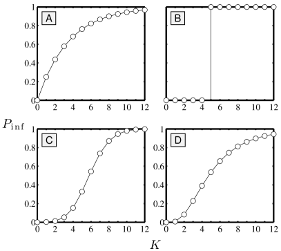
Figure 2: Examples of dose response, i.e., $P_{\rm inf}(K)$, the probability an individual becomes infected due to $K$ exposures in the last $T(=12)$ time steps [see Eq. (2)]. The plots correspond to (A) independent interaction (or disease-like) models with homogeneous dose sizes and thresholds [$p=0.25$, dose distribution $f(d)=\delta(d-1)$, and threshold distribution $g(d^{\ast})=\delta(d^{\ast}-1)$]; (B) deterministic threshold models with homogeneous dose sizes and thresholds [$p=1$, $f(d)=\delta(d-1)$, and $g(d^{\ast})=\delta(d^{\ast}-5)$]; (C) stochastic threshold models with heterogeneous doses and homogeneous thresholds [$p=0.9$, doses distributed lognormally with unit mean and standard deviation $0.5$, and $g(d^{\ast})=\delta(d^{\ast}-5)$]; and (D), same as (C) but with heterogeneity in thresholds introduced via a lognormal distribution with mean of 5 as per (C) and standard deviation of 10.

We explore the behavior of our model with respect to three qualitative types of dynamics: (1) permanent removal ($\rho=0$) dynamics, analogous to so-called SIR models in mathematical epidemiology in which individuals either die or acquire permanent immunity; (2) temporary removal ($1>\rho>0$) dynamics, analogous to SIRS models where recovered individuals become susceptible again after a certain period of immunity; and (3) instantaneous replacement ($\rho=1$) dynamics, analogous to SIS models, where infected individuals immediately become susceptible again upon recovery. Chicken pox, for example, would correspond to SIR-type contagion, while the common cold resembles the SIRS case. Because of its simplicity, we obtain the majority of our analytic results for the somewhat special SIS case ($\rho=1$). However, our main findings for the SIS case have analogs in the more complicated SIRS and SIR cases which we investigate with numerical simulations. Furthermore, while the assumption of instantaneous re-susceptibility is probably not appropriate in the case of contagious biological agents (where recovery is generally associated with some period of immunity), it may well be approximately true for contagious social influences, such as “social smoking,” where an individual, having quit, can restart immediately. A summary of the main parameters of the model and their definitions is provided in Table 1.

$T$	length of memory window
$p$	probability of exposure given contact with infective
$r$	probability of moving from infected to recovered state
$\rho$	probability of moving from immune to susceptible state
$f(d)$	distribution of dose sizes $d$
$g(d^{\ast})$	distribution of individual thresholds $d^{\ast}$
$\bar{d^{\ast}}$	uniform threshold of homogeneous population
$\phi_{t}$	fraction of population infected at time $t$
${\phi^{\ast}}$	steady-state fraction of population infected

Table 1: Summary of main model parameters and definitions.

We structure the remainder of the paper as follows. In section III, through analysis and simulations, we examine in detail the SIS $(\rho=1)$ version of the model for a homogeneous population, where by “homogeneous,” we mean that all doses are equal and of unit size [i.e., $f(d)=\delta(d-1)$], and that all individuals have the same threshold [i.e., $g(d^{\ast})=\delta(d^{\ast}-\bar{d^{\ast}})$]. For homogeneous populations, we find that only two universal classes of dynamics are possible: (1) epidemic threshold dynamics , according to which initial outbreaks either die out or else infect a finite fraction of the population, depending on whether or not the infectiousness $p$ exceeds a specific critical value $p_{c}$; and (2) critical mass dynamics according to which a finite fraction of the population can only ever be infected in equilibrium if the initial outbreak size itself constitutes a finite “critical mass.” Although homogeneity is a restrictive assumption for biological or social contagion, it provides a useful special case in that it illuminates the basic intuitions required to understand the more general, heterogeneous case. In section IV, we relax the homogeneity assumption and move to the richer and more realistic case of arbitrarily distributed dose sizes and individual thresholds. Here we find that three universal classes of contagion models are possible. In addition to the epidemic threshold and critical mass classes that carry over from the homogeneous case, we also find an intermediate class of vanishing critical mass dynamics in which the size of the required critical mass diminishes to zero for $p<1$. Furthermore, we determine where the transitions between these classes occur and also the conditions required for more complicated kinds of contagion models to arise. Subsequently, in section V, we explore the SIRS and SIR versions of the model, finding behavior that in many ways resembles that of the simpler SIS case. In the SIR case, for example, it is necessarily true that all epidemics eventually burn themselves out (because for $\rho=0$, the removed condition is an absorbing state). However, we find that the presence of memory may cause an epidemic to persist for a surprisingly long time. In section VI, we conclude our analysis, discussing briefly the implications of our findings for stimulating or retarding different contagious processes. Finally, in the appendices we provide detailed derivations of the analytical results from sections III and IV.

III Homogeneous SIS contagion models

III.1 Epidemic threshold models

We begin our analysis with a simple non-trivial case of our model, for which we assume that individuals are: identical (i.e., the population is homogeneous); have no memory of past interactions $(T=1)$; and, upon recovery from infection, immediately return to the susceptible state (i.e., $\rho=1$). In this limit our model coincides with the SIS version of the traditional Kermack-McKendrick model (kermack1927, ; murray2002, ), as individuals with no memory necessarily become infected upon exposure to a single infected individual [$g(d^{\ast})=\delta(d^{\ast}-1)$]. For a specified recovery time $(r\leq 1)$ (which again is identical across all individuals), the fraction of infected individuals at time $t$, $\phi_{t}$, evolves according to

$$\phi_{t+1}=p\phi_{t}+\phi_{t}(1-p\phi_{t})(1-r).$$ (4)

The first term on the right is the fraction of individuals newly infected between time $t$ and $t+1$, regardless of whether or not they were infected beforehand (the model allows for individuals to recover and be reinfected within one time step). The second term is the fraction of individuals who were infected in the preceding time step, were not infected between time $t$ and $t+1$, and did not recover.

Setting $\phi_{t}={\phi^{\ast}}$ in Eq. (4), we find the stable fixed points of the model as a function of $p$ are given by

$${\phi^{\ast}}=\left\{\begin{array}[]{ll}0&\mbox{for}\quad 0\leq p\leq r,\\ \frac{1-r/p}{1-r}&\mbox{for}\quad r<p\leq 1.\end{array}\right.$$ (5)

Furthermore, a single unstable set of fixed points is found along ${\phi^{\ast}}=0$ for $r<p\leq 1$. Thus, the standard memoryless SIS model exhibits an epidemic threshold (murray2002, ) at $p=p_{c}$, as displayed graphically in Figure 3: for $p\leq p_{c}=r$ no infection survives (${\phi^{\ast}}\equiv 0$) while for $p>p_{c}=r$, a stable, finite fraction of the population will become infected (${\phi^{\ast}}>0$). In the language of dynamical systems theory, the epidemic threshold is a transcritical bifurcation (strogatz1994, ) which lies at the intersection of two fixed point curves, where the stable curve changes to unstable at the intersection and vice versa (in statistical mechanics, such behavior is referred to as a second-order or continuous phase transition, where $(p_{c},0)$ is called the critical point (goldenfeld92, )). For the choice of parameters above, one branch of the transcritical bifurcation is the $p$-axis which is stable to the left of $p_{c}$ and unstable to the right (imagining the unphysical extension of ${\phi^{\ast}}$ to ${\phi^{\ast}}<0$, the other branch may be seen to extend from below the $p$-axis where it is unstable to above the $p$-axis where it is stable).

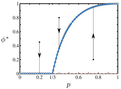
Figure 3: Fixed point curves for an example epidemic threshold model. The stable fixed point curves shown are from simulation (circles) and Eq. (10) (blue line) for $\bar{d^{\ast}}=1$, $T=2$, and $\tau=1/r-1=1$. Unstable fixed points are indicated by the dashed red line. The trajectories of three initial conditions are shown to illustrate how the level of an epidemic evolves for different values of $p$. The epidemic threshold $p_{c}=1/3$ is as predicted by $p_{c}=(T+\tau)^{-1}$, Eq. (11). For the simulation, the population size $N=10^{5}$, the number of time steps $N_{t}=10^{3}$, each data point represents the average value of ${\phi^{\ast}}(p)$ over the last $N_{s}=100$ time steps, and the initial condition is that all are infected.

We observe this kind of bifurcation structure (i.e., where the rising branch has positive slope and comprises stable equilibria) to be a robust feature with respect to a range of parameter choices, and we classify all such models as epidemic threshold models. As we show below, the same qualitative equilibrium behavior is present in all homogeneous models with dose thresholds set at $d^{\ast}=1$, even with arbitrary memory $T\geq 1$ and recovery rate $r\leq 1$. While some details of the dynamics do change as $T$ and $r$ are varied, the existence of a single transcritical bifurcation depends only on the assumption that all individuals exhibit “trivial thresholds:” $g(d^{\ast})=\delta(d^{\ast}-1)$.

First, allowing memory to be arbitrary ($T>1$) but keeping $r=1$, we observe that the individuals who are infected at some time $t$ are necessarily those who have experienced at least one infectious event in the preceding $T$ time steps; thus we obtain the following implicit equation for ${\phi^{\ast}}$,

$${\phi^{\ast}}=1-(1-p{\phi^{\ast}})^{T}.$$ (6)

As with the $T=1$ case above, the equilibrium behavior exhibits a continuous phase transition and therefore also falls into the epidemic threshold class. While we can no longer find a general, closed-form solution for ${\phi^{\ast}}$, Eq. (6) can be rearranged to give $p$ as an explicit function of ${\phi^{\ast}}$:

$$p={\phi^{\ast}}^{-1}[1-(1-{\phi^{\ast}})^{1/T}].$$ (7)

Taking the limit of ${\phi^{\ast}}\rightarrow 0$ in either Eq. (6) or Eq. (7), we find $p_{c}=1/T$. Thus, receiving at least one exposure from the last $T$ contacts is analogous to the zero memory ($T=1$), variable $r$ case above where recovery occurs on a time scale $1/r\simeq T$.

Next, we also allow the recovery rate to be arbitrary $(r<1)$. To find the fixed point curves, we modify Eq. (6) to account for the fraction of individuals that have not experienced a single exposure for at least the last $T$ time steps but have not recovered from a previous infection. We first write down the probability that an individual last experienced an infectious event $m$ time steps ago and has not yet recovered. Denoting the sequence of a positive unit dose followed by $m$ 0’s as $H_{m+1}$, we have

$$P(\mbox{infected}|H_{m+1})=p{\phi^{\ast}}(1-p{\phi^{\ast}})^{m}(1-r)^{m-T+1},$$ (8)

The first term on the right hand side of the Eq. (8) is the probability of a successful exposure; the second term is the probability of experiencing no successful exposures in the subsequent $m$ time steps; and the final term is the probability that, once the memory of the initial single exposure has been lost after $T$ time steps, the individual remains infected. Since we are only concerned with individuals who have ‘forgotten’ the source of the infection, we have $m\geq T$. Summing over $m$, we obtain the total probability that an individual was infected at least $T$ time steps ago and has not yet recovered:

$$\sum_{m=T}^{\infty}P(\mbox{infected}|H_{m+1})=\frac{p{\phi^{\ast}}(1-p{\phi^{\ast}})^{T}(1-r)}{1-(1-p{\phi^{\ast}})(1-r)}$$ (9)

Adding this fraction to the right hand side of Eq. (6) then gives

$${\phi^{\ast}} = 1-(1-p{\phi^{\ast}})^{T}\left[1-\frac{p{\phi^{\ast}}(1-r)}{1-(1-p{\phi^{\ast}})(1-r)}\right],$$ (10)

$$= 1-\frac{r(1-p{\phi^{\ast}})^{T}}{1-(1-p{\phi^{\ast}})(1-r)}.$$

Figure 3 shows a comparison between the above equation and simulation results for $T=2$, $r=1/2$, and $\bar{d^{\ast}}=1$.

Taking the limit of small ${\phi^{\ast}}$ in Eq. (10) we find the epidemic threshold to be

$$p_{c}=\frac{r}{1+r(T-1)}=\frac{1}{T+1/r-1}.$$ (11)

Checking the special cases of the preceding calculations, we find $p_{c}=r$ when $T=1$ and $p_{c}=1/T$ when $r=1$. Denoting the mean time to recovery of an infected, isolated individual by $\tau$, we observe $\tau=1/r-1$ and Eq. (11) becomes

$$p_{c}=\frac{1}{T+\tau}.$$ (12)

The time scales $T$ and $\tau$ can thus both be thought of as corresponding to two different kinds of memory, the sum of which—the total characteristic time scale of memory in the model—determines the position $p_{c}$ of the epidemic threshold. Qualitatively, therefore, all homogeneous models that possess trivial individual thresholds exhibit the same kind of equilibrium dynamics. Varying the thresholds, however, produces equilibrium behavior of a quite distinct nature, as we show in the next section.

III.2 Critical mass models

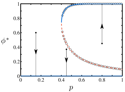
Figure 4: Comparison between simulation (circles) and theory (lines, Eq. (13)) for $T=12$, $\bar{d^{\ast}}=3$, and $r=1$. For $\bar{d^{\ast}}>1$, the homogeneous SIS contagion model exhibits a saddle-node bifurcation. Shown are the non-zero stable and unstable points. For the theoretical curves, solid lines represent stable points and dashed ones unstable points. All points on the line ${\phi^{\ast}}=0$ are stable points. The arrows show trajectories of the system for three example initial conditions. Simulations details are as per Figure 3. The location of the unstable fixed point curve is determined by binary search.

When individuals of a homogeneous population require more than one exposure to become infected—that is, when $g(d^{\ast})=\delta(d^{\ast}-\bar{d^{\ast}})$ and $\bar{d^{\ast}}>1$—the closed-form expression for the fixed points ${\phi^{\ast}}$ in the case of $r=1$ is

$${\phi^{\ast}}=\sum_{i=\bar{d^{\ast}}}^{T}\binom{T}{i}(p{\phi^{\ast}})^{i}(1-p{\phi^{\ast}})^{T-i}.$$ (13)

We now observe a fundamentally different behavior of the model: the transcritical bifurcation that is characteristic of epidemic threshold models is absent and is replaced by a saddle-node bifurcation (strogatz1994, ), an example of which is illustrated in Figure 4. We call models whose equilibrium states are determined in this manner critical mass models because, as indicated by the arrows in Figure 4, an epidemic will not spread from an infinitesimal initial outbreak, requiring instead a finite fraction of the population, or “critical mass” (schelling1978, ), to be infected initially. Saddle-node bifurcations (or backwards bifurcations) have also been observed in a number of unrelated epidemiological multi-group models, arising from differences between groups and inter-group contact rates hadeler1995 ; hadeler1997 ; dushoff1998 ; kribs-zaleta2000 ; greenhalgh2000 ; kribs-zaleta2002 .

Although it is not generally possible to obtain an expression for ${\phi^{\ast}}(p)$ from Eq. (13), we are able to write down a closed-form expression involving the position of the saddle-node bifurcation $(p_{b},{\phi_{b}^{\ast}})$ (see Appendix A for details):

$$0=\sum_{i=\bar{d^{\ast}}}^{T}\binom{T}{i}z^{i-\bar{d^{\ast}}}(1-z)^{T-i-1}[i-1-z(T-1)],$$ (14)

where $z=p_{b}{\phi_{b}^{\ast}}$. Using Eq. (14), we solve for $z$ by standard numerical means and then use Eq. (13) to obtain ${\phi_{b}^{\ast}}$ and hence $p_{b}$. Figure 5 shows positions of saddle-node bifurcation points computed for a range of values of $T$ and $\bar{d^{\ast}}$. In all cases, as $\bar{d^{\ast}}$ increases, the bifurcation point moves upward and to the right of the fixed point diagram. However, for small values of $\bar{d^{\ast}}$ and $T$, we are able to determine $(p_{b},{\phi_{b}^{\ast}})$ exactly. For example, for $\bar{d^{\ast}}=2$ and $T=3$, we find that $p_{b}=8/9$ and ${\phi_{b}^{\ast}}=27/32$ and that the bifurcation is parabolic.

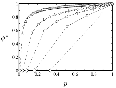
Figure 5: Bifurcation points for $\bar{d^{\ast}}>1$, ${\phi^{\ast}}>1$, and $r=1$, determined numerically using equations Eq. (13) and Eq. (14). The data shown are for $T=3$ ($\bigcirc$), $T=6$ ($\Box$), $T=12$ ($\triangleleft$), $T=24$ ($\triangleright$), and $T=96$ ($\vartriangle$). The solid lines guide the eye for the range $\bar{d^{\ast}}=2$ to $\bar{d^{\ast}}=T-1$ with $\bar{d^{\ast}}$ increasing with $p_{b}$. The dashed lines connect to the transcritical bifurcation points ($\diamond$) observed for $\bar{d^{\ast}}=1$. Note that no bifurcations occur when $\bar{d^{\ast}}=T>1$ (the sole fixed point is ${\phi^{\ast}}=1$ when $p=1$) and when $\bar{d^{\ast}}=T=1$ (the fixed points lie along the line $p=1$ and $0\leq\phi\leq 1$).

As with epidemic threshold models, the analysis for critical mass dynamics can be generalized to include a non-trivial recovery rate $r<1$. Now, however, we are unable to find a closed-form expression for the fixed points for general $T$ and $\bar{d^{\ast}}$. The difficulty in making such a computation lies in finding an expression for the number of individuals whose dose counts are below threshold but are still infected since they have not yet recovered. For the $\bar{d^{\ast}}=1$ case, this was straightforward since the only way to stay below threshold was to experience a sequence of null exposures. Nevertheless, for $r<1$, we can formally modify the expression for ${\phi^{\ast}}$ given in Eq. (13):

$${\phi^{\ast}}=\Gamma(p,{\phi^{\ast}};r,T)+\sum_{i=\bar{d^{\ast}}}^{T}\binom{T}{i}(p{\phi^{\ast}})^{i}(1-p{\phi^{\ast}})^{T-i},$$ (15)

where the additional term $\Gamma(p,{\phi^{\ast}};r)$ accounts for the proportion of below threshold individuals who have not yet recovered. For small values of $T$ and $\bar{d^{\ast}}$, exact expressions for $\Gamma(p,{\phi^{\ast}};r)$ can be derived and then ${\phi^{\ast}}$ can be solved for numerically. In Appendix B, we consider two special cases, $\bar{d^{\ast}}=2$ for $T=2$ and $T=3$, that illustrate the process of constructing expressions for $\Gamma(p,{\phi^{\ast}};r)$. These results allow us to explore the movement of the fixed points with decreasing $r$. Figures 6 A and B show comparisons over a range of $r$ between the solutions of Eq. (15) and simulations for $T=2$ and $T=3$ respectively, confirming that the agreement is excellent.

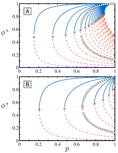
Figure 6: A: Theory versus simulation for $T=3$, $\bar{d^{\ast}}=2$, and varying $r$. Solid lines represent theoretically derived stable fixed points, dashed lines represent unstable ones, and the squares indicate bifurcation points (using Eqs. (15) and (B)). From left to right, we have $r=0.01,0.05,0.10,0.15,\ldots,1.00$. The circles correspond to simulation data for the case $r=0.2$ and matches the theoretical curves. B: Theoretical fixed point curves for $T=2$, $\bar{d^{\ast}}=2$, and varying $r$. Bifurcations appear for $r<0.3820\pm 0.0001$. Otherwise, $(p,{\phi^{\ast}})=(1,1)$ is the only fixed point of the system with ${\phi^{\ast}}>0$. The values of $r$ are as per the $T=3$ case in A. Circles correspond to simulation results for $r=0.1$. For all values of $r$, both of the above systems possess a line of stable fixed points described by $0\leq p<1$ and ${\phi^{\ast}}=0$, i.e., the $p$-axis.

IV Heterogeneous SIS contagion models

IV.1 Distributions of doses and thresholds

In real populations, both in the context of infectious diseases and also social influences, individuals evidently exhibit varying levels of susceptibility. Furthermore, contacts between infected and susceptible individuals can result in effective exposures of variable size, depending on the individuals in question, as well as the nature of their relationship and the circumstances of the contact (duration, proximity, etc.). Our homogeneity assumption of the preceding section is therefore unlikely to be justified in any real application. Furthermore, as we show below, the more general case of heterogeneous populations, while preserving much of the structure of the homogeneous case, also yields a new class of dynamical behavior; thus the inclusion of heterogeneity not only makes the model more realistic, but also provides additional qualitative insight.

While in principle all parameters in the model could be assumed to vary across the population, we focus here on two parameters—individual threshold $d^{\ast}$ and dose size $d$—which when generalized to stochastic variables, embody the variations in individual susceptibility and contacts that we wish to capture. We implement these two sources of heterogeneity as follows. In the case of thresholds, each individual is assigned a threshold drawn randomly from a specified probability distribution $g(d^{\ast})$ at $t=0$ which remains fixed for all $t$. In effect, this assumption implies that individual characteristics remain roughly invariant on the time scale of the dynamics, rather than varying from moment to moment. By contrast, in order to capture the unpredictability of circumstance, we assign dose sizes stochastically, according to the distribution $f(d)$, independent both of time and the particular individuals between whom the contact occurs.

Again considering first the more tractable $r=1$ version of the SIS model, we first examine the effect of allowing dose size $d$ to vary while holding thresholds $d^{\ast}$ fixed across the population. In the homogeneous case, $k$ exposures of a susceptible to infected individuals resulted in a dose count of $k$, but the result can be more complicated when $d$ is allowed to vary continuously. Note that $d^{\ast}$ also no longer need be an integer. First, we calculate the probability that a threshold will be exceeded by $k$ doses. As the distribution of dose size is now some arbitrary function $f$, we have that the probability distribution of the sum of $k$ doses is given by the $k$-fold convolution

$$\mathbf{P}\left(\textstyle{\sum_{j=1}^{k}d_{j}=d}\right)=f\ast f\ast\cdots\ast f(d)=f^{k\star}(d).$$ (16)

The probability of exceeding $d^{\ast}$ is then

$$\mathbf{P}\left(\textstyle{\sum_{j=1}^{k}d_{j}\geq d^{\ast}}\right)=\int_{d=d^{\ast}}^{\infty}\mbox{d}d\,f^{k\star}(d).$$ (17)

Since, for $r=1$, individuals are only infected when their dose count exceeds their threshold, we have that the steady-state fraction infected is given by

$${\phi^{\ast}}=\sum_{k=1}^{T}\binom{T}{k}(p{\phi^{\ast}})^{k}(1-p{\phi^{\ast}})^{T-k}\int_{d=d^{\ast}}^{\infty}\mbox{d}d\,f^{k\star},$$ (18)

where we have averaged over all possible ways an individual may experience $1\leq k\leq T$ exposures in $T$ interactions.

Next, in order to account for any variation $d^{\ast}$, we must incorporate another layer of averaging into Eq. (18) as follows:

$${\phi^{\ast}}=$$

$$\int_{0}^{\infty}\!\!\!\mbox{d}d^{\ast}g(d^{\ast})\sum_{k=1}^{T}\binom{T}{k}(p{\phi^{\ast}})^{k}(1-p{\phi^{\ast}})^{T-k}\int_{d=d^{\ast}}^{\infty}\!\!\!\mbox{d}d\,f^{k\star}(d),$$

$$=\sum_{k=1}^{T}\binom{T}{k}(p{\phi^{\ast}})^{k}(1-p{\phi^{\ast}})^{T-k}P_{k},$$ (19)

where $P_{k}$ is defined by Eq. (3). An important insight that can be derived immediately from Eq. (IV.1) is that all information concerning the distributions of dose sizes and thresholds is expressed via the $\{P_{k}\}$; hence the details of the functions $f$ and $g$ are largely unimportant. In other words, many pairs of $f$ and $g$ can be constructed to give rise to the same $\{P_{k}\}$ and hence the same fixed points. For example, any desired $\{P_{k}\}$ can be realized by a uniform distribution of unit doses $f(d)=\delta(d-1)$, along with a discrete distribution of thresholds

$$g(d^{\ast})=P_{1}\delta(d^{\ast}-1)+\sum_{k=1}^{T-1}(P_{k+1}-P_{k})\delta(d^{\ast}-k-1).$$ (20)

We observe that for the homogeneous case where doses and thresholds are fixed at $1$ and $\bar{d^{\ast}}$ respectively [i.e., $f(d)=\delta(d-1)$ and $g(d^{\ast})=\delta(d^{\ast}-\bar{d^{\ast}})$], we have $f^{k\star}(d)=\delta(d-k)$ and the expression for $P_{k}$ [Eq. (3)] simplifies to $P_{k}=0$ if $k<\bar{d^{\ast}}$ and $P_{k}=1$ if $k\geq\bar{d^{\ast}}$. Substituting these conditions into Eq. (IV.1), we recover our previous expression Eq. (13) for the $r=1$ homogeneous case.

IV.2 Universal classes of contagion

In the homogeneous version of the model, we determined the existence of two classes of dynamics—epidemic threshold and critical mass—with the former arising whenever $\bar{d^{\ast}}=1$, and the latter when $\bar{d^{\ast}}\geq 2$. In other words, in homogeneous populations, the condition for differentiating between one class of behavior and another is a discrete one. Once heterogeneity is introduced, however, we observe a smooth transition between epidemic threshold and critical mass models governed by a continuous adjustment of the distributions $f$ and $d$ (or equivalently the $\{P_{k}\}$). One consequence of this now-continuous transition is the appearance of an intermediate class of models, which we call vanishing critical mass (see Fig. 7). As with pure critical mass models, this new class is characterized by a saddle-node bifurcation, but now the lower unstable branch of fixed points crosses the $p$-axis at $p_{c}$; in other words, the required critical mass “vanishes.” The collision of the unstable branch of the saddle node bifurcation with the horizontal axis also effectively reintroduces a transcritical bifurcation, in the manner of epidemic threshold models. However, the transcritical bifurcation is different from the one observed in epidemic threshold models because the rising branch of the bifurcation has negative, rather than positive, slope and comprises unstable, rather than stable, fixed points. Vanishing critical mass dynamics are therefore qualitatively distinct from both previously identified classes of behavior, exhibiting important properties of each: for $p<p_{c}$, they behave like critical mass models; and for $p>p_{c}$, they behave like epidemic threshold models, in the sense that an infinitesimal initial seed can spread.

Our generalized model therefore exhibits behavior that falls into one of only three universal classes: class I (epidemic threshold), class II (vanishing critical mass), and class III (critical mass). As we show below, more complicated fixed point curves exist (i.e., curves possessing two or more saddle-node bifurcation points) but nevertheless belong to one of these three universal classes, since together they include all possible behaviors of the fixed point curves near $p=p_{c}$.

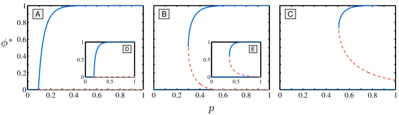
Figure 7: Fixed point curves for the three main classes of contagion models produced by the model, along with transitions between classes. All curves are determined by numerical solution of Eq. (IV.1) with an error tolerance of $10^{-10}$. Here, $T=12$, individual doses are lognormally distributed with mean 1 and a variance of $0.6$ for the underlying normal distribution, and thresholds are homogeneously distributed with $g(d^{\ast})=\delta(d^{\ast}-\bar{d^{\ast}})$. The main plots correspond to (A) $\bar{d^{\ast}}=0.4$ (class I), (B) $\bar{d^{\ast}}=1.5$ (class II), and (C) $\bar{d^{\ast}}=3$ (class III). The insets plots (D) and (E) respectively show fixed point curves for models at the class I-class II transition (i.e., when $P_{1}=P_{2}/2$ which occurs when $\bar{d^{\ast}}=0.8600\ldots$) and the class II-class III transition (i.e., when $p_{c}=1$ which occurs when $\bar{d^{\ast}}=1.9100\ldots$). In all plots except (E), the intersection between the fixed point curve and the $p$-axis is a transcritical bifurcation. In plots (B), (C), and (E), the second bifurcation is a saddle-node bifurcation.

In addition to identifying three universal classes of behavior, it is also possible to specify the conditions that govern into which class any particular choice of model parameters will fall. For $r=1$, we can calculate when the transitions between universal classes occur in terms of the parameters of interest; that is, the $\{P_{k}\}$ (viz $f$ and $g$) and $T$. This exercise amounts to locating the transcritical bifurcation and determining when it collides with the saddle-node bifurcation. To locate the transcritical bifurcation, we examine the fixed point equation as ${\phi^{\ast}}\rightarrow 0$. Since, from Eq. (IV.1),

$${\phi^{\ast}}=Tp{\phi^{\ast}}P_{1}+O({\phi^{\ast}}^{2}),$$ (21)

we have

$$p_{c}=\frac{1}{TP_{1}}.$$ (22)

The position of the transcritical bifurcation is therefore determined by the memory length $T$ and the fraction of individuals who are typically infected by one exposure, $P_{1}$. We see immediately that the transition between class II and class III contagion models occurs when $p_{c}=1$; that is, when

$$P_{1}=1/T.$$ (23)

Recalling the homogeneous case, we see that when $\bar{d^{\ast}}=d=1$, $P_{1}=1$, giving $p_{c}=1/T$ as before. It necessarily follows that when $\bar{d^{\ast}}>d=1$, $P_{1}=0$ and therefore $p_{c}=\infty$, thus confirming our earlier finding that the homogeneous model with $\bar{d^{\ast}}>1$ is always in the pure critical mass class (i.e., the lower, unstable fixed point curve of the saddle node bifurcation must have ${\phi^{\ast}}>0$ for all $p_{b}\leq p\leq 1$ since it only reaches ${\phi^{\ast}}=0$ in the limit $p\rightarrow\infty$). We also see that technically all models possess a transcritical bifurcation somewhere along the $p$-axis, even though it may be located beyond $p_{c}>1$ (when $P_{1}=0$, it lies at $p_{c}=\infty$).

In order to locate the transition between classes I and II, we determine when the transcritical and saddle-node bifurcations are coincident, i.e., when $\mbox{d}{\phi^{\ast}}/\mbox{d}p=\infty$ at $(p,{\phi^{\ast}})=(p_{c},0)$. In other words, we calculate when the fixed point curve emanating from $p=p_{c}$ is at the transition between having a large positive slope (class I) and a large negative slope (class II). We find the condition for this first transition is

$$P_{1}=P_{2}/2,$$ (24)

where details of this calculation are provided in Appendix C.

The condition of Eq. (24) is a statement of linearity in the $\{P_{k}\}$, though importantly only for $k=1$ and $k=2$. Providing $p_{c}<1$, if $P_{1}>P_{2}/2$ (i.e., sublinearity holds) a contagion model is class I whereas if $P_{1}>P_{2}/2$ (i.e., superlinearity holds) it is class II. This condition means that class II contagion models arise when, on average, two doses are more than twice as likely as one dose to cause infection.

When this condition is satisfied exactly, the system’s phase transition is a continuous one as per those of class I, but of a different universality class: class I systems exhibit a linear scaling near the critical point whereas the scaling when $P_{1}=P_{2}/2$ is ${\phi^{\ast}}\propto(p-p_{c})^{1/2}$ (in Appendix C, we show that a sequence of increasingly specific exceptions to this scaling exist depending on the extent of linearity present in the $\{P_{k}\}$).

Thus, for $r=1$, the condition that determines whether a given system is described by an epidemic threshold model, a critical mass model, or a member of the intermediate class of vanishing critical mass models, depends only on $T$, $P_{1}$, and $P_{2}$—a surprising result given that Eq. (IV.1) clearly depends on all the $\{P_{k}\}$. A summary of the three basic system types, the transitions between them, and the accompanying conditions is given in Table 2.

Model class:	Conditions:
I: Epidemic threshold	$P_{1}>P_{2}/2$ and $P_{1}>1/T$
I-II transition	$P_{1}=P_{2}/2$ and $P_{1}>1/T$
II: Partial critical mass	$P_{1}<P_{2}/2$ and $P_{1}>1/T$
II-III transition	$P_{1}<P_{2}/2$ and $P_{1}=1/T$
Pure critical mass	$P_{1}<P_{2}/2$ and $P_{1}<1/T$

Table 2: Summary of basic states of the $r=1$, heterogeneous version of model along with the corresponding parameter ranges. The $P_{k}$ quantities depend on the distributions of dose size and individual thresholds, and are given in Eq. (3).

For $r<1$, the position of the transcritical bifurcation, Eq. (25), generalizes in the same manner as Eq. (12). We find

$$p_{c}=\frac{1}{P_{1}(T+\tau)},$$ (25)

where we recall that $\tau=1/r-1$. As we will see in Section V, the above statement is also true for $\rho<1$ and thus stands as a completely general result for the model. We therefore have a condition for the transition between class II and class III contagion models for a given $T$ and $r$, analogous to that for the $\rho=1$ case in Eq. (23): $P_{1}=1/(T+\tau)$. For $r<1$, the condition for the transition between class I and class II contagion models is more complicated both in derivation and form. We observe that as $r$ is decreased, class III models must at some point transition to class II models and class II models will eventually become class I models, where we can determined the former tranisition by setting $p_{c}=1$ in Eq. (25) and solving for $r$:

$$r=\frac{P_{1}}{1+P_{1}-P_{1}T}.$$ (26)

In Eq. (26) we have assumed $P_{1}>0$ and $P_{1}T<1$, since the $r=1$ limit is, by assumption, a class III contagion model. Fig. 8 presents an example of a model transitioning from Class III through Class II to Classs I.

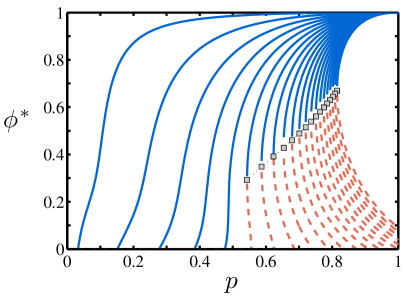
Figure 8: Example of transitions between all three classes of contagion models occurring as the probability of recovery $r$ changes. Shown are theoretically derived fixed point curves for a range of $r$ for $T=3$ and a heterogeneous population with threshold distribution $g(d^{\ast})=0.3\delta(d^{\ast}-1)+0.7\delta(d^{\ast}-2)$. From left to right, the curves correspond to $r=0.01,0.05,0.10,0.15,\ldots,1.00$. Solid lines indicate stable fixed points, dashed lines unstable ones, and the squares mark saddle-node bifurcation points. The $p$-axis is a line of fixed points, and for all fixed point curves, dashed lines indicate unstable fixed points and solid lines stable ones. For $r>0.75$, the system belongs to class III (see Eq. (26)). Fixed points lying on the $p$-axis are not indicated in the plot. For each instance of the model, points on the $p$-axis to the left of $p_{c}$ (the intercept of the non-zero fixed point curve with the $p$-axis) are stable and points to the right are unstable. The expression used here to determine the fixed points is formed by appropriately weighting a combination of Eqs. (10), (15), and (B).

IV.3 Composite classes of dynamics

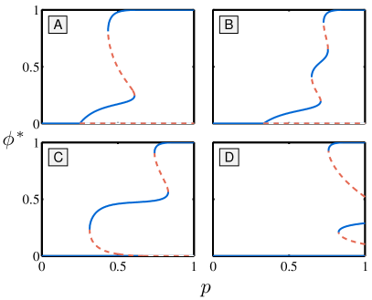
Figure 9: Fixed point curves involving multiple bifurcations. In all four examples, $T=20$ , $r=1$, and dose size is uniformly held at unity. The different curves are obtained by adjusting the threshold distribution $g$ which in turn leads to changes in the $\{P_{k}\}$ [see Eq. (3)]. The curves correspond to (A) $g(d)=0.2\delta(d-1)+0.8\delta(d-6)$; (B) $g(d)=0.15\delta(d-1)+0.4\delta(d-5)+0.45\delta(d-12)$; (C) $g(d)=0.075\delta(d-1)+0.4\delta(d-2)+0.525\delta(d-12)$; and (D) $g(d)=0.3\delta(d-3)+0.7\delta(d-12)$. Note that example (D) consists of two separate fixed point curves. The curves were found numerically by solving for $p({\phi^{\ast}})$ using Eq. (IV.1). Solid and dashed lines indicate stable and unstable fixed points respectively.

Although our main results (three universal classes of behavior and the conditions that govern the transitions between the three) involve examples of contagion models with at most two bifurcations, other more complicated kinds of equilibrium behavior are possible. Fig. 9 shows four examples of what can happen for particular distributions of $d^{\ast}$ across the population. In each example, $T=20$ and $r=1$, all doses are of unit size, and the population is divided into either two or three subpopulations with distinct values of $d^{\ast}$. The main features of each system are captured by the number and locations of the saddle-node bifurcations. As was the case for the homogeneous model [see Eq. (14)], we are able to find an expression for $z=p_{b}{\phi_{b}^{\ast}}$:

$$0=\sum_{k=1}^{T}\binom{T}{k}P_{k}z^{k-2}(1-z)^{T-k-1}[k-1-z(T-1)],$$ (27)

where the details of this calculation are provided in Appendix A. In principle, Eq. (27) could be analyzed to deduce which $\{P_{k}\}$ (and hence which $f$ and $g$) lead to what combination of bifurcations. While substantially more complicated, and thus beyond the scope of this paper, such a classification scheme would be a natural extension of our present delineation of the model into three universal classes of contagion models, based on the behavior near $p=p_{c}$. One simple observation, however, is that Eq. (27) is a polynomial of order $T-2$ and hence a maximum of $T-2$ saddle-node bifurcations may exist. From our investigations this outcome seems unlikely as nearby bifurcations tend to combine with or overwhelm one another; in other words, subpopulations with sufficiently distinct $d^{\ast}$ are required to produce systems with multiple saddle-node bifurcations. Furthermore, the distribution of dose sizes $f$ seems unlikely to be multimodal for real contagious influences or entities, and the way it enters into the calculation of the $\{P_{k}\}$ [Eq. (3)] reduces its effect in producing complicated systems. Thus, the number of distinct bifurcations is limited and strong multimodality in the threshold distribution $g$ appears to be the main mechanism for producing systems with more than one saddle node bifurcation. As a first step in this extended analysis of the model, we derive in Appendix A the condition for the appearance of two saddle-node bifurcations (i.e., one forward and one backward).

V SIRS and SIR Contagion Models

As mentioned in section II, the SIS class of behavior that we have analyzed exclusively up to now is a somewhat special case of the general contagion process as it assumes that recovered individuals instantly become re-susceptible. This assumption renders the SIS case particularly tractable, and we have taken advantage of this fact in the preceding sections to make some headway in understanding the full range of equilibrium behavior of the model. However, it remains the case that very few, if any, infectious diseases could be considered to obey true SIS-type dynamics, as almost all recovery from infection tends to be associated with some finite period of immunity. Any purportedly “general” model of contagion ought therefore to be analyzed in a wider domain of the associated removal period, and any corresponding classes of behavior labeled “universal” ought to withstand the introduction of at least some period of immunity to re-infection. Thus motivated, we now extend our previous analysis to systems where individuals experience temporary (SIRS, $0<\rho<1$) or permanent removal (SIR, $\rho=0$). We present some preliminary results for each of these cases in turn, relying now exclusively on numerical simulation.

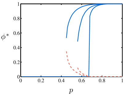
Figure 10: The effect of reducing $\rho$ (the probability of an immune individual becoming susceptible) for a contagion model that is class II when $\rho=1$. Here, $N=10^{5}$, $T=6$, $r=1$, dose sizes are fixed at unity, and $g(d^{\ast})=0.25\delta(d^{\ast}-1)+0.75\delta(d^{\ast}-2)$. From left to right, the plots correspond to $\rho=1$, $0.15$, and $0.09$. In all cases, $p_{c}$, the position of the $p$-axis intercept, is independent of $\rho$. Apart from the intercept at $p=p_{c}$ and the point $(p,{\phi^{\ast}})=(1,1)$, all other points of the curve move to the right as $\rho$ decreases. Consequently, as $\rho$ is reduced, all class II contagion models will at some point become members of class I. Contagion models in class I and class III remain unchanged in their nature. In finding the upper stable branch of ${\phi^{\ast}}(p)$, all individuals are initially infected. A binary search is then used to detect the position of the lower unstable branch.

For SIRS contagion, we observe that the position of the transcritical bifurcation $(p_{c},0)$ does not change as $\rho$ is reduced from 1; however, all non-zero fixed points move in the positive $p$ direction. Because they remain in the removed state for a longer time, individuals in systems with lower $\rho$ spend relatively less time infected than those in systems with higher $\rho$ (this is in contrast to the effect of reducing $r$, which prolongs the time individuals are infected, thereby causing fixed points to move in the negative $p$ direction). Thus, contagion models belonging to class I and class III in the $\rho=1$ special case remain in their respective classes as $\rho$ decreases. However, as shown in Fig. 10, class II models will transition to class I for some $\rho<1$.

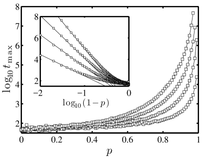
Figure 11: Time taken for an initially universal infection to die out in the SIR case ($\rho=0$). Moving from bottom to top in both plots, $T=3$, 4, 5, and 6. The model parameters used here are $d^{\ast}=1$, unit dose size, $r=0.2$, and population size $N=10^{4}$. For all systems, $p=\phi=1$ is a fixed point and hence $t_{\rm max}=\infty$ at $p=1$. The main plot shows the rapid increase in $t_{\rm max}$ for $p\rightarrow 1$. The inset shows the behavior of $t_{\rm max}$ as a function of $(1-p)$ as plotted on a double logarithmic scale. The lines have slopes of $-(T-1)$ indicating that infections are strongly persistent with $t_{\rm max}\propto(1-p)^{-(T-1)}$.

For the SIR version of the model, recovered individuals cannot return to the susceptible state, and no fraction of the population remains infected in the infinite time limit; hence we can no longer speak of non-zero fixed point curves, and the fraction of individuals infected and recovered, $\phi(t)$ and $R(t)$, become the relevant objects of study. Some defining quantities are then the maximum fraction of the population infected at any one time, $\max_{t}\phi(t)$, the fraction eventually infected, $1-\phi(\infty)-R(\infty)$, and the relaxation time required for the epidemic to die out. We focus on the latter here which we denote by $t_{\rm max}$.

We observe that when individuals possess a memory of doses (i.e., $T>1$), $t_{\rm max}$ diverges as $p\rightarrow 1$. Figure 11 shows $t_{\rm max}(p)$ for four sample systems with $T=3$, 4, 5, and 6. We find the divergence of $t_{\rm max}$ near $p=1$ to be well approximated by

$$t_{\rm max}\propto(1-p)^{-(T-1)},$$ (28)

where fits are shown in the inset of Fig. 11. Equation (28) also shows that for a fixed $p$, the relaxation time increases exponentially with length of memory $T$ for all $p$, i.e.,

$$t_{\rm max}\propto e^{\alpha T},$$ (29)

where $\alpha=-\ln{(1-p)}>0$.

Thus, when $\rho=0$, epidemics, while not ever achieving a non-zero steady state as in the $\rho>0$ case, can persist for (arbitrarily) long periods of time. The introduction of memory, which allows infected individuals to maintain their dose count above their threshold by repeatedly infecting each other, creates an SIR model with strikingly different behavior to the standard memoryless SIR model.

VI Concluding remarks

Our aim here has been to develop and analyze in detail a model of contagion that incorporates and generalizes elements of contagion models from both the social sciences and epidemiology. A key feature of the current model is that interdependencies between successive exposures are introduced in a natural way by varying the length of memory that an individual maintains of past exposures. Contagion models incorporating memory correspond to standard notions of contagion in the social sciences (although these models rarely discuss the role of memory explicitly), while memory-less contagion models correspond to traditional models of disease spreading. Our model suggests, however, that in reality these two kinds of contagion models may not be entirely distinct. We venture the possibility that some infectious diseases may spread in a fashion similar to social contagion processes. For example, two exposures to an agent sufficiently close in time may infect an individual with higher probability than would be expected if the exposures acted as independent events. The response of some individuals to allergens where separate doses accumulate in the body may be an example of a disease with memory. Although allergies are not contagious, they demonstrate that such a phenomenon is biologically plausible—a possibility that has largely remained unexamined in the microorganismal dose-response literature (haas2002, ).

The main result of our analysis is the identification of three universal classes of contagion dynamics, along with precise conditions for the transitions between these classes. Given the complexity of the model, these conditions are surprisingly simple—at least in the SIS case ($r=\rho=1$, see Table 2)—and present us with quantities such as $T$, $P_{1}$, and $P_{2}$ that may in principle be measurable for real epidemics. Furthermore, the dependence of the transition conditions only on $P_{1}$, $P_{2}$, and $T$, rather than on the full details of the underlying distributions of thresholds $(g(d^{\ast}))$ and doses $(f(d))$, suggests a new and possibly useful level of abstraction for thinking about contagious processes; that is, measuring individuals in terms of their dose-response and characterizing a population in terms of its $\{P_{k}\}$.

For the more complicated and general cases of $r<1$ (finite recovery period) and $\rho<1$ (finite immunity period), we have confirmed that the same basic three-class structure persists, and determined the position of the transcritical bifurcation $p_{c}$, Eq. (25), that is one of the two quantities needed to specify the conditions for transitioning between classes. The other condition, derived from calculating the slope of the fixed point curve as it passes through the transcritical bifurcation, merits further attention. All of these conditions, however, are ultimately dependent on the distributions $f$ and $g$. Our analysis of the model suggests, for example, that composite fixed point diagrams involving more than one saddle point node can only result from multimodality in $g$, the distribution of thresholds. Exactly how the details of these two distributions affect $P_{1}$ and $P_{2}$ would be worth further investigation.

Our model suggests that some epidemics may be prevented or enabled with slight changes in system parameters (if feasible). For example, knowing that a potentially contagious influence belongs to class II and that $p$ is just below $p_{c}$ would indicate that by increasing inherent infectiousness (i.e., $p$) or by creating a sufficiently large enough base of infected individuals, the contagion could be kicked off with potentially dramatic results. Alternatively, by increasing $r$ or reducing $T$ or $\rho$, the possibility of undesirable epidemics may be reduced, as for all these adjustments fixed point curves are generally moved in the direction of higher values of $p$.

Finally, we have focused exclusively in this paper on a mean field analysis of the model, which is to say, we have made the standard assumption that individuals in a population mix uniformly and at random. A natural generalization would be to consider the model’s behavior for a networked population of individuals. Other simulation possibilities would be to consider distributions of $T$, $p$, $r$, and $\rho$. Finally, additional technical investigation of this model would also include analysis of the closed-form expression for saddle-node bifurcations given in Eq. (27), and a derivation of analytic expressions for the model when $\rho<1$ for small $T$ and $d^{\ast}$. We hope that our preliminary investigations into this interesting and reasonably general class of contagion models will stimulate other researchers to pursue some of these extensions.

Appendix A Conditions for existence of saddle-node bifurcation

In Eq. (27), we provided a closed form expression for $z=p_{b}{\phi_{b}^{\ast}}$ where $(p_{b},{\phi_{b}^{\ast}})$ is the location of a saddle-node bifurcation. This expression pertains to the heterogeneous version of the model for $r=\rho=1$ [the homogeneous version is given in Eq. (14)]. As noted in the main text, this equation has up to $T-2$ solutions, depending on the form of the $\{P_{k}\}$. In this Appendix, we derive Eq. (27) and also find a criterion for the appearance of two saddle-node bifurcations. All calculations revolve around determining when the slope of the fixed point curve ${\phi^{\ast}}(p)$ becomes infinite, or, equivalently, finding when $\mbox{d}p/\mbox{d}{\phi^{\ast}}=0$.

Our starting point is Eq. (IV.1), the general closed form expression for ${\phi^{\ast}}$ as a function of $p$, from which we can calculate $\mbox{d}p/\mbox{d}{\phi^{\ast}}$. We rewrite Eq. (IV.1) as

$$u(p,{\phi^{\ast}}) = -{\phi^{\ast}}+\sum_{k=1}^{T}\binom{T}{k}P_{k}(p{\phi^{\ast}})^{k}(1-p{\phi^{\ast}})^{T-k},$$ (30)

$$= {\phi^{\ast}}\left[-1+p\sum_{k=1}^{T}\binom{T}{k}P_{k}(p{\phi^{\ast}})^{k-1}(1-p{\phi^{\ast}})^{T-k}\right],$$

$$= {\phi^{\ast}}\,U(p,{\phi^{\ast}}),$$

with the requirement $u(p,{\phi^{\ast}})=0$.

We show that we can use the function $U$ instead of $u$ to find $\mbox{d}p/\mbox{d}{\phi^{\ast}}$ when ${\phi^{\ast}}\neq 0$. Differentiating $u(p,{\phi^{\ast}})=\phi U(p,{\phi^{\ast}})=0$ with respect to ${\phi^{\ast}}$, we have

$$\frac{\partial u}{\partial{\phi^{\ast}}}+\frac{{\rm d}p}{{\rm d}{\phi^{\ast}}}\frac{\partial h}{\partial p}=U+{\phi^{\ast}}\frac{\partial U}{\partial{\phi^{\ast}}}+{\phi^{\ast}}\frac{{\rm d}p}{{\rm d}{\phi^{\ast}}}\frac{\partial U}{\partial p}=0.$$ (31)

Again, since $u(p,{\phi^{\ast}})={\phi^{\ast}}U(p,{\phi^{\ast}})=0$, we have $U(p,{\phi^{\ast}})=0$ when ${\phi^{\ast}}\neq 0$. When we also require $\mbox{d}p/\mbox{d}{\phi^{\ast}}=0$ (i.e., the chief condition for a saddle-node bifurcation point), Eq. (31) reduces to

$$\frac{\partial U}{\partial{\phi^{\ast}}}=0,$$ (32)

and so we may find solutions of $\partial U/\partial{\phi^{\ast}}=0$ instead of $\partial u/\partial{\phi^{\ast}}=0$. The benefit of making this observation is that we find $\partial U/\partial{\phi^{\ast}}$ can be expressed in terms of a single variable ($z=p_{b}{\phi_{b}^{\ast}}$), allowing for simpler analytical and numerical examination (recall that $(p_{b},{\phi_{b}^{\ast}})$ denotes the position of a saddle-node bifurcation). Returning to the definition of $U$ given in Eq. (30), we find

$$\frac{\partial U}{\partial{\phi^{\ast}}}=\sum_{k=1}^{T}\binom{T}{k}P_{k}p^{k}(k-1)({\phi^{\ast}})^{k-2}(1-p{\phi^{\ast}})^{T-k}$$ (33)

$$+\sum_{k=1}^{T}\binom{T}{k}P_{k}p^{k}({\phi^{\ast}})^{k-1}(T-k)(-p)(1-p{\phi^{\ast}})^{T-k-1}$$

$$+\frac{{\rm d}p}{{\rm d}{\phi^{\ast}}}\left(\ldots\right).$$

Since we require $\mbox{d}p/\mbox{d}{\phi^{\ast}}=0$, the above simplifies to

$$\frac{\partial U}{\partial{\phi^{\ast}}}=\sum_{k=1}^{T}\binom{T}{k}P_{k}p^{k}({\phi^{\ast}})^{k-2}(1-p{\phi^{\ast}})^{T-k-1}$$ (34)

$$\times\left[(k-1)(1-p{\phi^{\ast}})-p{\phi^{\ast}}(T-k)\right].$$

Setting $\partial U/\partial{\phi^{\ast}}=0$ and removing a factor of $p^{2}$, we find the positions of all saddle-node bifurcation points satisfy

$$0=\sum_{k=1}^{T}\binom{T}{k}P_{k}z^{k-2}(1-z)^{T-k-1}[k-1-z(T-1)],$$ (35)

where $z=p_{b}{\phi_{b}^{\ast}}$. Upon solving Eq. (35) for $z$ (where for all nontrivial solutions, we require $0<z<1$), Eq. (IV.1) can then be used to find ${\phi_{b}^{\ast}}$ (since it expresses ${\phi_{b}^{\ast}}$ as a function of $z$) and hence $p_{b}$.

In order to determine whether a bifurcation is forward or backward facing (by forward facing, we mean branches emanate from the bifurcation point in the direction of the positive $p$-axis), we need to compute $\mbox{d}^{2}p/\mbox{d}{{\phi^{\ast}}}^{2}$, and examine its sign. (When $\mbox{d}^{2}p/\mbox{d}{{\phi^{\ast}}}^{2}=0$, two saddle-node bifurcations points are coincident, one forward and one backward facing.) If the $\{P_{k}\}$ are parametrized in some fashion (i.e., $f$ and/or $g$ are parametrized), then we can determine the relevant parameter values at which pairs of bifurcations appear. We compute an expression for $\mbox{d}^{2}p/\mbox{d}{{\phi^{\ast}}}^{2}$ as follows.

Differentiating Eq. (31) with respect to ${\phi^{\ast}}$, we have

$$\frac{{\rm d}^{2}u}{{\rm d}{{\phi^{\ast}}}^{2}}=2\frac{{\rm d}U}{{\rm d}{\phi^{\ast}}}+{\phi^{\ast}}\frac{{\rm d}^{2}U}{{\rm d}{{\phi^{\ast}}}^{2}}=0.$$ (36)

We already have $\mbox{d}U/\mbox{d}{\phi^{\ast}}=\partial U/\partial{\phi^{\ast}}+\mbox{d}p/\mbox{d}{\phi^{\ast}}\partial U/\partial p=0$, and so Eq. (36) now gives

$$\frac{{\rm d}^{2}U}{{\rm d}{{\phi^{\ast}}}^{2}}=0.$$ (37)

Expanding this, we have

$$0=\frac{\partial^{2}U}{{\partial{\phi^{\ast}}}^{2}}+\frac{{\rm d}p}{{\rm d}{\phi^{\ast}}}\frac{\partial^{2}U}{\partial p\partial{\phi^{\ast}}}+\frac{{\rm d}^{2}p}{{\rm d}{{\phi^{\ast}}}^{2}}\frac{\partial U}{\partial p}+\frac{{\rm d}p}{{\rm d}\phi}\frac{\mbox{d}missing}{\mbox{d}p}\frac{\partial U}{\partial p}.$$ (38)

The second and fourth terms on the right hand disappear since $\mbox{d}p/\mbox{d}{\phi^{\ast}}=0$, leaving

$$0=\frac{\partial^{2}U}{{\partial{\phi^{\ast}}}^{2}}+\frac{{\rm d}^{2}p}{{\rm d}{{\phi^{\ast}}}^{2}}\frac{\partial U}{\partial p}.$$ (39)

Upon rearrangement, we have

$$\frac{{\rm d}^{2}p}{{\rm d}{{\phi^{\ast}}}^{2}}=-\frac{\partial^{2}U/\partial{{\phi^{\ast}}}^{2}}{\partial U/\partial p}.$$ (40)

We first compute $\partial U/\partial p$. With $U$ as defined in Eq. (30), we see that

$$\frac{\partial U(p,{\phi^{\ast}})}{\partial p}=\frac{\partial}{\partial p}\frac{1}{{\phi^{\ast}}}\sum_{k=1}^{T}\binom{T}{k}P_{k}(p{\phi^{\ast}})^{k}(1-p{\phi^{\ast}})^{T-k},$$ (41)

$$= \frac{\partial}{\partial p{\phi^{\ast}}}\sum_{k=1}^{T}\binom{T}{k}P_{k}(p{\phi^{\ast}})^{k}(1-p{\phi^{\ast}})^{T-k},$$

$$= \frac{\partial}{\partial z}\sum_{k=1}^{T}\binom{T}{k}P_{k}z^{k}(1-z)^{T-k},$$

$$= \sum_{k=1}^{T}\binom{T}{k}P_{k}z^{k}(1-z)^{T-k-1}[k(1-z)-(T-k)z],$$

$$= \sum_{k=1}^{T}\binom{T}{k}P_{k}z^{k}(1-z)^{T-k-1}[k-Tz].$$

Using Eqs. (30) and (35) (i.e., that we are at a bifurcation point), the above yields

$$\frac{\partial U(p,{\phi^{\ast}})}{\partial p}=\frac{1}{p}.$$ (42)

Using this result, Eq. (40) becomes

$$\frac{{\rm d}^{2}p}{{\rm d}{{\phi^{\ast}}}^{2}}=-p\frac{\partial^{2}U}{{\partial{\phi^{\ast}}}^{2}}.$$ (43)

Next, we find

$$\frac{\partial^{2}U}{{\partial{\phi^{\ast}}}^{2}}=\sum_{k=1}^{T}\binom{T}{k}P_{k}z^{k-3}(1-z)^{T-k-2}\times$$

$$[(k-1)(k-2)-2z(k-1)(T-2)+z^{2}(T-1)(T-2)].$$

As stated above, if the $\{P_{k}\}$ are parametrized in some way, and we are interested in finding at what parameter values two bifurcations appear and begin to separate, then we need to determine when $\partial U/\partial{\phi^{\ast}}=0$ [Eq. (35)] and when $\partial^{2}U/\partial{{\phi^{\ast}}}^{2}=0$ [Eq. (A)].

If however the $\{P_{k}\}$ are fixed and we want to find all bifurcation points along with whether they are forward or backward bifurcations, then we can check the latter by finding the sign of $\mbox{d}^{2}p/\mbox{d}{{\phi^{\ast}}}^{2}=0$ [Eq. (43)]. Further analysis of these equations may be possible to find conditions on $f$ and $g$, and thereby the $\{P_{k}\}$, that would ensure certain types of model behavior.

Appendix B Exact solution for $r<1$, $d^{\ast}=2$, and $T=2$ and $T=3$

For $r<1$, in general we have individuals whose cumulative dose is below the threshold $\bar{d^{\ast}}$ but are still infected because they have not yet recovered. To find the proportion of individuals in this category, we must calculate $\Gamma_{m}$, the fraction of individuals whose memory count $D$ [number of successfully infecting interactions, Eq. (1)] last equaled the threshold $m$ time steps ago and has been below the threshold since then. The fraction of these individuals still infected will be $(1-r)^{m}$, i.e., those who have failed to recover at each subsequent time step. We write the proportion of infected individuals below the threshold as

$$\Gamma(p,{\phi^{\ast}};r,T)=\sum_{m=1}^{\infty}(1-r)^{m}\Gamma_{m}(p,{\phi^{\ast}};T).$$ (45)

Once $\Gamma$ in determined, a closed form expression for ${\phi^{\ast}}(p)$ is obtained by inserting $\Gamma$ into Eq. (15). To determine the $\{\Gamma_{m}\}$, we explicitly construct all allowable length $m$ sequences of $1$’s and $0$’s such that no subsequence of length $T$ has $d^{\ast}=2$ or more $1$’s. The analysis is similar for both the $T=2$ and $T=3$ cases we consider in this Appendix, and a generalization to all $T$ is possible. Below, we first show the forms of $\Gamma$ for the two cases and then provide details of the calculations involved.

For $T=3$, we obtain

$$\Gamma(p,{\phi^{\ast}};r,T)=(p{\phi^{\ast}})^{2}(1-p{\phi^{\ast}})^{2}\times$$

$$\biggl{(}1-r+\sum_{m=1}^{\infty}(1-r)^{m}\left[\chi^{(3)}_{m-1}+\chi^{(3)}_{m-2}+\right.\biggr{.}$$

$$\biggl{.}\left.2p{\phi^{\ast}}(1-p{\phi^{\ast}})\chi^{(3)}_{m-3}+p{\phi^{\ast}}(1-p{\phi^{\ast}})^{2}\chi^{(3)}_{m-4}\right]\biggr{)}$$

where $\chi^{(T)}_{m}$ is defined as

$$\chi^{(T)}_{m}(p,{\phi^{\ast}})=\sum_{k=0}^{[m/T]}\binom{m-(T-1)k}{k}(1-p{\phi^{\ast}})^{m-k}(p{\phi^{\ast}})^{k}.$$ (47)

Upon inserting $\Gamma$ into Eq. (15), we have a closed form expression for ${\phi^{\ast}}$ involving $p$ and $r$ as parameters. This expression can then be solved for numerically yielding the fixed point curves in Figure 6.

For the $T=\bar{d^{\ast}}=2$ case, we find

$$\Gamma(p,{\phi^{\ast}};r,T)=$$

$$(p{\phi^{\ast}})^{2}(1-p{\phi^{\ast}})\sum_{m=1}^{\infty}(1-r)^{m}\left[\chi^{(2)}_{m-1}+p{\phi^{\ast}}\chi^{(2)}_{m-2}\right].$$

We consider the case of $d^{\ast}=2$ and $T=3$ first. For this specification of the model, there are two ways for an individual to transition to being below the threshold, i.e., $D<d^{\ast}$. An individual must have two positive signals and one null signal in their memory and then receive a null signal while losing a positive signal out the back of their memory window. The two sequences for which this happens are

$$\{d_{n-2},d_{n-1},d_{n},d_{n+1}\}=\{1,1,0,0\}$$ (49)

and

$$\{d_{n-2},d_{n-1},d_{n},d_{n+1}\}=\{1,0,1,0\},$$ (50)

with the point of transition to being below the threshold occurring between time steps $n$ and $n+1$. The two other sequences for which a node will be above the threshold are $\{1,1,1\}$ and $\{0,1,1\}$ but neither of these can drop below the threshold of $d^{\ast}=2$ in the next time step. Both the sequences of Eqs. (49) and (50) occur with probability $(1-p{\phi^{\ast}})^{2}(p{\phi^{\ast}})^{2}$. When $m>1$, $d_{n+2}$ may be either $0$ or $1$ for the first sequence, but for the second $d_{n+2}=0$ or otherwise the threshold will be reached again:

$$\{d_{n-2},d_{n-1},d_{n},d_{n+1},d_{n+2}\}=\{1,0,1,0,0\},$$ (51)

Given these two possible starting points, we now calculate the number of paths for which $D_{t+j}$ remains below $d^{\ast}=2$ for $j=1,\ldots,m$. The structure of an acceptable sequence must be such that whenever a 1 appears, it is followed by at least two 0’s (otherwise, $d^{\ast}$ will be exceeded). We can see therefore that every allowable sequence is constituted by only two distinct subsequences: $a=\{0\}$ and $b=\{1,0,0\}$.

Our problem becomes one of counting how many ways there are to arrange a sequence of $a$’s and $b$’s given an overall sequence length $m$ and that the length of $a$ is 1 and the length of $b$ is 3.

If we fix the number of subsequences of $a$ and $b$ at $N_{a}$ and $N_{b}$ then we must have $m=N_{a}\cdot 1+N_{b}\cdot 3$. Varying $N_{b}$ from $0$ to $[m/3]$ (the square brackets indicate the integer part is taken), we have $N_{a}$ correspondingly varying from $m$ down to $m-3[m/3]$ in steps of $3$.

Next, we observe that the number of ways of arranging $N_{a}+N_{b}$ subsequences $a$ and $b$ is

$$\binom{N_{a}+N_{b}}{N_{a}}=\binom{N_{a}+N_{b}}{N_{b}}=\frac{(N_{a}+N_{b})!}{N_{a}!N_{b}!}.$$ (52)

To see this, consider a sequence of slots labeled $1$ through $N_{a}+N_{b}$. In ordering the $N_{a}$ $a$’s and $N_{b}$ $b$’s, we are asking how many ways there are to choose $N_{a}$ slots for the $a$’s (or equivalently $N_{b}$ slots for the $b$’s). We are interested in the labels of the slots but not the order that we select them so we obtain the binomial coefficient of Eq. (52).

Allowing $N_{b}$ and $N_{a}$ to vary while holding $m=N_{a}+3N_{b}$ fixed, we find the total number of allowable sequences to be

$$\sum_{N_{b}=0}^{[m/3]}\binom{N_{b}+N_{a}}{N_{b}}=\sum_{k=0}^{[m/3]}\binom{m-2k}{k},$$ (53)

where we have replaced $N_{b}$ with $k$ and $N_{a}$ with $3N_{b}-m=3k-m$. Noting that the probability of $a$ is $(1-p{\phi^{\ast}})$ and $b$ is $p{\phi^{\ast}}(1-p{\phi^{\ast}})^{2}$, the total probability $\chi^{(3)}_{m}(p,{\phi^{\ast}})$ of all allowable sequences of length $m$ for $T=3$ follows from Eq. (53):

$$\chi^{(3)}_{m}(p,{\phi^{\ast}})=\sum_{k=0}^{[m/3]}\binom{m-2k}{k}(1-p{\phi^{\ast}})^{m-k}(p{\phi^{\ast}})^{k}.$$ (54)

For general $T$, $\chi^{(T)}_{m}$ is defined by equation Eq. (47).

We must also address some complications at the start and end of allowable sequences. At the end of a sequence, we have the issue of 1’s being unable to appear because our component subsequences are $a=\{0\}$ and $b=\{1,0,0\}$. Any sequence ending in two or more $0$’s will be accounted for already but two endings we need to include are $\{d_{n+m}\}=\{1\}$ and $\{d_{n+m-1},d_{n+m}\}=\{1,0\}$. We do this for each of the two starting sequences and we therefore have six possible constructions for allowable sequences of length $m$. For the starting sequence given in Eq. (49), we have the following three possibilities for $\{d_{n-2},d_{n-1},d_{n},d_{n+1},\ldots,d_{n+m}\}$:

$$H_{1}=\{1,1,0,0,H_{m-1}^{a,b}\},$$ (55)

$$H_{2}=\{1,1,0,0,H_{m-2}^{a,b},1\},$$ (56)

and

$$H_{3}=\{1,1,0,0,H_{m-3}^{a,b},1,0\},$$ (57)

where $H_{m}^{a,b}$ is a length $m$ sequence of $a$’s and $b$’s [which as we have deduced occur with probability $\chi^{(3)}_{m}(p,{\phi^{\ast}})$]. For the starting sequence given in Eq. (51), we similarly have

$$H_{4}=\{1,0,1,0,0,H_{m-2}^{a,b}\},$$ (58)

$$H_{5}=\{1,0,1,0,0,H_{m-3}^{a,b},1\},$$ (59)

and

$$H_{6}=\{1,0,1,0,0,H_{m-4}^{a,b},1,0\}.$$ (60)

The probabilities corresponding to sequences (55) through (60) are

$${\rm Pr}(H_{1})=(p{\phi^{\ast}})^{2}(1-p{\phi^{\ast}})^{2}\chi^{(3)}_{m-1}(p,{\phi^{\ast}}),$$ (61)

$${\rm Pr}(H_{2})=(p{\phi^{\ast}})^{3}(1-p{\phi^{\ast}})^{2}\chi^{(3)}_{m-2}(p,{\phi^{\ast}}),$$ (62)

$${\rm Pr}(H_{3})=(p{\phi^{\ast}})^{3}(1-p{\phi^{\ast}})^{3}\chi^{(3)}_{m-3}(p,{\phi^{\ast}}),$$ (63)

$${\rm Pr}(H_{4})=(p{\phi^{\ast}})^{2}(1-p{\phi^{\ast}})^{3}\chi^{(3)}_{m-2}(p,{\phi^{\ast}}),$$ (64)

$${\rm Pr}(H_{5})=(p{\phi^{\ast}})^{3}(1-p{\phi^{\ast}})^{3}\chi^{(3)}_{m-3}(p,{\phi^{\ast}}),$$ (65)

and

$${\rm Pr}(H_{6})=(p{\phi^{\ast}})^{3}(1-p{\phi^{\ast}})^{4}\chi^{(3)}_{m-4}(p,{\phi^{\ast}}).$$ (66)

Summing these will give us the probability $\Gamma_{m}$ but one small correction is needed for $m=1$. By incorporating $d_{n+2}=0$ into the sequence of Eq. (51), we considered only $m\geq 2$ sequences. So we must also add in the probability of the $m=1$ sequence given in Eq. (50) which is $(p{\phi^{\ast}})^{2}(1-p{\phi^{\ast}})^{2}$. Combining this additional quantity with the probabilities in (61) through (66), we have

$$\Gamma_{m}(p,{\phi^{\ast}},3)=(p{\phi^{\ast}})^{2}(1-p{\phi^{\ast}})^{2}\times$$

$$\left[\delta_{m1}+\chi^{(3)}_{m-1}+\chi^{(3)}_{m-2}\right.$$

$$\left.+2p{\phi^{\ast}}(1-p{\phi^{\ast}})\chi^{(3)}_{m-3}+p{\phi^{\ast}}(1-p{\phi^{\ast}})^{2}\chi^{(3)}_{m-4}\right],$$

where $\delta_{ij}$ is the Kronecker delta function and we have suppressed the dependencies of the $\chi^{(3)}_{m}$ on $p$ and ${\phi^{\ast}}$. Substituting this into equation Eq. (45), we obtain Eq. (B).

The calculation for $T=2$ follows along the same lines as above. We now have $a=\{0\}$ and $b=\{1,0\}$ as our subsequences. There is only one starting sequence,

$$\{d_{n-1},d_{n},d_{n+1}\}=\{1,1,0\},$$ (68)

as well as one exceptional ending sequences, $\{d_{n+m}\}=\{1\}$. Defining

$$\chi^{(2)}_{m}=\sum_{k=0}^{[m/2]}\binom{m-k}{k}(1-p{\phi^{\ast}})^{m-k}(p{\phi^{\ast}})^{k},$$ (69)

the probability of being above the threshold and then having no reinfections may be written as

$$\Gamma_{m}(p,{\phi^{\ast}};2)=p^{2}{\phi^{\ast}}^{2}(1-p{\phi^{\ast}})\left[\chi_{m-1}^{(2)}+p{\phi^{\ast}}\chi_{m-2}^{(2)}\right].$$ (70)

Using Eq. (70) in Eq. (45) we obtain the form for $\Gamma$ given in Eq. (B).

Appendix C Transition between class I and class II contagion models

The transition between class I and class II models of contagion occurs when a saddle-node bifurcation collides with the transcritical bifurcation lying on the $p$-axis. To find this transition, we must determine when the slope of the non-zero fixed point curve at the transcritical bifurcation (i.e., at $p=p_{c}$ and ${\phi^{\ast}}=0$) becomes infinite. For the heterogeneous version of the model with $r=1$ and variable $\{P_{k}\}$, we are able to determine the behavior near $p=p_{c}$ as follows. We first rearrange the right hand side of Eq. (IV.1) to obtain a polynomial in $p{\phi^{\ast}}$:

$${\phi^{\ast}}=\sum_{k=1}^{T}\binom{T}{k}P_{k}(p{\phi^{\ast}})^{k}(1-p{\phi^{\ast}})^{T-k},$$ (71)

$$= \sum_{k=1}^{T}\binom{T}{k}P_{k}(p{\phi^{\ast}})^{k}\sum_{j=0}^{T-k}\binom{T-k}{j}(-p{\phi^{\ast}})^{j},$$

$$= \sum_{k=1}^{T}\sum_{j=0}^{T-k}\binom{T}{k}\binom{T-k}{j}P_{k}(-1)^{j}(p{\phi^{\ast}})^{k+j},$$

$$= \sum_{l=1}^{T}\sum_{k=1}^{m}\binom{T}{k}\binom{T-k}{m-k}P_{k}(-1)^{m-k}(p{\phi^{\ast}})^{m},$$

$$= \sum_{m=1}^{T}C_{m}(p{\phi^{\ast}})^{m},$$

where we have changed the summation over $j$ and $k$ to one over $m=k+j$ and $k$. The coefficients $C_{m}$ identified in the above may be written more simply as

$$C_{m}=(-1)^{m}\binom{T}{m}\sum_{k=1}^{m}(-1)^{k}\binom{m}{k}P_{k},$$ (72)

since

$$\binom{T}{k}\binom{T-k}{m-k} = \frac{T!}{k!(T-k)!}\frac{(T-k)!}{(m-k)!(T-l)!}$$ (73)

$$= \frac{T!}{m!(T-m)!}\frac{m!}{k!(l-k)!}$$

$$= \binom{T}{m}\binom{m}{k}.$$

Expanding Eq. (71) to second order about $p=p_{c}$ and ${\phi^{\ast}}=0$, and writing $\tilde{p}=p-p_{c}$, we obtain

$${\phi^{\ast}}\simeq C_{1}(\tilde{p}+p_{c}){\phi^{\ast}}+C_{2}p_{c}^{2}{\phi^{\ast}}^{2}.$$ (74)

From Eq. (72), $C_{1}=TP_{1}(=1/p_{c})$ and $C_{2}=\binom{T}{2}(-2P_{1}+P_{2})$. Using also that $p_{c}=1/(TP_{1})$, Eq. (74) then yields

$${\phi^{\ast}}\simeq\frac{C_{1}}{C_{2}p_{c}^{2}}\tilde{p}=\frac{T^{2}P_{1}^{3}}{(T-1)(P_{1}-P_{2}/2)}\tilde{p}.$$ (75)

Upon requiring $\mbox{d}{\phi^{\ast}}/\mbox{d}p=\infty$, the transition condition of Eq. (24) follows.

If $C_{2}=0$ (i.e., $P_{1}=P_{2}/2$), the above calculation is no longer valid and the system exhibits a continuous phase transition with a nontrivial exponent at $p_{c}$. More generally, when $C_{2}=C_{3}=\ldots=C_{n}=0$, we find for small ${\phi^{\ast}}$ and $\tilde{p}$ that

$${\phi^{\ast}}\simeq\frac{C_{1}}{C_{n+1}p_{c}^{n+1}}\tilde{p}^{1/n}.$$ (76)

We observe that for $C_{2}=C_{3}=\ldots=C_{n}=0$, a linearity condition in the $\{P_{k}\}$ must hold, specifically, $P_{k}=kP_{1}$ for $k=1,\ldots,n$. To show this, we rearrange the $\{C_{m}\}$ given by Eq. (72) as follows, ignoring multiplicative factors and substituting $P_{k}=kP_{1}$:

$$C_{m} \propto \sum_{k=1}^{m}(-1)^{k}\binom{m}{k}P_{k}=\sum_{k=1}^{m}(-1)^{k}\frac{m!}{(k-1)!(m-k)!}P_{1},$$ (77)

$$\propto \sum_{k=1}^{m}(-1)^{k}\frac{(m-1)!}{(k-1)!(m-k)!}\propto\sum_{k^{\prime}=0}^{m-1}(-1)^{k^{\prime}}\binom{m-1}{k^{\prime}},$$

$$= [1+(-1)]^{m-1}=0,$$

where we have shifted the index $k$ to $k^{\prime}=k-1$.

References

- (1) J. D. Murray. Mathematical Biology. Springer, New York, Third edition, 2002.
- (2) D. J. Daley and J. Gani. Epidemic modelling : an introduction. Cambridge University Press, New York, 1999.
- (3) R. M. Anderson and R. M. May. Infectious Diseases of Humans: Dynamics and Control. Oxford Univ. Press, Oxford, 1991.
- (4) F. Brauer and C. Castillo-Chávez. Mathematical Models in Population Biology and Epidemiology. Springer-Verlag, New York, 2001.
- (5) O. Diekmann and J. A. P. Heesterbeek. Mathematical Epidemiology. Wiley, New York, 2000.
- (6) H. Hethcote. The mathematics of infectious diseases. SIAM Rev., 42:599–653, 2000.
- (7) J. Coleman, H. Menzel, and E. Katz. Medical Innovations: A Diffusion Study. Bobbs Merrill, New York, 1966.
- (8) T. W. Valente. Network Models of the Diffusion of Innovations. Hampton Press, Cresskill, NJ, 1995.
- (9) E. Rogers. The Diffusion of Innovations. Free Press, New York, Fifth edition, 1995.
- (10) S. Lohmann. The dynamics of informational cascades: The Monday demonstrations in Leipzig, East Germany, 1989-91. World Politics, 47:42–101, 1994.
- (11) R. Stark. Why religious movements succeed or fail: A revised general model. Journal of Contemporary Religion, 11:133–146, 1996.
- (12) R. L. Montgomery. The Diffusion of Religions. University Press of America, Lanham, MD, 1996.
- (13) W. O. Kermack and A. G. McKendrick. A contribution to the mathematical theory of epidemics. Proc. R. Soc. Lond. A, 115:700–721, 1927.
- (14) W. Goffman and V. A. Newill. Generalization of epidemic theory: An application to the transmission of ideas. Nature, 204:225–228, 1964.
- (15) D. J. Daley and D. G. Kendall. Stochastic rumours. J. Inst. Math. Appl., 1:42–55, 1965.
- (16) F. Bass. A new product growth model for consumer durables. Manage. Sci., 15:215–227, 1969.
- (17) T. C. Schelling. Hockey helmets, concealed weapons, and daylight saving: A study of binary choices with externalities. J. Conflict Resolut., 17:381–428, 1973.
- (18) M. Granovetter. Threshold models of collective behavior. Am. J. Sociol., 83:1420–1443, 1978.
- (19) D. J. Watts. A simple model of global cascades on random networks. Proc. Natl. Acad. Sci., 99:5766–5771, 2002.
- (20) S. Bikhchandani, D. Hirshleifer, and I. Welch. A theory of fads, fashion, custom, and cultural change as informational cascades. J. Polit. Econ., 100:992–1026, 1992.
- (21) A. V. Banerjee. A simple model of herd behavior. Quart. J. Econ., 107:797–817, 1992.
- (22) S. Morris. Contagion. Rev. Econ. Stud., 67:57–78, 2000.
- (23) W. A. Brock and S. N. Durlauf. Discrete choice with social interactions. Rev. Econ. Stud., 68:235–260, 2001.
- (24) P. S. Dodds and D. J. Watts. Universal behavior in a generalized model of contagion. Phys. Rev. Lett., 92:218701, 2004.
- (25) C. N. Haas. Conditional dose-response relationships for microorganisms: Development and application. Risk Anal., 22:455–463, 2002.
- (26) S. H. Strogatz. Nonlinear Dynamics and Chaos. Addison Wesley, Reading, Massachusetts, 1994.
- (27) N. Goldenfeld. Lectures on Phase Transitions and the Renormalization Group, volume 85 of Frontiers in Physics. Addison-Wesley, 1992.
- (28) T. C. Schelling. Micromotives and Macrobehavior. Norton, New York, 1978.
- (29) K. P. Hadeler and C. Castillo-Chávez. A core group model for disease transmission. Math. Biosci., 128:41–45, 1995.
- (30) K. P. Hadeler and P. van den Driessche. Backward bifurcation in epidemic control. Math. Biosci., 146:15–35, 1997.
- (31) J. Dushoff, W. Huang, and C. Castillo-Chávez. Backwards bifurcations and catastrophe in simple models of fatal diseases. J. Math. Biol., 36:227–248, 1998.
- (32) C. M. Kribs-Zaleta and J. X. Velasco-Hernandez. A simple vaccination model with multiple endemic states. Math. Biosci., 164:183–201, 2000.
- (33) D. Greenhalgh, O. Diekmann, and M. C. M. de Jong. Subcritical endemic steady states in mathematical models for animals with infections with incomplete immunity. Math. Biosci., 165:1–25, 2000.
- (34) C. M. Kribs-Zaleta. Center manifold and normal forms in epidemic models. In C. Castillo-Chávez, S. Blower, D. Kirschner, P. van den Driessche, and A.-A. Yakubu, editors, Mathematical Approaches for Emerging and Re-emerging Infectious Diseases, An Introduction, volume 126 of IMA Series in Mathematics and Its Applications, pages 269–286. Springer-Verlag, New York, 2002.