Sparse canonical correlation analysis

Abstract

Canonical correlation analysis was proposed by Hotelling [6] and it measures linear relationship between two multidimensional variables. In high dimensional setting, the classical canonical correlation analysis breaks down. We propose a sparse canonical correlation analysis by adding $\ell_{1}$ constraints on the canonical vectors and show how to solve it efficiently using linearized alternating direction method of multipliers (ADMM) and using TFOCS as a black box. We illustrate this idea on simulated data.

1 Introduction

Correlation measures dependence between two or more random variables. The most popular measure is the Pearson’s correlation coefficient. For random variables $x,y\in\mathbb{R}$, the population correlation coefficient is defined as $\rho_{x,y}=\frac{\mathop{\rm Cov}(x,y)}{\sqrt{{\rm Var}(x)}\sqrt{{\rm Var}(y)}}$. It is of importance that the correlation takes out the variance in random variables $x$ and $y$ by dividing the standard deviation of them. We could not emphasize more the importance of this standardization, and we present two toy examples in Table 1. Clearly, $x$ and $y$ are more correlated in the left table than the right table even though the covariance between $x$ and $y$ are seemingly much smaller in the left table than that in the right table.

Covariance	$x$	$y$
$x$	0.1	0.09
$y$	0.09	0.1

and   Covariance $x$ $y$ $x$ 0.9 0.3 $y$ 0.3 0.9

Table 1: Covariance Matrix

Canonical correlation studies correlation between two multidimensional random variables. Let $x\in\mathbb{R}^{p}$ and $y\in\mathbb{R}^{q}$ be random variables, and let $\Sigma_{x}$, $\Sigma_{y}$ be covariance of $x$ and $y$ respectively, and their covariance matrix be $\Sigma_{xy}$. In simple words, it seeks linear combinations of $x$ and $y$ such that the resulting values are mostly correlated. The mathematical definition is

$$\underset{u\in\mathbb{R}^{p},v\in\mathbb{R}^{q}}{\text{maximize}}\ \ \ \frac{u^{T}\Sigma_{xy}v}{\sqrt{u^{\prime}\Sigma_{x}u}\sqrt{v^{\prime}\Sigma_{y}v)}}.$$ (1)

Solving Equation 1 is easy in low dimensional setting, i.e., $n\gg p$, because we can use change of variables: $\Sigma^{1/2}_{x}u=a$, and $\Sigma_{y}^{1/2}v=b$. Equation 1 becomes

$$\underset{a\in\mathbb{R}^{p},b\in\mathbb{R}^{q}}{\text{maximize}}\ \ \ \frac{a^{T}\Sigma_{x}^{-1/2}\Sigma_{xy}\Sigma_{y}^{-1/2}b}{\sqrt{a^{T}a}\sqrt{b^{T}b}}.$$ (2)

Solving Equation 2 is equivalent to solving singular decomposition of the new matrix $\Sigma^{-1/2}_{x}\Sigma_{xy}\Sigma_{y}^{-1/2}$. However, when $p\gg n$, this method is not feasible because $\Sigma_{x}^{-1},\Sigma_{y}^{-1}$ can not be estimated accurately. Moreover, we might want to seek a sparse representation of features in $x$ and features in $y$ so that we can get interpretability of the data.

Let $X\in\mathbb{R}^{n\times p},Y\in\mathbb{R}^{n\times q}$ be the data matrix. We consider a regularized version of the problem

$$\underset{u,v}{\text{minimize}}\ \ \ -\mathrm{Cov}(Xu,Yv)+\tau_{1}|u|_{1}+\tau_{2}|v|_{1}$$

subject to $$\mathrm{Var}(Xu)=1;\mathrm{Var}(Yv)=1,$$

and since the constraints of minimization problem are not convex, we further relax it as

$$\begin{array}[]{ll}\mbox{minimize}&-\mathrm{Cov}(Xu,Yv)+\tau_{1}|u|_{1}+\tau_{2}|v|_{1}\\ \mbox{subject to}&\mathrm{Var}(Xu)\leq 1;\mathrm{Var}(Yv)\leq 1.\end{array}$$ (3)

Note that resulting problem is still nonconvex, however, it is a biconvex.

Related Work

Though some research has been done in canonical correlation analysis in high dimensional setting, there are issues we would like to point out:

1. Computationally efficient algorithms. To our best knowledge, we have not found an algorithm which can be scaled efficiently to solve Equation 3.

2. Correct relaxations. An efficient algorithm to find sparse canonical vectors was proposed by Witten et al. [11] but we think the relaxation of $\mathrm{Var}(Xu)=1$ to $\mathrm{Var}(u)=1$, $\mathrm{Var}(Yv)=1$ to $\mathrm{Var}(v)=1$ are not very realistic in high dimensional setting. Our algorithms relax the $\mathrm{Var}(Xu)=1$ to $\mathrm{Var}(Xu)\leq 1$, and $\mathrm{Var}(Yv)=1$ to $\mathrm{Var}(v)=1$. Though we can not guarantee the solutions are on the boundary, it is often the case.

3. Simulated Examples. We consider a variety of simulated examples, including those which are heavily considered in the literature. We also presented some examples which are not considered in the literature but we think their structures are closer to structures of a real data set.

The paper is organized as follows. Section 2 contains motivations and algorithms for solving the first sparse canonical vectors. Subsection 2.3 contains an algorithm to find $r$th canonical vectors, though we only focus on estimating the first pair of canonical vectors in this paper. We show solving sparse canonical vectors is equivalent to solving sparse principle component analysis in a special case in Section 3. We demonstrate the usage of such algorithms on simulated data in Section 4 and show a detailed comparisons among sparse CCA proposed by Gao et al. [5], Witten et al. [11], and Tan et al. [10]. Section 5 contains some discussion and directions for future work.

2 Sparse Canonical Correlation Analysis

2.1 The basic idea

$$\underset{u,v}{\text{minimize}}\ \ \ -\mathrm{Cov}(Xu,Yv)+\tau_{1}|u|_{1}+\tau_{2}|v|_{1}$$

subject to $$\mathrm{Var}(Xu)\leq 1;\mathrm{Var}(Yv)\leq 1,$$

This resulting problem is biconvex, i.e., if we fix $u$, the resulting minimization is convex respect to $v$ and if we fix $v$, the minimization is convex respect to $u$:

1. Fix $v$, solve for $u$:

   $$\underset{u}{\text{minimize}}\ \ \ -\mathrm{Cov}(Xu,Yv)+\tau_{1}|u|_{1}+\mathbbm{1}\{u:\mathrm{Var}(Xu)\leq 1\}$$ (4)

2. Fix $u$, solve for $v$:

   $$\underset{v}{\text{minimize}}\ \ \ -\mathrm{Cov}(Xu,Yv)+\tau_{2}|v|_{1}+\mathbbm{1}\{v:\mathrm{Var}(Yv)\leq 1\}$$ (5)

In subsection 2.2, we describe how to solve the subproblems Equation 4 and Equation 5 in details.

Our formulation is similar to the method proposed by Witten et al. [11]. Their formulation is

$$\begin{array}[]{ll}\mbox{minimize}&-\mathrm{Cov}(Xu,Yv)+\tau_{1}|u|_{1}+\tau_{2}|v|_{1}\\ \mbox{subject to}&\|u\|_{2}\leq 1;\|v\|_{2}\leq 1.\end{array}$$

This formulation is obtained by replacing covariance matrices $X^{T}X$ and $Y^{T}Y$ with identity matrix. They also used alternating minimization approach, and by fixing one of the variable, the other variable has a closed form solution. Their formulation can be solved very efficiently as a result. However, we now present a simple example to show that the solution of their formulation can be very inaccurate and non-sparse.

Example 1:  We generate our data as follows:

$$\begin{pmatrix}X\\ Y\end{pmatrix}\sim N(\begin{pmatrix}0\\ 0\end{pmatrix},\begin{pmatrix}\Sigma_{X}&\Sigma_{XY}\\ \Sigma_{YX}&\Sigma_{Y}\end{pmatrix}),$$

where

$$(\Sigma_{x})_{i,j}=(\Sigma_{y})_{i,j}=0.9^{|a-b|},\Sigma_{XY}=\Sigma_{X}(u_{1}\rho v_{1}^{T})\Sigma_{Y},$$

and $u_{1}$ and $v_{1}$ are sparse canonical vectors, and the number of non-zero elements are chosen to be 5, 5, respectively. The location of nonzero elements are chosen randomly and normalized with respect to the true covariance of $X$ and $Y$, i.e., $u_{1}^{T}\Sigma_{X}u_{1}=1$ and $v_{1}\Sigma_{Y}v_{1}=1$.

We first presented a proposition, which was in the paper of Chen et al. [3]:

Proposition 1.

$$\begin{array}[]{ll}\mbox{maximize}&a^{T}\Sigma_{xy}b\\ \mbox{subject to}&a^{T}\Sigma_{x}a=1;b^{T}\Sigma_{y}b=1\end{array}$$ (6)

When $\Sigma_{xy}$ is of rank 1, the solution (up to sign jointly) of Equation 6 if $(\theta,\eta)$ if and only if the covariance structure between $X$ and $Y$ can be written as

$$\Sigma_{xy}=\lambda\Sigma_{x}\theta\eta^{T}\Sigma_{y},$$

where $0\leq\lambda\leq 1$, $\theta^{T}\Sigma_{x}\theta=1$, and $\eta^{T}\Sigma_{y}\eta=1$. In other words, the correlation between $a^{T}X$ and $b^{T}Y$ are maximized by $\mathrm{Corr}(\theta^{X},\eta^{Y})$, and $\lambda$ is the canonical correlation between $X$ and $Y$.

More generally, the solution of 6 is $(\theta_{1},\eta_{1})$ if and only if the covariance structure between $X$ and $Y$ can be written $\Sigma_{xy}=\Sigma_{x}(\sum_{i=1}^{r}\lambda_{i}\theta_{1}\eta_{i}^{T})\Sigma_{y}$.

The sample size is $n=400$, and $p_{u}=p_{v}=800$. We denote their solutions as $\hat{u}_{w},\hat{v}_{w}$, and our approach as $\hat{u}_{1},\hat{v}_{1}$. We have two main goals when we solve for canonical vectors: maximizing the correlation while maintaining the sparsity in canonical vectors. A common way to measure the performance is to use the Pareto curve, seen in Figure 1 and Figure 2. The left panel traces

$$x:\frac{-\hat{u}^{T}X^{T}Y\hat{v}}{\sqrt{\hat{u}^{T}X^{T}X\hat{u}}\sqrt{\hat{v}Y^{T}Y\hat{v}}}\text{ v.s. }y:\|\hat{u}\|_{\ell_{1}}+\|\hat{v}\|_{\ell_{1}},$$

and right panel traces

$$x:\frac{-\hat{u}^{T}\Sigma_{XY}\hat{v}}{\sqrt{\hat{u}^{T}\Sigma_{X}\hat{u}}\sqrt{\hat{v}^{T}\Sigma_{Y}\hat{v}}}\text{ v.s. }y:\|\hat{u}\|_{\ell_{1}}+\|\hat{v}\|_{\ell_{1}}.$$

We prefer a point which is close to the left corner of the Pareto curve, because it represents a solution which consists of sparse canonical vectors and achieves the maximum correlation.

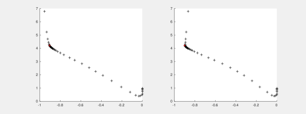
Figure 1: Pareto curves of our estimators. Left panel is the plot of of the estimated correlation $\hat{u}^{T}X^{T}Y\hat{v}$ versus the sum of $\|\hat{u}\|_{\ell_{1}}$ and $\|\hat{v}\|_{\ell_{1}}$, averaged over 100 simulations. The red dot corresponds to the ($u^{T}X^{T}Yv$, $\|u\|_{\ell_{1}}+\|v\|_{\ell_{1}}$). Right panel is the plot of the estimated correlation $\hat{u}^{T}\Sigma_{XY}\hat{v}$ versus the sum of $\|\hat{u}\|_{\ell_{1}}$ and $\|\hat{v}\|_{\ell_{1}}$, averaged over 100 simulations. The red dot corresponds to the ($u^{T}\Sigma_{XY}v$, $\|u\|_{\ell_{1}}+\|v\|_{\ell_{1}}$). Note that the red dot is on the pareto curve, which means that our algorithm achieve this optimal value with right choice of regularizers.

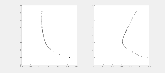
Figure 2: Pareto curves of Witten et al. [11]. Left panel is the plot of of the estimated correlation $\hat{u}^{T}X^{T}Y\hat{v}$ versus the sum of $\|\hat{u}\|_{\ell_{1}}$ and $\|\hat{v}\|_{\ell_{1}}$, averaged over 100 simulations. The red dot corresponds to the ($u^{T}X^{T}Yv$, $\|u\|_{\ell_{1}}+\|v\|_{\ell_{1}}$). Right panel is the plot of the estimated correlation $\hat{u}^{T}\Sigma_{XY}\hat{v}$ versus the sum of $\|\hat{u}\|_{\ell_{1}}$ and $\|\hat{v}\|_{\ell_{1}}$, averaged over 100 simulations. The red dot corresponds to the ($u^{T}\Sigma_{XY}v$, $\|u\|_{\ell_{1}}+\|v\|_{\ell_{1}}$). Note that the red dot is not on the pareto curve, which means that their algorithm could not achieve this optimal value with any choice of regularizers.

The left panel of Figure 1 is the plot of of the estimated correlation $\hat{u}^{T}X^{T}Y\hat{v}$ versus the sum of $\|\hat{u}\|_{\ell_{1}}$ and $\|\hat{v}\|_{\ell_{1}}$, averaged over 100 simulations. The right panel is the plot of estimated correlation $\hat{u}^{T}\Sigma_{XY}\hat{v}$ versus the sum of $\|\hat{u}\|_{\ell_{1}}$ and $\|\hat{v}\|_{\ell_{1}}$, averaged over 100 simulations. Note that we replace the sample covariance with the true covariance. From both panels, with the right choice of regularizers, our algorithm can achieve the optimal values. However, as shown in Figure 2, the solutions of Witten et al. [11] are very far from the true solution. The red dots are not on their solutions’ path, meaning that their results do not achieve the optimal value with any choices of regularizers. $\clubsuit$

2.2 Algorithmic details

2.2.1 Linearized alternating direction minimization method

We assume that the data matrix $X$ and $Y$ are centred. We now present how to solve the minimization problem Equation 4 in detail, and the algorithm works similarly for $v$.

With the data matrix $X$ and $Y$, the minimization Equation 4 becomes

$$\underset{u}{\text{minimize}}-u^{T}X^{T}Yv+\tau_{1}\|u\|_{1}+\mathbbm{1}\{u:\|Xu\|_{2}\leq 1\}.$$ (7)

Let $z=Xu$, we have

$$\underset{u}{\text{minimize}}\ \ \ \underbrace{-u^{T}X^{T}Yv+\tau_{1}\|u\|_{1}}_{f(u)}+\underbrace{\mathbbm{1}\{\|z\|_{2}\leq 1\}}_{g(z)}$$

subject to $$Xu=z$$ (8)

We can use linearized alternating direction method of multipliers [8] to solve this problem. The alternating direction method of multipliers is to solve the augmented Lagrangian by solving each variable and the dual variable one by one until convergence. The detailed derivation can be seen in Appendix and the complete algorithm can be seen in Algorithm 1.

2.2.2 TFOCS

The other approach to solve Equation 4 is to use TFOCS. We rewrite the Equation 4 as follows and use tfocs_SCD function to solve it.

Since $v$ is fixed, and let $c=v^{T}Y^{T}X$, minimizing the objective function of Equation 7

$$-cu+\tau_{1}\|u\|_{1}+\mathbbm{1}\{\|Xu\|_{2}\leq 1\}$$ (9)

is equivalent to minimizing

$$-cu/\tau_{1}+\|u\|_{1}+\mathbbm{1}\{\|Xu\|_{2}\leq 1\}$$

Instead of solving this objective function, we solve instead

$$\|u\|_{1}+\frac{1}{2}\mu\|u-(u_{old}+\frac{1}{\tau\mu}c)\|_{2}^{2}+\mathbbm{1}\{\|Xu\|_{2}\leq 1\}$$

Intuitively, we solve the Equation 9 without going too far from current approximation. This formulation can be solved using tfocs_SCD. [2].

Algorithm 1 Sparse CCA

1:function CCA($X,Y$)

2:     Initialize $u_{0}$ and $v_{0}$

3:     while not converged do

4:         Fix $v_{k}$

5:         while not converged do

$$u^{k+1} \leftarrow\mathbf{prox}_{\mu f}(u^{k}-\frac{\mu}{\lambda}X^{T}(Xu^{k}-z^{k}+\xi^{k}))$$

$$z^{k+1} \leftarrow\mathbf{prox}_{\lambda g}(Xu^{k+1}+\xi^{k})$$

$$\xi^{k+1} \leftarrow\xi^{k}+Xu^{k+1}-z^{k+1}$$

6:         end while

7:         Fix $u_{k}$,

8:         while not converged do

$$v^{k+1} \leftarrow\mathbf{prox}_{\mu f}(v^{k}-\frac{\mu}{\lambda}Y^{T}(Yv^{k}-z^{k}+\xi^{k}))$$

$$z^{k+1} \leftarrow\mathbf{prox}_{\lambda g}(Yv^{k+1}+\xi^{k})$$

$$\xi^{k+1} \leftarrow\xi^{k}+Yv^{k+1}-z^{k+1}$$

9:         end while

10:     end while

11:end function

2.3 The remaining canonical vectors

Given the first $r-1$ canonical vectors $U=\begin{pmatrix}u_{1}&\cdots&u_{r-1}\end{pmatrix}$ and $\begin{pmatrix}v_{1}&\cdots&v_{r-1}\end{pmatrix}$, we consider solving the $r$-th canonical vectors by

$$\underset{u,v}{\text{minimize}}\ \ \ -u^{T}X^{T}Yv+\tau_{1}|u|_{1}+\tau_{2}|v|_{1}+\mathbbm{1}\{u:\|Xu\|_{2}\leq 1\}+\mathbbm{1}\{v:\|Yv\|_{2}\leq 1\}$$

subject to $$U^{T}X^{T}Xu=0;V^{T}Y^{T}Yv=0.$$

This problem is biconvex, and we use the same approach of fixing one variable and solve for the other one. Fixing $v$, we get $\hat{u}$ by solving

$$\underset{u}{\text{minimize}}\ \ \ -u^{T}X^{T}Yv+\tau_{1}|u|_{1}+\mathbbm{1}\{z:\|z\|_{2}\leq 1\}$$

subject to $$Xu=z;U^{T}X^{T}Xz=0_{r-1},$$

and fixing $u$, we get $\hat{v}$ by solving

$$\underset{v}{\text{minimize}}\ \ \ -u^{T}X^{T}Yv+\tau_{1}|v|_{1}+\mathbbm{1}\{z:\|z\|_{2}\leq 1\}$$

subject to $$Yv=z;V^{T}Y^{T}Yz=0_{r-1}.$$

The constraint can be combined as

$$\begin{pmatrix}X\\ U^{T}X^{T}X\end{pmatrix}u-\begin{pmatrix}I\\ 0\end{pmatrix}z=0\quad\begin{pmatrix}Y\\ V^{T}T^{T}Y\end{pmatrix}v-\begin{pmatrix}I\\ 0\end{pmatrix}z=0$$

Let $\tilde{X}=\begin{pmatrix}X\\ U^{T}X^{T}X\end{pmatrix}$, fixing $v$, we can easily see that

$$-u^{T}X^{T}Yv=-u^{T}\tilde{X}^{T}Yv,$$

and fixing $u$,

$$-u^{T}X^{T}Yv=-u^{T}X^{T}\tilde{Y}v.$$

Therefore, we can use the linearized ADMM with the new matrix $\tilde{X}$ and $\tilde{Y}$ to get the $r$-th canonical vectors.

2.4 A bridge for the covariance matrix

As mentioned in section 2, [11] proposed to replace the covariance matrix with an identity matrix. Since their solution can be solved efficient, it is of interest to investigate the relation between our method and theirs. Therefore, we now write the covariance matrix as

$$\alpha_{x}X^{T}X+(1-\alpha_{x})\mathbf{I}_{p_{u},p_{u}}.$$

We can replace similarly for $Y$.

The constraint $\|Xu\|_{2}^{2}$ gives

$$u^{T}(\alpha_{x}X^{T}X+(1-\alpha_{x})\mathbf{I})u =\alpha_{x}\|Xu\|_{2}^{2}+(1-\alpha_{x})\|u\|_{2}^{2}=\|\begin{pmatrix}\alpha_{x}X\\ (1-\alpha)\mathbf{I}_{p_{u},p_{u}}\end{pmatrix}u\|_{2}^{2}.$$

This form can be solved using the methods we proposed by changing the linear operator with the matrix above. If interested to see how solutions change from Witten et al. [11] to our solution, one can use the above to see the path using different choices of $\alpha_{x},\alpha_{y}$.

2.5 Semidefinite Programming Approach

We now show that Equation 3 can be solved using a semi-definite programming approach. This idea is not new, but borrowed from the approach to solve sparse principle components [4] with some modifications. Let $h=\begin{pmatrix}u\\ v\end{pmatrix}$, the problem of

$$\begin{array}[]{ll}\mbox{minimize}&-u^{T}X^{T}Yv\\ \mbox{subject to}&u^{T}X^{T}Xu=1;v^{T}Y^{T}Yv=1\\ &|v|\leq t_{v};|u|\leq t_{u}\end{array}$$ (10)

can be written as

$$\begin{array}[]{ll}\mbox{minimize}&-\frac{1}{2}h^{T}\begin{pmatrix}0&X^{T}Y\\ Y^{T}X&0\end{pmatrix}h\\ \mbox{subject to}&h^{T}\begin{pmatrix}X^{T}X&0\\ 0&0\end{pmatrix}h=1;h^{T}\begin{pmatrix}0&0\\ 0&Y^{T}Y\end{pmatrix}h=1\\ &|h1_{v}|\leq t_{v};|h1_{u}|\leq t_{u}\end{array}$$ (11)

Now, we transfer the objective function using a trace operation:

$$-\frac{1}{2}h^{T}\begin{pmatrix}0&X^{T}Y\\ Y^{T}X&0\end{pmatrix}h=-\textbf{trace}(\begin{pmatrix}0&X^{T}Y\\ Y^{T}X&0\end{pmatrix}hh^{T})\$$

Let $H=hh^{T}$ and

$$Q=\begin{pmatrix}0&X^{T}Y\\ Y^{T}X&0\end{pmatrix};Q_{X}=\begin{pmatrix}X^{T}X&0\\ 0&0\end{pmatrix};Q_{Y}=\begin{pmatrix}0&0\\ 0&Y^{T}Y\end{pmatrix}$$

$$h^{T}\begin{pmatrix}X^{T}X&0\\ 0&0\end{pmatrix}h=\textbf{trace}(\begin{pmatrix}X^{T}X&0\\ 0&0\end{pmatrix}H)$$

$$\begin{array}[]{ll}\mbox{minimize}&-\textbf{trace}(QH)+\lambda\sum_{i,j}|H_{ij}|\\ \mbox{subject to}&H\in\mathbb{S}_{+}^{p_{u}+p_{v}}\\ &\textbf{trace}(Q_{X}H)=1;\textbf{trace}(Q_{y}H)=1\end{array}$$ (12)

Semi-definite programming problem can be very computational expansive, especially when $p$ is much greater than $n$ Therefore, we do not compute the sparse canonical vectors using this formulation. It would be a interesting direction to explore if there exists an efficient algorithm to solve this problem efficiently.

3 A Special Case

In this section, we consider a special case, where the covariance matrices of $x$ and $y$ is identity. Suppose that the matrices $\Sigma_{x}=\Sigma_{y}=I$, and thus the covariance matrix $\Sigma_{xy}=U\Lambda V^{T}$, where $U\in\mathbb{R}^{p\times k},V\in\mathbb{R}^{q\times k}$, and $\Lambda\in\mathbb{R}^{k\times k}$ is diagonal. In other words, $\Sigma_{xy}$ is rank $k$. We now show that our problem is similar to solving a sparse principle component analysis. Note that $U^{T}U=I_{k}$ and $V^{T}V=I_{k}$.

$$\begin{pmatrix}X\\ Y\end{pmatrix}\sim\mathsf{N}\big{(}\begin{pmatrix}0\\ 0\end{pmatrix}\begin{pmatrix}I&U\Lambda V^{T}\\ V\Lambda U^{T}&I\end{pmatrix}\big{)}$$

Theorem 2.

Estimation of $u$ and $v$ can be obtained using spectral decomposition and thus we can use software which solves sparse principle components to solve the problem above.

Proof    Let $\Sigma=A+I=\begin{pmatrix}0&U\Lambda V^{T}\\ V\Lambda U^{T}&0\end{pmatrix}+\begin{pmatrix}I&0\\ 0&I\end{pmatrix}$.

$$A=\begin{pmatrix}0&U\Lambda V^{T}\\ V\Lambda U^{T}&0\end{pmatrix}=\frac{1}{2}\begin{pmatrix}U\\ V\end{pmatrix}\Lambda\begin{pmatrix}U^{T}&V^{T}\end{pmatrix}-\frac{1}{2}\begin{pmatrix}U\\ -V\end{pmatrix}\Lambda\begin{pmatrix}U^{T}&-V^{T}\end{pmatrix}$$

Let $U_{i},V_{i}$ denote the $i$th columns of $U$ and $V$ respectively, and denote

$$W_{i}=\frac{1}{\sqrt{2}}\begin{pmatrix}U_{i}\\ V_{i}\end{pmatrix},\qquad W_{k+i}=\frac{1}{\sqrt{2}}\begin{pmatrix}U_{i}\\ -V_{i}\end{pmatrix}$$

for $i=1,\dots,k$. Note that $W_{i}^{T}W_{j}=\mathbb{I}(i=j)$, for $i,j=1,\dots,2k$. Let $\{W_{i}\}_{i=2k+1}^{p_{u}+p_{v}}$ be an orthonormal set of vectors orthogonal to $\{W_{i}\}_{i=1}^{2k}$. Then the matrix $\Sigma=A+I$ has the following spectral decomposition

$$\Sigma=\sum_{i=1}^{k}(1+\Lambda_{i,i})W_{i}W_{i}^{T}+\sum_{i=k+1}^{2k}(1-\Lambda_{i-k,i-k})W_{i}W_{i}^{T}+\sum_{i=2k+1}^{p_{u}+p_{v}}W_{i}W_{i}$$

Therefore, $\Sigma$ can be thought as a spiked covariance matrix, where the signal to noise ratio (SNR) can be interpreted as $1+\min_{i}\Lambda_{i,i}$. We know that in the high dimensional regime, if

$$\text{SNR}\geq\sqrt{\frac{p}{n}}$$

we can recover $u$ and $v$ even if $u$ and $v$ are not sparse. However, if

$$\text{SNR}<\sqrt{\frac{p}{n}},$$

we need to enforce the sparsity in $u$ and $v$, see Baik et al. [1] and Paul [9] for details. ∎

We can see from Theorem 2 that if the covariance matrices of $x$ and $y$ are identity, or act more or less like identity matrices, solving canonical vectors can be roughly viewed as solving sparse principle components. Therefore, in this case, estimating canonical vectors is roughly as hard as solving sparse eigenvectors.

4 Simulated Data

In this section, we carefully analyze different cases of covariance structure of $x$ and $y$ and compare the performance of our methods with other methods. We first explain how we generate the data.

Let $X\in\mathbb{R}^{n\times p}$ and $Y\in\mathbb{R}^{n\times q}$ be the data generated from the model

$$\begin{pmatrix}x\\ y\end{pmatrix}\sim\mathsf{N}\big{(}\begin{pmatrix}0\\ 0\end{pmatrix},\begin{pmatrix}\Sigma_{x}&\Sigma_{xy}\\ \Sigma_{yx}&\Sigma_{y}\end{pmatrix}\big{)},$$

where $\Sigma_{xy}=\rho\Sigma_{x}uv^{T}\Sigma_{y}$, where $u$ and $v$ are the true canonical vectors, and $\rho$ is the true canonical correlation. We would like to estimate $u$ and $v$ from the data matrices $X$ and $Y$. We compare our methods with other methods available on different choices of triplets: $(n,p,q)$, where $n$ is the number of samples, $p$ is the number of features in $X$, and $q$ is the number of features in $Y$. In order to measure the discrepancy of estimated $\hat{u}$, $\hat{v}$ with the true $u$ and $v$, we use the sin of the angle between $\hat{u}$ and $u$, $\hat{v}$ and $v$ Johnstone and Lu

$$\textbf{Loss}(\hat{v},v) =\min(\|\hat{v}-v\|_{2}^{2},\|\hat{v}+v\|_{2}^{2}$$ (13)

$$=2(1-|\left\langle\hat{v},v\right\rangle|),$$ (14)

where $\|\hat{v}\|_{2}=\|v\|_{2}=1$.

4.1 Identity-like covariance models

In sparse canonical correlation analysis literature, structured covariance of $x$ and $y$ are highly investigated. For examples, covariance of $x$ may be identity covariance, toeplitz, or have sparse inverse covariance. From the plot of the covariances matrix in Figure 3 and Figure 4, we can see toeplitz and sparse inverse covariance act more or less like identity matrices. Since the covariance of $x$ and $y$ act more or less like identity matrices, as discussed in previous section, solving $u$ and $v$ is roughly as hard as solving sparse eigenvectors. In other words, the covariance of $x$ and $y$ do not change the signal in $u$ and $v$ much and as a result, the signal in $\Sigma_{x}y$ is very sparse. In this case, an initial guess is very important. We propose the following procedure:

1. Denoise the matrix $X^{T}Y$ by solft-thresholding the matrix elementwise, call the resulting matrix as $S_{xy}$.

2. We obtain the initial guess as follows:

   1. Take singular value decomposition of $S_{xy}$, denoted as $\hat{U}$ and $\hat{V}$.

   2. Normalize the each column $u_{i}$, $v_{i}$ in $\hat{U}$ and $\hat{V}$ by $u_{i}\leftarrow\frac{u_{i}}{\sqrt{u_{i}^{T}(X^{T}X)u_{i}}}$ and $v_{i}\leftarrow\frac{v_{i}}{\sqrt{v_{i}^{T}Y^{T}Yv_{i}}}$. Denote the resulting $\hat{U}$ and $\hat{V}$ as $\tilde{U}$ and $\tilde{V}$.

   3. Calculate $\tilde{D}=\tilde{U}^{T}X^{T}Y\tilde{V}$ Choose the index $k$ where the maximum diagonal element of $\tilde{D}$ is obtained, i.e., $\mathop{\rm diag}(D)_{k}=\max\{\mathop{\rm diag}(D)\}$

3. Use the initial guess to start the alternating minimization algorithm.

We consider three types of covariance matrices in this category: toeplitz, identity, and sparse inverse matrices.

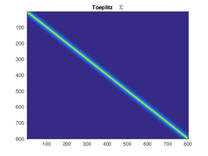
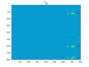
Figure 3: Toeplitz matrices with $\sigma_{ij}=0.9^{|i-j|}$: we can see that even though it is not exactly identity matrix, the general structure does look like identity matrix.

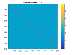
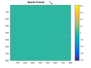
Figure 4: Sparse inverse matrix.

1. $\Sigma=I_{p}$.

2. $\Sigma=(\sigma_{ij})$, where $\sigma_{ij}=0.9^{|i-j|}$ for all $i,j\in p,q$. Here $\Sigma$ are Toeplitz matrices. See the plot of the toeplitz matrx and its corresponding $\Sigma_{xy}=\Sigma_{x}\rho uv^{T}\Sigma_{y}$. We can see that though it is not identity matrix, it behaves more or less like an identity matrix. Note that the smaller the toeplitz constant is, the more it looks like an identity matrix.

3. $\Sigma=(\frac{\sigma^{0}_{ij}}{\sqrt{\sigma^{0}_{ii}}\sigma^{0}_{jj}})$. Let $\Sigma^{0}=(\sigma_{ij}^{0})=\Omega^{-1}$ where $\Omega=(\omega_{ij})$ with

   $$\omega_{ij}=\mathbbm{1}_{\{i=j\}}+0.5\times\mathbbm{1}_{\{|i-j|=1\}}+0.4\times\mathbbm{1}_{\{|i-j|=2\}},i,j\in[p]$$

   In this case, $\Sigma_{x}$ and $\Sigma_{y}$ have sparse inverse matrices.

In each example, we simulate 100 data sets, i.e., 100 $X$, and 100 $Y$ in order to average our performance. We set the number of non-zeros in the $u$ and $v$ to be 5, the index of nonzeros are randomly chosen. We will vary the number of nonzeros in the next comparison. For each simulation, we have a sequence of regularizer $\tau_{u}$ and $\tau_{v}$ to choose from. For simplicity, we chose the best $\tau_{u}$ and $\tau_{v}$ such that estimated $\hat{u}$ and $\hat{v}$ minimize the Loss defined above in every methods.

We present our result in the Table 2, Table 3 and Table 4. There are some notations presented in the table and we now explain them here. $\hat{\rho}$ is the estimated canonical correlation between data $X$ and $Y$. $e_{u}=\textbf{Loss}(\hat{u},u)$ and $e_{v}=\textbf{Loss}(\hat{u},u)$. We compare our result with the methods proposed by Witten et al. [11], and Gao et al. [5]. Since we are not able to run the code from Tan et al. [10] very efficiently, we will compare our method with their approach in the next subsection. In order to compare them in the same unit, we calculate the estimates of each method and then normalize them by $X\hat{u}$, and $Y\hat{v}$ respectively. We then normalize estimates such that they all have norm 1. We report the estimated correlation, loss of $u$ and loss of $v$ as a format of $(\rho,e_{u},e_{v})$ for each method in all tables. From Table 2, Table 3, and Table 4, we can see that SCCA method proposed by Gao et al. [5] performs similarly with ours. However, their two step procedure is computationally expensive compared to ours and hard to choose regularizers. Estimates by Witten et al. [11] fails to provide accurate approximations because of the low samples size we considered.

$(n,p,q)$	Our method	SCCA	PMA
(400, 800,800)	(0.90,0.056,0.062)	(0.90,0.060,0.066)	(0.71,1.17, 1.17)
(500, 600, 600)	(0.90,0.05,0.056)	(0.90, 0.053, 0.057)	(0.71,0.85,0.85)
(700, 1200,1200)	(0.90,0.045, 0.043)	(0.90,0.045, 0.043)	(0.71, 1.09,1.09)

Table 2: Error comparison for identity matrices: we use a format of $(\hat{\rho},\textbf{Loss}(\hat{u}),\textbf{Loss}(\hat{v})$ to represent each method’s result.

$(n,p,q)$	Our method	SCCA	PMA
(400, 800, 800)	(0.91, 0.173 ,0.218)	(0.91, 0.213, 0.296)	(0.52,1.038,1.067)
(500, 600, 600)	(0.90, 0.136, 0.098)	(0.90, 0.145, 0.109)	(0.55, 1.11, 0.94)
(700, 1200, 1200)	(0.90, 0.109, 0.086)	(0.90, 0.110, 0.088)	(0.60, 1.098,0.89)

Table 3: Error comparison for toeplitz matrices: we use a format of $(\hat{\rho},\textbf{Loss}(\hat{u}),\textbf{Loss}(\hat{v})$ to represent each method’s result.

$(n,p,q)$	Our method	SCCA	PMA
(400, 800, 800)	(0.92,0.092,0.149)	(0.92,0.129, 0.190)	(0.61, 0.93, 1.0)
(500, 600, 600)	(0.90, 0.068, 0.059)	(0.90, 0.069, 0.0623)	(0.7215, 0.67 0.45)
(700, 1200, 1200)	(0.90, 0.050 ,0.044)	(0.90, 0.051, 0.047)	(0.70, 0.76, 0.58)

Table 4: Error comparison for sparse inverse matrices: we use a format of $(\hat{\rho},\textbf{Loss}(\hat{u}),\textbf{Loss}(\hat{v})$ to represent each method’s result.

4.2 Spiked covariance models

In this subsection, we consider covariance matrices of $x\in\mathbb{R}^{p}$ and $y\in\mathbb{R}^{q}$ are spiked, i.e.,

$$\mathop{\rm Cov}(x)=\sum_{i=1}^{k_{x}}\lambda_{i}w_{i}w_{i}^{T}+I_{p},$$

$$\mathop{\rm Cov}(y)=\sum_{i=1}^{k_{y}}\lambda_{i}w_{i}w_{i}^{T}+I_{q}.$$

In Example subsection 4.2 we will see that even we have the more observations with the number of features, the traditional singular value decomposition can return bad results.

Example 2:  We generate the $\Sigma_{x}$ and $\Sigma_{y}$ as follows:

$$\Sigma_{x} =\sum_{i=1}^{k}\lambda_{x,i}w_{x,i}w_{x,i}^{T}+I$$

$$\Sigma_{y} =\sum_{i=1}^{k}\lambda_{y,i}w_{y,i}w_{y,i}^{T}+I$$

where $w_{x,1},\cdots w_{x,k}$, $\mathbb{R}^{p}$, $w_{y,1},\cdots w_{y,k}$ are independent orthonormal vectors in $\mathbb{R}^{p}$, $\mathbb{R}^{q}$ respsectively, and $\lambda_{x,i}=\lambda_{y,i}=250$ and $k=20$. The covariance $\Sigma_{xy}$ is generated as

$$\Sigma_{xy}=\Sigma_{x}\rho uv^{T}\Sigma_{y},$$

where $u$ and $v$ are the true canonical vectors and have 10 nonzero elements with indices randomly chosen. We generate the data matrices $X\in\mathbb{R}^{n\times p}$ and $Y^{n\times q}$ from the distribution

$$\begin{pmatrix}x\\ y\end{pmatrix}\sim\mathsf{N}(\begin{pmatrix}0\\ 0\end{pmatrix},\begin{pmatrix}\Sigma_{x}&\Sigma_{xy}\\ \Sigma_{xy}^{T}&\Sigma_{y}\end{pmatrix}.$$

Therefore, when $n=1000,p=800,q=800$, we should be able to estimate $u$ and $v$ using the singular value decomposition of the matrix

$$\hat{\Sigma}_{x}^{-1/2}\hat{\hat{\Sigma}}_{xy}\hat{\Sigma}_{y}^{-1/2}=(X^{T}X)^{-1/2}(X^{T}Y)(Y^{T}Y)^{-1/2}.$$

However, the estimated $\hat{u}$ and $\hat{v}$ can be seen in Figure 5. The results are wrong and not sparse. This is an indication that we need more samples to estimate the canonical vectors. As we increase the sample size to $n=3000$, estimates of $u$ and $v$ are more accurate but not very sparse, as seen in Figure 6. For our method, we use $n=400$, the estimated $\hat{u}$ and $\hat{v}$ of our methods can be seen in Figure 7. Our method returns sparse and better estimates for $u$ and $v$.

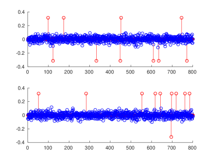
Figure 5: Plot of Estimated $\hat{u}$, $\hat{v}$ from singular value decomposition (blue) and true $u$, $v$ (red), The number of observations $n=1000$, with $p=800,q=800$. Estimated $u$ and $v$ using singular value decomposition of the transformed estimated covariance matrix are not good estimated of the true $u$ and $v$. The results are wrong and not sparse. This is an indication that we need more samples to estimate the canonical vectors.

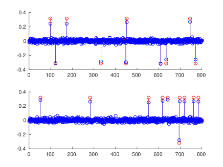
Figure 6: Plot of Estimated $u$, $v$ from singular value decomposition (blue) and true $u$, $v$ (red), The number of observations $n=1000$, with $p=800,q=800$. Estimated $u$ and $v$ using singular value decomposition of the transformed estimated covariance matrix are not good estimated of the true $u$ and $v$. The results are wrong and not sparse. This is an indication that we need more samples to estimate the canonical vectors.

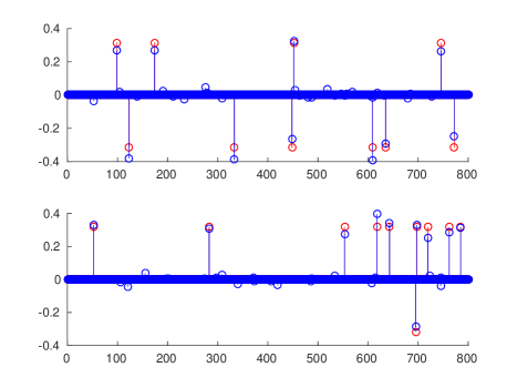
Figure 7: Plot of Estimated $u$, $v$ from our method (blue) and true $u$, $v$ (red), The number of observations is $n=400$, with $p=800,q=800$. Note that we use less samples than the results of the Figure 5. We can successfully recover the correct support using our method.

$\clubsuit$

4.3 A detailed Comparison

To further illustrate the accuracy of our methods, we compare our methods with the methods proposed by Tan et al. [10] using the plot of scaled sample size versus estimation error. Here we choose the same set up with their setup since their method performed the best in comparison with PMA. The data was simulated as follows:

$$\rho=0.9,u_{j}=\frac{1}{\sqrt{5}},v_{j}=\frac{1}{\sqrt{5}}\text{ for }j=1,6,11,16,21.$$

And $\Sigma_{x}$ and $\Sigma_{y}$ are block diagonal matrix with five blocks, each of dimension $d/5\times d/5$, where the $(j,j^{\prime})$ th element of each block takes value $0.7^{|j-j^{\prime}|}$. The result is done for $p_{u}=300$, $p_{v}=300$ and average over 100 simulations.

Though the set up of our simulation is the same with Tan et al. [10], we would like to investigate when the rescaled sample size is small, i.e., when the number of samples is small. As shown in Figure 8, our method outperforms their method.

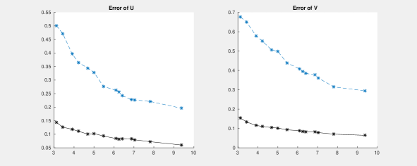
Figure 8: A comparison between performance of our method and method proposed by Tan et al. [10]. The left panel is the $\textbf{Loss}(\hat{u})$ versus rescaled sample size $n/s\log(d)$, and the right panel is the $\textbf{Loss}(\hat{v})$ versus rescaled sample size $n/s\log d$. Blue line is the result of Tan et al. [10] and the black line is the result of our method.

5 Discussion and future work

We proposed a sparse canonical correlation framework and show how to solve it efficiently using ADMM and TFOCS. We presented different simulation scenarios and showed our estimates are more sparse and accurate. Though our formulation is non-convex, global solutions are often obtained, as seen among simulated examples. We are currently working on some applications on real data sets.

6 Appendix

Detailed derivations for linearized ADMM

The augmented Lagrangian form of 8 is

$$L(u,z,\xi)=-u^{T}X^{T}Yv+\tau_{1}\|u\|_{1}+\mathbbm{1}\{\|z\|_{2}\leq 1\}+\phi^{T}(Xu-z)+\frac{\rho}{2}\|Xu-z\|_{2}^{2}.$$

Thus, the updates of variables are solved through

$$u^{k+1} =\text{argmin}_{u}\{-u^{T}X^{T}Yv+\tau_{1}\|u\|_{1}+{\phi^{k}}^{T}(Xu-z^{k})+\frac{\rho}{2}\|Xu-z^{k}\|_{2}^{2}\}$$

$$z^{k+1} =\text{argmin}_{z}\{\mathbbm{1}\{\|z\|_{2}\leq 1\}+\phi^{T}(Xu^{k+1}-z)+\frac{\rho}{2}\|Xu^{k+1}-z\|_{2}^{2}\}$$

$$\phi^{k+1} =\phi^{k}+\rho(Xu^{k+1}-z^{k+1})$$

Now, we let $\xi^{k}=\frac{\phi^{k}}{\rho}$ and add some constants, and we get

$$u^{k+1} =\text{argmin}_{u}\{-u^{T}X^{T}Yv+\tau_{1}\|u\|_{1}+\rho{\xi^{k}}^{T}(Xu-z^{k})+\frac{\rho}{2}\|Xu-z^{k}\|_{2}^{2}+\frac{\rho}{2}\|\xi\|_{2}^{2}\}$$

$$z^{k+1} =\text{argmin}_{z}\{\mathbbm{1}\{\|z\|_{2}\leq 1\}+\rho\xi^{T}(Xu^{k+1}-z)+\frac{\rho}{2}\|Xu^{k+1}-z\|_{2}^{2}+\frac{\rho}{2}\|\xi\|_{2}^{2}\}$$

$$\xi^{k+1} =\xi^{k}+(Xu^{k+1}-z^{k+1}).$$

Therefore, we have

$$u \leftarrow\text{argmin}_{u}\{-u^{T}X^{T}Yv+\tau_{1}\|u\|_{1}+\frac{\rho}{2}\|Xu-z+\xi\|_{2}^{2}\}$$

$$z \leftarrow\text{argmin}_{z}\{\mathbbm{1}\{\|z\|_{2}\leq 1\}+\frac{\rho}{2}\|Xu-z+\xi\|_{2}^{2}\}$$

$$\xi \leftarrow\xi+(Xu-z).$$

The linearized ADMM replace the quadratic term by a linear term in order to speed up:

$$u \leftarrow\text{argmin}_{u}\{-u^{T}X^{T}Yv+\tau_{1}\|u\|_{1}+\rho(X^{T}Xu^{k}-X^{T}z^{k})^{T}u+\frac{\mu}{2}\|u-u^{k}\|_{2}^{2}\}$$

$$z \leftarrow\text{argmin}_{z}\{\mathbbm{1}\{\|z\|_{2}\leq 1\}+\frac{\rho}{2}\|z-Xu^{k+1}+\xi^{k}\|_{2}^{2}\}$$

$$\xi \leftarrow\xi+(Xu^{k+1}-z^{k+1}).$$

Let $\rho=1/\lambda$, and $\mu=\frac{1}{\mu}$, we get

$$u \leftarrow\text{argmin}_{u}\{-u^{T}X^{T}Yv+\tau_{1}\|u\|_{1}+\frac{1}{\lambda}(X^{T}Xu^{k}-X^{T}z^{k})^{T}u+\frac{1}{2\mu}\|u-u^{k}\|_{2}^{2}\}$$

$$z \leftarrow\text{argmin}_{z}\{\mathbbm{1}\{\|z\|_{2}\leq 1\}+\frac{\rho}{2}\|z-Xu^{k+1}+\xi^{k}\|_{2}^{2}\}$$

$$\xi \leftarrow\xi+(Xu^{k+1}-z^{k+1}).$$

For the first minimization problem, after some simple algebra, we can get:

$$u^{k+1} =\text{argmin}_{u}\{-u^{T}X^{T}Yv+\tau_{1}\|u\|_{1}+\frac{1}{2\mu}\|u-(u^{k}-\frac{\mu}{\lambda}(X^{T}(Xu^{k}-z^{k}+\xi^{k}))\|_{2}^{2}\}$$

Therefore, our detailed updates are:

$$u^{k+1} \leftarrow\mathbf{prox}_{\mu f}(u^{k}-\frac{\mu}{\lambda}X^{T}(Xu^{k}-z^{k}+\xi^{k}))$$

$$z^{k+1} \leftarrow\mathbf{prox}_{\lambda g}(Xu^{k+1}+\xi^{k})$$

$$\xi^{k+1} \leftarrow\xi^{k}+Xu^{k+1}-z^{k+1}.$$

The analytic proximal mapping of $f$ and $g$ can be easily derived: $f(x)$ involves soft threshold and $g(x)$ is projection to the convex set (a norm ball):

$$\mathbf{prox}_{\mu f}(x)=\begin{cases}x+\mu c-\mu\tau&\text{ if }x+\mu c>\mu\tau\\ x+\mu c+\mu\tau&\text{ if }x+\mu c<-\mu\tau\\ 0&\text{ else }\end{cases}$$

$$\mathbf{prox}_{\lambda g}(x)=\begin{cases}x&\text{ if }\|x\|_{2}\leq 1\\ \frac{x}{\|x\|_{2}}&\text{ else}\end{cases}$$ (15)

where $c=X^{T}Yv$ (the gradient of the objective function with respect to one canonical vector while fixing the other canonical vector).

References

• Baik et al. [2005] Jinho Baik, Gérard Ben Arous, Sandrine Péché, et al. Phase transition of the largest eigenvalue for nonnull complex sample covariance matrices. The Annals of Probability, 33(5):1643–1697, 2005.
• Becker et al. [2011] Stephen R. Becker, Emmanuel J. Candès, and Michael C. Grant. Templates for convex cone problems with applications to sparse signal recovery. Mathematical Programming Computation, 3(3):165, 2011. ISSN 1867-2957. doi: 10.1007/s12532-011-0029-5. URL http://dx.doi.org/10.1007/s12532-011-0029-5.
• Chen et al. [2013] M. Chen, C. Gao, Z. Ren, and H. H. Zhou. Sparse CCA via Precision Adjusted Iterative Thresholding. ArXiv e-prints, November 2013.
• d’Aspremont et al. [2007] Alexandre d’Aspremont, Laurent El Ghaoui, Michael I. Jordan, and Gert R. G. Lanckriet. A direct formulation for sparse pca using semidefinite programming. SIAM Review, 49(3):434–448, 2007. doi: 10.1137/050645506.
• Gao et al. [2014] C. Gao, Z. Ma, and H. H. Zhou. Sparse CCA: Adaptive Estimation and Computational Barriers. ArXiv e-prints, September 2014.
• Hotelling [1936] HAROLD Hotelling. Relations between two sets of variates. Biometrika, 28(3-4):321–377, 1936. doi: 10.1093/biomet/28.3-4.321. URL http://biomet.oxfordjournals.org/content/28/3-4/321.short.
• Johnstone and Lu [2009] Iain M. Johnstone and Arthur Yu Lu. On consistency and sparsity for principal components analysis in high dimensions. Journal of the American Statistical Association, 104(486):682–693, 2009. doi: 10.1198/jasa.2009.0121. URL http://dx.doi.org/10.1198/jasa.2009.0121. PMID: 20617121.
• Parikh and Boyd [2014] Neal Parikh and Stephen Boyd. Proximal algorithms. Found. Trends Optim., 1(3):127–239, January 2014. ISSN 2167-3888. doi: 10.1561/2400000003. URL http://dx.doi.org/10.1561/2400000003.
• Paul [2007] Debashis Paul. Asymptotics of sample eigenstructure for a large dimensional spiked covariance model. Statistica Sinica, pages 1617–1642, 2007.
• Tan et al. [2016] K. M. Tan, Z. Wang, H. Liu, and T. Zhang. Sparse Generalized Eigenvalue Problem: Optimal Statistical Rates via Truncated Rayleigh Flow. ArXiv e-prints, April 2016.
• Witten et al. [2009] Daniela M. Witten, Robert Tibshirani, and Trevor Hastie. A penalized matrix decomposition, with applications to sparse principal components and canonical correlation analysis. Biostatistics, 10(3):515–534, 2009. doi: 10.1093/biostatistics/kxp008. URL http://biostatistics.oxfordjournals.org/content/10/3/515.abstract.