Scale anomaly of a Lifshitz scalar: a universal quantum phase transition to discrete scale invariance

Abstract

We demonstrate the existence of a universal transition from a continuous scale invariant phase to a discrete scale invariant phase for a class of one-dimensional quantum systems with anisotropic scaling symmetry between space and time. These systems describe a Lifshitz scalar interacting with a background potential. The transition occurs at a critical coupling $\lambda_{c}$ corresponding to a strongly attractive potential.

Some of the most intriguing phenomena resulting from quantum physics are the violation of classical symmetries, collectively referred to as anomalies Adler (1969); Bell and Jackiw (1969); Esteve (1986); Holstein (1993). One class of anomalies describes the breaking of continuous scale symmetry at the quantum level. A remarkable example of these “scale anomalies” occurs in the case of a non-relativistic particle in the presence of an attractive, inverse square potential Case (1950); de Alfaro et al. (1976); Landau (1991); Camblong et al. (2000); Aña nos et al. (2003); Hammer and Swingle (2006); Braaten and Phillips (2004); Kaplan et al. (2009), which describes the Efimov effect Efimov (1970, 1971); Braaten and Hammer (2006) and plays a role in various other systems Lévy-Leblond (1967); Kolomeisky and Straley (1992); Gupta and Rajeev (1993); Camblong et al. (2001); Nisoli and Bishop (2014); Govindarajan et al. (2000); Camblong and Ordonez (2003); Bellucci et al. (2003). Classically scale invariant Jackiw (1995), any system described by the Hamiltonian, $\hat{H}_{S}=p^{2}/2m-\lambda/r^{2}$, exhibits an abrupt transition in the spectrum at $2m\lambda_{c}=(d-2)^{2}/4$ where $d$ is the space dimension. For $\lambda<\lambda_{c}$, the spectrum contains no bound states close to $E=0$, however, as $\lambda$ goes above $\lambda_{c}$, an infinite series of bound states appears. Moreover, in this “over-critical” regime, the states arrange themselves in an unanticipated geometric series $E_{n}\propto\exp{(-2\pi n/\sqrt{\lambda-\lambda_{c}})}$, $n\in\mathbb{Z}$, accumulating at $E=0$. The existence and geometric structure of such levels do not rely on the details of the potential close to its source and is a signature of residual discrete scale invariance since $\{E_{n}\}\rightarrow\{\exp{(-2\pi/\sqrt{\lambda-\lambda_{c}}))}E_{n}\}=\{E_{n}\}$. Thus, $H_{S}$ exhibits a quantum phase transition at $\lambda_{c}$ between a continuous scale invariant (CSI) phase and a discrete scale invariant phase (DSI). This transition has been associated with Berezinskii-Kosterlitz-Thouless (BKT) transitions Kolomeisky and Straley (1992); Kaplan et al. (2009); Jensen et al. (2010); Jensen (2010, 2011); Derrida and Retaux (2014); Gies and Torgrimsson (2016).

Another system - the charged and massless Dirac fermion in an attractive Coulomb potential $\hat{H}_{D}=\gamma^{0}\gamma^{j}p_{j}-\lambda/r$ Ovdat et al. (2017) - also belongs to the same universal class of systems with these abrupt transitions. The similarity between the spectra and transition of these Dirac and Schrödinger Hamiltonians motivates the study of whether a transition of this sort is possible for a generic scale invariant system. Specifically, these different Hamiltonians share a similar property - the power law form of the corresponding potential matches the order of the kinetic term. In this paper, we examine whether this property is a sufficient ingredient by considering a generalised class of one dimensional Hamiltonians

$$\hat{H}_{N}=(p^{2})^{N}-\frac{\lambda_{N}}{x^{2N}}\;,$$ (1)

where $N$ is an integer and $\lambda_{N}$ a real coupling, and study if they exhibit a transition of the same universality class as $\hat{H}_{S}=\hat{H}_{1},\hat{H}_{D}$.

Hamiltonian (1) describes a system with non-quadratic anisotropic scaling between space and time for $N>1$. This “Lifshitz scaling symmetry” Alexandre (2011), manifest in (1), can be seen for example at the finite temperature multicritical points of certain materials Hornreich et al. (1975); Grinstein (1981) or in strongly correlated electron systems Fradkin et al. (2004); Vishwanath et al. (2004); Ardonne et al. (2004). It may also have applications in particle physics Alexandre (2011), cosmology Mukohyama (2010) and quantum gravity Reuter (1998); Kachru et al. (2008); Horava (2009a, b); Gies et al. (2016). The non-interacting mode ($\lambda_{N}=0$) can also appear very generically, for example in non-relativistic systems with spontaneous symmetry breaking Brauner (2010).

Generalising (1) to higher dimensional flat or curved spacetimes also introduces intermediate scale invariant terms which are products of radial derivatives and powers of the inverse radius. For $d>1$ the potential in (1) can be generated by considering a Lifshitz scale invariant system with charge and turning on a background gauge field Horava (2011); Das and Murthy (2010); Alexandre (2011); Farias et al. (2012) consisting of the appropriate multipole moment. The procedures we use throughout this paper are readily extended to these situations and the simple model (1) is sufficient to capture the desired features.

$N$	$1$		$2$		$3$
$\lambda$	$-\frac{3}{4}<\lambda_{1}$	$\lambda_{1}<-\frac{3}{4}$	$\frac{105}{16}<\lambda_{2}$	$-45<\lambda_{2}<\frac{105}{16}$	$693\lesssim\lambda_{3}$	$-162\lesssim\lambda_{3}\lesssim 693$
extension	$U(1)$	self-adjoint	$U(1)$	$U(2)$	$U(1)$	$U(3)$

Table 1: The regimes of self-adjoint extension parameter with $N=1,2,3$ for some values of $\lambda_{N}$. The bounds for $N=1,2$ are exact while those for $N=3$ are approximate and determined by numerically solving the indicial equation (2). A table showing $\lambda_{N}$, for $N=1,2,3$, to larger negative values can be found in the supplementary material.

Our main results are summarized as follows. In accordance with the $N=1$ case, there is a quantum phase transition at $\lambda_{N,c}\equiv(2N-1)!!^{2}/2^{2N}$ for all $N>1$ from a CSI phase to a DSI phase in the low energy regime $|E|^{1/2N}x_{0}\ll 1$, where $x_{0}>0$ is a short distance cutoff. The CSI phase contains no bound states and the DSI phase is characterized by an infinite set of bound states forming a geometric series as given by equation (11). The transition and $\lambda_{N,c}$ value are independent of the short distance physics characterised by the boundary condition at $x=x_{0}$. For $\left(\lambda_{N}-\lambda_{N,c}\right)\rightarrow 0^{+}$, the analytic behaviour of the spectrum is characteristic of the BKT scaling in analogy with $N=1$ Kolomeisky and Straley (1992); Kaplan et al. (2009) and as shown by equation (17). We analyse the $x_{0}=0$ case, obtain its self adjoint extensions and spectrum and obtain similar results.

I The model

Corresponding to (1) is the action of a complex scalar field in $(1+1)$-dimensions:

$$\int dt\int_{x=x_{0}}^{\infty}dx\;\frac{i}{2}\left(\Psi^{*}\partial_{t}\Psi-\mathrm{c.c.}\right)-\left|\partial_{x}^{N}\Psi\right|^{2}+\frac{\lambda_{N}}{x^{2N}}\left|\Psi\right|^{2}\;,$$

where $\mathrm{c.c.}$ indicates the complex conjugate. This field theory has manifest Lifshitz scaling symmetry, $(t,x)\mapsto(\Lambda^{2N}t,\Lambda x)$ when $x_{0}\rightarrow 0$. The scaling exponent of $\Lambda^{2}$ is called the “dynamical exponent” and has value $N$ in this case. The action represents a Lifshitz scalar with a single time derivative and can be recovered as the low energy with respect to mass limit of a charged, massive Lifshitz scalar which is quadratic in time derivatives Pal and Grinstein (2016). The eigenstates of Hamiltonian (1) are given by stationary solutions of the subsequent equations of motion .

Consider the case $x_{0}<x<\infty$ with $x_{0}=0$. The classical scaling symmetry of (1) implies that if there is one negative energy bound state then there is an unbounded continuum. Thus, the Hamiltonian is non-self-adjoint Bonneau et al. (2001); Ibort et al. (2015). The origin of this phenomenon, already known from the $N=1$ case, is the strong singularity of the potential at $x=0$. To remedy this problem, the operator can be made self-adjoint by applying boundary conditions on the elements of the Hilbert space through the procedure of self-adjoint extension Gitman et al. (2009). Alternatively, a suitable cutoff regularisation at $x_{0}>0$ can be chosen to ensure self-adjointness as well as bound the spectrum from below by an intrinsic scale Camblong et al. (2000) leaving some approximate DSI at low energies.

For $N=1$ in (1), the continuous scaling invariance of $\hat{H}_{1}$ is broken anomalously as a result of restoring self-adjointness. In particular, for $\lambda_{1}>1/4$, one obtains an energy spectrum given by $E_{1}=-E_{0}\exp\left(-(2\pi n)/\sqrt{\lambda_{1}-\lambda_{c}}\right)$ for $n\in\mathbbm{Z}$. The energies are related by a discrete family of scalings which manifest a leftover DSI in the system.

In what follows, we shall demonstrate that in the case of large positive $\lambda_{N}$ (attractive potential) one finds, for all $N$, a regime with a geometric tower of states using the method of self-adjoint extension. Subsequently, we bound the resulting spectrum from below, while maintaining DSI at low energies, by keeping $x_{0}>0$ and applying generic (self-adjoint) boundary conditions at a cut-off point. We obtain that a transition from CSI to DSI is a generic feature in the landscape of these Hamiltonians (1), independent of the choice of boundary condition and in a complete analogy with the $N=1$ case Case (1950); de Alfaro et al. (1976); Landau (1991); Camblong et al. (2000); Aña nos et al. (2003); Hammer and Swingle (2006); Braaten and Phillips (2004); Kaplan et al. (2009). By analytically solving the eigenvalue problem for all $N$, we obtain an expression for the critical $\lambda_{N}$ and for the resulting DSI spectrum in the over-critical regime.

II Self-adjoint extension

To determine whether the Hamiltonians (1) can be made self-adjoint one can apply von Neumann’s procedure Meetz (1964); Bonneau et al. (2001); Gitman et al. (2009, 2012a); Ibort et al. (2015). This consists of counting the normalisable solutions to the energy eigenvalue equation with unit imaginary energies of both signs. When there are $M$ linearly independent solutions of positive and negative sign respectively, there is a $U(M)$ parameter family of conditions at $x=0$ that can make the operator self-adjoint. If $M=0$, it is essentially self-adjoint and if the number of positive and negative solutions do not match then the operator cannot be made self-adjoint.

For every $N$, there are $N$ exponentially decaying solutions at infinity for $E=\pm i$. Normalisability then depends on their $x\rightarrow 0$ behaviour which requires a complete solution of the eigenfunctions. The energy eigenvalue equation from (1) has an analytic solution in terms of generalised hypergeometric functions Luke (1969) (see the supplementary material) for arbitrary complex energy and $\lambda_{N}$. Near $x=0$, the analytic solutions are characterised by the roots of the indicial equation,

$$\lambda_{N}=(-1)^{N}\Delta(\Delta-1)(\Delta-2)\ldots(\Delta-2N+1)\;,\qquad$$ (2)

which can be obtained by inserting $\Psi(x)=x^{\Delta}(1+\mathcal{O}(x^{2N}))$ into the eigenvalue equation and solving for $\Delta$. We label the $2N$ solutions of (2) as $\Delta_{i},i=1,\ldots,2N$ and order by ascending real part followed by ascending imaginary part. Since (2) is real and symmetric about $N-1/2$, all roots can be collected into pairs which sum to $2N-1$ (see fig. 1). In addition, because $N-1/2\geq-1/2$, there can be at most $N$ roots with $\mathrm{Re}(\Delta_{i})\leq-1/2$ . Thus, near $x=0$, a generic combination of the $N$ decaying solutions has the form:

$$\Psi(x) = \sum_{i=1}^{N}\left[\left(\epsilon x\right)^{\Delta_{i}}\phi_{i}+\ldots+\left(\epsilon x\right)^{\Delta_{i+N}}O_{i}+\ldots\right]\;,\qquad$$ (3)

where $E$ is the energy, $\epsilon\equiv|E|^{1/2N}$ and $\phi_{i},O_{i}$ are complex numbers . We have distinguished modes with the potential to be divergent as $x\rightarrow 0$ by the coefficients $\phi_{i}$. Taking ratios of $O_{i}$ and $\phi_{i}$ yields $N$ independent dimensionless scales.

To obtain the number of independent normalisable solutions $M$, we need to count the number $m$ of roots $\Delta_{i}$ with real parts less than $-1/2$ as $\lambda_{N}$ varies. When any root violates this bound we must take a linear combination of our $N$ decaying functions to remove it from the near origin expansion and as a result $M=N-m$. This is easily accomplished by examining the analytic solutions in an expansion about $x=0$.

Figure 1: A plot of the real part of the solution to the indicial equation (2) for $N=2$ against $\lambda_{2}$. The dotted, red vertical line indicates where $\lambda_{2}=9/16$ above which the first pair of complex roots appears. The lowermost horizontal red line indicates where one of the roots becomes non-normalisable at positive $\lambda_{2}$ (i.e. $\lambda_{2}=105/16$) while the uppermost indicates the symmetry line responsible for pairing roots i.e. $\Delta=3/2$.

Generically, for $\lambda_{N}$ small in magnitude, $m=0$, and there is an $U(N)$ self-adjoint extension . As $\lambda_{N}$ increases in absolute value and the real part of some roots go below $-1/2$ the dimension of the self-adjoint parameter decreases. Eventually $\hat{H}_{N}$ either becomes essentially self-adjoint (negative $\lambda_{N}$, repulsive potential) or has a $U(1)$ self-adjoint extension (positive $\lambda_{N}$, attractive potential). The different regimes are summarised for $N=1,2,3$ in table 1.

Now that we have determined when our operator can be made self-adjoint we would like to obtain its energy spectrum. To that purpose, we define the boundary form, $\left[\Psi,\Phi\right](x)$, by computing the difference $\hat{H}_{N}-\hat{H}^{\dagger}_{N}$ :

$$\langle\Phi|\hat{H}_{N}|\Psi\rangle - \langle\Phi|\hat{H}^{\dagger}_{N}|\Psi\rangle=\left[\Phi,\Psi\right](\infty)-\left[\Phi,\Psi\right](x_{0})\;,\qquad$$ (4)

$$\langle\Phi|\hat{H}_{N}|\Psi\rangle = \int_{x=x_{0}}^{\infty}dx\;\Phi^{*}(x)\hat{H}_{N}\Psi(x)\;,$$ (5)

where

$$\left[\Phi,\Psi\right](x)=\sum_{j=1}^{2N}(-1)^{N+j-1}d_{x}^{j-1}\Phi^{*}(x)d_{x}^{2N-j}\Psi(x)\;\qquad$$ (6)

and the boundary form is calculated by moving the derivatives in $\langle\Phi|\hat{H}_{N}|\Psi\rangle$ to obtain $\langle\Phi|\hat{H}_{N}^{\dagger}|\Psi\rangle$ (see supplementary material). Setting $\Phi=\Psi$ and using the time dependent Schrödinger equation it is straightforward to show that

$$\partial_{t}\rho=\partial_{x}\left[\Psi,\Psi\right]\;,\qquad\rho=|\Psi|^{2}\;,\qquad$$ (7)

so that the boundary form can be interpreted as the value of the probability current at $x=x_{0}$.

We are interested in evaluating (4) on the energy eigenfunctions and require it to vanish when taking $x_{0}\rightarrow 0$ as this fixes any remaining free parameters of a general solution. For $E<0$ there are $N$ exponentially decaying solutions at infinity. A general energy eigenfunction is a sum of these and thus the boundary form (4) evaluated at infinity is zero. For $\hat{H}_{N}$ to be self-adjoint it is necessary to impose the same boundary conditions on the wavefunctions and their adjoints while ensuring that (6) vanishes.

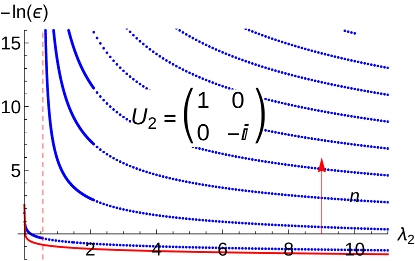
Figure 2: A plot of the logarithm of $\epsilon$ against $\lambda_{2}$ for a cut-off position $x_{0}=e^{-1}$ and boundary condition displayed. For $\lambda_{2}<\lambda_{2,c}=9/16$ there are no bound states satisfying $\epsilon x_{0}\ll 1$ (although there is an isolated bound state outside this energy bound). The solid red line indicates the lower bound on the negative energies as discussed in the supplementary material. The dotted red line at $\lambda_{2,c}$ indicates where the first pair of complex roots appears, above which we can see the geometric tower abruptly appearing from $\epsilon=0$.

By examining (2) it can be seen that for $\lambda_{N}>\lambda_{N,c}\equiv(2N-1)!!^{2}/2^{2N}$ there is a pair of complex roots whose real part is fixed to be $N-1/2$, i.e.,

$$\Delta_{N} = \Delta^{*}_{N+1}=(N-1/2)-i\nu_{N}(\lambda_{N})\;,$$ (8)

$$\nu_{N}(\lambda_{N}) = \sqrt{\lambda_{N}-\lambda_{N,c}}\left(\alpha_{N}^{-1}+\mathcal{O}(\lambda_{N}-\lambda_{N,c})\right)\;,\qquad$$ (9)

where $\alpha_{N}$ is a constant given explicitly in the supplementary material. At sufficiently positive $\lambda_{N}$, $\Delta_{1},\dots,\Delta_{N-1}$ are not normalisable and the pair (8) are the leading normalisable roots. This is illustrated in fig. 1 for $N=2$. Removing the $N-1$ non-normalisable roots yields a single decaying wavefunction with arbitrary energy. As such, (3) becomes

$$\Psi(x) = \phi_{N}\left(\epsilon x\right)^{N-1/2-i\nu_{N}}+O_{1}\left(\epsilon x\right)^{N-1/2+i\nu_{N}}$$ (10)

$$+\sum_{j\geq 2}O_{j}\left(\epsilon x\right)^{\Delta_{j+N}}+\ldots\;,\qquad$$

where the $N$ dimensionless and energy independent scales, $O_{j}/\phi_{N}$, are now fixed. Substituting (10) for two energies $E$ and $\tilde{E}$ into (6) yields a term $\propto(|E/\tilde{E}|^{2i\nu_{N}/N}-|O_{1}/\phi_{N}|^{2})$ as $x_{0}\rightarrow 0$. Thus, the self-adjoint boundary condition is equivalently an energy quantisation condition relating an arbitrary reference energy $E_{0}>0$ to a geometric tower of energies:

$$E_{n} = -E_{0}e^{-\frac{N\pi n}{\nu_{N}}}\;,\;\;n\in\mathbbm{Z}\;.$$ (11)

The reference energy $E_{0}$ is a free parameter and can be chosen arbitrarily.

III Cut-off regularisation

We shall now consider $x_{0}>0$ and choose boundary conditions to give a lower bound to the energy spectrum while preserving approximate DSI near zero energy. We will impose the most general boundary condition on the cut-off point consistent with unitary time evolution . As the $M=N$ decaying solutions are finite at all points $x_{0}>0$, independent of $\lambda_{N}$, this general boundary condition corresponds to an $U(N)$ self-adjoint extension.

To obtain the boundary condition, we diagonalize (6) by defining $\Psi_{k}^{\pm}(x_{0})$,

$$x_{0}^{k-1}d_{x}^{k-1}\Psi(x_{0}) = \Psi_{k}^{+}(x_{0})+\Psi_{k}^{-}(x_{0})\;,$$ (12)

$$x_{0}^{2N-k}d_{x}^{2N-k}\Psi(x_{0}) = e^{i\pi(k-\frac{1}{2})}\left[\Psi_{k}^{+}(x_{0})-\Psi_{k}^{-}(x_{0})\right]\qquad$$ (13)

for $1\leq k\leq N$. After this redefinition, (6) evaluated at $x=x_{0}$ becomes proportional to

$$\boldsymbol{\Phi}^{+}(x_{0})^{\dagger}\cdot\boldsymbol{\Psi}^{+}(x_{0})-\boldsymbol{\Phi}^{-}(x_{0})^{\dagger}\cdot\boldsymbol{\Psi}^{-}(x_{0})\;.\qquad$$ (14)

The vanishing of (14) can be achieved by setting

$$\boldsymbol{\Psi}^{+}(x_{0})=U_{N}\boldsymbol{\Psi}^{-}(x_{0})\;,$$ (15)

for some arbitrary unitary matrix: $U_{N}$ Gitman et al. (2009, 2012b). This additionally ensures that elements of the space of wavefunctions and its adjoint have the same boundary conditions, making $\hat{H}_{N}$ self-adjoint on said space. The matrix $U_{N}$ can only be specified by supplying additional physical information beyond the form of the Hamiltonian.

Figure 3: A plot of $\pi/\nu_{3}$ against $\ln\lambda_{3}$ for a cut-off position $x_{0}=e^{-1}$ and boundary condition displayed. The solid red line indicates the numerical result from solving (2) for the roots defined in (8). The blue dots are calculated by numerically determining the gradient of $\ln E_{n}/E_{n+1}$ against $n$ for several $n$ corresponding to $\epsilon x_{0}\ll 1$. The red dotted line indicates the critical $\lambda_{3}$.

As an illustration of the appearance of the geometric tower at $N>1$, consider figs. 2 and 3. The former plots $\epsilon$ for $N=2$ against $\lambda_{2}$. It is plain that as soon as $\lambda_{2}>9/16$ (the dotted red line) there is a sudden transition from no bound states satisfying $\epsilon\ll x_{0}^{-1}$ (and one isolated bound state), to a tower of states. Similarly fig. 3 plots the logarithm of $E_{n}/E_{n+1}$ for $N=3$ as a function of $\lambda_{3}$ at low $\epsilon x_{0}$. The result, shown by the blue points in fig. 3, is a good match with $\pi/\nu_{3}$ with $\nu_{3}$ defined by (8).

For general $N$, $\lambda_{N}>\lambda_{N,c}$ and small enough energies we shall now argue that one always finds DSI with the scaling defined in (11) using a small $\epsilon$ expansion. Determining the energy eigenstates analytically for arbitrary boundary conditions is made difficult for $N>1$ due to the presence of multiple distinct complex roots in the small energy expansion. However, we shall show that one pair makes a contribution that decays more slowly as $\epsilon\rightarrow 0$ than any other and derive an approximation in this limit.

Consider (3) evaluated at $x\sim x_{0}$ which is a good approximation to the wavefunction when $\epsilon x_{0}\ll 1$. Imposing decay fixes $N$ of the $2N$ free parameters. Without loss of generality we can take them to be $O_{i}$ so that $O_{i}=G\indices{{}_{i}^{j}}\phi_{j}$ for some complex $(N\times N)$-matrix $G$. The $N$ remaining free parameters $\phi_{i}$ will be fixed by wavefunction normalisation and boundary conditions at the cut-off point (15). The generic dependence of $\phi_{i}$ on $\epsilon,x_{0}$ for $\epsilon x_{0}\ll 1$ is extractable. Applying the redefinition $\tilde{\phi}_{i}\equiv\phi_{i}(\epsilon x_{0})^{\Delta_{i}}$ implies

$$O_{i}(\epsilon x_{0})^{\Delta_{i+N}}\rightarrow G\indices{{}_{i}^{j}}(\epsilon x_{0})^{\Delta_{i+N}-\Delta_{j}}\tilde{\phi}_{j}\;.\qquad$$ (16)

Given our canonical ordering of the roots and that $\lambda>\lambda_{c}$ we have $\mathrm{Re}(\Delta_{i+N}-\Delta_{j})\geq 0$ with equality only when $i=1$ and $j=N$. For $\epsilon x_{0}\ll 1$ the leading contributions to the wavefunction (3) have the form

$$\Psi(x) = \sum_{i=1}^{N}\tilde{\phi}_{i}\left(\frac{x}{x_{0}}\right)^{\Delta_{i}}+G\indices{{}_{1}^{N}}\tilde{\phi}_{N}\left(\epsilon x_{0}\right)^{2i\nu_{N}}\left(\frac{x}{x_{0}}\right)^{\Delta_{N+1}}$$

where $\epsilon x_{0}$ only enters the leading term through a phase and all other contributions to $O_{i}$ from the $\tilde{\phi}_{i}$ drop out as they come with $\epsilon x_{0}$ to a real positive power. The displayed terms above are the relevant ones at low energies for solving (15). Moreover these leading terms are invariant under the discrete scaling transformation and thus we have DSI. As a result, applying (15) will necessarily give the energy spectrum (11) for $\epsilon x_{0}\ll 1$ with $E_{0}$ a number depending on $U(N)$ and the cut-off $x_{0}$.

We can use our expression (9) for $\nu_{N}$ in terms of $\lambda_{N}$ to find:

$$\frac{E_{n}}{E_{0}} = -\exp\left(-\frac{N\pi n\alpha_{N}}{\sqrt{\lambda_{N}-\lambda_{N,c}}\left(1+\mathcal{O}(\lambda_{N}-\lambda_{N,c})\right)}\right)\;,\qquad$$ (17)

characteristic of the BKT scaling for $\lambda_{N}\rightarrow\lambda_{N,c}$.

With the above considerations we can say that a CSI to DSI transition, at $\epsilon x_{0}\ll 1$, is a generic feature of our models is independent of the completion of the potential near the origin. This is in complete analogy with the $N=1$ case. Thus, the Hamiltonian (1) need only be effective for the consequences of DSI to be relevant.

See pages 1 of Supplementary_materials.pdf See pages 2 of Supplementary_materials.pdf See pages 3 of Supplementary_materials.pdf