Modeling free anyons at the bosonic and fermionic ends

Abstract

The topology of two-dimensional movement allows for existing of anyons – particles obeying statistics intermediate between that of bosons and fermions. In this article, the functional form of the occupation numbers of free anyons is suggested as a modification of the Gibbs factor in the Bose and Fermi statistics. The proposed expressions are studied in the bosonic and fermionic limits. The obtained virial coefficients coincide with those of free anyons up to the fourth and fifth virial coefficients (the proposed approach can be extended for higher ones as well) and up to the second order in the anyonic parameter. The effective excitation spectrum corresponding to anyons is calculated.

Key words: Fractional statistics; Anyons; Virial expansion; Occupation numbers.

1 Introduction

The theoretical possibility of existence of what is called ‘anyons’ was made in 1977 [1]. In early 1980s, Wilczek proposed a model based on the (2+1)-dimensional electrodynamics and showed that an exchange of two particles leads to an arbitrary (‘any’) change of the wave function phase, so he proposed the term ‘anyons’ [2].

The discovery of the fractional quantum Hall effect [3] provoked a search of quasi-particle theories, which are able to describe this phenomenon: Laughlin [4], Halperin [5], Arovas et al. [6]. Some experiments [7, 8] seem to confirm the existence of fractionally charged excitations and hence indirectly of anyons. Recently, exotic fractional Hall states with $\nu=2+{}^{3}{\mskip-5.0mu/\mskip-3.0mu}_{8}$ were modeled using non-Abelian anyons [9]. Besides, non-Abelian Fibonacci anyons are identified with the lowest energy charged excitation in the fractional quantum Hall plateau with $\nu={}^{12}{\mskip-5.0mu/\mskip-3.0mu}_{5}$ [10]. Topological bubbles of Abelian anyons also can be observed in fractional quantum Hall effect [11]. As it can be seen, fractionally charged excitations are described in many other works, such as [12, 13], etc.

Another place, where anyons play an important role, is high-$T_{c}$ superconductors [14]. A system which consists of a superconducting film on a semiconductor heterotransition gives us one more experimental observing of anyons [15].

Also anyons can potentially be used in quantum computing. For example, Freedman et al. [16] proved that for certain types of non-Abelian anyons [17, 18, 19] braiding enables one to perform universal quantum computation [20, 21].

Error control in quantum computing is an important task [22] and such problems are closely linked to studies of various fractional statistics types. For instance, effective models of Dirac fermions and their analogies in the anyonic statistics are analyzed in [23]. Paper [24] deals with the properties of $q$- and $p,q$-deformed oscillators.

So far, statistical mechanics cannot describe anyons completely. Because of statistical interactions between anyons even a non-interacting system is hard to be calculated. With the help of approximate approaches it is possible to find correspondences with fractional statistics types using the second virial coefficient [25], but this method fails to catch the third one. So, the distribution function of anyons remains a puzzle.

This puzzle can be partially solved within a deformation of a usual statistics. Such an approach was made in several previous works, for example, the $q$-deformations of commutation relations between the creation and annihilation operators [26, 27, 28, 29] are frequently used.

Also anyonic effects can be taken into account by deformations of a distribution function of the system. Previously it was made by Polychronakos [30], Haldane [31] and Wu [32]. These approaches introduce one parameter into the model and hence change the form of the distribution function. Also a deformation of the exponential in the Gibbs factor can be made using the Tsallis approach [33] and this gives a second statistical parameter. Such two-parametric models of fractional statistics were proposed to obtain an expression for the occupation numbers of free anyons [34, 35]. This approach ensures effective models for the occupation numbers of anyons exact up to the third virial coefficient. We will move further in this work considering bosonic and fermionic limits.

The paper is organized as follows. In Section 2, a modification of statistics is reviewed and general expressions for virial coefficients of anyon gas with appropriate relations for virial and cluster expansions are considered. The expansion for occupation number in fugacity is obtained. In Sections 3 and 4, respectively, the bosonic and fermionic limits are considered. Section 5 is devoted to the calculations of the excitation spectrum. A short discussion in Section 6 concludes the paper.

2 Modification of statistics

The aim of this Section is to modify expressions for occupation numbers in standard quantum statistics to make them mimic the anyonic system near the bosonic and fermionic ends. So, our idea is to consider the expression for occupation numbers

$$n^{\rm B,F}_{j}=\frac{1}{z^{-1}\exp\left(\frac{\varepsilon_{j}}{T}\right)-\gamma}$$ (1)

with $\gamma=\pm 1$ for Bose (‘B’, upper sign) and Fermi (‘F’, lower sign), respectively, and to replace the Gibbs exponential in (1) by the following function

$$\exp\left(\frac{\varepsilon_{j}}{T}\right)\rightarrow X\left(\frac{\varepsilon_{j}}{T}\right)=\exp\left(\frac{\varepsilon_{j}}{T}\right)\left[1+\eta f_{1}\left(\frac{\varepsilon_{j}}{T}\right)+\theta f_{2}\left(\frac{\varepsilon_{j}}{T}\right)\right],$$ (2)

where $\eta\sim\alpha$, $\theta\sim\alpha^{2}$ with $\alpha\in[0;1]$ being the anyonic parameter corresponding to the phase shift due to the permutation of particles $|21\rangle=e^{i\pi\alpha}|12\rangle$. Then the expression for the occupation numbers reads

$$n_{j}=\frac{1}{z^{-1}X\left(\frac{\varepsilon_{j}}{T}\right)-\gamma}.$$ (3)

We will find the unknown functions $f_{1}$ and $f_{2}$ from the correspondence between the virial coefficients of anyons and those of a system described by the proposed fractional statistics.

Virial coefficients of the anyon gas are well-known. So, the second and third virial coefficients of an ideal anyon gas read [36]

$$b_{2}^{\rm anyon}=-\frac{1}{4}(1-4\alpha+2\alpha^{2}),$$

$$b_{3}^{\rm anyon}=\frac{1}{36}+\frac{\sin^{2}{\alpha}}{12\pi^{2}}+c_{3}\sin^{4}{\pi\alpha},$$ (4)

$$\qquad\qquad c_{3}=-(1.652\pm 0.012)\times 10^{-5}.$$

The fourth virial coefficient equals [37]:

$$b_{4}^{\rm anyon}=\frac{\sin^{2}\pi\alpha}{16\pi^{2}}\left(\frac{\ln(\sqrt{3}+2)}{\sqrt{3}}+\cos\pi\alpha\right)+(c_{4}+d_{4}\cos\pi\alpha)\sin^{4}\pi\alpha,$$ (5)

$$\qquad\qquad c_{4}=-0.0053\pm 0.0003,\quad d_{4}=-0.0048\pm 0.0009.$$

To find virial coefficients of the gas with the distribution function given by Eq. (3) let us use the relation between virial coefficients and cluster integrals [38]

$$b_{2}\lambda^{2}=-\frac{\mathcal{B}_{2}}{\mathcal{B}_{1}^{2}},$$

$$b_{3}\lambda^{4}=-2\frac{\mathcal{B}_{3}}{\mathcal{B}_{1}^{3}}+4\frac{\mathcal{B}_{2}^{2}}{\mathcal{B}_{1}^{4}},$$ (6)

$$b_{4}\lambda^{6}=-3\frac{\mathcal{B}_{4}}{\mathcal{B}_{1}^{4}}+18\frac{\mathcal{B}_{2}\mathcal{B}_{3}}{\mathcal{B}_{1}^{5}}-20\frac{\mathcal{B}_{2}^{3}}{\mathcal{B}_{1}^{6}},$$

$$b_{5}\lambda^{8}=-4\frac{\mathcal{B}_{5}}{\mathcal{B}_{1}^{5}}+\frac{32\mathcal{B}_{2}\mathcal{B}_{4}+18\mathcal{B}_{3}^{2}}{\mathcal{B}_{1}^{6}}-144\frac{\mathcal{B}_{2}^{2}\mathcal{B}_{3}}{\mathcal{B}_{1}^{7}}+112\frac{\mathcal{B}_{2}^{4}}{\mathcal{B}_{1}^{8}}.$$

We will consider a two-dimensional system of $N$ free particles with mass $m$ on the area ${\mathcal{A}}$ obeying distribution (3). Cluster integrals can be found from the following expansion in fugacity $z$ [25]

$$\frac{N}{\mathcal{A}}=\frac{1}{\mathcal{A}}\sum_{j}g_{j}n_{j}=\sum_{l=1}^{\infty}lB_{l}z^{l},$$ (7)

where the sum runs over all the energy levels with degeneracies $g_{j}$.

On the other hand, it is possible to rewrite the above expression in the integral form using the density of states $g(\varepsilon)=\frac{Tm\mathcal{A}}{2\pi\hbar^{2}}={\rm const}$:

$$\frac{N}{\mathcal{A}}=\frac{1}{\mathcal{A}}\sum_{j}g_{j}n_{j}=\frac{1}{\mathcal{A}}\int_{0}^{\infty}d\xi\,\frac{Tm\mathcal{A}}{2\pi\hbar^{2}}n(\xi)=\lambda^{-2}\int_{0}^{\infty}d\xi\,n(\xi),$$ (8)

where $\displaystyle\lambda=\sqrt{\frac{2\pi\hbar^{2}}{mT}}$ is the de Broglie thermal wavelength, with $n(\xi)$ given by Eq. (3),

$$n(\xi)=\frac{1}{z^{-1}X\left(\xi\right)-\gamma}.$$ (9)

The bosonic and fermionic limits of the modified fractional statistics are provided by $\gamma=+1$ with the anyonic parameter $\alpha\to 0$ and $\gamma=-1$ with $\alpha=1-\alpha^{\prime},\ \alpha^{\prime}\to 0$, respectively. Let us expand the expression for occupation numbers in fugacity:

$$n(\xi)=\frac{ze^{-\xi}}{1+\eta f_{1}(\xi)+\theta f_{2}(\xi)}\Big{(}1\pm\frac{ze^{-\xi}}{1+\eta f_{1}(\xi)+\theta f_{2}(\xi)}{}\\ {}+\frac{z^{2}e^{-2\xi}}{[1+\eta f_{1}(\xi)+\theta f_{2}(\xi)]^{2}}\pm\frac{z^{3}e^{-3\xi}}{[1+\eta f_{1}(\xi)+\theta f_{2}(\xi)]^{3}}+\cdots\Big{)},$$ (10)

where the upper sign is for the bosonic and the lower sign is for the fermionic end. By equating terms with identical fugacity powers in Eqs. (7) and (8) after expanding expression (10) in $\eta$ and $\theta$ one can find proper expressions for cluster integrals $\mathcal{B}_{l}$

$$\mathcal{B}_{1}=\lambda^{-2}\int_{0}^{\infty}d\xi\,e^{-\xi}\left[1-\eta f_{1}-\theta f_{2}+\eta^{2}f_{1}^{2}\right],$$

$$\mathcal{B}_{2}=\pm\lambda^{-2}\int_{0}^{\infty}d\xi\,e^{-2\xi}\left[\frac{1}{2}-\eta f_{1}-\theta f_{2}+\frac{3}{2}\eta^{2}f_{1}^{2}\right],$$

$$\mathcal{B}_{3}=\lambda^{-2}\int_{0}^{\infty}d\xi\,e^{-3\xi}\left[\frac{1}{3}-\eta f_{1}-\theta f_{2}+2\eta^{2}f_{1}^{2}\right],$$ (11)

$$\mathcal{B}_{4}=\pm\lambda^{-2}\int_{0}^{\infty}d\xi\,e^{-4\xi}\left[\frac{1}{4}-\eta f_{1}-\theta f_{2}+\frac{5}{2}\eta^{2}f_{1}^{2}\right],$$

$$\mathcal{B}_{5}=\lambda^{-2}\int_{0}^{\infty}d\xi\,e^{-4\xi}\left[\frac{1}{5}-\eta f_{1}-\theta f_{2}+3\eta^{2}f_{1}^{2}\right]$$

For the sake of simplicity, the functions $f_{1}(\frac{\varepsilon_{j}}{T})$ and $f_{2}(\frac{\varepsilon_{j}}{T})$ can be chosen as follows

$$f_{j}(\xi)=e^{-\xi}\sum_{\ell=1}^{\ell_{\max}}k_{j\ell}\xi^{\ell},$$ (12)

where $k_{j\ell}$ are unknown constants. Such a choice significantly facilitates analytical treatment of the considered problem.

3 Bosonic limit

Since we are interested in the anyonic behavior in the vicinity of the bosonic ($\alpha\rightarrow 0$) and fermionic ($\alpha^{\prime}=1-\alpha\rightarrow 0$) ends, let us expand expressions (2) and (5) for anyonic virial coefficients in $\alpha$ or $\alpha^{\prime}$, respectively. In the bosonic limit series up to $\alpha^{2}$ are

$$b_{2}^{\rm anyon}=-\frac{1}{4}+\alpha-\frac{1}{2}\alpha^{2},$$ (13)

$$b_{3}^{\rm anyon}=\phantom{-}\frac{1}{36}+\frac{1}{12}\alpha^{2},$$ (14)

$$b_{4}^{\rm anyon}\simeq\phantom{-}0.110022\alpha^{2}.$$ (15)

Expanding to the same accuracy viral coefficients from Eq. (2) with cluster integrals given by Eq. (2) one obtains a set of linear equations for $k_{j\ell}$, though rather cumbersome. While the zeroth order in $\alpha$ is satisfied automatically, we have six equations:

linear in $\alpha$:	$b_{2}^{\rm anyon}=b_{2}$,   $b_{3}^{\rm anyon}=b_{3}$,   $b_{4}^{\rm anyon}=b_{4}$;
quadratic in $\alpha$:	$b_{2}^{\rm anyon}=b_{2}$,   $b_{3}^{\rm anyon}=b_{3}$,   $b_{4}^{\rm anyon}=b_{4}$.

The solutions are the following values for the bosonic end:

$$k_{11}=a,\qquad k_{12}=-0.8675\,a\qquad k_{13}=0.5007\,a$$

$$k_{21}=b,\qquad k_{22}=-0.8723\,b\qquad k_{23}=0.1309\,b$$ (16)

$$\textrm{with}\qquad a=-\frac{679}{18}\simeq 37.72\quad\textrm{and}\quad b\simeq-373.0$$

yielding correct (up to $\alpha^{2}$) virial coefficients $b_{2}$ through $b_{4}$.

The results of calculations are compared to the virial coefficients of anyons in Figs. 1 and 2.

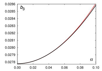
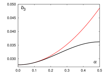
Figure 1: The third virial coefficient: black solid line — anyons; red dotted line — calculated. The upper panel corresponds to the close vicinity of the bosonic end while the lower one demonstrates the whole bosonic side $0\leq\alpha\leq 1/2$.

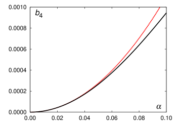
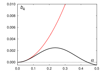
Figure 2: The fourth virial coefficient: black solid line — anyons; red dotted line — calculated. The upper panel corresponds to the close vicinity of the bosonic end while the lower one demonstrates the whole bosonic side $0\leq\alpha\leq 1/2$.

A natural question arises whether the obtained results affect the values of the fifth virial coefficient. For anyons, it equals in the bosonic limit [39]

$$b_{5}^{\rm anyon}\simeq-\frac{1}{3600}+0.0570337\alpha^{2}.$$ (17)

The above results reproducing the third and fourth virial coefficients yield the fifth virial coefficient shown in Fig. 3 compared to function (17).

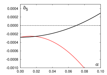
Figure 3: The fifth virial coefficient: black solid line — anyons; red dotted line — calculated.

One can easily notice that, except for an immediate vicinity of $\alpha=0$, the anyonic and calculated $b_{5}$ have opposite dependences on $\alpha$, just like it was observed in [34, 35] for the fourth virial coefficient.

It is possible to find such expressions for $f_{1,2}(\xi)$ demanding that expansions of virial coefficients $b_{2}$ through $b_{5}$ in $\alpha$ coincide with the anyonic results. In this case, $\ell_{\rm max}=4$ and we have a set of eight equations

linear in $\alpha$:	$b_{2}^{\rm anyon}=b_{2}$,  $b_{3}^{\rm anyon}=b_{3}$,  $b_{4}^{\rm anyon}=b_{4}$,  $b_{5}^{\rm anyon}=b_{5}$;
quadratic in $\alpha$:	$b_{2}^{\rm anyon}=b_{2}$,  $b_{3}^{\rm anyon}=b_{3}$,  $b_{4}^{\rm anyon}=b_{4}$,  $b_{5}^{\rm anyon}=b_{5}$.

The solutions are as follows:

$$k_{11}=a,\quad k_{12}=-0.6481\,a\quad k_{13}=0.3198\,a\quad k_{14}=0.04833\,a$$

$$k_{21}=b,\quad k_{22}=-1.4145\,b\quad k_{23}=0.7391\,b\quad k_{24}=-0.1321\,b$$ (18)

$$\textrm{with}\quad a=-\frac{71389}{2178}\simeq 32.78\quad\textrm{and}\quad b=-511.8.$$

So, the above values yield correct (up to $\alpha^{2}$) virial coefficients $b_{2}$ through $b_{5}$.

4 Fermionic limit

The fermionic limit corresponds to $\alpha^{\prime}=1-\alpha\to 0$. Technically, the calculations are similar to those for the bosonic case. The expansions of the virial coefficients in $\alpha^{\prime}$ are as follows:

$$b_{2}^{\rm anyon}=\phantom{-}\frac{1}{4}-\frac{1}{2}\alpha^{\prime\,2},$$ (19)

$$b_{3}^{\rm anyon}=\phantom{-}\frac{1}{36}+\frac{1}{12}\alpha^{\prime\,2},$$ (20)

$$b_{4}^{\rm anyon}\simeq-0.0149784\alpha^{\prime\,2}$$ (21)

Then, to find constants $k_{j\ell}$ one needs to equate coefficients near corresponding powers of $\alpha^{\prime}$ in expansions of anyonic virial coefficients and virial coefficients of the system under consideration.

At the fermionic end, obviously,

$$k_{1\ell}\equiv 0.$$ (22)

and in the second order

$$k_{21}\simeq-31.53,\quad k_{22}\simeq+26.35,\quad k_{23}\simeq-12.38.$$ (23)

These values yield correct (up to $\alpha^{2}$) virial coefficients $b_{2}$ through $b_{4}$ in the fermionic limit.

The results of calculations are compared to the virial coefficients of anyons in Figs. 4 and 5.

Figure 4: The third virial coefficient: black solid line — anyons; red dotted line — calculated. The upper panel corresponds to the close vicinity of the fermionic end while the lower one demonstrates the whole fermionic side $1/2\leq\alpha\leq 1$.

Figure 5: The fourth virial coefficient: black solid line — anyons; red dotted line — calculated. The upper panel corresponds to the close vicinity of the fermionic end while the lower one demonstrates the whole fermionic side $1/2\leq\alpha\leq 1$.

5 Effective excitation spectrum

Instead of deforming the Gibbs factor in the expression for the occupation numbers it is possible to consider the deformed spectrum $\epsilon_{\alpha}$. Indeed, comparing the following relations

$$\exp\left(\frac{\epsilon_{\alpha}}{T}\right)=X\left(\frac{\varepsilon}{T}\right)\equiv\exp\left(\frac{\varepsilon}{T}\right)\left[1+\alpha f_{1}\left(\frac{\varepsilon}{T}\right)+\alpha^{2}f_{2}\left(\frac{\varepsilon}{T}\right)\right]$$ (24)

we easily obtain the spectrum in the $\alpha^{2}$ approximation:

$$\epsilon_{\alpha}=\varepsilon\left\{1+\alpha f_{1}\left(\frac{\varepsilon}{T}\right)+\alpha^{2}\left[f_{2}\left(\frac{\varepsilon}{T}\right)-\frac{1}{2}f_{1}^{2}\left(\frac{\varepsilon}{T}\right)\right]\right\}.$$ (25)

Energy $\varepsilon$ corresponds, e. g., to $\varepsilon_{j}=\hbar\omega j$ for harmonically trapped anyons or to $\varepsilon_{k}=\hbar^{2}k^{2}/(2m)$ for free anyons. The correction to the spectrum is shown in Fig. 6.

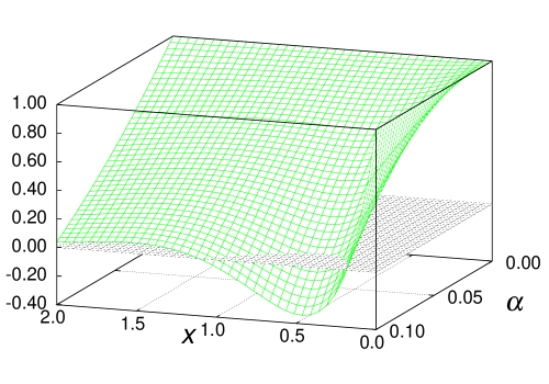
Figure 6: The spectrum correction $\displaystyle\frac{\epsilon_{\alpha}}{\varepsilon}$ for the anyonic parameter $0\leq\alpha\leq 0.1$ and argument $\displaystyle 0\leq\frac{\varepsilon}{T}\leq 2$.

Such an effective spectrum can be used to model anyons using expressions for occupation numbers within the ordinary Bose and Fermi statistics in the appropriate limits.

6 Discussion

We have made an attempt to define a functional form for the occupation numbers of free anyons. Previous models corresponded to exact results for the second and third virial coefficients with a difference only in the fourth virial coefficient leading to a small correction in the equation of state. The approach of the present work reproduces both the fourth and higher virial coefficients in the limits of the Bose and Fermi statistics by means of a deformation of the Gibbs factor in the standard Bose and Fermi distributions, respectively.

We further plan to juxtapose the obtained statistical-mechanical description and quantum-mechanical models based on modifications of commutation relations or special algebra for creation–annihilation operators. Extensions of the discussed approach for interaction anyons is also expected.

References

- [1] J. M. Leinaas and J. Myrheim. On the theory of identical particles. Nuovo Cim., 37B(1):1–23, 1977.
- [2] F. Wilczek. Quantum mechanics of fractional-spin particles. Phys. Rev. Lett., 49(14):957–959, 1982.
- [3] D. C. Tsui, H. L. Stormer, and A. C. Gossard. Two-dimensional magnetotransport in the extreme quantum limit. Phys. Rev. Lett., 48(22):1559–1562, 1982.
- [4] R. B. Laughlin. Anomalous quantum Hall effect: An incompressible quantum fluid with fractionally charged excitations. Phys. Rev. Lett., 50(18):1395–1398, 1983.
- [5] B. I. Halperin. Statistics of quasiparticles and the hierarchy of fractional quantized Hall states. Phys. Rev. Lett., 52(18):1583–1586, 1984.
- [6] D. Arovas, J. R. Schrieffer, and F. Wilczek. Fractional statistics and the quantum Hall effect. Phys. Rev. Lett., 53(7):722–723, 1984.
- [7] Bing-Shen Wang, Joseph L Birman, and Zhao-Bin Su. Optical spectrum of 2d electrons in the fractional quantum hall regime. Phys. Rev. Lett., 68(10):1605, 1992.
- [8] F. E. Camino, W. Zhou, and V. J. Goldman. Realization of a Laughlin quasiparticle interferometer: Observation of fractional statistics. Phys. Rev. B, 72(7):075342, 2005.
- [9] Jimmy A. Hutasoit, Ajit C. Balram, Sutirtha Mukherjee, Ying-Hai Wu, Sudhansu S. Mandal, A. Wójs, Vadim Cheianov, and J. K. Jain. The enigma of the fractional quantum Hall effect. Phys. Rev. B, 95:125302, Mar 2017.
- [10] Roger S. K. Mong, Michael P. Zaletel, Frank Pollmann, and Zlatko Papić. Fibonacci anyons and charge density order in the 12/5 and 13/5 quantum hall plateaus. Phys. Rev. B, 95(11):115136, 2017.
- [11] Cheolhee Han, Jinhong Park, Yuval Gefen, and H.-S. Sim. Topological vacuum bubbles by anyon braiding. Nature Commun., 7, 2016.
- [12] A. Braggio, M. Carrega, D. Ferraro, and M. Sassetti. Finite frequency noise spectroscopy for fractional hall states at . J. Stat. Mech.: Theor. Exp., 2016(5):054010, 2016.
- [13] Jérôme Rech, Dario Ferraro, Thibaut Jonckheere, Luca Vannucci, Maura Sassetti, and Thierry Martin. Minimal excitations in the fractional quantum hall regime. Phys. Rev. Lett., 118(7):076801, 2017.
- [14] C. N. Yang and M. L. Ge. Braid Group, Knot Theory, and Statistical Mechanics II, volume II. World Scientific Publishing Co. Pte. Ltd., Singapore, 1994.
- [15] C. Weeks, G. Rosenberg, B. Seradjeh, and M. Franz. Anyons in a weakly interacting system. Nature Phys., 3:797–801, 2007.
- [16] Michael H. Freedman, Alexei Kitaev, and Zhenghan Wang. Simulation of topological field theories by quantum computers. Commun. Math. Phys., 227(3):587–603, 2002.
- [17] A. P. Polychronakos. Virial coefficients of non-Abelian anyons. Phys. Rev. Lett., 84(6):1268–1271, 2000.
- [18] Yi-Zhuang You, Chao-Ming Jian, and Xiao-Gang Wen. Synthetic non-Abelian statistics by Abelian anyon condensation. Phys. Rev. B, 87(4):045106, 2013.
- [19] F. Mancarella, A. Trombettoni, and G. Mussardo. Statistical mechanics of an ideal gas of non-Abelian anyons. Nucl. Phys. B, 867 [FS]:950–976, 2013.
- [20] Simon Burton, Courtney G. Brell, and Steven T. Flammia. Classical simulation of quantum error correction in a fibonacci anyon code. Phys. Rev. A, 95:022309, Feb 2017.
- [21] Keren Li, Yidun Wan, Ling-Yan Hung, Tian Lan, Guilu Long, Dawei Lu, Bei Zeng, and Raymond Laflamme. Experimental identification of non-abelian topological orders on a quantum simulator. Phys. Rev. Lett., 118:080502, Feb 2017.
- [22] Christina Knapp, Michael Zaletel, Dong E. Liu, Meng Cheng, Parsa Bonderson, and Chetan Nayak. The nature and correction of diabatic errors in anyon braiding. Phys. Rev. X, 6:041003, 2016.
- [23] Matthew F. Lapa, Gil Young Cho, and Taylor L. Hughes. Bosonic analog of a topological dirac semimetal: Effective theory, neighboring phases, and wire construction. Phys. Rev. B, 94:245110, 2016.
- [24] Alexandre M. Gavrilik and Ivan I. Kachurik. Nonstandard deformed oscillators from - and -deformations of Heisenberg algebra. SIGMA, 12:047, 2016.
- [25] A. Khare. Fractional Statistics and Quantum Theory. World Scientific, Singapore, 2nd edition, 2005.
- [26] S. L. Dalton and A. Inomata. Anyonic quon gas. Phys. Lett. A, 199:315–319, 1995.
- [27] A. Algin, M. Arik, and A. S. Arikan. High temperature behavior of a two-parameter deformed quantum group fermion gas. Phys. Rev. E, 65(2):026140, 2002.
- [28] A. Algin. Fibonacci oscillators and two-parameter generalized thermostatistics. Commun. Nonlinear Sci. Numer. Simulat., 15:1372–1377, 2010.
- [29] A. M. Gavrilik and Yu. A. Mishchenko. Deformed Bose gas models aimed at taking into account both compositeness of particles and their interaction. Ukr. J. Phys., 58(12):1171–1177, 2013.
- [30] A. P. Polychronakos. Probabilities and path-integral realization of exclusion statistics. Phys. Lett. B, 365:202–206, 1996.
- [31] F. D. M. Haldane. “Fractional statistics” in arbitrary dimension: A generalization of the Pauli principle. Phys. Rev. Lett., 67(8):937–940, 1991.
- [32] Y.-S. Wu. Statistical distribution for generalized ideal gas of fractional-statistics particles. Phys. Rev. Lett., 73(7):922–925, 1994.
- [33] C. Tsallis. Possible generalization of Boltzmann-Gibbs statistics. J. Stat. Phys., 52(1–2):479–486, 1988.
- [34] A. Rovenchak. Two-parametric fractional statistics models for anyons. Eur. Phys. J. B, 87(8):175, 2014.
- [35] M. Ya. Hornetska and A. A. Rovenchak. Two-parameter modifications of anyonic statistics. Ukr. J. Phys., 61(2):168–177, 2016.
- [36] S. Mashkevich, J. Myrheim, and K. Olaussen. The third virial coefficient of anyons revisited. Phys. Lett. B, 382:124–130, 1996.
- [37] A. Kristoffersen, S. Mashkevich, J. Myrheim, and K. Olaussen. The fourth virial coefficient of anyons. Int. J. Mod. Phys. A, 13(21):3723–3747, 1998.
- [38] P. F. Borges, H. Boschi-Filho, and C. Farina. Generalized partition functions, interpolating statistics and higher virial coefficients. Mod. Phys. Lett. A, 14(18):1217–1226, 1999.
- [39] A. Dasnières de Veigy and S. Ouvry. Perturbative equation of state for a gas of anyons. Second order. Phys. Lett. B, 291(1–2):130–136, 1992.