Quantum and thermal fluctuations in a Raman spin-orbit coupled Bose gas

Abstract

We theoretically study a three-dimensional weakly-interacting Bose gas with Raman-induced spin-orbit coupling at finite temperature. By employing a generalized Hartree-Fock-Bogoliubov theory with Popov approximation, we determine a complete finite-temperature phase diagram of three exotic condensation phases (i.e., the stripe, plane-wave and zero-momentum phases), against both quantum and thermal fluctuations. We find that the plane-wave phase is significantly broadened by thermal fluctuations. The phonon mode and sound velocity at the transition from the plane-wave phase to the zero-momentum phase are thoughtfully analyzed. At zero temperature, we find that quantum fluctuations open an unexpected gap in sound velocity at the phase transition, in stark contrast to the previous theoretical prediction of a vanishing sound velocity. At finite temperature, thermal fluctuations continue to significantly enlarge the gap, and simultaneously shift the critical minimum. For a Bose gas of ⁸⁷Rb atoms at the typical experimental temperature, $T=0.3T_{0}$, where $T_{0}$ is the critical temperature of an ideal Bose gas without spin-orbit coupling, our results of gap opening and critical minimum shifting in the sound velocity, are qualitatively consistent with the recent experimental observation [S.-C. Ji et al., Phys. Rev. Lett. 114, 105301 (2015)].

The interaction of a particle’s spin with its spatial motion - the so-called spin-orbit coupling (SOC) - plays an important role in various areas of physics. Over the past few years, the SOC effects have been under extensive studies in alkali atomic quantum gases Dalibard2011 ; Galitski2013 ; Goldman2014 ; Zhai2015 , owing to the high controllability of cold-atom platforms Bloch2008 . By utilizing two counter-propagating Raman lasers via a two-photon process, physicists have realized one-dimensional SOC with an equal weight combination of Rashba and Dresselhaus types, which couples two atomic internal states Lin2011 ; Wang2012 ; Cheuk2012 . Most recently, two-dimensional SOC of Rashba type is also achieved Huang2016 ; Wu2016 . These seminal breakthroughs lead to fruitful researches both theoretically Wang2010 ; Wu2011 ; Ho2011 ; Hu2012 ; Li2012PRL ; Li2012EPL ; Ozawa2012PRA ; Martone2012 ; Zheng2012 ; Ozawa2012PRL ; Zheng2013 ; Yu2013 ; Chen2017 and experimentally Zhang2012 ; Ji2014 ; Ji2015 ; Li2017 , giving rise to many fascinating phenomena, such as the exotic bosonic superfluidity Wang2010 ; Wu2011 ; Ho2011 ; Hu2012 ; Li2012PRL ; Yu2013 , topological superfluidity and Majorana fermions Sato2009 ; Jiang2011 ; Liu2012a ; Liu2012b ; Liu2013 ; Liu2014 , and the spin Hall effect Zhu2006 ; Liu2007 ; Beeler2013 .

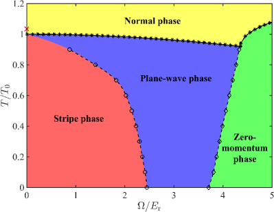
Figure 1: (color online). Phase diagram of a two-component Bose gas with Raman induced spin-orbit coupling in the plane of temperature $T$ and Raman Rabi frequency $\Omega$. The temperature is measured in units of the critical BEC temperature of an ideal spinless Bose gas with density $n/2$, i.e., $T_{0}=2\pi\hbar^{2}[(n/2)/\zeta(3/2)]^{2/3}/(mk_{B})$. We take the total density of our SOC Bose gas, $n=1.0k_{\textrm{r}}^{3}$, the intra-species interaction energy, $gn=0.8E_{\textrm{r}}$, and the inter-species interaction energy, $g_{{}_{\uparrow\downarrow}}n=0.5E_{\textrm{r}}$. Here, $k_{\textrm{r}}$ and $E_{\textrm{r}}=\hbar^{2}k_{\textrm{r}}^{2}/(2m)$ are Raman wave-vector and the recoil energy, respectively.

In this Rapid Communication, we are interested in a three-dimensional weakly interacting Bose gas with a one-dimensional SOC at finite temperature. The zero-temperature phase diagram of such a Bose gas was explored in detail in last few years Lin2011 ; Ho2011 ; Li2012PRL ; Ozawa2012PRA ; Martone2012 ; Zheng2013 , by using the Gross-Pitaevskii (GP) equation and the Bogoliubov theory. There are typically three exotic phases by tuning the Rabi frequency of the two Raman beams (see Fig. 1 at $T=0$): the stripe (ST) phase, the plane-wave (PW) phase and the zero-momentum (ZM) phase Lin2011 ; Ho2011 . Only a handful of theoretical investigations have addressed the finite-temperature effects so far Ozawa2012PRL ; Yu2014 , which are however unavoidable in realistic experiments Ji2014 ; Ji2015 . Theoretically, Ozawa and Baym discussed the stability of condensates against quantum and thermal fluctuations Ozawa2012PRL . Experimentally, by measuring the magnetization of the condensate of ⁸⁷Rb atoms, Ji et al. determined a qualitative finite-temperature phase diagram of the ST-PW transition Ji2014 . A follow-up theoretical study by Yu perturbatively calculated the ST-PW boundary at finite temperature in terms of small Rabi frequency, and obtained a good agreement Yu2014 . Unfortunately, this perturbation approach fails at relatively high temperature, and also is not applicable for a large difference in intra- and inter-species interaction strengths, which leads to a large critical Rabi frequency Li2012PRL ; Li2017 . Furthermore, the phase transition from the PW phase to the ZM phase in the presence of quantum and thermal fluctuations has not been explored both theoretically and experimentally. The purpose of our work is to present a solid calculation of a SOC Bose gas at finite temperature, by developing a self-consistent Hartree-Fock-Bogoliubov theory within Popov approximation. In this way, we address the quantum and thermal effects on different condensation phases.

Our main results are briefly summarized in Fig. 1, where we delineate a finite-temperature phase diagram on Raman Rabi frequency (the horizontal axis) and nonzero temperature (the vertical axis). Four distinct regimes could be clearly identified: the ST phase (red), PW phase (blue), ZM phase (green) and normal phase (yellow). We find that, by increasing temperature, the PW phase is significantly enlarged before reaching the superfluid-to-normal phase transition. In addition to confirming the previous perturbative prediction by Yu Yu2014 , our results clearly reveal that the PW-ZM boundary is significantly shifted by nonzero temperature, in sharp contrast to the naive picture drawn earlier Ji2014 . This shift is also found in the sound velocity, which exhibits a minimum at the PW-ZM transition (see Fig. 4). Therefore, it can be experimentally measured by using Bragg spectroscopy. Indeed, for ⁸⁷Rb atoms, our calculation with a realistic temperature indicates a sizable shift in the sound velocity minimum, consistent with the recent experimental measurement Ji2015 (see the inset of Fig. 4).

Model. A two-component Bose gas with Raman induced spin-orbit coupling can be well described by the model Hamiltonian, $\hat{H}=\hat{H}_{0}+\hat{H}_{\textrm{int}}$ Li2012PRL ; Martone2012 ; Zheng2013 , where the single-particle Hamiltonian is ($\hbar=1$)

$$\hat{H}_{0}=\int\mathrm{d}^{3}\mathbf{r}\left[\hat{\Phi}_{\uparrow}^{\dagger}(\mathbf{r}),\hat{\Phi}_{\downarrow}^{\dagger}(\mathbf{r})\right]\mathcal{H}_{s}(\hat{{\bf p}})\left[\begin{array}[]{c}\hat{\Phi}_{\uparrow}(\mathbf{r})\\ \hat{\Phi}_{\downarrow}(\mathbf{r})\end{array}\right],$$ (1)

with $\mathcal{H}_{s}(\hat{{\bf p}})=(\hat{{\bf p}}-k_{\textrm{r}}\mathbf{e}_{x}\sigma_{z})^{2}/(2m)+(\Omega\sigma_{x}+\delta\sigma_{z})/2$ and $\hat{{\bf p}}=-i\mathbf{\nabla}$, and the interaction Hamiltonian is

$$\hat{H}_{\textrm{int}}=\frac{1}{2}\int\mathrm{d}^{3}\mathbf{r}\sum_{\sigma,\sigma^{\prime}=\uparrow\downarrow}g_{\sigma\sigma^{\prime}}\hat{\Phi}_{\sigma}^{\dagger}\hat{\Phi}_{\sigma^{\prime}}^{\dagger}\hat{\Phi}_{\sigma^{\prime}}\hat{\Phi}_{\sigma}(\mathbf{r}),$$ (2)

with $g_{\sigma\sigma^{\prime}}=4\pi a_{\sigma\sigma^{\prime}}/m$. Here, $\Omega$ and $\delta$ are respectively the Rabi frequency and detuning of the Raman lasers, $\sigma_{x}$ and $\sigma_{z}$ are Pauli matrices, and $a_{\sigma\sigma^{\prime}}$ are the intra- ($\sigma=\sigma^{\prime}$) and inter-species ($\sigma\neq\sigma^{\prime}$) $s$-wave scattering lengths. The recoil momentum $\mathbf{k}=k_{\textrm{r}}\mathbf{e}_{x}$ of the laser beams is along the $x$-axis and the corresponding recoil energy is $E_{\textrm{r}}=k_{\textrm{r}}^{2}/(2m)$. For ⁸⁷Rb atoms, the SOC term $\hat{p}_{x}\sigma_{z}k_{\textrm{r}}/m$ in $\mathcal{H}_{s}(\hat{{\bf p}})$ describes a momentum-dependent coupling between hyperfine states in the $F=1$ ground state manifold Lin2011 . Following the typical experimental parameters Ji2014 ; Ji2015 , we assume a zero laser detuning, $\delta=0$, and the interaction strengths $g_{\uparrow\uparrow}=g_{\downarrow\downarrow}=g\neq g_{\uparrow\downarrow}$.

Hartree-Fock-Bogoliubov-Popov theory. To describe quantum and thermal fluctuations, we generalize a Hartree-Fock-Bogoliubov theory Griffin1996 ; Dodd1998 ; Buljan2005 within Popov approximation PopovBook (HFBP) and apply it to the SOC Bose gas. Following the standard procedure Chen2015 , we separate the Bose field operator $\hat{\Phi}({\bf r},t)$ into a combination of condensate wave-functions $\phi_{\sigma}(\mathbf{r})$ and the fluctuation operators $\hat{\eta_{\sigma}}(\mathbf{r},t)$ as ($\sigma=\uparrow,\downarrow$),

$$\left[\begin{array}[]{c}\hat{\Phi}_{\uparrow}\\ \hat{\Phi}_{\downarrow}\end{array}\right]=e^{-i\mu t}e^{iP_{x}x}\left[\sqrt{n_{c}}\left(\begin{array}[]{c}\cos\theta\\ -\sin\theta\end{array}\right)+\left(\begin{array}[]{c}\hat{\eta}_{\uparrow}\\ \hat{\eta}_{\downarrow}\end{array}\right)\right],$$ (3)

with the chemical potential $\mu$ and a uniform density $n_{c}=N_{c}/V$ Li2012PRL ; Martone2012 ; Zheng2013 . For simplicity, in this work we focus on a plane-wave wave-function for the condensate moving along the $x$-direction with the momentum $P_{x}\geq 0$. We also use an angle $\theta$ in the range $[0,\pi/4]$ to weight the spin-up and spin-down condensate components. Both variational parameters, $\theta$ and $P_{x}$, are to be determined by minimizing the free energy of the system. The fluctuation operators $\hat{\eta}_{\sigma}$ and their conjugate can be expanded in a quasiparticle basis ($\hat{a}^{\dagger}$, $\hat{a}$) under a Bogoliubov transformation, i.e., $\hat{\eta}_{\sigma}(\mathbf{r},t)=\sum_{j}[u_{j\sigma}({\bf r})e^{-i\omega_{j}t}\hat{a}_{j}+v_{j\sigma}^{*}({\bf r})e^{i\omega_{j}t}\hat{a}_{j}^{\dagger}]$, where in the uniform case the quasiparticle amplitudes may take the form, $u_{j\sigma}({\bf r})=u_{{\bf q}\sigma}^{(\tau)}\mathrm{exp}(i{\bf q\cdot r})$ and $v_{j\sigma}({\bf r})=v_{{\bf q}\sigma}^{(\tau)}\mathrm{exp}(i{\bf q\cdot r})$, and the index $j=(\mathbf{q},\tau=\pm)$ of the quasiparticle energy levels can be represented by the momentum $\mathbf{q}$ and the helicity branch index $\tau=\pm$ due to the SOC Cao2014 .

By substituting the Bose field operators Eq. (3) into the equations of motion $i\partial_{t}\hat{\Phi}_{\sigma}({\bf r},t)=[\hat{\Phi}_{\sigma},\hat{H}]$, taking the standard mean-field decoupling (i.e., Hartree-Fock-Bogoliubov approximation) Griffin1996 , and omitting the terms with anomalous densities $n_{a}=\langle\hat{\eta}_{\sigma}\hat{\eta}_{-\sigma}\rangle$ (i.e., Popov approximation) PopovBook ; Chen2015 , we obtain two separate equations for the condensate and Bogoliubov quasiparticles, respectively: (i) the modified GP equations,

$$\left[\mathcal{H}_{s}(\hat{{\bf p}})+\mathrm{diag}(\mathcal{L}_{\uparrow},\mathcal{L}_{\downarrow})\right]\phi=\mu\phi,$$ (4)

with $\phi=(\phi_{\uparrow},\phi_{\downarrow})^{T}$ and $\mathcal{L}_{\sigma}\equiv g(n_{c\sigma}+2n_{t\sigma})+g_{{}_{\uparrow\downarrow}}n_{-\sigma}$, and (ii) the generalized Bogoliubov equations,

$$\left[\mathcal{H}_{s}\left(\hat{{\bf p}}+{\bf q}\right)-\mu+\mathcal{A}_{\uparrow}\right]U_{\mathbf{q}}^{(\tau)}+\mathcal{B}V_{\mathbf{q}}^{(\tau)} = \varepsilon_{\mathbf{q\tau}}U_{\mathbf{q}}^{(\tau)},$$ (5)

$$-\mathcal{B}U_{\mathbf{q}}^{(\tau)}-\left[\mathcal{H}_{s}\left(\hat{{\bf p}}-{\bf q}\right)-\mu+\mathcal{A}_{\downarrow}\right]V_{\mathbf{q}}^{(\tau)} = \varepsilon_{\mathbf{q}\tau}V_{\mathbf{q}}^{(\tau)},$$ (6)

where $U_{{\bf q}}^{(\tau)}=[u_{{\bf q}\uparrow}^{(\tau)},u_{{\bf q}\downarrow}^{(\tau)}]^{T}$, $V_{{\bf q}}^{(\tau)}=[v_{{\bf q}\uparrow}^{(\tau)},v_{{\bf q}\downarrow}^{(\tau)}]^{T}$, and

$$\mathcal{A}_{\sigma} \equiv \left[\begin{array}[]{cc}2gn_{\sigma}+g_{{}_{\uparrow\downarrow}}n_{-\sigma}&g_{{}_{\uparrow\downarrow}}\phi_{\sigma}\phi_{-\sigma}\\ g_{{}_{\uparrow\downarrow}}\phi_{\sigma}\phi_{-\sigma}&2gn_{-\sigma}+g_{{}_{\uparrow\downarrow}}n_{\sigma}\end{array}\right],$$ (9)

$$\mathcal{B} \equiv \left[\begin{array}[]{cc}g\phi_{\uparrow}^{2}&g_{{}_{\uparrow\downarrow}}\phi_{\uparrow}\phi_{\downarrow}\\ g_{{}_{\uparrow\downarrow}}\phi_{\uparrow}\phi_{\downarrow}&g\phi_{\downarrow}^{2}\end{array}\right].$$ (12)

Here, $n_{c\uparrow}=n_{c}\cos^{2}\theta$ and $n_{c\downarrow}=n_{c}\sin^{2}\theta$ are the condensate density of the two components, $n_{t\sigma}\equiv\langle\hat{\eta}_{\sigma}^{\dagger}\hat{\eta}_{\sigma}\rangle=(1/V)\sum_{{\bf q\tau}}[(|u_{{\bf q}\sigma}^{(\tau)}|^{2}+|v_{{\bf q}\sigma}^{(\tau)}|^{2})/(e^{\beta\varepsilon_{\mathbf{q\tau}}}-1)+|v_{{\bf q}\sigma}^{(\tau)}|^{2}]$ with $\beta\equiv 1/(k_{B}T)$ and $n_{\sigma}=n_{c\sigma}+n_{t\sigma}$ are the non-condensate density and the total density for spin $\sigma$, respectively. We note that, the generalized Bogoliubov equations give rise to four solutions with energies $\pm\varepsilon_{\mathbf{q},\tau=\pm}$. We retain the two physical solutions with positive energies $\varepsilon_{\mathbf{q},\tau=\pm}>0$ only. Note also that, in all the previous studies, the non-condensate density $n_{t\sigma}$ is neglected Li2012PRL ; Martone2012 ; Zheng2013 . This treatment is reasonable at zero temperature, where the quantum depletion $n_{t\sigma}^{(\textrm{Q})}=(1/V)\sum_{{\bf q\tau}}|v_{{\bf q}\sigma}^{(\tau)}|^{2}\sim 0.01n_{{}_{\sigma}}$ is typically small in the weak-coupling regime. However, as we shall see, near the phase transition the small quantum depletion may lead to qualitative changes to some experimental observables such as sound velocity.

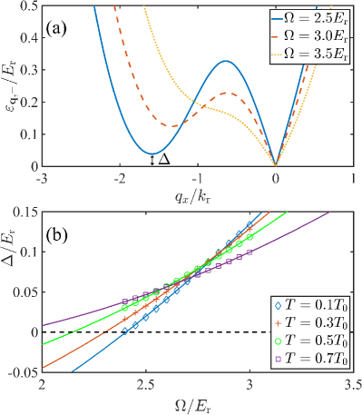
Figure 2: (color online). (a) The Bogoliubov excitation spectra $\varepsilon_{\mathbf{q},\tau=-}$ at temperature $T=0.4T_{0}$ and at various Rabi frequencies. Here, we set $q_{{}_{y}}=q_{z}=0$. The roton gap at $\Omega=3.5E_{\textrm{r}}$ is explicitly indicated. (b) The roton gap $\Delta$ as a function of Rabi frequency $\Omega$ at different temperatures, fitted with second-order polynomials (solid lines).

Once the generalized GP and Bogoliubov equations are self-consistently solved at finite temperature for a given set of variational parameters ($\theta,P_{x}$) note1 , we calculate straightforwardly the free energy of the system, $\mathcal{F}(\theta,P_{x})/V=\mu n+\Omega_{G}/V$, where the grand potential per volume is given by PitaevskiiStringariSBook ; FetterWaleckaBook ,

$$\frac{\Omega_{G}}{V}=(E_{0}-\mu)n_{c}+\frac{k_{B}T}{V}\sum_{{\bf q},\tau=\pm}\ln(1-e^{-\beta\varepsilon_{{\bf q}\tau}})$$ (13)

and the condensate energy per particle is $E_{0}(\theta,P_{x})=(P_{x}^{2}+k_{\textrm{r}}^{2}-2P_{x}k_{\textrm{r}}\cos{2\theta})/(2m)+(gn_{c}-\Omega\sin{2\theta})/2-(g-g_{{}_{\uparrow\downarrow}})n_{c}\sin^{2}\theta\cos^{2}\theta$ Li2012PRL ; Martone2012 . The two variational parameters $\theta$ and $P_{x}$ are determined by minimizing the free energy $\mathcal{F}$:

$$\left(\frac{\partial\mathcal{F}}{\partial\theta}\right)_{N}=0,~{}~{}\left(\frac{\partial\mathcal{F}}{\partial P_{x}}\right)_{N}=0.$$ (14)

At zero temperature, under the approximation of negligible quantum depletion (i.e., $n_{c}=n$), we have $\mathcal{F}=E_{0}(\theta,P_{x})nV$, so the minimization can be carried out analytically Li2012PRL ; Martone2012 ; Zheng2013 . For ⁸⁷Rb atoms with the interaction energies lengths $gn=0.38E_{\textrm{r}}$ and $g_{{}_{\uparrow\downarrow}}/g=100.99/101.20$ at typical density $n=0.46k_{\textrm{r}}^{3}$ Ji2015 , this minimization leads to two critical Rabi frequencies, $\Omega_{c1}\simeq 0.2E_{\textrm{r}}$ and $\Omega_{c2}\simeq 4.0E_{\textrm{r}}$, which locate the first-order ST-PW and second-order PW-ZM transitions at zero temperature, respectively Lin2011 ; Ji2014 ; Ji2015 . The phase space for the stripe phase is therefore very narrow Ji2014 . To amplify the interaction effects on the phase diagram, in all our numerical calculations, we use a total density $n=1.0k_{\textrm{r}}^{3}$, the interaction energies $gn=0.8E_{\textrm{r}}$ and $g_{{}_{\uparrow\downarrow}}n=0.5E_{\textrm{r}}$. The relatively large difference in the intra- and inter-species interaction strengths gives rise to a more experimentally accessible critical Rabi frequency $\Omega_{c1}\simeq 2.4E_{\textrm{r}}$ at $T=0$. We note that, in the latest experiment on SOC Bose gases, where the two spin-components are realized by two low-lying bands in a superlattice, the interaction energy $g_{{}_{\uparrow\downarrow}}n$ can be tuned at will by controlling the overlap in wave-functions of the two bands, leading to a large phase space for the stripe phase with $\Omega_{c1}\simeq 1.5E_{\textrm{r}}$ Li2017 .

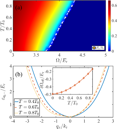
Figure 3: (color online). (a) The contour plot of the condensate-momentum $P_{x}$, in units of $k_{\textrm{r}}$, as functions of $T$ and $\Omega$. The boundary $P_{x}=0$ between PW and ZM phases is highlighted by the white dashed line. (b) The Bogoliubov excitation spectra $\varepsilon_{\mathbf{q},\tau=-}$ at various temperatures, with $q_{{}_{x}}=q_{y}=0$. The inset shows the temperature dependence of the effective Rabi frequency $\delta\Omega_{\textrm{eff}}=2g_{\uparrow\downarrow}\phi_{\uparrow}\phi_{\downarrow}$. Here, we take $\Omega=4.0E_{\textrm{r}}$.

Phase diagram. We are now ready to address the finite temperature effects on the ST-PW and PW-ZM phase transitions. An intriguing feature of the PW phase is the emergence of the roton-maxon structure in the lowest-lying Bogoliubov excitation spectrum Zheng2012 ; Martone2012 ; Zheng2013 , as reported in Fig. 2(a) at a nonzero temperature $T=0.4T_{0}$, where $T_{0}=2\pi\hbar^{2}[(n/2)/\zeta(3/2)]^{2/3}/(mk_{B})$ is the critical temperature of an ideal Bose gas with density $n/2$ in the absence of SOC. This structure becomes much more pronounced with decreasing Rabi frequency $\Omega$ and can be quantitatively characterized by a roton gap $\Delta$, as indicated in Fig. 2(a). Toward the ST-PW transition, the roton gap is gradually softened and approaches zero precisely at the transition. Therefore, as shown in Fig. 2(b), we determine the critical Rabi frequency $\Omega_{c1}$ from the $\Omega$-dependence of the roton gap. As the accuracy of our numerical calculations becomes worse near the transition, we typically fit the data by using a second-order polynomial note2 and then calculate $\Omega_{c1}$ from the fitting curve. By repeating this procedure at different temperatures, we obtain the temperature dependence of the ST-PW boundary, as shown in Fig. 1 by the empty circles.

On the other hand, we can straightforwardly determine the PW-ZM transition by identifying the critical Rabi frequency $\Omega_{c2}$, at which the condensate momentum $P_{x}$ approaches zero. This is illustrated in the contour plot Fig. 3(a) on the $T$-$\Omega$ plane, where the transition is highlighted by the white dashed line (see also the empty diamonds in Fig. 1). Furthermore, in Fig. 3(b), we check the temperature dependence of the lowest-lying Bogoliubov excitation spectrum at $\Omega=4.0E_{\textrm{r}}$. By increasing temperature from $0.4T_{0}$ to $0.6T_{0}$, and then to $0.8T_{0}$, the spectrum changes from a symmetric shape (with respect to $q_{x}=0$) to an asymmetric one. An asymmetric phonon dispersion near $q_{x}=0$ is another characteristic feature of the PW phase. It leads to different sound velocities when a density fluctuation propagates along or opposite to the positive $x$-axis, which we shall discuss in detail later.

From the phase diagram Fig. 1, it is evident that the phase space of the PW phase is greatly enlarged by temperature or thermal fluctuations. The stripe phase is not energetically favorable at relatively large temperature, as anticipated. As mentioned earlier, the stripe phase is driven by the difference in the intra- and inter-species interaction energies, i.e., $gn_{c}$ and $g_{\uparrow\downarrow}n_{c}$. This difference becomes increasingly smaller with increasing temperature, since the condensate density decreases. Hence, the stripe phase shrinks. Our HFBP finding is consistent with the previous experimental determination of the ST-PW boundary with ⁸⁷Rb atoms at nonzero temperature Ji2014 , and it also provides a useful microscopic confirmation of the perturbative theory by Yu Yu2014 . In contrast, the significant shrinkage of the ZM phase at finite temperature - observed as well with parameters for ⁸⁷Rb atoms - is entirely not expected (see, for example, the naive phase diagram sketched in Ref. Ji2014 ). Recall that the PW-ZM transition is largely due to the change of the single-particle dispersion with increasing Rabi frequency Lin2011 ; Li2012PRL . From the mean-field point of view, therefore, the notable shift of the PW-ZM boundary suggests a strong temperature dependence of the effective Rabi frequency $\delta\Omega_{\textrm{eff}}\equiv 2g_{{}_{\uparrow\downarrow}}\phi_{\uparrow}\phi_{\downarrow}=-g_{\uparrow\downarrow}n_{c}\sin 2\theta$, which is resulted from the inter-species interaction (see Eqs. (5), (6) and (9)). Indeed, as shown in the inset of Fig. 3(b), such a sensitive temperature dependence is confirmed at a typical Rabi frequency $\Omega=4.0E_{\textrm{r}}$.

At high temperature, the SOC Bose gas becomes normal. Unfortunately, sufficiently close to the superfluid-normal phase transition, our HFBP theory becomes less accurate Griffin1996 . To determine the transition temperature, we follow the previous work by Zheng et al. and adopt the Hartree-Fock approximation Zheng2013 . The resulting critical temperature $T_{c}$ is shown at the top of Fig. 1 by a solid curve with asterisks. At small Rabi frequency, the predicted $T_{c}$ differs slightly from the classical Monte Carlo simulation Arnold2001 ; Kashurnikov2001 (red cross), which confirmed a linear shift of $T_{c}$ in the s-wave scattering length $\Delta T_{c}/T_{0}\approx 1.3n^{1/3}a$. At large Rabi frequency (i.e., $\Omega>4E_{\textrm{r}}$), it is interesting that the Hartree-Fock transition temperature matches very well with the PW-ZM boundary. This is a strong indication that our HFBP predictions might be reliable at temperature $T<0.9T_{0}$.

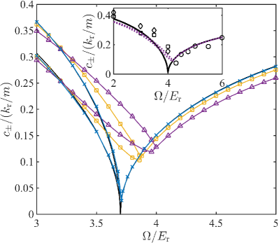
Figure 4: (color online) Sound velocities $c_{+}$ and $c_{-}$ as a function of Rabi frequency $\Omega$ at $T=0$ (black lines - without quantum fluctuations; blue lines with crosses - with quantum fluctuations), $T=0.2T_{0}$ (yellow lines with squares), and $T=0.4T_{0}$ (purple lines with triangles). The inset shows the sound velocities in a ⁸⁷Rb SOC gas at $T=0$ (black lines) and $T=0.3T_{0}$ (purple dotted lines). The symbols are the experimental data Ji2015 . To simulate the experiment, we take a total density $n=0.46k_{\textrm{r}}^{3}$, $gn=0.38E_{\textrm{r}}$ and $g_{{}_{\uparrow\downarrow}}/g=100.99/101.20$.

Sound velocities. We now turn to discuss in greater detail the anisotropic phonon dispersion at small $q_{x}$ in the PW phase and the resulting two sound velocities $c_{+}>c_{-}$ Li2012PRL ; Martone2012 ; Zheng2013 , which have been measured experimentally to characterize the PW-ZM transition Ji2015 . Note that, turning into the ZM phase the two velocities would merge into one, i.e., $c_{+}=c_{-}\equiv c$ Li2012PRL ; Martone2012 ; Zheng2013 .

In Fig. 4, we report the behavior of sound velocities across the PW-ZM transition as a function of Rabi frequency at various temperatures. At zero temperature, all the previous studies predicted a vanishing velocity right at the transition point $\Omega_{c2}$. Physically, since the sound velocity may be well approximated by $c\simeq\sqrt{gn/m_{\mathrm{eff}}}$, the vanishing sound velocity is a consequence of the flatness of the single-particle spectrum at the transition and hence a divergent effective mass $m_{\textrm{eff}}\rightarrow\infty$ Martone2012 ; Zheng2013 . This interesting feature is exactly produced by our numerical calculation if we do not account for the feedback of quantum fluctuations to the total density (see the black solid curve). However, once we take into account quantum fluctuations, there is a qualitatively change. Although the sound velocities still exhibit a minimum at the transition, the minimum becomes nonzero. This unexpected gap in sound velocity opened by the enhanced quantum depletion at $\Omega_{c2}$ is typically about $0.03k_{\textrm{r}}$ and might be detectable experimentally. A nonzero temperature brings even more dramatic changes. As temperature increases to $T=0.2T_{0}$ (the yellow curves with squares) and to $T=0.4T_{0}$ (the purple curves with triangles), we find that the minimum point of sound velocity is progressively shifted toward larger Rabi frequency, along with the shifted phase boundary $\Omega_{c2}$. At the same time, the opening gap at the minimum is significantly enlarged by thermal fluctuations.

To connect with the recent measurement for ⁸⁷Rb atoms, we perform a calculation by taking the peak density of the trapped cloud $n=n(\mathbf{r}=0)=0.46k_{\textrm{r}}^{3}$, which leads to $gn=0.38E_{\textrm{r}}$ and $g_{\uparrow\downarrow}n=0.998\times 0.38E_{\textrm{r}}$ Ji2015 . As shown in the inset of Fig. 4, our result at a realistic experimental temperature $T=0.3T_{0}$ (purple dotted curves) agrees reasonably well with the measured sound velocities (open symbols). The experimental data show a nonzero minimum or gap at $\Omega_{c2}\simeq 4.3E_{\textrm{r}}$ Ji2015 . The previous theoretical studies at zero temperature instead predict a vanishing sound velocity at $\Omega_{c2}\simeq 4.0E_{\textrm{r}}$ (see the black solid curves) and therefore fail to explain the observed shift of the minimum, $\Delta\Omega_{c2}\sim 0.3E_{\textrm{r}}$, and the gap opening. It was suggested that the suppressed third spin state of ⁸⁷Rb atoms in the experiment may be responsible for the shift Ji2015 . However, the finite gap remains to be explained. The good agreement between our theory and experiment indicates that actually the nonzero temperature in the experiment plays a crucial role near the PW-ZM transition and it has to be accounted for in future experimental investigations.

Conclusions. In summary, a Hartree-Fock-Bogoliubov-Popov theory has been developed to investigate the finite-temperature phase diagram of a weakly-interacting spin-orbit coupled Bose gas in three dimensions. We have shown that quantum and thermal fluctuations play a significant role in enlarging the phase space for the plane-wave phase. They also change the qualitative behavior of sound velocity near the transition from the plane-wave phase to the zero-momentum phase, by shifting the velocity minimum and inducing a finite gap. For rubidium-87 atoms, our prediction on sound velocity at finite temperature agrees qualitative well with the recent experimental measurement and therefore provides a reasonable explanation for the puzzling observation of gap opening Ji2015 . Further researches could be undertaken to thoroughly explore the finite-temperature effects related to other physical observables, such as anisotropic superfluid density and critical velocity Yu2017 . Moreover, it is interesting to investigate the exotic stripe phase, which may further reveal the intriguing supersolid properties with cold atoms Li2017 ; Schirber2011 .

Note added. After this work was completed, we became aware of two related works for a two-dimensional SOC Bose gas at finite temperature: (i) A classical Monte Carlo simulation Kawasaki2017 , which addressed the Berenzinskii-Kosterlitz-Thouless (BKT) superfluid phase transition induced by an anisotropic SOC, and (ii) a simulation with the stochastic projected GP equation Su2017 , which revealed a true long-range order hidden in the relative phase sector, coexisting with the quasi-long-range BKT order in the total phase sector.

References

- (1) J. Dalibard, F. Gerbier, G. Juzeliūnas, and P. Öhberg, Rev. Mod. Phys. 83, 1523 (2011).
- (2) V. Galitski and I. B. Spielman, Nature (London) 494, 49 (2013).
- (3) N. Goldman, G. Juzeliūnas, P. Öhberg, and I. B. Spielman, Rep. Prog. Phys. 77, 126401 (2014).
- (4) H. Zhai, Rep. Prog. Phys. 78, 026001 (2015).
- (5) I. Bloch, J. Dalibard, and W. Zwerger, Rev. Mod. Phys. 80, 885 (2008).
- (6) Y.-J. Lin, K. Jiménez-García, and I. B. Spielman, Nature (London) 471, 83 (2011).
- (7) P. Wang, Z.-Q. Yu, Z. Fu, J. Miao, L. Huang, S. Chai, H. Zhai, and J. Zhang, Phys. Rev. Lett. 109, 095301 (2012).
- (8) L. W. Cheuk, A. T. Sommer, Z. Hadzibabic, T. Yefsah, W. S. Bakr, and M. W. Zwierlein, Phys. Rev. Lett. 109, 095302 (2012).
- (9) L. Huang, Z. Meng, P. Wang, P. Peng, S.-L. Zhang, L. Chen, D. Li, Q. Zhou, and J. Zhang, Nat. Phys. 12, 540 (2016).
- (10) Z. Wu, L. Zhang, W. Sun, X.-T. Xu, B.-Z. Wang, S.-C. Ji, Y. Deng, S. Chen, X.-J. Liu, and J.-W. Pan, Science 354, 83 (2016).
- (11) C. Wang, C. Gao, C.-M. Jian, and H. Zhai, Phys. Rev. Lett. 105, 160403 (2010).
- (12) C.-J. Wu, I. Mondragon-Shem, and X.-F. Zhou, Chin. Phys. Lett. 28, 097102 (2011).
- (13) T.-L. Ho and S. Zhang, Phys. Rev. Lett. 107, 150403 (2011).
- (14) H. Hu, B. Ramachandhran, H. Pu, and X.-J. Liu, Phys. Rev. Lett. 108, 010402 (2012).
- (15) Y. Li, L. P. Pitaevskii, and S. Stringari, Phys. Rev. Lett. 108, 225301 (2012).
- (16) Y. Li, G. I. Martone, and S. Stringari, Europhys. Lett. 99, 56008 (2012).
- (17) T. Ozawa and G. Baym, Phys. Rev. A 85, 013612 (2012).
- (18) W. Zheng and Z. Li, Phys. Rev. A 85, 053607 (2012).
- (19) G. I. Martone, Y. Li, L. P. Pitaevskii, and S. Stringari, Phys. Rev. A 86, 063621 (2012).
- (20) T. Ozawa and G. Baym, Phys. Rev. Lett. 109, 025301 (2012).
- (21) W. Zheng, Z.-Q. Yu, X. Cui, and H. Zhai, J. Phys. B 46, 134007 (2013).
- (22) Z.-Q. Yu, Phys. Rev. A 87, 051606(R) (2013).
- (23) L. Chen, H. Pu, Z.-Q. Yu, and Y. Zhang, Phys. Rev. A 95, 033616 (2017).
- (24) J.-Y. Zhang, S.-C. Ji, Z. Chen, L. Zhang, Z.-D. Du, B. Yan, G.-S. Pan, B. Zhao, Y.-J. Deng, H. Zhai, S. Chen, and J.-W. Pan, Phys. Rev. Lett. 109, 115301 (2012).
- (25) S.-C. Ji, J.-Y. Zhang, L. Zhang, Z.-D. Du, W. Zheng, Y.-J. Deng, H. Zhai, S. Chen, and J.-W. Pan, Nat. Phys. 10, 314 (2014).
- (26) S.-C. Ji, L. Zhang, X.-T. Xu, Z. Wu, Y. Deng, S. Chen, and J.-W. Pan, Phys. Rev. Lett. 114, 105301 (2015).
- (27) J.-R. Li, J. Lee, W. Huang, S. Burchesky, B. Shteynas, F. Ç. Top, A. O. Jamison, and W. Ketterle, Nature (London) 543, 91 (2017).
- (28) M. Sato, Y. Takahashi, and S. Fujimoto, Phys. Rev. Lett. 103, 020401 (2009).
- (29) L. Jiang, T. Kitagawa, J. Alicea, A. R. Akhmerov, D. Pekker, G. Refael, J. I. Cirac, E. Demler, M. D. Lukin, and P. Zoller, Phys. Rev. Lett. 106, 220402 (2011).
- (30) X.-J. Liu, L. Jiang, H. Pu, and H. Hu, Phys. Rev. A 85, 021603(R) (2012).
- (31) X.-J. Liu and H. Hu, Phys. Rev. A 85, 033622 (2012).
- (32) X.-J. Liu and H. Hu, Phys. Rev. A 88, 023622 (2013).
- (33) X.-J. Liu, K. T. Law, and T. K. Ng, Phys. Rev. Lett. 112, 086401 (2014).
- (34) S.-L. Zhu, H. Fu, C.-J. Wu, S.-C. Zhang, and L.-M. Duan, Phys. Rev. Lett. 97, 240401 (2006).
- (35) X.-J. Liu, X. Liu, L. C. Kwek, and C. H. Oh, Phys. Rev. Lett. 98, 026602 (2007).
- (36) M. C. Beeler, K. Jiménez-García, L. J. LeBlanc, R. A. Williams, A. R. Perry, and I. B. Spielman, Nature (London) 498, 201 (2013).
- (37) Z.-Q. Yu, Phys. Rev. A 90, 053608 (2014).
- (38) A. Griffin, Phys. Rev. B 53, 9341 (1996).
- (39) R. J. Dodd, M. Edwards, C. W. Clark, and K. Burnett, Phys. Rev. A 57, R32 (1998).
- (40) H. Buljan, M. Segev, and A. Vardi, Phys. Rev. Lett. 95, 180401 (2005).
- (41) V. N. Popov, Functional integrals and collective excitations (Cambridge University Press, 1991).
- (42) X.-L. Chen, Y. Li, and H. Hu, Phys. Rev. A 91, 063631 (2015).
- (43) Y. Cao, S.-H. Zou, X.-J. Liu, S. Yi, G.-L. Long, and H. Hu, Phys. Rev. Lett. 113, 115302 (2014).
- (44) We note that, here the self-consistency means that the chemical potential or condensate density in the coupled GP and Bogoliubov equations should be solved iteratively to satisfy the number equation: , where the total density is a given parameter at the beginning. This iteration procedure, together with the minimization of the free energy with respect to the variational parameter and , significantly increases the complexity of our numerical calculations.
- (45) L. P. Pitaevskii and S. Stringari, Bose-Einstein condensation (Oxford University Press, 2003) Chap. 4.
- (46) A. L. Fetter and J. D.Walecka, Quantum theory of many-particle systems (Dover Publications, 2003) Chap. 2.
- (47) A similar fitting procedure has been used experimentally in Ref. Ji2015 , to overcome the insufficient accuracy in the measured roton gap.
- (48) P. Arnold and G. Moore, Phys. Rev. Lett. 87, 120401 (2001).
- (49) V. A. Kashurnikov, N. V. Prokof’ev, and B. V. Svistunov, Phys. Rev. Lett. 87, 120402 (2001).
- (50) Z.-Q. Yu, Phys. Rev. A 95, 033618 (2017).
- (51) M. Schirber, Physics 28, 12 (2011).
- (52) For more details on Swinburne supercomputer Green II resource, we refer to the homepage, http://supercomputing.swin.edu.au/.
- (53) E. Kawasaki and M. Holzman, Phys. Rev. A 95, 051601(R) (2017).
- (54) S.-W. Su, I.-K. Liu, S.-C. Gou, R. Liao, O. Fialko, and J. Brand, Phys. Rev. A 95, 053629 (2017).