Unipolar Induction Star-Disk Interaction

Abstract

Some critical comments on the prevailing model of star-disk interaction are made, in particular, on the rotating nature of the magnetic field lines and on the application of the magnetohydrodynamic frozen-field theorem to the disk plasma. As an alternative, a unipolar induction model is proposed, where the magnetic field is stationary in space and the stellar unipolar electric field $\vec{E}_{*}$ on the surface is uploaded to the magnetosphere. Through the Poynting vector, the star and the magnetosphere form a coupled system where the total angular momentum, consisting the mechanical one of the star, the electromagnetic one of the magnetosphere, and the mechanical one of the plasma in the magnetosphere, is conserved. The stellar interaction with the accretion disk is through the projection of the unipolar electric field $\vec{E}_{*}$ onto the disk via the equipotential field lines, generating a disk current and consequently toroidal fields with opposite signs on both sides of the disk, with return current loops via the stellar surface. As a result, magnetic flux is added to the magnetospheric field in the northern and southern hemispheres with the disk current sheet as the boundary condition. This makes the star-disk system an astrophysical site where intense magnetic fields are generated through the rotational energy of the star. Angular momentum extraction from this star-disk system happens as the magnetic flux in the magnetosphere increases to the point that exceeds the current carrying capacity of the disk, leading to a mega scale magnetic eruption sending Poynting fluxes to space either isotropically or beamed.

1 Rotating Field Line Paradigm

The star-disk system is a fundamental system in astrophysics that appears in stellar and galactic scales. The importance of this system lies in the enormous angular momentum of the disk and the extraordinary magnetic field of the magnetic star that could drive spectacular outflows when adequately combined. In interactions between a magnetic star and an accretion disk, the stellar magnetic field lines are considered firmly anchored on the stellar surface and corotate with the star at its angular velocity $\vec{\Omega}_{*}$ (Blandford, 1976). The field lines are like rigid wires, and plasma kinematics on the field lines is like ’Beads on a Wire’ (Henriksen & Rayburn, 1971; Blandford & Payne, 1982; Cao & Spruit, 1994; Bogovalov, 1996). The interaction of the magnetic field with the plasma on the field line is described by a rotating field line equation as in Eq.(2) of Bogovalov & Tsinganos (1999) and in Eq.(15) of Tsinganos & Bogovalov (2000), so that the field lines could drag the plasma along.

The interaction with an accretion disk on the equatorial plane with angular velocity $\vec{\Omega}_{D}$ is governed between the magnetic pressure of the field and the ram pressure of the disk plasma. For a slow rotating star with a weak magnetic field, the corotation radius $r_{co}$ at which $\Omega_{D}(r)=\Omega_{*}$ is larger than the magnetosphere radius $r_{m}$ (and also the inner boundary of the disk) which in turn is larger than the Alfvén radius $r_{A}$, where the magnetic pressure balances the plasma ram pressure, $(r_{A}<r_{m}<r_{co})$, the field lines will be adverted by the ram pressure through the magnetohydrodynamic (MHD) frozen-field theorem to rotate faster in the inner disk $(r_{m}<r<r_{co})$. An accelerating torque is then imposed to the magnetic star through the rigid field lines (wires). Conversely, in the outer disk $(r_{co}<r)$, the field lines will be advected to rotate slower, and by the same token a braking torque is imposed to the star (Lovelace et al., 1986, 1995). In the case of a fast rotating star with a weak magnetic field, we have $r_{co}<r_{m}$ and $r_{A}<r_{m}$. The field lines would be advected by the disk to rotate slower. As for the case of a fast rotating star with a strong magnetic field such that $r_{co}$ is located in the magnetosphere $(r_{co}<r_{m}<r_{A})$, the disk plasma in the interval $r_{m}<r<r_{A}$ will be dragged by the strong field lines to speed up. The resulting centrifugal force exceeds the gravitational force, generating the propeller effect (Illarionov & Sunyaev, 1975) flinging the plasma outward (Romanova et al., 2003; Ustyngova et al., 2006). In the outer part of the disk with $r_{A}<r$, the field lines will be advected by the plasma ram pressure to slow down, and thus will exert a braking torque on the star.

In this rotating field line paradigm, there are two basic issues. The first is the rotating magnetic field line, which is the primary agent to tap the rotational energy of the star and to couple the torque in the star-disk system, and the second is the anchoring of the stellar field lines on the disk through the frozen-field theorem of a MHD plasma. Historically, the notion of corotating magnetic field lines originated from the case of our Sun (Mestel, 1968), where the magnetic fields are generated by sources near the photosphere due to sub-photospheric convections. These magnetic fields and their field lines corotate with the Sun because the sources that generate them are corotating with the Sun. These surface fields are short ranged and are concentrated in the solar corona. However, due to the very high corona plasma temperature, whose heating mechanism is still unsettled, these field lines are blown into open space by the solar winds together with the rotating corona plasma, thus dissipating the angular momentum of the Sun. This rotating solar wind picture was then generalized to a body-centered long range magnetosphere of a magnetic star. It is assumed that the crust of the stellar surface firmly anchors the magnetic field lines such that the stellar surface plays the role of the source surface, and has become a standard model. We recall that the Maxwell equations describe the electromagnetic interactions via electric and magnetic fields. Magnetic field line, defined by the field line equation, is only a concept devised to visualize the actions of the magnetic field. Magnetic field lines, just like velocity stream lines, do not take physical actions. For this reason, the field lines should not be treated as rotors.

As for the frozen-field theorem, it is the most salient feature of a MHD plasma. According to the MHD plasma model, which is the one-fluid description of plasma, the plasma velocity $\vec{v}$ is described by the equation of motion where the magnetic force $\vec{J}\times\vec{B}$ and the plasma pressure $-\nabla p$ are the driving terms. This means that the plasma is a magnetized plasma, and the plasma velocity $\vec{v}$ represents the center of mass velocity of the electron and ion plasmas in the two-fluid description of plasma. The electron equation of motion corresponds to the Ohm law $\vec{E}^{\prime}=\vec{E}+\vec{v}\times\vec{B}=\vec{J}/\sigma$ with higher order terms neglected, such as the inertial term and the Hall term, where $\vec{E}^{\prime}$ is the electric field in the plasma moving frame and $\sigma$ is the plasma conductivity. Coupled to the Faraday law of induction, the Ampere law, the mass continuity equation, and an equation of state, they form the set of MHD equations. In the absence of magnetic diffusion with infinite conductivity, the Faraday law of induction coupled to the Ohm law determines the response of the magnetic field $\vec{B}$, under the action of the plasma flow $\vec{v}$ (of a magnetized plasma), to conserve the magnetic flux. This is known as the frozen-field theorem, where the compressional and shear Alfvén waves are the notable results of this theorem.

For the interaction of a Kepler disk with the magnetospheric field of a star, the disk is basically a gravitational system whose velocity is set by the stellar gravitational field, not by the magnetic field of the star. The plasma of the partially ionized disk is not a magnetized plasma of the magnetospheric field. Different from the MHD plasma of the magnetosphere, the equation of motion of the disk does not take part in the set of MHD equations, and the equation of motion of the disk electron plasma does not correspond to the Ohm law. Thus, the magnetospheric field and the gravitational disk do not form a MHD system. Singling out the Faraday law of induction of the magnetosphere and the electron plasma equation of motion of the disk do not warrant the application of the MHD frozen-field theorem. Instead, the magnetospheric field and the disk plasma are two independent systems that happen to cross each other on the equatorial plane, and the magnetospheric field acts as an external field to the disk plasma.

2 Unipolar Induction Star-Magnetosphere Coupling

Instead of considering the magnetic field be anchored on the stellar surface crust, we consider the magnetosphere as stationary in space (Tsui, 2015). Following Lovelace et al. (1995) and Bardou & Heyvaerts (1996), we regard the star as a perfect conductor rotating with an angular velocity $\vec{\Omega}_{*}$ under a magnetic field $\vec{B}$ in space, thus generating a unipolar induction electric field $\vec{E}_{*}$ and a corresponding potential distribution on the stellar surface. During the built-up of this electric field and the charge distribution on the stellar surface, and the subsequent maintenance of the charge distribution in steady state, there is a current flow in the interior of the star. This internal current flow generates a braking torque on the star. Let us take the magnetic moment $\vec{m}$ and the angular velocity $\vec{\Omega}_{*}$ both pointing in the upward $\vec{z}$ axis, the equatorial region of the star would be charged positively while the polar region would be otherwise. With axisymmetry, we can write the magnetic field as

$$\vec{B}\,=\,A_{0}(\nabla\Psi\times\nabla\phi+\alpha A\nabla\phi)\,=\,\vec{B}_{p}+\vec{B}_{\phi}\,\,\,,$$ (1)

where $A_{0}$ carries the dimension of the poloidal magnetic flux such that $\Psi$ is a dimensionless poloidal flux function, $\alpha=A_{\phi}/A_{0}$ represents the relative ratio of the toroidal flux to the poloidal flux, and $A$ has the dimension of an inverse scale length and is related to the axial current through

$$2\pi\alpha A_{0}A\,=\,\mu_{0}I_{z}\,\,\,.$$ (2)

According to the field line equation

$${dr\over B_{r}}\,=\,{rd\theta\over B_{\theta}}\,=\,{r\sin\theta d\phi\over B_{\phi}}\,\,\,,$$ (3)

the poloidal field line is given by the contour of $\Psi=C$. Furthermore, the electric field on the stellar surface can be written as

$$\vec{E}_{*}\,=\,-V_{*}\nabla\Psi\,=\,-A_{0}\Omega_{*}\nabla\Psi\,\,\,.$$ (4)

With the stellar magnetosphere filled with a quasi-neutral plasma of infinite conductivity with the Ohm law reading

$$\vec{E}+\vec{v}\times\vec{B}\,=\,{\vec{J}\over\sigma}\,=\,0\,\,\,,$$ (5)

the field lines linking the north-south conjugate points of the star will be equipotential lines, labeled by the potential distribution on the stellar surface. Consequently, the unipolar electric field on the stellar surface can be uploaded to the magnetosphere which is regarded as stationary in space. As a result, from Eq.(5), there is a plasma velocity in the magnetosphere that reads, in spherical coordinates,

$$\vec{v}_{E}\,=\,{1\over B^{2}}(\vec{E}_{*}\times\vec{B}_{p})\,=\,r\sin\theta\Omega_{*}\hat{\phi}\,\,\,.$$ (6)

This velocity is a rigid rotor velocity at the angular velocity of the star $\vec{\Omega}_{*}$ in the toroidal direction. Although Eq.(6) is simply the solution of Eq.(5), according to the microscopic description of single particle orbit, the physical origin of this $\vec{v}_{E}$ is the Larmor guiding center drift of a magnetized charged particle (Thompson, 1962; Schmidt, 1966; Jackson, 1975). We remark that $\vec{v}_{E}$ is not the only plasma drift in the stationary magnetosphere. Should we include other transverse forces like plasma pressure, there would be gradient B and curvature drifts (Tsui, 2015).

This unipolar model reproduces the similar results of the rotating field line approach as if the plasma were dragged by the rotating field lines. It offers a dynamic picture of the star where electric power is continuous generated in the star and transferred to the magnetosphere heating the magnetospheric MHD plasma. Furthermore, it also removes an internal inconsistency of the rotating field line picture. With rotating field lines, the plasma velocity $\vec{v}$ with respect to the magnetic field $\vec{B}$ represented by the rotating field lines is null. Thus, the rotation induced electric field $\vec{E}=-\vec{v}\times\vec{B}$ should vanish. However, in the literatures, when it comes to calculate the rotation induced electric field $\vec{E}$, the magnetic field $\vec{B}$ is taken as stationary in space instead to get a nonzero finite $\vec{E}$, which amounts to an inconsistency in the rotating field line model.

3 Disk as an External Load

As the stationary magnetospheric field lines intercept the accretion disk on the equatorial plane, the uploaded electric field is also projected onto the disk plasma. To describe the star-disk interaction, considering the disk as a partially ionized plasma, we follow Bardou & Heyvaerts (1996) to model the disk plasma as a resistive plasma with current density

$$\vec{J}\,=\,\sigma\vec{E}^{{}^{\prime}}\,=\,\sigma(\vec{E}_{*}+\vec{v}_{D}\times\vec{B}_{p})\,=\,\sigma(+\Omega_{D}-\Omega_{*})A_{0}\nabla\Psi\,\,\,,$$ (7)

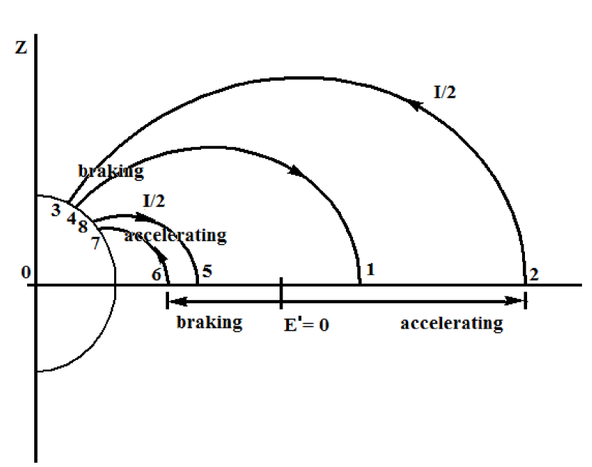
Figure 1: This figure illustrates the unipolar electric field interaction scheme. The position $\vec{E}^{\prime}=0$ indicates the null of the electric field in the rotating frame of the disk plasma, from which the current of the resistive disk flows inward towards the star and outward away from the star. The inner current loop is completed through the equipotential field lines to the stellar surface and back (5-6-7-8-5), likewise is the outer loop (1-2-3-4-1). Through these current loops, torque and counter torque are applied on the disk and star respectively, and vice verse, and corresponding strong toroidal magnetic fields can also be generated.

where $\vec{E}^{{}^{\prime}}$ is the electric field in the disk rotating frame, $\vec{v}_{D}$ and $\Omega_{D}$ are the Kepler linear velocity and angular velocity of the disk, and $\nabla\Psi$ is pointing inward towards the star. We note that this equation is not the Ohm law with resistivity in the MHD system of the magnetosphere. It is the Ohm law of the disk plasma under an external magnetic field. For $r<r_{co}$, the disk current flows inward generating a braking torque on the disk, while for $r_{co}<r$, the disk current flows outward exerting an accelerating torque. Because of this current flow on the disk, toroidal magnetic fields with opposite signs are immediately generated on both sides of the equatorial disk plane. Since $\nabla\cdot\vec{J}=0$, there are return currents along the disk. For the inner disk, these currents follow the equipotential magnetic field lines to the mid latitudes of the star and return back to the disk before $r_{co}$, generating a counter (accelerating) torque on the star. Likewise is the return currents of the outer disk which generate a counter (braking) torque at the high latitude polar region. Half of the disk current returns from the northern hemisphere, and the other half returns from the southern part. In the presence of the toroidal field, the field line twists around the toroidal direction as it follows through the poloidal direction, and Fig.(1) represents the projection of the twisting field line on the poloidal plane.

Here, by magnetosphere, we mean the overall closed stellar magnetic field lines even those intercepting the disk on the equatorial plane, not just the closed field lines inside the disk inner boundary $r_{m}$. Although we have assumed equipotential field lines such that the unipolar field $\vec{E}_{*}$ could be projected onto the disk, this projection is not effective at large distances either because the magnetospheric plasma density is not dense enough to ensure perfect conductivity and high plasma mobility, or the magnetic field is too weak to warrant a MHD state. Only as the disk accrets closer to the star that the unipolar field projection becomes effective. In the rotating field line paradigm, the toroidal field is generated by the differential rotation between the disk plasma and the rotating field lines. However, there is no clarification of the axial current to account for the toroidal field. The toroidal field generation is treated as a magnetostatic problem (van Ballegooijin, 1994; Lovelace et al., 1995; Lynden-Bell, 1996).

In the present unipolar model, the star-disk current loops become a site of generating additional magnetic fields, both toroidal and poloidal, driven by the rotational energy of the star. The toroidal fields in the northern and southern hemispheres have different signs, which require a self-consistent disk current sheet as the boundary condition on the equatorial plane. Integrating the Ampere law over the contour of a cross section of the disk transverse to a given radial direction, we get

$$\vec{B}_{\phi north}\cdot\hat{l}_{north}+\vec{B}_{\phi south}\cdot\hat{l}_{south}\,=\,\mu_{0}J_{r}\Delta z\,=\,\mu_{0}\sigma A_{0}(\Omega_{D}-\Omega_{*}){\partial\Psi\over\partial r}\Delta z\,\,\,,$$ (8)

where $\Delta z$ is the thickness of the disk, $\hat{l}_{north}$ is the unit vector of the toroidal field in the northern hemisphere, likewise is $\hat{l}_{south}$. Considering the disk be located outside the corotation radius $r_{co}$, the disk current is in the $+\hat{r}$ direction, the toroidal field in the northern hemisphere is in the $-\hat{\phi}$ direction with $A_{\phi}=-A_{\phi abs}$ where $A_{\phi abs}$ is the absolute value of the magnetic flux. In the southern side, we have $A_{\phi}=+A_{\phi abs}$. The boundary condition of the disk current sheet is, therefore,

$$2A_{\phi abs}A(\Psi){1\over r}\,=\,-\mu_{0}\sigma(r)A_{0}(\Omega_{*}-\Omega_{D}(r)){\partial\Psi\over\partial r}\Delta z\,\,\,.$$ (9)

4 Nonlinear Force-Free Magnetosphere

Over the evolution history of a magnetic star, we assume that a force-free magnetosphere of quasi-neutral plasma with the corresponding self-consistent current density is formed, described by

$$\vec{J}\times\vec{B}=0\,\,\,.$$ (10)

The toroidal and poloidal components of this force-free field equation render

$$A\,=\,A(\Psi)\,\,\,,$$ (11)

$${\partial^{2}\Psi\over\partial r^{2}}+{1\over r^{2}}\sin\theta{\partial\over\partial\theta}\left({1\over\sin\theta}{\partial\Psi\over\partial\theta}\right)+\alpha^{2}A(\Psi){\partial A(\Psi)\over\partial\Psi}\,=\,0\,\,\,.$$ (12)

To solve the force-free field, we have to specify the source function $A(\Psi)$. Should we take a linear dependence for $A(\psi)=a_{0}\Psi$, we would get the well known linear force-free field solution. We prefer to view the magnetosphere as a magnetically stressed system and seek a nonlinear description to represent it. We thus follow Lynden-Bell & Boily (1994) to consider the coefficient as a function of $\Psi$ itself to write

$$A(\Psi)\,=\,a_{0}\Psi^{1/n}\Psi\,=\,a_{0}\Psi^{1+1/n}\,\,\,,$$ (13)

where $a_{0}$ has the dimension of an inverse scale length and $n$ is the similarity parameter, and get

$$r^{2}{\partial^{2}\Psi\over\partial r^{2}}+\sin\theta{\partial\over\partial\theta}\left({1\over\sin\theta}{\partial\Psi\over\partial\theta}\right)+\left(1+{1\over n}\right)\alpha^{2}a^{2}_{0}r^{2}\Psi^{1+2/n}\,=\,0\,\,\,.$$ (14)

Separating the variables by writing $\Psi(r,\theta)=R(r)\Theta(\theta)$ gives

$${1\over R}r^{2}{\partial^{2}R\over\partial r^{2}}\,=\,-\left[{1\over\Theta}\sin\theta{\partial\over\partial\theta}\left({1\over\sin\theta}{\partial\Theta\over\partial\theta}\right)+\left(1+{1\over n}\right)\alpha^{2}a^{2}_{0}r^{2}R^{+2/n}\Theta^{+2/n}\right]\,=\,n^{\prime}(n^{\prime}+1)\,\,\,,$$ (15)

where $n^{\prime}$ is the separation constant. In terms of the normalized radial distance $\xi=r/r_{0}$ where $r_{0}$ is the radius of the magnetic star, the radial function $R(\xi)$ is given by

$$\xi^{2}{\partial^{2}R\over\partial\xi^{2}}\,=\,n^{\prime}(n^{\prime}+1)R\,\,\,,$$ (16)

$$R(\xi)\,=\,\xi^{n^{\prime}+1}\,\,\,,\,\,\,\,\,\,\xi^{-n^{\prime}}\,\,\,.$$ (17)

As for the meridian function $\Theta(\theta)$, we have

$$\sin\theta{\partial\over\partial\theta}\left({1\over\sin\theta}{\partial\Theta\over\partial\theta}\right)+n^{\prime}(n^{\prime}+1)\Theta\,=\,-{(n+1)\over n}(\alpha a_{0}r_{0})^{2}\xi^{2}R^{+2/n}\Theta^{1+2/n}\,\,\,.$$ (18)

With $R(\xi)=\xi^{-n^{\prime}}$, we get the mode equation that reads

$$(1-x^{2}){d^{2}\Theta(x)\over dx^{2}}+n^{\prime}(n^{\prime}+1)\Theta(x)\,=\,-{(n^{\prime}+1)\over n^{\prime}}(\alpha a_{0}r_{0})^{2}\Theta^{1+2/n^{\prime}}(x)\,\,\,,$$ (19)

where $x=\cos\theta$ and we have taken $n^{\prime}=n$. From the field line equation, the twist angle of the field line in space $\phi(x)$ and the corresponding toroidal magnetic field are governed by

$$d\phi(x)\,=\,-(\alpha a_{0}r_{0}){1\over n^{\prime}}{1\over(1-x^{2})}\Theta^{1/n^{\prime}}(x)dx\,\,\,,$$ (20)

$$B_{\phi}\,=\,{A_{0}\over r_{0}^{2}}(\alpha a_{0}r_{0}){1\over\xi\sin\theta}\Psi^{1+1/n^{\prime}}\,\,\,.$$ (21)

Once $\Theta(x)$ is solved from the mode equation, the twist angle $\phi(x)$ can be integrated to get its profile in space.

5 Stressed Magnetosphere

With the right side of Eq.(19) null for $\alpha=0$ or $A_{\phi}=0$, the linear solution is

$$\Theta(x)\,=\,(1-x^{2}){dP_{n^{\prime}}(x)\over dx}\,\,\,,$$ (22)

with integer $n^{\prime}=1,2,3,...$ where $P_{n^{\prime}}(x)$ is the Legendre polynomial. With $n^{\prime}=n=1$, the poloidal field lines are given by

$$\Psi(\xi,\theta)\,=\,R(\xi)\Theta(x)\,=\,{\sin^{2}\theta\over\xi}\,=\,C\,\,\,,$$ (23)

which corresponds to the dipole field. For $\alpha\neq 0$, the meridian function $\Theta(x)$ is stressed through the right side of Eq.(19) generating a nonlinear $\Theta(x)$ with $n^{\prime}$ deviating from integers. To represent the magnetospheric field as an external field, not anchored on and twisted by the disk plasma, we take the boundary condition of $\Theta(x)$ on the disk at $x=0$ as

$${d\Theta(x)\over dx}\,=\,0\,\,\,,$$ (24)

in order to assure the poloidal field line be normal to the conducting disk. Solving for the mode equation with $R(\xi)=\xi^{-n^{\prime}}$ and with $n^{\prime}=n$, the response of the eigenvalue $\alpha a_{0}r_{0}$ to the separation constant $n^{\prime}$ is shown in Fig.2. The separation constant $n^{\prime}$ begins from $n^{\prime}=1$ for $\alpha a_{0}r_{0}=0$, and as $n^{\prime}$ decreases the eigenvalue increases. However, as the separation constant goes beyond $n^{\prime}=0.720$, there is no eigenvalue $\alpha a_{0}r_{0}$ to allow an eigenfunction $\Theta(x)$. In this sense, $n^{\prime}=0.720$ is the stress limit of the nonlinear description of $\Theta(x)$. The stressed eigenfunctions $\Theta(x)$ whose nonlinearity changes with $n^{\prime}$ are shown in Fig.3. Three values of $n^{\prime}=0.998,0.853,0.720$ are chosen corresponding to $\alpha a_{0}r_{0}=0.10,0.50,0.59$ respectively. Furthermore, the poloidal field line contours with $C=0.2$ are plotted in Fig.4. The contour $C=0$ is the polar axis. With $C=0.2$, the field lines of Fig.4 are originated in the polar region, and they are the stressed counterpart of the linear dipole field lines. As the contour value $C$ increases, the poloidal field lines will come from a region of lower latitude of the star and will reach the inner part of the disk closer to the star. The plasma disk, which is not shown in this figure, lies on the equatorial plane extending from $\xi>\xi_{co}$ outward. The twist angles in space $\phi(x)$ are illustrated in Fig.5, and the dimensionless toroidal fields $B_{\phi}(x)$, without the dimensional $A_{0}/r_{0}^{2}$ factor, at a given radius $\xi=5$ on the disk plane at $x=0$ are illustrated in Fig.6. In Fig.5, the twist angle in space increases with the eigenvalue, in particular on the disk plane. In Fig.6, the toroidal field on the disk increases with the eigenvalue, thus with the twist angle. Within this stressed magnetosphere model, the field line twisting reaches its limit as $n=n^{\prime}=0.720$ corresponding to $\alpha a_{0}r_{0}=0.59$. The toroidal magnetic field saturates at this limit. The dimensionless toroidal fields $B_{\phi}(x)$, without the dimensional $A_{0}/r_{0}^{2}$ factor, along the trajectories of three poloidal field lines are indicated in Fig.7. As a result, Fig.4 and Fig.7 together show spiralling magnetospheric field lines down to the star.

6 Angular Momentum Extraction

Let us now examine the current sheet boundary condition on the equatorial plane. First of all, the circumference of the disk increases as $r$, and to maintain a current flow on the disk, the plasma conductivity has to scale as $1/r$ by axisymmetry. In terms of the normalized radial distance $\xi$, $\sigma(r)=\kappa/r=\kappa/(r_{0}\xi)$. Furthermore, we consider the inner disk boundary be located at a fair distance beyond $\xi_{co}$ such that $(\Omega_{*}-\Omega_{D}(\xi))$ can be regarded as insensitive to $\xi$. This point can also be supported by the accelerating torque on the disk which reduces the angular velocity gradient across the disk. With these considerations, and using Eq.(13) and $R(\xi)=\xi^{-n^{\prime}}$, the $\xi$ dependence has canceled out from both sides of the boundary condition, Eq.(9), leaving only

$$2A_{\phi abs}a_{0}r_{0}\Theta^{1/n}(x)\,=\,\mu_{0}\kappa A_{0}n(\Omega_{*}-\Omega_{D})\Delta z\,\,\,.$$ (25)

This condition contains the disk parameters $\sigma,\Omega_{D},\Delta z$, the field parameters $A_{\phi abs},A_{0},a_{0}$, and the meridian function $\Theta(x)$ evaluated at $x=0$. As the field parameters evolve over time, the disk parameters have to evolve accordingly. To bind the opposing extraordinary toroidal fields together, the disk should carry an ultra high current density which would certainly heat up the disk to extreme temperatures. This enhances the degree of ionization of the disk plasma which allows the disk to carry more current. Furthermore, the corresponding blackbody radiations of the disk temperature might be related to quiescent X-ray emissions. As the toroidal field in the magnetosphere builds up, the magnetic pressure compresses the disk increasing its density, thus further enhancing the plasma conductivity and allowing the disk to carry even more current. The compression of the disk by the magnetic pressure counteracts the propeller effect caused by the accelerating torque on the disk and keeps the disk on the equatorial plane. Under this scenario, we can therefore regard the magnetosphere as a site where the rotational energy of the star is stored in the form of magnetic energy through the toroidal and poloidal fields via the unipolar induction.

By uploading the potential distribution on the stellar surface to the equipotential field lines of the magnetosphere, the unipolar stellar electric field $\vec{E}_{*}$, generated by the angular momentum of the star, is transferred to the magnetosphere. Consequently, there is an electromagnetic momentum in the magnetosphere given by the Poynting vector

$$\mu_{0}\vec{S}\,=\,\vec{E}_{*}\times\vec{B}\,=\,V_{*}A_{0}(\nabla\Psi\cdot\nabla\Psi)\nabla\phi\mp V_{*}A_{\phi abs}A\nabla\Psi\times\nabla\phi\,\,\,.$$ (26)

The first term is the toroidal momentum whereas the second term is the poloidal momentum with the upper/lower sign for the southern/northern hemisphere. Summing over the entire magnetosphere, the southern and the northern poloidal momentum cancel each other, leaving only the toroidal momentum. The corresponding electromagnetic angular momentum with respect to the center of the star is $\vec{L}=\vec{r}\times\vec{S}$. This angular momentum has a toroidal part and a poloidal part. Summing over the entire magnetosphere, it is clear that the toroidal part vanishes while the poloidal part adds up to a z component along the polar axis as is the angular momentum of the star. Most of the time, we often think of electromagnetic fields as fields only. But the momentum and angular momentum associated to the electromagnetic fields are just as real and physical as the mechanical counterparts. These electromagnetic momentum and angular momentum in the stationary magnetosphere can further be coupled to the magnetospheric plasma through the $\vec{E}\times\vec{B}$ drift, as if it were dragged by the rotating field lines. We therefore have a star-magnetosphere system where angular momentum of the star can be coupled to the magnetosphere and further to the plasma there. On the other hand, the star losses angular momentum due to the unipolar current flow in the interior of the star, which exercises a braking torque on the star. This star-magnetosphere system underlines the conservative nature of the total angular momentum, mechanical and electromagnetic.

We remark that in this model the star-disk system acts like an astrophysical power circuit where the star is the generator and the disk is the external load. Through the current flows between the star and the disk, the toroidal and poloidal force-free magnetic fields are enhanced in the northern and southern hemispheres. This provides a site where extraordinary toroidal fields are generated at the expense of the stellar rotational energy. The toroidal flux stored in the magnetosphere is directly related to the current carrying capacity of the disk, which is a function of the plasma conductivity. As the magnetic flux keeps increasing, it eventually exceeds the current carrying limit of the disk, generating a violent magnetic eruption and sending Poynting fluxes into space either isotropically or beamed. With the electromagnetic angular momentum being extracted, it leaves the star to establish anew its magnetosphere with the disk as a plasma source to refill the nearby stellar space through diffusion.

7 Conclusions

We have pointed out in the current rotating field line model of star-disk interaction two basic problems. First, magnetic field line, like velocity stream line, is a concept devised to help visualize the actions of the magnetic field. Magnetic field line is not a real physical variable and it cannot take actions to drag plasmas to corotate. This generates an internal inconsistency in this rotating field line model where the rotation induced electric field should be zero because there is no relative velocity between the rotating plasma and the rotating field. However, the rotation induced electric field has always been calculated as if the magnetic field were stationary in space. Second, the disk is a gravitational system and it does not form an ideal MHD system with the stellar magnetosphere. The two systems are not described under the same set of MHD equations. Consequently, the frozen-field theorem cannot be applied. We have, therefore, proposed a unipolar induction star-disk interaction model with stationary magnetic fields in space where the unipolar stellar electric field is uploaded to the magnetosphere generating a star-magnetosphere coupled system with angular momentum conservation, the mechanical one of the star and the electromagnetic one of the magnetosphere. The electromagnetic one of the magnetosphere can further be coupled to the plasma there through the $\vec{E}\times\vec{B}$ drift, as if the plasma were dragged by the rotating field lines. In this model, the interaction between the star and the disk is through the projection of the uploaded stellar electric field onto the disk, thus generating a current flow on the disk with return current loops via the stellar surface, forming a site where intense toroidal and poloidal magnetic fields can be generated from the rotational energy of the star. The opposing toroidal magnetic fields in the northern and southern hemispheres are held together by the disk current sheet under the self-consistent boundary condition, which is a function of the disk parameters. Angular momentum of this star-disk system can be extracted when the magnetic flux in the magnetosphere grows so much that it exceeds the current carrying capacity of the disk leading to the repulsion of the mega toroidal fields and sending Poynting fluxes into space.

Figure 2: The eigenvalue $\alpha a_{0}r_{0}$ of the mode equation is shown as a function of the separation constant $n^{\prime}$.

Figure 3: The stressed eigenfunctions $\Theta(x)$ are shown in a polar plot for $\alpha a_{0}r_{0}=0.10,0.50,0.59$ corresponding to $n^{\prime}=0.998,0.853,0.720$ respectively for the three plots from left to right.

Figure 4: The poloidal field lines $\Psi(\xi,x)=C$ with $C=0.20$ are shown in a cartesian $(\rho,z)$ plot, where $\rho=\xi\sin\theta$, in units of normalized distance $\xi$ for the three eigenfunctions $\Theta(x)$ of Fig.2 from left to right. The contour of $C=0$ is the polar axis. As the contour value $C$ increases, the contours move closer to the equatorial plane and to the star.

Figure 5: The twist angles $\phi(\theta)$ in space are plotted against the polar angle $\theta$ for the three field lines $\Psi(\xi,x)=C=0.20$ with $\alpha a_{0}r_{0}=0.10,0.50,0.59$ for the lower, middle, upper curves respectively.

Figure 6: The dimensionless toroidal magnetic fields $B_{\phi}$ on the disk plane at $\xi=5$ are plotted against the eigenvalues $\alpha a_{0}r_{0}$.

Figure 7: The dimensionless toroidal magnetic fields $B_{\phi}$ are plotted along the three poloidal field lines.

References

- Bardou & Heyvaerts (1996) Bardou, A. & Heyvaerts, J., 1996. Interaction of a stellar magnetic field with a turbulent accretion disk, A&A, 307, 1009-1022.
- Blandford (1976) Blandford, R.D., 1976. Accretion disc electrodynamics - A model for double radio sources, MNRAS, 176, 465-481.
- Blandford & Payne (1982) Blandford, R.D. & Payne, D.G., 1982. Hydromagnetic flows from accretion discs and the production of radio jets, MNRAS, 199, 883-903.
- Bogovalov (1996) Bogovalov, S.V., 1996. Plasma flow in the magnetosphere of an axisymmetric rotator, MNRAS, 280, 39-52.
- Bogovalov & Tsinganos (1999) Bogovalov, S.V. & Tsinganos, K., 1999. On the magnetic acceleration and collimation of astrophysical outflows, MNRAS, 385, 211-224.
- Cao & Spruit (1994) Cao, X. & Spruit, H.C., 1994. Magnetically driven wind from an accretion disk with low-inclination field lines, A&A, 287, 80-86.
- Henriksen & Rayburn (1971) Henriksen, R.N. & Rayburn, D.R., 1971. Relativistic stellar wind theory : Near zone solutions, MNRAS, 152, 323-332.
- Illarionov & Sunyaev (1975) Illarionov, A.F. & Sunyaev, R.A., 1975. Why the number of Galactic X-ray stars is so small?, A&A, 39, 185-195.
- Jackson (1975) Jackson, J.D., 1975. Classical Electrodynamics, Chapter 12, John Wiley & Sons, New York.
- Lovelace et al. (1986) Lovelace, R.V.E., Mehanian, C., Mobarry, C.M., & Sulkanen, M.E., 1986. Theory of axisymmetric magnetohydrodynamic flows : Disks, ApJS, 62, 1-37.
- Lovelace et al. (1995) Lovelace, R.V.E., Romanova, M.M., & Bisnovatyi-Kogan, G.S., 1995. Spin-up/spin-down of magnetized stars with accretion discs and outflows, MNRAS, 275, 244-254.
- Lynden-Bell (1996) Lynden-Bell, D., 1996. Magnetic collimation by accretion discs of qusars and stars, MNRAS, 279, 389-401.
- Lynden-Bell & Boily (1994) Lynden-Bell, D. & Boily, C., 1994. Self-similar solutions up to flashpoint in highly wound magnetostatics, MNRAS, 267, 146-152.
- Mestel (1968) Mestel, L., 1968. Magnetic braking by a stellar wind - I, MNRAS, 138, 359-391.
- Romanova et al. (2003) Romanova, M.M., Toropina, O.D., Toropin, Y.M., & Lovelace, R.V.E., 2003. Magnetohydrodynamic simulations of accretion onto a star in the ’Propeller’ regime, ApJ, 588, 400-407.
- Schmidt (1966) Schmidt, G., 1966. Physics of High Temperature Plasmas, Chapter II, Academic Press, New York.
- Tsinganos & Bogovalov (2000) Tsinganos, K. & Bogovalov, S.V., 2000. Magnetic collimation of the solar and stellar winds, A&A, 356, 989-1002.
- Tsui (2015) Tsui, K.H., 2015. The pulsating pulsar magnetosphere, ApJ, 805, 106.
- Thompson (1962) Thompson, W.B., 1962. An Introduction to Plasma Physics, Chapter 7, Addison-Wesley, London.
- Ustyngova et al. (2006) Ustyngova, G.V., Koldoba, A.V., Romanova, M.M., & Lovelace, R.V.E., 2006. ’Propeller’ regime of disk accretion to rapidly rotating stars, ApJ, 646, 304-318.
- van Ballegooijin (1994) van Ballegooijen, A.A., 1994. Energy release in stellar magnetospheres, Space Science Reviews, 68, 299-307.