Cover time for random walks on arbitrary complex networks

Abstract

We present an analytical method for computing the mean cover time of a discrete time random walk process on arbitrary, complex networks. The cover time is defined as the time a random walker requires to visit every node in the network at least once. This quantity is particularly important for random search processes and target localization on network structures. Based on the global mean first passage time of target nodes we derive a method for computing the cumulative distribution function of the cover time based on first passage time statistics. Our method is viable for networks on which random walks equilibrate quickly. We show that it can be applied successfully to various model and real-world networks. Our results reveal an intimate link between first passage and cover time statistics and offer a computationally efficient way for estimating cover times in network related applications.

I Introduction

Random walks have been studied extensively for more than a century and emerged as an efficient descriptive model for spreading and diffusion processes in physics, biology, social sciences, epidemiology, and computer science oksendal_stochastic_1992 ; berg_random_1993 ; barrat_dynamical_2008 ; Brockmann:2008hb ; newman_networks:_2010 ; klafter_first_2011 ; masuda_random_2016 . Because of their wide applicability and relevance to dynamic phenomena, random walk processes have become a topic of interest particularly for analyses of dynamics on complex networks masuda_random_2016 . The calculation of a resistor network’s total resistance newman_networks:_2010 , synchronization phenomena in networks of coupled oscillators barrat_dynamical_2008 , the global spread of infectious diseases on the global air traffic network Hufnagel:2004kta ; Brockmann:2013ud ; iannelli_effective_2017 and ranking the importance of single websites in the world wide web page_pagerank_1999 are just a few examples of systems that have been investigated based on concepts derived from random walk theory.

Especially important is the understanding of temporal aspects of stochastic processes and how different network structures influence the equilibration process. Consequently, a lot of theoretical work focused on understanding the connection between network structure and relaxation time scales or first passage times (FPTs), the time it takes a single walker to travel from one node to another. Both, relaxation and first passage times quantify different aspects but fail to capture the characteristic time a walker requires on average to visit every node in a network, which is captured by the cover time of the process. This quantity, however, has important practical applications from biology to computer science, for instance, for estimating how long it will take to distribute a chemical or a certain commodity to every node in a network or as a measure for navigability in multilayer transportation networks domenico_navigability_2014 . Researchers have been able to derive analytically asymptotic results for the cover time for some model networks, e.g. complete graphs, Erdős–Rényi (ER) and Barabási–Albert (BA) networks cooper_cover_2007 ; cooper_cover_2007-1 ; lovasz_random_1996 . Yet, only few analytical or heuristic results concerning the mean cover time of real-world networks have been established, it is thus unclear how a real-world network’s mean cover time is related to other temporal features of random walks on these networks and how their structure and topological features may impact cover time statistics.

In the following, we present a theoretical approach that predicts the cover time on arbitrary complex networks using only FPT statistics. We show that for networks on which random walks equilibrate quickly (specified below), the cover time can be estimated accurately by the maximum of a set of FPTs drawn from the ensemble of FPT distributions of all target nodes. Our method’s predictions are in excellent agreement with results provided by computer simulations for a variety of real-world networks, as well as for ER networks, BA networks, complete graphs and random $k$-regular networks. We also show that our method fails when the conditions of rapid relaxation are violated, e.g. for networks embedded in a low-dimensional space with short-range connection probability.

II Theory

II.1 Random walks and first passage times

The foundation of our analysis is an unweighted, undirected, network composed of $N$ nodes, $E$ links and adjacency matrix $A_{vu}$ with $A_{vu}=1$ if node $u$ and $v$ are connected and $A_{vu}=0$ if not. On this network, we consider a simple discrete time random walk that starts on an initial node $u$ at time $t=0$. At every time step, the walker jumps randomly to an adjacent node $v$. The process is repeated indefinitely and is goverened by the master equation

$$P_{v}(t+1)=\sum_{u=1}^{N}W_{vu}P_{u}(t),$$

where $P_{u}(t)$ is the probability that the walker is at node $u$ at time $t$, $W_{vu}=A_{vu}/k_{u}$ is the transition probability of the walker going from node $u$ to node $v$ in one time step, and $k_{u}=\sum_{v=1}^{N}A_{vu}$ is the degree of node $u$. We assume that the network has a single component, so every node can be reached, in principle, from every other node. Generally, this process will approach the equilibrium $P_{v}^{\star}=k_{v}/2E.$

Central questions for random walks are often connected to first passage times (FPT), e.g. the mean first passage time $\tau_{vu}$ (MFPT) between two nodes $u$ and $v$. This time is defined as the mean number of steps it takes a random walker starting at node $u$ to first arrive at node $v$. Another important quantity is the global mean first passage time of node $v$ (GMFPT), obtained by averaging the MFPT over all possible starting nodes:

$$\tau_{v}=\frac{1}{N-1}\sum_{u\neq v}\tau_{vu}.$$ (1)

The GMFPT can be used as a measure of centrality for node $v$ since a node that is quickly reachable from anywhere may be interpreted to be “important”. Passage times have been well analyzed and can be computed efficiently from network properties. Given the unnormalized graph Laplacian

$$L_{vu}=k_{v}\delta_{vu}-A_{vu},$$

where $\delta_{vu}$ denotes Kronecker’s delta, the MFPT between two nodes can be computed by spectral decomposition newman_networks:_2010 ; lin_mean_2012 . Given the operator’s eigenvalues $0=\lambda_{1}<\lambda_{2}\leq...\leq\lambda_{N}$ and corresponding orthonormal eigenvectors $\mu_{i}=(\mu_{i1},\mu_{i2},...,\mu_{iN})^{T}$, one can compute node $v$’s exact GMFPT as

$$\tau_{v}^{\mathrm{ex}}=\frac{N}{N-1}\sum_{i=2}^{N}\frac{1}{\lambda_{i}}\left(2E\mu_{iv}^{2}-\mu_{iv}\sum_{n}k_{n}\mu_{in}\right).$$ (2)

A computationally more efficient method estimates the GMFPT by its lower bound, which is given by

$$\tau_{v}^{\mathrm{es}}\geq\frac{N\left\langle k\right\rangle}{k_{v}}\frac{1}{1-\left\langle k\right\rangle^{-1}},$$ (3)

if the process equilibrates quickly, i.e. when the relaxation time fullfills $t_{\mathrm{rlx}}\ll N$, which holds within small relative errors for Erdős–Rényi (ER) and Barabási–Albert (BA) networks, as well as for a variety of real-world networks lau_asymptotic_2010 . The relaxation time of a random walk on a network can be bounded from below using the second smallest eigenvalue $\lambda_{2}$ of $L_{vu}$ mohar_applications_1997 as

$$t_{\mathrm{rlx}}\geq\lambda_{2}^{-1}.$$ (4)

Another temporal characteristic with practical relevance is the mean cover time $T_{u}$, defined as the mean number of steps it takes a random walker starting at node $u$ to visit every other node at least once. For various network models simple heuristics concerning the asymptotic scaling of the mean cover time as a function of network size $N$ have been derived cooper_cover_2007 ; cooper_cover_2007-1 ; lovasz_random_1996 . For ER, BA and fully connected networks it was shown that

$$\left\langle T\right\rangle\sim\alpha\,N\log N,$$

with network specific prefactor $\alpha$. Here, $A_{N}\sim B_{N}$ means $\lim_{N\rightarrow\infty}A_{N}/B_{N}=1$ as in Ref. cooper_cover_2007-1 . Such scaling relationships are useful for comparative analyses, e.g. when networks for different sizes of the same class are compared. They are less helpful when actual expected cover times need to be computed for empirical networks where $N$ is fixed and comparative or relative statements are insufficient.

Unfortunately, a general procedure for estimating the actual cover time for arbitrary complex networks, as well as the connection between the mean cover time and FPT observables is lacking. In the following we present a method that estimates the cover time using passage time statistics.

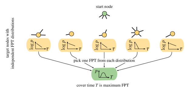
Figure 1: Illustration of our approach. Each node of the network is viewed as an independent entity that can be visited by the walker starting at the green node. Each target node $v$ has its own first passage time (FPT) distribution which is asymptotically (for larger times $\tau$) distributed as $\propto\exp(-\tau/\tau_{v})$ with its global mean FPT $\tau_{v}$. In order to compute the cover time, we draw one FPT $\tau$ from every target’s distribution. Then the cover time is given as the maximum time of all drawn FPTs.

II.2 Cover Time

Recently it has been found that if a random walk process equilibrates quickly, i.e. the initial concentration of random walkers approaches the equilibrium concentration in a small number of time steps $t_{\mathrm{rlx}}\ll N$, the information about the start node is lost lau_asymptotic_2010 and the first passage time at destination $v$ is (for larger times $\tau$) distributed asymptotically according to

$$p_{v}(\tau)\propto\exp(-\tau/\tau_{v})$$

where $\tau_{v}$ is the GMFPT of Eq. (1). $\tau_{v}$ can differ between nodes and depends on the topological features of the network only. Note that in the following paragraphs we will often refer to the FPT decay rate $\beta_{v}=\tau_{v}^{-1}$ instead of the GMFPT, simplifying the notation.

In order to find the mean cover time from the collection of distributions $p_{v}(\tau)$ we proceed as illustrated in Fig. 1. Excluding the start node $u$, we pick an FPT $t_{v}$ for each target node $v$ from their respective FPT distribution $p_{v}$ at random, resulting in a set of $N-1$ FPT that we call $\mathcal{F}$. Consequently, the cover time $T_{u}$ is given as the maximum element of $\mathcal{F}$. In order to find the distribution of this maximum, we compute the probability that a time $T$ is an upper bound of this set as the probability that no element of $\mathcal{F}$ is larger than $T$, yielding

$$P_{u}(T) = P_{u}(\mathrm{``}T\ \mathrm{is}\ \mathrm{an\ upper\ bound\ of\ FPTs"})$$ (5)

$$= P_{u}(t_{v}\leq T\ \forall t_{v}\in\mathcal{F})=\prod_{v\neq u}P_{u}(t_{v}\leq T).$$

We further approximate our result by assuming a continuous time distribution, easing the computations without significantly changing the outcome as explained in App. B. Then, the probability that any time $t_{v}\in\mathcal{F}$ is lower than or equal to $T$ is

$$P(t_{v}\leq T) =\int\limits_{0}^{T}\mathrm{d}t\ p_{v}(t)=\int\limits_{0}^{T}\mathrm{d}t\ \beta_{v}\exp(-\beta_{v}t)$$

$$=1-\exp(-\beta_{v}T).$$ (6)

Eqs. (5) and (6) yield the cumulative distribution function for the cover time,

$$P_{u}(T)=\prod_{v\neq u}\Big{(}1-\exp(-\beta_{v}T)\Big{)}$$

and the expected cover time

$$T_{u} \approx\int\limits_{0}^{\infty}\mathrm{d}T\ \left[1-\prod_{v\neq u}\left(1-\exp(-\beta_{v}T)\right)\right]-\frac{1}{2}.$$ (7)

As discussed in App. B, the additional shift of $1/2$ emerges when changing from discrete time to continuous time. However, since the mean cover time is usually $T_{u}\gg 1/2$, we will omit this shift, introducing relative error of $(2T_{u})^{-1}.$ We can find the global mean cover time by averaging over target nodes $u$ as

$$\left\langle T\right\rangle \approx\int\limits_{0}^{\infty}\mathrm{d}T\left[1-P(T)\frac{1}{N}\sum_{u=1}^{N}\frac{1}{1-\exp(-\beta_{u}T)}\right]$$ (8)

with

$$P(T)=\prod_{v=1}^{N}\left(1-\exp(-\beta_{v}T)\right).$$ (9)

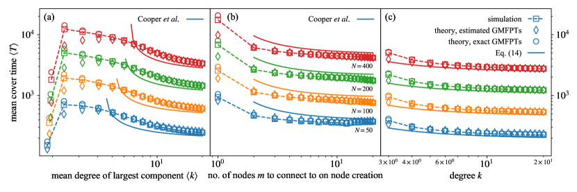
Figure 2: The mean cover time $\left\langle T\right\rangle$ of the largest component of (a) Erdős–Rényi (ER) networks, (b) Barabási–Albert (BA) networks , and (c) random $k$-regular networks. Shown are averages measured from 1000 simulations per data point ($\boxempty$) and both estimations of the mean cover time using ($\diamondsuit$) estimated GMFPTs from the target nodes’ degrees Eq. (11) and ($\varbigcirc$) exact GMFPTs Eq. (12) computed from the unnormalized graph Laplacian’s spectrum in (a) and (b). Respectively, we used Eq. (13) for random $k$-regular networks in (c). Dashed lines are simulation results and a guide to the eye. Further displayed are the asymptotic results derived by Cooper, et. al. for the ER cooper_cover_2007 and BA cooper_cover_2007-1 network model as well as the lower bound Eq. (14) for random $k$-regular networks.

However, as shown in App. C, introducing small relative error of order $\mathcal{O}\left((N\log N)^{-1}\right)$ for the networks discussed in this paper, we will make use of a simpler integral to find

$$\left\langle T\right\rangle \approx\int\limits_{0}^{\infty}\mathrm{d}T\left[1-P(T)\right]=\int\limits_{0}^{\infty}\mathrm{d}T\left[1-\prod_{v=1}^{N}\left(1-\exp(-\beta_{v}T)\right)\right]$$ (10)

$$=\sum_{\mathcal{S}\in\mathcal{P}^{*}(\mathcal{V})}(-1)^{|\mathcal{S}|+1}\left(\sum_{v\in\mathcal{S}}\beta_{v}\right)^{-1}.$$

Here, $\mathcal{V}$ is the set of all nodes and $\mathcal{P}^{*}(\mathcal{V})$ is the set of all possible subsets of $\mathcal{V}$ excluding the empty set. Conceptually, this integral equals a situation where an additional node is inserted on which every random walk starts but which can never be visited again. Even though one can solve integral Eq. (10) analytically to obtain the result above, in practice it is more feasible to solve the integral numerically than iterating over $\mathcal{P}^{*}(\mathcal{V})$ which has $2^{N}-1$ elements and hence becomes very large rather quickly.

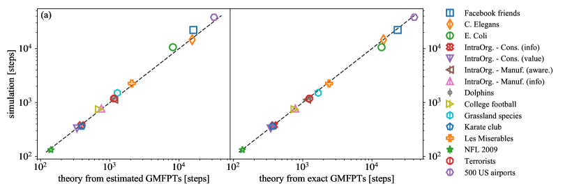
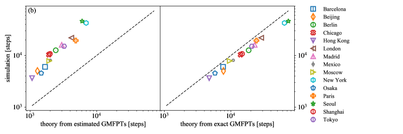
Figure 3: Mean cover times of simple discrete time random walks on the largest component of (a) various real-world networks (data sources and relative errors given in Tab. 1) and (b) various subway networks (data source and relative errors given in Tab. 2). The estimated cover times are compared to the measured cover times (from 50 simulations for each data point). The dashed lines represent the ideal case $\left\langle T^{\mathrm{sim}}\right\rangle=\left\langle T^{\mathrm{es/ex}}\right\rangle$. Theoretical results are computed from (left) estimated GMFPTs from the target nodes’ degrees Eq. (11) and (right) exact GMFPTs computed from the unnormalized graph Laplacian’s spectrum Eq. (12).

Now, the estimation of the global mean cover time reduces to an efficient estimation of the FPT decay rates $\beta_{v}$. There are two ways to estimate the decay rates with the GMFPTs as described in Sec. II.1. Using the estimation of the lower bound Eq. (3), the estimated global mean cover time is given by

$$\left\langle T^{\mathrm{es}}\right\rangle\geq\int\limits_{0}^{\infty}\mathrm{d}T\left[1-\prod_{v=1}^{N}\left(1-\exp\left(-Tk_{v}\frac{1-\left\langle k\right\rangle^{-1}}{N\left\langle k\right\rangle}\right)\right)\right].$$ (11)

The advantage of this method is that only the network’s degree sequence $k_{v}$ needs to be known in order to estimate the global mean cover time. However, this method can obviously only account for a lower bound. We can also compute the exact GMFPTs using Eq. (2). In this case the computed global mean cover time is

$$\left\langle T^{\mathrm{ex}}\right\rangle=\int\limits_{0}^{\infty}\mathrm{d}T\left[1-\prod_{v=1}^{N}\left(1-\exp\left(-\frac{T}{\tau_{v}^{\mathrm{ex}}}\right)\right)\right].$$ (12)

Network	$N$	$\left\langle k\right\rangle$	$\frac{\left\langle T^{\mathrm{sim}}\right\rangle}{N\log N}$	$\frac{\left\langle T^{\mathrm{es}}\right\rangle}{N\log N}$	$\left|1-\frac{\left\langle T^{\mathrm{sim}}\right\rangle}{\left\langle T^{\mathrm{es}}\right\rangle}\right|$	$\frac{\left\langle T^{\mathrm{ex}}\right\rangle}{N\log N}$	$\left|1-\frac{\left\langle T^{\mathrm{sim}}\right\rangle}{\left\langle T^{\mathrm{ex}}\right\rangle}\right|$
First author’s Facebook friends network maier_b.f._2017	329	11.9	11.61	8.45	0.37	12.36	0.061
C. Elegans neural network watts_collective_1998	297	14.6	8.64	9.15	0.06	8.69	0.006
E. Coli protein interaction shen-orr_network_2002	329	2.8	5.57	4.27	0.30	7.24	0.231
Intra-org. contacts - Cons. (info) cross_hidden_2004	43	15.3	2.34	2.41	0.03	2.38	0.018
Intra-org. contacts - Cons. (value)	44	16.0	2.00	2.02	0.01	2.07	0.036
Intra-org. contacts - Manuf. (awareness)	77	25.5	3.39	3.47	0.02	3.46	0.021
Intra-org. contacts - Manuf. (info)	76	23.3	2.35	2.29	0.03	2.37	0.009
Social interaction in dolphins lusseau_bottlenose_2003	62	5.1	4.79	4.46	0.07	4.86	0.015
American college football girvan_community_2002	115	10.7	1.37	1.27	0.08	1.40	0.017
Food web of grassland species dawah_structure_1995	75	3.0	4.66	3.97	0.17	5.17	0.099
Zachary’s Karate club zachary_information_1977	34	4.5	3.01	3.29	0.09	3.05	0.015
Interactions in “Les Misérables” knuth_stanford_1993	77	6.6	6.75	6.21	0.09	7.21	0.063
Matches of the NFL 2009 aicher_learning_2015	32	13.2	1.20	1.27	0.06	1.21	0.015
Network of associations between terrorists krebs_mapping_2002	62	4.9	4.63	4.47	0.04	4.87	0.049
Connections between 500 largest US airports colizza_reaction-diffusion_2007	500	11.9	12.29	10.30	0.19	13.18	0.067

Table 1: Mean cover times of simple discrete time random walks on the largest component of various networks, in units of the cover time on a complete graph with equal node count. Displayed is the number of nodes $N$, the mean degree $\left\langle k\right\rangle$ of the largest component and the measured mean cover time $\left\langle T^{\mathrm{sim}}\right\rangle$ extracted from 50 simulations per network with one walker starting on every node. Additionally shown are both theoretical estimations of the cover time using (a) estimated GMFPTs $\left\langle T^{\mathrm{es}}\right\rangle$ from the target nodes’ degrees, Eq. (11) and (b) exact GMFPTs $\left\langle T^{\mathrm{ex}}\right\rangle$ computed from the unnormalized graph Laplacian’s spectrum Eq. (12). Both estimations are given with their relative error to the simulated mean cover time. Note that all networks have been symmetrized and an unweighted link $(u,v)$ has been created if a weight between two nodes was $w_{uv}>0$. For the Intra-organizational networks, we created a link if both nodes put something else than “I do not know this person” in their questionnaire. These values are additionally shown in Fig. 3 (top).

II.3 Cover time of networks with equal GMFPTs

Let us consider a network in which all nodes have approximately the same GMFPT $\tilde{\tau}$ and on which a random walk equilibrates quickly ($t_{\mathrm{rlx}}\ll N$) such that we can estimate the mean cover time using Eq. (7). We find

$$\left\langle T\right\rangle(\tilde{\tau}) \approx\int\limits_{0}^{\infty}\mathrm{d}T\ \left[1-\left(1-\exp(-T/\tilde{\tau})\right)^{N-1}\right]$$

$$=\tilde{\tau}\Big{[}\gamma+\psi(N)\Big{]},$$ (13)

where $\gamma\approx 0.57722$ is the Euler-Mascheroni constant, $\psi(z)=\Gamma^{\prime}(z)/\Gamma(z)$ and $\Gamma(z)$ the gamma function.

An example for networks fulfilling the conditions above are random $k$-regular networks where all nodes have identical degree and the networks possess random structure (as opposed to, e.g. lattice networks on a torus, where all nodes have identical degree but are only connected to their nearest neighbors). This includes, e.g. the complete graph. The cover time of the complete graph is given as $\left\langle T\right\rangle=(N-1)\left(\log(N-1)+\gamma+\mathcal{O}(N^{-1})\right)$ lovasz_random_1996 , a result which is reproduced by Eq. (13) since the GMFPT for each node is $\tilde{\tau}=N-1$ (see App. A) and $\psi(N+1)=\log N+\mathcal{O}(N^{-1})$. For general random $k$-regular networks, we can use Eq. (13) to find an approximate scaling relation for the lower bound

$$\left\langle T\right\rangle\apprge\frac{k}{k-1}N\log N$$ (14)

using the GMFPT lower bound Eq. (3), the fact that $k_{v}=\left\langle k\right\rangle=k$ and $\psi(N+1)=\log N+\mathcal{O}(N^{-1})$.

III Results

We compared the predictions of Eqs. (11) and (12) with simulation results for single component ER, BA and real-world networks, as well as Eq. (13) for random $k$-regular networks. On every node we placed a walker at time $t=0$. Subsequently, we let each walker do a random walk as described in Sec. II.1. Each walker proceeded until it visited each node at least once, completing total coverage and marking cover time $T_{u}$. $\left\langle T\right\rangle$ was computed as the average of all $T_{u}$. For a more detailed description of the numerical methods as well as the used code, see App. D.

For both ER and BA networks, we generated networks with $N\in\{50,100,200,400\}$ nodes, ER networks with node connection probability $\{k/(N-1):k\in\mathbb{N},\ 1\leq k\leq 20\}$, and BA networks with $\{m:m\in\mathbb{N},\ 1\leq m\leq 20\}$, $m$ representing the number of new links per node at creation. In order to test Eq. (13), we generated random $k$-regular networks using the algorithm given in steger_generating_1999 with $N\in\{50,100,200,400\}$ nodes and node degree $k_{u}=k\ \forall\,u\in\mathcal{V}$, scanning integer degrees $\{k:k\in\mathbb{N},\ 3\leq k\leq 20\}$. After creating each network, we extracted the largest component, ran discrete time random walks as described above and estimated the cover time using Eqs. (11), (12) and Eq. (13), respectively, for 1000 networks each. For Eq. (13) and the random $k$-regular networks, we computed $\tilde{\tau}^{\mathrm{es}}=N/(1-k^{-1})$ and $\tilde{\tau}^{\mathrm{ex}}=N^{-1}\sum_{v=1}^{N}\tau_{v}^{\mathrm{ex}}$, respectively.

The theoretic results are in agreement with the simulation results, as can be seen in Fig. 2. The relative error decreases with increasing number of nodes $N$ as well as increasing mean degree $\left\langle k\right\rangle$ and quickly reaches values below 1%. Unsurprisingly, our method performs better compared to the results of cooper_cover_2007 ; cooper_cover_2007-1 due to the asymptotic nature of the latter.

We furthermore simulated random walks on the largest component of 15 real-world networks, listed in Tab. 1. Inititially directed networks were converted to undirected networks replacing every directed link with an undirected link. For weighted networks we assigned an undirected link $(u,v)$ if a weight was $w_{uv}>0$. For the intra-organizational networks cross_hidden_2004 , employees had to fill out questionnaires regarding their relationships to co-workers. Here, we assigned an undirected link $(u,v)$ if both $u$ and $v$ marked something else than “I do not know this person”. As can be seen in Tab. 1, our method produces results that are very close to the simulated values (mostly relative errors of $<10\%$). Exceptions are the computed cover times for the E. coli protein interaction network shen-orr_network_2002 with a relatively high relative error of $\approx 23\%$ and the grassland food web dawah_structure_1995 with a relative error of $\approx 10\%$.

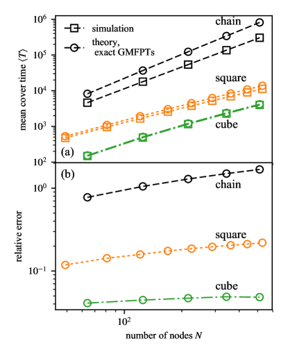
Figure 4: Example of our method yielding results with rather large deviations from simulations.(a) Mean cover time for low-dimensional $(d\leq 2)$ lattices as well as lattices in dimension $d=3$ as ($\boxempty$) an average over 1000 simulations for each data point and ($\varbigcirc$) theoretical result from exact GMFPTs computed from the unnormalized graph Laplacian’s spectrum Eq. (12). (b) The relative error is is increasing with increasing system size but is comparably lower for $d=3$ (cubes).

Network	$N$	$\left\langle k\right\rangle$	$\frac{\left\langle T^{\mathrm{sim}}\right\rangle}{N\log N}$	$\frac{\left\langle T^{\mathrm{es}}\right\rangle}{N\log N}$	$\left|1-\frac{\left\langle T^{\mathrm{sim}}\right\rangle}{\left\langle T^{\mathrm{es}}\right\rangle}\right|$	$\frac{\left\langle T^{\mathrm{ex}}\right\rangle}{N\log N}$	$\left|1-\frac{\left\langle T^{\mathrm{sim}}\right\rangle}{\left\langle T^{\mathrm{ex}}\right\rangle}\right|$
Barcelona	128	2.2	9.7	2.70	2.6	12.29	0.21
Beijing	104	2.2	10.4	2.67	2.9	16.00	0.35
Berlin	170	2.1	14.4	2.78	4.2	21.19	0.32
Chicago	141	2.1	14.8	2.74	4.4	20.02	0.26
Hong Kong	82	2.1	10.1	2.96	2.4	13.07	0.23
London	266	2.3	14.8	2.80	4.3	19.26	0.23
Madrid	209	2.3	14.4	2.67	4.4	20.42	0.29
Mexico	147	2.2	11.0	2.74	3.0	14.80	0.26
Moscow	134	2.3	12.0	2.95	3.1	14.66	0.18
New York	433	2.2	16.2	2.65	5.1	24.25	0.33
Osaka	108	2.3	9.0	2.91	2.1	11.40	0.21
Paris	299	2.4	11.4	2.85	3.0	14.22	0.20
Seoul	392	2.2	19.7	2.58	6.6	31.24	0.37
Shanghai	148	2.1	14.6	2.69	4.4	19.96	0.27
Tokyo	217	2.4	12.9	2.78	3.6	17.69	0.27

Table 2: Same procedure as in Tab. 1, but for subway networks of big cities, taken for the year 2009 from roth_long-time_2012 . These values are additionally shown in Fig. 3 (bottom).

Additionally, we performed simulations on $d$-dimensional lattices of dimension $d\in\{1,2,3\}$ (chains, squares and cubes) using node numbers $N\in\{(2n+1)^{2}:n\in\mathbb{N},\ 2\leq n\leq 12\}$ for $d=2$ and $N\in\{n^{3}:n\in\mathbb{N},4\leq n\leq 8\}$ for $d=1$ and $d=3$. For low-dimensional lattice networks with $d\leq 2$, the relaxation time is large compared to a variety of complex networks (see Fig. 1 in elsasser_tight_2011 ). Hence, we suspect that our method will not perform well for low-dimensional lattice networks and networks where nodes are embedded in low-dimensional space at position $\boldsymbol{r}_{u}$ with short-range connection probability $\pi_{vu}\propto r_{vu}^{-\omega}$ with $r_{vu}=\left|\boldsymbol{r}_{u}-\boldsymbol{r}_{v}\right|$ and $\omega>d$ as those networks are comparable to low-dimensional lattices concerning search processes kleinberg_small-world_2000 . Indeed, as can be seen in Fig. 4, the relative error between simulation and heuristic results increases with increasing $N$, up to $\approx 110\%$ for chains and $\approx 10\%$ for square lattices using exact GMFPTs, whereas smaller relative errors of up to $\approx 4\%$ are reached for cube lattices. Similar results are obtained for real-world networks embedded in a two-dimensional space with short-range connection probability such as subway networks roth_long-time_2012 (shown in Tab. 2 and Fig. 3). Here, the estimation from estimated GMFPTs systematically underestimates the cover time while using exact GMFPTs yields an overestimation of the cover time by $\approx 20\%-40\%$.

Generally, the more exact result of GMFPTs calculated via the unnormalized graph Laplacian gives results with lower relative error than using lower bound GMFPTs, as expected.

Concerning the impact of network structure on the error of our heuristic compared to the true mean cover time, we found that a large relaxation time directly influences the relative error. Since we derived our results under the assumption that the relaxation time is $t_{\mathrm{rlx}}\ll N$, we measured relative error against the ratio $t_{\mathrm{rlx}}/N$ and used Eq. (4) to find

$$\mathrm{rel.\ err.}\propto\left(\frac{\lambda_{2}^{-1}}{N}\right)^{-0.59}$$

as can be seen in Fig. 5 indicating that increasing relaxation time increases the error of our heuristic.

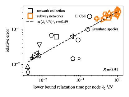
Figure 5: The relative error of our heuristic is increasing with increasing inverse second smallest eigenvalue $\lambda_{2}^{-1}$ of the unnormalized graph Laplacian, indicating that our method produces higher deviations for networks with relatively high relaxation times as per Eq. (4). Networks are marked with the same symbols as in Fig. 3.

IV Conclusions

We studied the cover time of simple discrete time random walks on single component complex networks with $N$ nodes. Treating each target node as independent from the start node, we were able to find the cumulative distribution function of the cover time by finding the maximum of $N$ drawn FPTs from the $N$ target nodes’ FPT distributions which solely depend on their GMFPT. Using this method, the complexity of finding the mean cover time of an arbitrary complex network is heavily decreased since the problem is practically reduced to finding the nodes’ GMFPTs using simple estimations or spectral methods, which is computationally much more feasible than simulating random walks starting on every node, especially for large networks.

We showed that this procedure yields reliable estimations of the mean cover time for a variety of networks where random walks decay quickly, namely ER networks, BA networks, random $k$-regular networks, and a collection of real-world networks. We furthermore showed that for low-dimensional lattices as well as networks which are embedded in low-dimensional space and have short-range connection probability, e.g. subway networks, our method does not produce reliable results. We were able to map this deviation of the heuristic result to the ratio of relaxation time per node, indicating that for networks with high relaxation time the heuristic will produce more erroneous results. The large deviations for the E. Coli interaction network and the grassland species food web is most likely related to the fact that those networks are strongly hierarchically clustered clauset_hierarchical_2008 ; ravasz_hierarchical_2002 and hence similar to low-dimensional spatial networks with short-range interaction probability concerning random walks and search processes watts_identity_2002 . The exact influence of a strong hierarchically organized network structure on cover time is, however, a task for future investigations.

Finally, note that even though we derived our results for unweighted networks, they can be easily made applicable to weighted networks and subclasses of directed networks, as they only depend on the calculation of GMFPTs. Those, in turn, depend solely on the transition matrix $W_{vu}=A_{vu}/\sum_{u}A_{vu}$ which is similarly defined for weighted and directed networks.

Appendix A The GMFPT of a complete graph

Suppose a random walker starts at any node $u$. The probability to reach any other node of the network in one time step is $p=1/(N-1)$. Looking at a single target node $v$ we want to calculate the probability that $v$ is first passaged at time $t$, which is given as

$$p_{t}=(1-p)^{t-1}p.$$

Hence, the GMFPT for every target node is

$$\tilde{\tau}=\sum_{t=1}^{\infty}tp_{t}=-p\frac{\partial}{\partial p}\frac{1}{p}=\frac{1}{p}=N-1.$$

Appendix B Continuous time approximation

Since we are investigating discrete time random walks in this study, the probability distributions are actually probability mass functions (pmfs) and expectation values should be calculated using series instead of integrals. In the following, we discuss differences and introduced errors by using continuous distributions instead.

First, the discrete time cumulative distribution function for first passage time $\tau$ at node $v$ is calculated using pmf

$$p_{v,\tau} =\exp(-\beta_{v}\tau)\Bigg{/}\sum_{t=1}^{\infty}\exp(-\beta_{v}t)$$

$$=[1-\exp(-\beta_{v})]\exp(-\beta_{v}(\tau-1)),$$

yielding

$$P(t_{v}\leq T) =\sum_{t=1}^{T}p_{v,t}=(1-\exp(-\beta_{v}))\sum_{t=1}^{T}\exp(-\beta_{v}(t-1))$$

$$=1-\exp(-\beta_{v}T)$$

which is equal to the continuous time result in Eq. (6). The mean cover time is then given as the series, respectively partial sum

$$T_{u}=\sum_{T=1}^{\infty}\left[1-P_{u}(T)\right]=\sum_{T=1}^{\infty}\bar{P}_{u}(T)\approx\sum_{T=1}^{T_{\max}}\bar{P}_{u}(T)$$

where we approximated the upper boundary using a $T_{\max}$ with $\bar{P}_{u}(T_{\max})\leq 10^{-10}$ (see App. D). This partial sum is equal to the trapezoidal approximation of the integral

$$\int\limits_{0}^{T_{\max}}\mathrm{d}T\ \bar{P}_{u}(T)=\frac{1}{2}\bar{P}_{u}(0)+\sum_{T=1}^{T\max-1}\bar{P}_{u}(T)+\frac{1}{2}\bar{P}_{u}(T_{\max})+\Phi$$

with $\Delta T=1$. Since the function $\bar{P}_{u}(T)$ has value $\bar{P}_{u}(0)=1$, using the integral instead of the sum introduces a systematic error of $1/2$. Using the first derivative $\bar{P}^{\prime}_{u}(T)$, the error $\Phi$ emerging from the trapezoidal rule can be asymptotically estimated to be

$$|\Phi|=\frac{\Delta T^{2}}{12}\left|\bar{P}^{\prime}_{u}(T_{\max})-\bar{P}^{\prime}_{u}(0)\right|$$

for $T_{\max}\rightarrow\infty$ atkinson_introduction_1989 . With

$$\bar{P}^{\prime}_{u}(T)=-\sum_{v\neq u}\beta_{v}\exp(-\beta_{v}T)\prod_{w\neq v\neq u}\left[1-\exp(-\beta_{w}T)\right]$$

we have $\bar{P}^{\prime}_{u}(0)=0$. In another way, analogous to Eq. (10) we find

$$\bar{P}_{u}(T) = \sum_{\mathcal{S\in P}^{*}(\mathcal{V}\backslash\{u\})}(-1)^{|\mathcal{S}|+1}\exp\left(-\sum_{v\in\mathcal{S}}\beta_{v}T\right)$$

$$\left|\bar{P}^{\prime}_{u}(T)\right| = \sum_{\mathcal{S\in P}^{*}(\mathcal{V}\backslash\{u\})}(-1)^{|\mathcal{S}|+1}\left(\sum_{v\in\mathcal{S}}\beta_{v}\right)\exp\left(-\sum_{v\in\mathcal{S}}\beta_{v}T\right).$$

For most nodes the decay rates are $\beta_{v}\lessapprox N^{-1}$ with $\lessapprox$ meaning “lower or of similar order”. Then $\sum_{v\in\mathcal{S}}\beta_{v}\lessapprox 1$ and hence $\left|\bar{P}^{\prime}_{u}\right|\lessapprox\bar{P}_{u}$ such that one can safely assume $\left|\bar{P}^{\prime}_{u}(T_{\max})\right|\lessapprox\bar{P}_{u}(T_{\max})\leq 10^{-10}$ yielding absolute error

$$|\Phi|\lessapprox 10^{-11}.$$

Appendix C Approximation of mean cover time integral

In the following, we show that instead of solving integral Eq. (8), one can safely use Eq. (10). We do so by calculating the total difference between both as

$$\Theta =\int\limits_{0}^{\infty}\mathrm{d}T\left[1-P(T)\right]-$$

$$\qquad-\int\limits_{0}^{\infty}\mathrm{d}T\left[1-P(T)\frac{1}{N}\sum_{v=1}^{N}\frac{1}{1-\exp(-\beta_{v}T)}\right]$$

$$=\int\limits_{0}^{\infty}\mathrm{d}T\ P(T)\left[Q(T)-1\right],$$ (15)

defining $Q(T)=\frac{1}{N}\sum_{v=1}^{N}\left(1-\exp(-\beta_{v}T)\right)^{-1}$. Note that the cover time cdf $P(T)$ is given by Eq. (9), s.t. both

$$\lim_{T\rightarrow 0}P(T) =0$$

$$\lim_{T\rightarrow 0}P(T)Q(T) =0$$

and

$$\lim_{T\rightarrow\infty}P(T) =1$$

$$\lim_{T\rightarrow\infty}P(T)Q(T) =1,$$

meaning that for both integration limits, the integrand approaches 0. In the following we assume that the distribution of decay rates is relatively homogeneous in the region of small rates, implying that there is a low number $1<n\ll N$ of nodes $i\in\mathcal{V}_{\mathrm{small}}$ with $n=|\mathcal{V}_{\mathrm{small}}|$ that are of the same order as $\beta_{\min}=\min\{\beta_{v}:v\in\mathcal{V}\}$. This is a relatively safe assumption for most network models and real-world networks as in most cases there are more nodes with small degree (hence small decay rates) than nodes with high degree (hence high decay rates). Now suppose the integration approaches a time where $T\approx\beta_{\min}^{-1}$, implying that, while most terms $1-\exp(-T\beta_{v\notin\mathcal{V}_{\mathrm{small}}})$ are virtually equal to 1 there are still $n$ terms $1-\exp(-T\beta_{i})<1$, such that $P(T)\approx\prod_{i\in\mathcal{V}_{\mathrm{small}}}^{n}(1-\exp(-T\beta_{i}))\ll 1.$ Furthermore, there will already be a majority of terms $1-\exp(-T\beta_{v})\rightarrow 1$ which leads to $Q(T)$ approaching $Q(T)\stackrel{{\scriptstyle N\gg 1}}{{\longrightarrow}}1$. Hence, we can safely assume that for a network with a larger number of nodes the integrand approaches zero at all times while the global mean cover time grows quickly and thus the relative error of Eq. (10) is approaching

$$\frac{\Theta}{\left\langle T\right\rangle}\stackrel{{\scriptstyle N\gg 1}}{{\longrightarrow}}0.$$

In particular, we can calculate the error between the integrals for random networks with constant GMFPT $\tilde{\tau}$ for every node, which is given as

$$\tilde{\Theta} = \tilde{\tau}_{N+1}\Big{[}\gamma+\psi(N+1)\Big{]}-\tilde{\tau}_{N}\Big{[}\gamma+\psi(N)\Big{]}$$

$$\approx \tilde{\tau}_{N}\log\left(\frac{N}{N-1}\right)\approx\tilde{\tau}_{N}\frac{1}{N}$$

Where we used $\psi(N+1)=\log N+\mathcal{O}(N^{-1})$ and assumed $\tilde{\tau}_{N}\sim\tilde{\tau}_{N+1}$. Consequently, we can find the relative error to be approximately

$$\frac{\tilde{\Theta}}{\left\langle T\right\rangle}\approx\frac{1}{N\gamma+N\log(N-1)}\sim\frac{1}{N\log N}.$$ (16)

Even though this relation is derived for the special case of networks where every node has the same GMFPT, a numerical analysis of Eq. (15) reveals that this scaling relation holds approximately for all networks investigated in this study, as can be seen in Fig. (6).

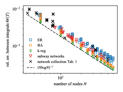
Figure 6: Relative error Eq. (15) between integrals Eq. (8) and Eq. (10) for all networks investigated in this study besides lattices. For each network we show the relative error for both sets of rates, $\tau_{v}^{\mathrm{es}}$ and $\tau_{v}^{\mathrm{ex}}$. For ER, BA and random $k$-regular networks, we built means over the largest components of 100 network realizations for $\left\langle k\right\rangle\in\{3,5,7,9\}$ and $m\in\{3,5,7,9\}$, respectively. The measured relative errors are roughly following the scaling relation Eq. (16).

Appendix D Simulations and numerical evaluations of the mean cover time

The code used for the random walk simulations is a standard implementation of discrete time random walks on networks and available online as a C++/Python/Matlab package, see maier_cnetworkdiff_2017 .

In order to evaluate the mean cover time, the integrals Eqs. (11) and (12) were solved numerically. Note that for the numerical integration, an upper integration bound of infinity can be problematic when the decay region of the integrand is unknown. Hence, we chose an upper integration limit $T_{\max}$ where $1-P(T_{\max})\leq 10^{-10}$. The code is available online as a Python package, see maier_nwdiff_2017 . For solving the integral Eq. (12) we computed the GMFPT of each node via Eq. (2) with eigenvalues and -vectors computed using the NumPy implementation jones_scipy:_2001 of the standard algorithm for eigenvalue and -vector computation of Hermitian matrices strang_linear_1980 .

References

- (1) B. Øksendal, Stochastic differential equations: An introduction with applications. Universitext, Berlin: Springer, 1992. OCLC: 246776666.
- (2) H. C. Berg, Random walks in biology. Princeton, NJ: Princeton University Press, 1993.
- (3) A. Barrat, M. Barthelemy, and A. Vespignani, Dynamical processes on complex networks. Cambridge, UK ; New York: Cambridge University Press, 2008. OCLC: ocn231581094.
- (4) D. Brockmann, “Anomalous diffusion and the structure of human transportation networks,” The European Physical Journal Special Topics, vol. 157, no. 1, pp. 173–189, 2008.
- (5) M. Newman, Networks: An introduction. New York, NY, USA: Oxford University Press, Inc., 2010.
- (6) J. Klafter and I. M. Sokolov, First steps in random walks: from tools to applications. Oxford ; New York: Oxford University Press, 2011. OCLC: ocn714724924.
- (7) N. Masuda, M. A. Porter, and R. Lambiotte, “Random walks and diffusion on networks,” arXiv:1612.03281 [cond-mat, physics:physics], Dec. 2016. arXiv: 1612.03281.
- (8) L. Hufnagel, D. Brockmann, and T. Geisel, “Forecast and control of epidemics in a globalized world,” Proceedings of the National Academy of Sciences of the United States of America, vol. 101, pp. 15124–15129, Oct. 2004.
- (9) D. Brockmann and D. Helbing, “The hidden geometry of complex, network-driven contagion phenomena,” Science (New York, N.Y.), vol. 342, no. 6164, pp. 1337–1342, 2013.
- (10) F. Iannelli, A. Koher, D. Brockmann, P. Hövel, and I. M. Sokolov, “Effective distances for epidemics spreading on complex networks,” Physical Review E, vol. 95, p. 012313, Jan. 2017.
- (11) L. Page, S. Brin, R. Motwani, and T. Winograd, “The PageRank Citation Ranking: Bringing Order to the Web, http://ilpubs.stanford.edu:8090/422/,” Technical Report 1999-66, Stanford InfoLab, Nov. 1999.
- (12) M. D. Domenico, A. Solé-Ribalta, S. Gómez, and A. Arenas, “Navigability of interconnected networks under random failures,” Proceedings of the National Academy of Sciences, vol. 111, pp. 8351–8356, Oct. 2014.
- (13) C. Cooper and A. Frieze, “The cover time of sparse random graphs,” Random Structures and Algorithms, vol. 30, pp. 1–16, Jan. 2007.
- (14) C. Cooper and A. Frieze, “The cover time of the preferential attachment graph,” Journal of Combinatorial Theory, Series B, vol. 97, no. 2, pp. 269–290, 2007.
- (15) L. Lovász, “Random walks on graphs: a survey,” in Combinatorics, Paul Erdős is Eighty (D. Miklós, V. T. Sós, and T. Szőnyi, eds.), vol. 2, pp. 353–398, Budapest: János Bolyai Mathematical Society, 1996.
- (16) Y. Lin, A. Julaiti, and Z. Zhang, “Mean first-passage time for random walks in general graphs with a deep trap,” The Journal of Chemical Physics, vol. 137, p. 124104, Sept. 2012.
- (17) H. W. Lau and K. Y. Szeto, “Asymptotic analysis of first passage time in complex networks,” EPL (Europhysics Letters), vol. 90, no. 4, p. 40005, 2010.
- (18) B. Mohar, “Some applications of Laplace eigenvalues of graphs,” in Graph Symmetry, NATO ASI Series, pp. 225–275, Springer, Dordrecht, 1997.
- (19) B. F. Maier, “B.F. Maier’s FB friends network, https://github.com/benmaier/BFMaierFBnetwork,” Apr. 2017.
- (20) D. J. Watts and S. H. Strogatz, “Collective dynamics of ’small-world’ networks,” Nature, vol. 393, pp. 440–442, June 1998.
- (21) S. S. Shen-Orr, R. Milo, S. Mangan, and U. Alon, “Network motifs in the transcriptional regulation network of Escherichia coli,” Nature Genetics, vol. 31, no. 1, pp. 64–68, 2002.
- (22) R. Cross and A. Parker, The hidden power of social networks. Boston, MA: Harvard Business School Press, 2004.
- (23) D. Lusseau, K. Schneider, O. J. Boisseau, P. Haase, E. Slooten, and S. M. Dawson, “The bottlenose dolphin community of Doubtful Sound features a large proportion of long-lasting associations,” Behavioral Ecology and Sociobiology, vol. 54, pp. 396–405, Sept. 2003.
- (24) M. Girvan and M. E. J. Newman, “Community structure in social and biological networks,” Proceedings of the National Academy of Sciences of the United States of America, vol. 99, pp. 7821–7826, June 2002.
- (25) H. A. Dawah, B. A. Hawkins, and M. F. Claridge, “Structure of the Parasitoid Communities of Grass-Feeding Chalcid Wasps,” Journal of Animal Ecology, vol. 64, no. 6, pp. 708–720, 1995.
- (26) W. W. Zachary, “An information flow model for conflict and fission in small groups,” Journal of Anthropological Research, vol. 33, pp. 452–473, 1977.
- (27) D. E. Knuth, The Stanford GraphBase: A platform for combinatorial computing. Reading, MA: Addison-Wesley, 1993.
- (28) C. Aicher, A. Z. Jacobs, and A. Clauset, “Learning latent block structure in weighted networks,” Journal of Complex Networks, vol. 3, pp. 221–248, June 2015.
- (29) V. Krebs, “Mapping networks of terrorist cells,” Connections, vol. 24, pp. 43–52, 2002.
- (30) V. Colizza, R. Pastor-Satorras, and A. Vespignani, “Reaction-diffusion processes and metapopulation models in heterogeneous networks,” Nature Physics, vol. 3, pp. 276–282, Apr. 2007.
- (31) A. Steger and N. C. Wormald, “Generating random regular graphs quickly,” Comb. Probab. Comput., vol. 8, pp. 377–396, July 1999.
- (32) C. Roth, S. M. Kang, M. Batty, and M. Barthelemy, “A long-time limit for world subway networks,” Journal of The Royal Society Interface, 2012.
- (33) R. Elsässer and T. Sauerwald, “Tight bounds for the cover time of multiple random walks,” Theoretical Computer Science, vol. 412, pp. 2623–2641, May 2011.
- (34) J. Kleinberg, “The Small-world Phenomenon: An Algorithmic Perspective,” in Proceedings of the Thirty-second Annual ACM Symposium on Theory of Computing, STOC ’00, (New York, NY, USA), pp. 163–170, ACM, 2000.
- (35) A. Clauset, C. Moore, and M. E. J. Newman, “Hierarchical structure and the prediction of missing links in networks,” Nature, vol. 453, no. 7191, pp. 98–101, 2008.
- (36) E. Ravasz, A. L. Somera, D. A. Mongru, Z. N. Oltvai, and A.-L. Barabási, “Hierarchical Organization of Modularity in Metabolic Networks,” Science, vol. 297, pp. 1551–1555, Aug. 2002.
- (37) D. J. Watts, P. S. Dodds, and M. E. J. Newman, “Identity and Search in Social Networks,” Science, vol. 296, pp. 1302–1305, May 2002.
- (38) K. E. Atkinson, An introduction to numerical analysis. New York: Wiley, 2nd ed., 1989.
- (39) B. F. Maier, “cNetworkDiff - A C++/Python/MATLAB package for random walk simulations on networks, https://github.com/benmaier/cNetworkDiff,” Sept. 2017.
- (40) B. F. Maier, “nwDiff - A Python package for random walk simulations and heuristic calculations of random walk observables on networks, https://github.com/benmaier/nwDiff,” Sept. 2017.
- (41) E. Jones, T. Oliphant, P. Peterson, and others, SciPy: Open source scientific tools for Python. 2001.
- (42) G. Strang, Linear algebra and its applications. Belmont, CA: Thomson, Brooks/Cole, 2nd ed., 1980.