Extending the modeling of the anisotropic galaxy power spectrum to $k=0.4\ h\mathrm{Mpc}^{-1}$

Abstract

We present a new model for the redshift-space power spectrum of galaxies and demonstrate its accuracy in modeling the monopole, quadrupole, and hexadecapole of the galaxy density field down to scales of $k=0.4\ h\text{Mpc}^{-1}$. The model describes the clustering of galaxies in the context of a halo model and the clustering of the underlying halos in redshift space using a combination of Eulerian perturbation theory and $N$-body simulations. The modeling of redshift-space distortions is done using the so-called distribution function approach. The final model has 13 free parameters, and each parameter is physically motivated rather than a nuisance parameter, which allows the use of well-motivated priors. We account for the Finger-of-God effect from centrals and both isolated and non-isolated satellites rather than using a single velocity dispersion to describe the combined effect. We test and validate the accuracy of the model on several sets of high-fidelity $N$-body simulations, as well as realistic mock catalogs designed to simulate the BOSS DR12 CMASS data set. The suite of simulations covers a range of cosmologies and galaxy bias models, providing a rigorous test of the level of theoretical systematics present in the model. The level of bias in the recovered values of $f\sigma_{8}$ is found to be small. When including scales to $k=0.4\ h\mathrm{Mpc}^{-1}$, we find 15-30% gains in the statistical precision of $f\sigma_{8}$ relative to $k=0.2\ h\mathrm{Mpc}^{-1}$ and a roughly 10-15% improvement for the perpendicular Alcock-Paczynski parameter $\alpha_{\perp}$. Using the BOSS DR12 CMASS mocks as a benchmark for comparison, we estimate an uncertainty on $f\sigma_{8}$ that is $\sim$10-20% larger than other similar Fourier-space RSD models in the literature that use $k\leq 0.2\ h\mathrm{Mpc}^{-1}$, suggesting that these models likely have a too-limited parametrization.

1 Introduction

Galaxy redshift surveys measure the three-dimensional clustering of galaxies in the Universe, and over the past few decades, they have provided a wealth of cosmological information [1, 2, 3, 4, 5, 6, 7, 8, 9]. In combination with other cosmological probes, such as observations of the cosmic microwave background, type-Ia supernova samples, and weak-lensing surveys, analyses of the large-scale structure (LSS) of the Universe have proven invaluable in establishing the current cosmological paradigm, the $\Lambda$CDM model, as well as measuring its parameters with ever-increasing precision.

Crucial to the success of galaxy surveys has been the ability to precisely and accurately measure the feature imprinted on the clustering of galaxies by baryon acoustic oscillations in the early Universe (BAO; see e.g., [10] for a review). The BAO signal can be used to provide constraints on the expansion history of the Universe and infer properties of dark energy (e.g., [11, 12]). The isotropic effect was first detected in the SDSS [5] and the 2dFGRS [4], and more recent measurements of the anisotropic signal, combined with the Alcock-Paczynski (AP; [13]) effect, have provided percent-level measurements of the Hubble parameter $H(z)$ and angular diameter distance $D_{a}(z)$ [9]. Perhaps most encouragingly, the BAO signal is well-understood theoretically, with systematic effects on the distance scale expected to be sub-dominant for future generations of surveys [14, 15, 16, 17, 18].

Beyond the BAO signal, additional information is present in the clustering of galaxies through what are known as redshift-space distortions (RSD). The peculiar velocities of galaxies affect their measured redshifts through the Doppler effect, and in turn, these measured redshifts are used to infer the line-of-sight (LOS) position of those galaxies. The peculiar velocity field is sourced by the gravitational potential, and thus, an anisotropic signal containing information about the rate of structure growth in the Universe is imprinted on the clustering. Extracting information from RSD is inherently more difficult than with BAO, as it requires modeling of the full broadband shape of the clustering statistic and precise understanding of the anisotropy induced by RSD. The theoretical task is complicated by the fact that the well-understood, linear Kaiser model [19] breaks down on relatively large scales, with various kinds of nonlinear effects complicating the theoretical modeling (e.g., [20, 21, 22, 23]). Of particular importance is the large, nonlinear virial motions of satellite galaxies within halos, known as the Finger-of-God (FoG) effect [24]. Since the statistical precision of clustering measurements is generally higher on smaller scales, where the effects of nonlinearities are worse, a direct limit on the amount of useable cosmological information is imposed due to theoretical uncertainties.

Despite these modeling challenges, RSD analyses have developed into one of the most popular and powerful cosmological probes today [25, 26, 27, 28, 29, 30, 31, 32, 33, 34, 35, 36]. Constraints on the growth rate of structure through measurements of the parameter combination $f(z)\sigma_{8}(z)$ can provide tests of General Relativity (e.g., [28]), as well as information about the properties of neutrinos [37, 35] and tighter constraints on the expansion history through the AP effect (e.g., [12]). Recent results from Data Release 12 (DR12) of the Baryon Oscillation Spectroscopic Survey (BOSS) [38, 39, 40, 41] have provided the tightest constraints to date on the growth rate of structure, with roughly 10% constraints on $f\sigma_{8}(z_{\mathrm{eff}})$ in 3 redshift bins centered at $z_{\mathrm{eff}}=0.38$, $0.51$, and $0.61$.

To date, RSD analyses have generally either relied directly on the results of $N$-body simulations or on perturbative approaches to model the clustering of galaxies in the quasi-linear and nonlinear regimes. Both approaches have their pros and cons. For simulation-based analyses, e.g., [42, 43, 36, 44], the simulations represent the best possible description of nonlinearities, although individual simulations are expensive to run and, often, the relevant parameter space cannot be as sufficiently explored as one would like. On the other hand, modeling techniques relying on perturbation theory (PT), e.g., [39, 45, 41, 38], are relatively fast to compute but will always break down on small enough scales and fail to capture non-perturbative features, such as the FoG effect from satellites. In either case, simulations play a crucial role in estimating the range of scales where a model remains accurate enough to recover cosmological parameters in an unbiased fashion.

In this work, we present a new model for the redshift-space power spectrum of galaxies, describing the galaxy clustering in the context of a halo model [46, 47, 48, 49] and relying on a combination of Eulerian PT and $N$-body simulations to model the power spectrum of dark matter halos in redshift space. We use several sets of $N$-body simulations to validate our model, and we perform cosmological parameter analyses on realistic BOSS-like mock catalogs to verify both the accuracy and constraining power of the model. The model relies on the distribution function approach [50, 51, 52, 53, 54, 55] to map real-space statistics to redshift space. This formalism is different but complementary from other commonly-used approaches in RSD analyses, such as the TNS model [56] or the Gaussian streaming model [57]. We build upon the results presented in [58], which showed that the characterization of the redshift-space power spectrum of galaxies in terms of 1-halo and 2-halo correlations is accurate when compared against $N$-body simulations. We extend that work by improving the accuracy of the underlying model for the halo redshift-space power spectrum. The model is based on the PT results presented in [54], but uses simulation-based modeling for key terms. In particular, we develop and extend the Halo-Zel’dovich Perturbation Theory (HZPT) of [59], which relies on a combination of linear Lagrangian PT and simulation-based calibration. A Python software package pyRSD that implements the model described in this work is publicly available.

This paper is organized as follows. Section 2 describes the set of simulations that we use to calibrate our model, as well as the test suite that we use for independent validation. We describe the power spectrum estimator, covariance matrix, and likelihood analysis used to perform parameter estimation in section 3. In section 4, we detail the power spectrum model, first reviewing the halo model formalism presented in [58] and then discussing several new modeling approaches for the redshift-space halo power spectrum. We assess the accuracy and performance of the model based on an independent test suite of simulations in section 5. Finally, we discuss our results and future prospects in section 6 and conclude in section 7.

Name	$L_{\mathrm{box}}$ $[\ h^{-1}\text{Mpc}]$	$z_{\mathrm{box}}$	$\Omega_{m}$	$\Omega_{b}h^{2}$	$h$	$n_{s}$	$\sigma_{8}$
RunPB	1380	0.55	0.292	0.022	0.69	0.965	0.82
N-series; Challenge D,E	2600	0.562	0.286	0.02303	0.7	0.96	0.82
Challenge A,B,F,G	2500	0.5	0.30711	0.022045	0.6777	0.96	0.82
Challenge C	2500	0.441	0.27	0.02303	0.7	0.96	0.82

Table 1: The cosmological and simulation parameters for the various $N$-body simulations used in this work.

2 Simulations

We use several sets of $N$-body simulations for both calibrating and testing the model presented in this paper. The first set of simulations, described in section 2.1, is used heavily in verifying individual components of the clustering model. Sections 2.2 and 2.3 describe an independent suite of high-fidelity simulations that we use to independently verify the accuracy and precision of the model. The relevant cosmological and simulation parameters for the mocks discussed in this section are summarized in table 1.

2.1 RunPB

The main set of simulations used for calibration and testing purposes is the RunPB $N$-body simulation produced by Martin White with the TreePM N-body code of [60]. These simulations have been used recently in a number of analyses [61, 36, 62, 63]. The simulation set has 10 realizations of $2048^{3}$ dark matter particles in a cubic box of length $L=1380\ h^{-1}\text{Mpc}$. The cosmology is a flat $\Lambda$CDM model with $\Omega_{b}h^{2}$ = 0.022, $\Omega_{m}$ = 0.292, $n_{s}$ = 0.965, $h$ = 0.69 and $\sigma_{8}=0.82$.

For testing and calibration of the modeling of halo clustering, we use halo catalogs generated using a friends-of-friends (FOF) algorithm with a linking length of 0.168 times the mean particle separation to identify halos [64]. We consider 8 halo mass bins (as a function of $M_{\text{fof}}$) across 10 redshift outputs, ranging from $z=0$ to $z=1$. The redshift outputs considered are: $z\in\{0,0.1,0.25,0.4,0.5,0.55,0.65,0.75,1\}$. The (overlapping) halo mass bins range from $\mathrm{log}_{10}M_{\mathrm{fof}}=12.6$ to $\mathrm{log}_{10}M_{\mathrm{fof}}=14.4$ and are described in table 2. For reference, table 2 also gives the linear bias values at $z=0.55$ and $z=0$. The linear biases for each halo mass bin are determined from the ratio of the large-scale halo-matter cross power spectrum to the matter power spectrum at each redshift output.

bin	1	2	3	4	5	6	7	8
$\log_{10}M_{\mathrm{fof}}^{\mathrm{min}}$	12.6	12.8	13.0	13.2	13.4	13.6	13.8	14.0
$\log_{10}M_{\mathrm{fof}}^{\mathrm{max}}$	13.0	13.2	13.4	13.6	13.8	14.0	14.2	14.4
$b_{1}(z=0.55)$	1.40	1.56	1.78	2.04	2.36	2.77	3.28	3.93
$b_{1}(z=0)$	1.00	1.07	1.19	1.33	1.51	1.74	2.03	2.41

Table 2: The halo mass bins used when comparing results from the RunPB simulations to theoretical modeling of halo clustering. For each of the 10 redshift outputs ranging from $z=0$ to $z=1$, we consider 8 fixed halo mass bins. We give the corresponding large-scale, linear bias for each bin for two redshifts, $z=0.55$ and $z=0$.

We also rely heavily on a set of galaxy catalogs produced using halo occupation distribution (HOD) modeling from halo catalogs generated from the $z=0.55$ RunPB realizations. The halo catalog production and the HOD modeling is the same as in [36]: halos are identified using a spherical overdensity (SO) algorithm and the HOD parameterization follows [65]. In [36], the RunPB simulations are denoted as the MedRes simulations. The HOD parameters used to generate the galaxy catalog used in this work are $\{\log_{10}M_{\mathrm{min}},\sigma_{\log_{10}M},\log_{10}M_{1},\alpha,\log_{10}M_{\mathrm{cut}}\}=\{12.99,0.308,14.08,0.824,13.20\}$. These HOD parameters were chosen to reproduce the clustering of the BOSS CMASS sample [66], i.e., a large-scale linear bias of $b_{1}\sim 2$ at $z\sim 0.5$.

2.2 N-series

The N-series cubic boxes are a set of realizations from a large-volume, high-resolution $N$-body simulation, used as part of a “mock challenge“ testing procedure by the BOSS collaboration in preparation for publishing results as part of DR12 in [9]. Details of this mock challenge can be found in [67]. Briefly, the N-series suite consists of seven independent, periodic box realizations with the same cosmology, and a side length of $L_{\mathrm{box}}=2600\ h\text{Mpc}^{-1}$ at a redshift $z_{\mathrm{box}}=0.5$. The cosmology is given by: $\Omega_{m}=0.286$, $\Omega_{\Lambda}=0.714$, $\sigma_{8}=0.82$, $n_{s}=0.96$, and $h=0.7$. The $N$-body simulation was run using the GADGET2 code [68], with sufficient mass and spatial resolution to resolve the halos that typical BOSS galaxies occupy. A single galaxy bias model was assumed, and HOD modeling was used to populate halos from the seven realizations with galaxies. The parameters of the HOD were chosen to reproduce the clustering of the BOSS CMASS sample (i.e., linear bias $b_{1}\sim 2$ at $z\sim 0.5$).

An additional set of 84 mock catalogs were generated from the three orthogonal projections of each of the seven N-series cubic boxes using the make_survey software [69]. Denoted as the “cutsky” mocks, these mocks have the same angular and radial selection function as the NGC DR12 CMASS sample [70, 9]. They model the true geometry, volume, and redshift distribution of the CMASS NGC sample and provide a realistic simulation of the true BOSS data set. Each catalog is an independent realization, and these mocks were also used as part of the DR12 mock challenge.

2.3 Lettered Challenge Boxes

A second part of the BOSS DR12 mock challenge was performed on a suite of HOD galaxy samples constructed from a heterogeneous set of high-resolution $N$-body simulations. There are seven different HOD galaxy catalogs, constructed from large-volume periodic simulation boxes with varying cosmologies. The seven catalogs are labeled A through G. Several of the boxes are based on the Big MultiDark simulation [71]. The catalogs are constructed out of simulation boxes with a range of 3 underlying cosmologies, and boxes with the same cosmology have varying galaxy bias models, which varies the overall galaxy bias by $\pm$5%. The redshift of the boxes ranges from $z=0.441$ to $z=0.562$.

These cases were designed to quantify the sensitivity of RSD models to the specifics of the galaxy bias model over a reasonable range of cosmologies, testing for any possible theoretical systematics. The cosmology and relevant simulation parameters for each of these boxes is given in table 1. A comparison of the results from the mock challenge in context of the BOSS DR12 results is presented in [9], and individual Fourier-space clustering results from the challenge are discussed in [39, 40].

3 Analysis methods

In this work, we measure the 2-point clustering of galaxies as characterized by the power spectrum multipoles, defined in terms of the 2D anisotropic power spectrum as

$$P_{\ell}(k)=\frac{2\ell+1}{2}\int_{-1}^{1}d\mu P(k,\mu)\mathcal{L}_{\ell}(\mu),$$ (3.1)

where $\mathcal{L}_{\ell}$ is the Legendre polynomial of order $\ell$. We estimate the multipoles from catalogs of discrete galaxies in periodic box $N$-body simulations and from more realistic, cutsky mock catalogs, which mimic real survey data. We estimate the continuous galaxy overdensity field using a Triangular Shaped Cloud interpolation scheme (see e.g., [72]) to assign the galaxy positions to a 3D Cartesian grid.

For both periodic boxes and cutsky mocks, we employ Fast Fourier Transform (FFT) based estimators to compute the multipoles. In the case of simulation boxes with periodic boundary conditions, the line-of-sight is assigned to a specific box axis and the power spectrum $P(k,\mu)$ can be computed as the square of the Fourier modes of the overdensity field. The desired multipoles are then found by computing equation 3.1 as a discrete sum over $P(k,\mu)$. In the case of the cutsky mocks, we employ the FFT-based estimator described in [73], which modifies the FFT estimator presented by [74] and [75]. Building on the ideas of previous power spectrum estimators [76, 77], this estimator uses a spherical harmonic decomposition to allow the use of FFTs to compute the higher-order multipoles, with 5 and 9 FFTs required to compute the quadrupole and hexadecapole, respectively. When computing FFTs, we ensure that the grid configuration is such that our desired maximum wavenumber is not greater than one-half of the Nyquist frequency of the grid, which should eliminate any aliasing effects on our measured power spectra (i.e., [78]). The measured power spectra are estimated on a discrete $k$-grid which makes the angular distribution of Fourier modes irregular. This discreteness effect is especially important at low $k$ and can be accounted for by modifying equation 3.1 as

$$P_{\ell}(k)=\frac{2\ell+1}{2}\int_{-1}^{1}d\mu P(k,\mu)\frac{N_{\mathrm{modes}}(k,\mu)}{N_{\mathrm{bin}}(k)}\mathcal{L}_{\ell}(\mu),$$ (3.2)

where the $N(k,\mu)$ gives the total number of modes on the $k$-space grid, and the normalization is

$$N_{\mathrm{bin}}(k)=\int_{-1}^{1}d\mu N_{\mathrm{modes}}(k,\mu).$$ (3.3)

When computing the theoretical multipoles with the model in this work, which we compare to simulation results, we use equation 3.2 to account for the discreteness effect present in the simulation multipoles. This procedure has been shown to sufficiently correct for this effect [39]. For all power spectrum calculations, we use the publicly-available software package nbodykit [79], which uses massively parallel implementations of these estimators for fast calculations optimized to run on high-performance computing machines.

We use the Markov chain Monte Carlo (MCMC) technique to derive the likelihood distributions of the model parameters described in detail in section 4.4. We employ a modified version of the Python code emcee [80] to explore the relevant model parameter space. The data vector used in these fits is the concatenation of the monopole, quadrupole, and hexadecapole,

$$\mathcal{D}=\left[P_{0}(k),P_{2}(k),P_{4}(k)\right],$$ (3.4)

where we have measured the multipoles from simulations as previously described. The inclusion of the hexadecapole $P_{4}(k)$ has been shown to offer significant improvements on RSD constraints, i.e., [39, 40]. In all fits, we use a bin spacing in wavenumber of $\Delta k=0.005\ h\text{Mpc}^{-1}$, and the maximum wavenumber included in the fits ranges from $k_{\mathrm{max}}=0.2\ h\text{Mpc}^{-1}$ to $k_{\mathrm{max}}=0.4\ h\text{Mpc}^{-1}$. The likelihood fits require an estimate of the covariance matrix, and we use the theoretical Gaussian covariance for the multipoles in Fourier space (i.e., [45]). In the case of the cutsky mocks, we properly account for the redshift distribution and survey volume of the mock catalogs when computing the expected covariance, using e.g., [77]. Our choice for covariance matrix ignores non-Gaussian contributions produced by e.g., nonlinear structure growth, and in the case of the cutsky mocks, correlations induced by the window function due to the survey geometry. We have tested the impact of this choice for covariance matrix by comparing the parameter fits obtained when using a covariance matrix derived from a set of 1000 mock catalogs from the Quick Particle Mesh (QPM; [69]) simulations. While we do find variations in the best-fit parameters found when using the simulation-based covariance, the shifts are consistent with the derived errors.

4 The power spectrum model

In this section, we present the model for the anisotropic clustering of galaxies in Fourier space, as characterized by the broadband, two-dimensional power spectrum. First, we connect the clustering of galaxies to the clustering of halos, reviewing the halo model formalism presented in [58] in §4.1. We describe our model for the redshift-space halo power spectrum and the various modeling improvements from past work in §4.2. In §4.3, we discuss how we account for various observational effects when modeling real galaxy survey data. Finally, we summarize the complete set of model parameters in §4.4.

4.1 Halo model formalism for galaxies

Our treatment of the clustering of galaxies is based upon the model presented in [58]. The clustering of a given galaxy sample is considered within the context of a halo model [46, 48, 47, 81, 49], which allows one to separately consider contributions to the clustering arising from galaxies within the same halo and those from separate halos, known as the 1-halo and 2-halo terms, respectively. This formalism is ideal when accounting for the effects of satellite galaxies on the anisotropic power spectrum, where the radial distribution of satellites induces both 1-halo and 2-halo effects. We describe the relevant model details from [58], used in this work, below.

4.1.1 Galaxy sample decomposition

In redshift space, we can decompose contributions to the galaxy overdensity field $\delta_{g}^{S}$ into contributions from central and satellite galaxies as

$$\delta_{g}^{S}(\mathbf{k})=(1-f_{s})\delta_{c}^{S}(\mathbf{k})+f_{s}\delta_{s}^{S}(\mathbf{k}),$$ (4.1)

where $f_{s}=N_{s}/N_{g}=1-N_{c}/N_{g}$ is the satellite fraction, $N_{c}$ and $N_{s}$ are the numbers of central and satellite galaxies, respectively, and $N_{g}=N_{c}+N_{s}$ is the total number of galaxies. It follows then that the power spectrum of the galaxy density field $(2\pi)^{3}P_{gg}^{S}(\mathbf{k})\delta(\mathbf{k}+\mathbf{k}^{\prime})\equiv\left\langle\delta_{g}^{S}(\mathbf{k})\delta_{g}^{S}(\mathbf{k}^{\prime})\right\rangle$ can be expressed as

$$P^{S}_{gg}(\mathbf{k})=(1-f_{s})^{2}P^{S}_{cc}(\mathbf{k})+2f_{s}(1-f_{s})P^{S}_{cs}(\mathbf{k})+f_{s}^{2}P^{S}_{ss}(\mathbf{k}),$$ (4.2)

where $P^{S}_{cc}$, $P^{S}_{cs}$, and $P^{S}_{ss}$ are the centrals auto power spectrum, the central-satellite cross power spectrum, and the satellite auto power spectrum in redshift space, respectively.

To fully separate 1-halo and 2-halo contributions to the power spectrum, we further decompose the central and satellite galaxy samples. We decompose the central galaxy density field into those centrals that do and do not have a satellite galaxy in the same halo, denoted as types “A” and “B” centrals, respectively. For the latter type, a 1-halo contribution will exist due to the central-satellite correlations inside the same halo. We use a similar decomposition for satellite galaxies, where we consider satellites that only have a single satellite in a halo (type “A”) and those satellites that live in halos with more than one satellite (type “B”). The latter type will contribute a 1-halo term to the power spectrum, due to correlations between multiple satellites in the same halo.

With these galaxy sample definitions, we can express the central-satellite and satellite-satellite power spectra in terms of 1-halo and 2-halo correlations. Note that by construction, a halo can only have a single central galaxy, and thus, the centrals auto spectrum is a purely 2-halo contribution. The central-satellite cross power spectrum can be expressed as

$$P^{S}_{cs}(\mathbf{k}) =(1-f_{c_{B}})P^{S}_{c_{A}s}(\mathbf{k})+f_{c_{B}}P^{S}_{c_{B}s}(\mathbf{k}),$$

$$=(1-f_{c_{B}})\left[(1-f_{s_{B}})P^{S}_{c_{A}s_{A}}+f_{s_{B}}P^{S}_{c_{A}s_{B}}\right]+f_{c_{B}}\left[(1-f_{s_{B}})P^{S}_{c_{B}s_{A}}+f_{s_{B}}P^{S}_{c_{B}s_{B}}\right],$$ (4.3)

where $f_{c_{B}}=N_{c_{B}}/N_{c}$ is the fraction of centrals that have a satellite in the same halo, and $f_{s_{B}}=N_{s_{B}}/N_{s}$ is the fraction of satellites that live in halos with more than one satellite. Because the sample $c_{B}$ consists of central galaxies that have satellite galaxies inside the same halo, the term $P^{S}_{c_{B}s}$ (and similarly, $P^{S}_{c_{B}s_{A}}$ and $P^{S}_{c_{B}s_{B}}$) contains a 1-halo contribution, so we write it as $P^{S}_{c_{B}s}=P^{S,1h}_{c_{B}s}+P^{S,2h}_{c_{B}s}$. All other power spectra terms in equation 4.3 are purely 2-halo contributions.

Similarly, we can express the satellite auto power spectrum as

$$P^{S}_{ss}(\mathbf{k})=(1-f_{s_{B}})^{2}P^{S}_{s_{A}s_{A}}(\mathbf{k})+2f_{s_{B}}(1-f_{s_{B}})P^{S}_{s_{A}s_{B}}(\mathbf{k})+f_{s_{B}}^{2}P^{S}_{s_{B}s_{B}}(\mathbf{k}).$$ (4.4)

As in the case of $P^{S}_{c_{B}s}$, the term $P^{S}_{s_{B}s_{B}}$ includes both 1-halo and 2-halo contributions, which we can express as $P^{S}_{s_{B}s_{B}}=P^{S,1h}_{s_{B}s_{B}}+P^{S,2h}_{s_{B}s_{B}}$. All other terms in equation 4.4 include only 2-halo contributions.

Combining the terms in equations 4.3 and 4.4, the galaxy power spectrum in redshift space is

$$P^{S}_{gg}(\mathbf{k})=P^{S,1h}_{gg}(\mathbf{k})+P^{S,2h}_{gg}(\mathbf{k}),$$ (4.5)

where the 2-halo contributions are given by

$$P^{S,2h}_{gg}(\mathbf{k}) =(1-f_{s})^{2}P^{S}_{cc}$$

$$+2f_{s}(1-f_{s})\left\{(1-f_{c_{B}})\left[(1-f_{s_{B}})P^{S}_{c_{A}s_{A}}+f_{s_{B}}P^{S}_{c_{A}s_{B}}\right]\right\}$$

$$+2f_{s}(1-f_{s})\left\{f_{c_{B}}\left[(1-f_{s_{B}})P^{S,2h}_{c_{B}s_{A}}+f_{s_{B}}P^{S,2h}_{c_{B}s_{B}}\right]\right\}$$

$$+f_{s}^{2}\left[(1-f_{s_{B}})^{2}P^{S}_{s_{A}s_{A}}+2f_{s_{B}}(1-f_{s_{B}})P^{S}_{s_{A}s_{B}}+f_{s_{B}}^{2}P^{S,2h}_{s_{B}s_{B}}\right],$$ (4.6)

and the 1-halo contributions are

$$P^{S,1h}_{gg}(\mathbf{k}) =2f_{s}(1-f_{s})\left\{f_{c_{B}}\left[(1-f_{s_{B}})P^{S,1h}_{c_{B}s_{A}}+f_{s_{B}}P^{S,1h}_{c_{B}s_{B}}\right]\right\}$$

$$+f_{s}^{2}f_{s_{B}}^{2}P^{S,2h}_{s_{B}s_{B}}.$$ (4.7)

4.1.2 Modeling 1-halo and 2-halo terms in redshift space

In this subsection, we discuss how we model the 1-halo and 2-halo terms in redshift space that enter into equations 4.6 and 4.7. Our modeling of these terms in redshift space largely follows the work presented in [58]; for completeness, we reproduce the relevant results from that work below.

Modeling complications arise due to the effects of the radial distribution of satellite galaxies inside halos on the galaxy power spectrum. In real space, correlations between galaxies on small scales give rise to the 1-halo term. In Fourier space, the 1-halo term manifests as a white noise-like term at low $k$, with departures from white noise at larger $k$ due to the radial profile of satellites inside halos. As shown in [58], the deviations from white noise are small on the scales of interest for cosmological parameter inference ($k\lesssim 0.4\ h\text{Mpc}^{-1}$). Thus, we treat all 1-halo terms in real space as independent of wavenumber. As discussed in section 4.1.1, there are two sources of 1-halo terms: 1) the correlation between the $c_{B}$ sample of centrals and satellites and 2) the auto-correlation between the $s_{B}$ sample of satellites. We denote the real-space amplitude of these terms as $N_{c_{B}s}$ and $N_{s_{B}s_{B}}$, respectively.

In redshift space, satellite galaxies are spread out in the radial direction by their large virial velocities inside halos, an effect known as Fingers-of-God [24]. Affecting both 1-halo and 2-halo correlations, the FoG effect is a fully nonlinear process, and it is not possible to accurately model it using perturbation theory. Quasi-linear perturbative approaches have been developed which use damping functions, i.e., a Gaussian or Lorentzian, to model the effect [20, 56, 82, 83, 84]. In previous studies, the effect is typically modeled with a single damping factor $G(k\mu;\sigma_{v})$, with $\sigma_{v}$ corresponding to the velocity dispersion of the full galaxy sample. In such a model, the redshift-space power spectrum of galaxies is modeled as $P_{gg}^{S}(k,\mu)=G^{2}(k\mu;\sigma_{v})P_{hh}^{S}(k,\mu)$, where $P_{hh}^{S}$ is the redshift-space halo power spectrum.

We separately model the FoG effect from each of the galaxy subsamples defined in section 4.1.1. As demonstrated in [58], the FoG effect on the 1-halo and 2-halo terms from satellite galaxies can be accurately described using a damping function and the typical virial velocity associated with the halos hosting the satellites. The functional form of the damping function used in this work is

$$G(k\mu;\sigma_{v})=\left(1+k^{2}\mu^{2}\sigma_{v}^{2}/2\right)^{-2},$$ (4.8)

which has a form slightly modified from the commonly-used forms used in the literature. As shown in [58], this damping function can accurately model the FoG effect from satellites over a wide range of scales, extending down to $k\sim 0.4\ h\text{Mpc}^{-1}$. The dominant FoG effect arises from satellites, and we include velocity dispersion parameters for each of the satellite subsamples, $\sigma_{v,s_{A}}$ and $\sigma_{v,s_{B}}$. Recent clustering analyses, e.g., [36, 85], have also found evidence that central galaxies are not at rest with respect to the halo center, giving rise to an additional FoG effect (albeit smaller than the effect from satellites). To properly account for this possibility, we also include a velocity dispersion parameter associated with central galaxies, $\sigma_{v,c}$. We assume a single velocity dispersion for both the $c_{A}$ and $c_{B}$ galaxy samples.

There are five power spectra in equation 4.6 that include only 2-halo terms. Using the above FoG modeling, these terms become

$$P^{s}_{cc}(k,\mu) =G(k\mu;\sigma_{v,c})^{2}P^{S}_{cc,h}(k,\mu),$$ (4.9)

$$P^{S}_{c_{A}s_{A}}(k,\mu) =G(k\mu;\sigma_{v,c})G(k\mu;\sigma_{v,s_{A}})P^{S}_{c_{A}s_{A},h}(k,\mu),$$ (4.10)

$$P^{S}_{c_{A}s_{B}}(k,\mu) =G(k\mu;\sigma_{v,c})G(k\mu;\sigma_{v,s_{B}})P^{S}_{c_{A}s_{B},h}(k,\mu),$$ (4.11)

$$P^{S}_{s_{A}s_{A}}(k,\mu) =G(k\mu;\sigma_{v,s_{A}})^{2}P^{S}_{s_{A}s_{A},h}(k,\mu),$$ (4.12)

$$P^{S}_{s_{A}s_{B}}(k,\mu) =G(k\mu;\sigma_{v,s_{A}})G(k\mu;\sigma_{v,s_{B}})P^{S}_{s_{A}s_{B},h}(k,\mu),$$ (4.13)

where $P^{S}_{XX,h}$ represents the auto power spectrum of halos in which the galaxies of types $X$ reside and $P^{S}_{XY,h}$ the cross spectrum of halos in which galaxies of types $X$ and $Y$ reside. Under the assumption of linear perturbation theory, $P_{XY,h}^{S}$ converges to the linear redshift-space power spectrum originally proposed by [19], $P^{S}_{XY,h}(k,\mu)=(b_{1,X}+f\mu^{2})(b_{1,Y}+f\mu^{2})P_{L}(k)$, where $P_{L}(k)$ is the linear matter power spectrum, and $b_{1}$ is the linear bias factor of the specified galaxy sample.

The three power spectra that include both 1-halo and 2-halo terms can be expressed as

$$P^{S}_{c_{B}s_{A}}(k,\mu) =G(k\mu;\sigma_{v,c})G(k\mu;\sigma_{v,s_{A}})\left[P^{S}_{c_{B}s_{A},h}(k,\mu)+N_{c_{B}s}\right],$$ (4.14)

$$P^{S}_{c_{B}s_{B}}(k,\mu) =G(k\mu;\sigma_{v,c})G(k\mu;\sigma_{v,s_{B}})\left[P^{S}_{c_{B}s_{B},h}(k,\mu)+N_{c_{B}s}\right],$$ (4.15)

$$P^{S}_{s_{B}s_{B}}(k,\mu) =G(k\mu;\sigma_{v,s_{B}})^{2}\left[P^{S}_{s_{B}s_{B},h}(k,\mu)+N_{s_{B}s_{B}}\right],$$ (4.16)

where $N_{c_{B}s}$ is the 1-halo amplitude due to correlations between centrals and satellites in the same halo, and $N_{s_{B}s_{B}}$ is the 1-halo amplitude between satellites inside the same halo.

4.2 Halo clustering in redshift-space

The remaining modeling unknown needed in equations 4.9 – 4.13 and 4.14 – 4.16 is the prescription for the redshift-space halo power spectrum, $P_{XY,h}^{S}(k,\mu)$. In this section, we describe our model for the halo power spectrum, which relies on a combination of perturbation theory and simulations. The model is based on the formalism presented in [54], with important differences and improvements discussed below.

4.2.1 Distribution function model for redshift-space distortions

Our model for the power spectrum of halos in redshift space relies on expressing the redshift-space halo density field in terms of moments of the distribution function (DF); the approach has been developed and tested in a previous series of papers [50, 51, 52, 53, 54, 55]. If we consider halo samples $X$ and $Y$, with linear biases $b_{1,X}$ and $b_{1,Y}$, the redshift-space power spectrum in the DF model can be expressed as a sum over mass-weighted, velocity correlators

$$P^{S}_{XY,h}(k,\mu)=\sum^{\infty}_{L=0}\sum^{\infty}_{L^{\prime}=0}\frac{(-1)^{L^{\prime}}}{L!L^{\prime}!}\left(\frac{ik\mu}{\mathcal{H}}\right)^{L+L^{\prime}}P^{XY,h}_{LL^{\prime}}(k,\mu),$$ (4.17)

where $\mathcal{H}=aH$ is the conformal Hubble parameter, and $P^{XY,h}_{LL^{\prime}}$ is the power spectrum of the moments $L$ and $L^{\prime}$ of the radial halo velocity field, weighted by the halo density field. These spectra are defined as

$$(2\pi)^{3}P^{XY,h}_{LL^{\prime}}(\mathbf{k})\delta_{D}(\mathbf{k}+\mathbf{k}^{\prime})=\left\langle T_{\parallel}^{X,L}(\mathbf{k})T_{\parallel}^{Y,L^{\prime}}(\mathbf{k}^{\prime})\right\rangle,$$ (4.18)

where $T_{\parallel}^{X,L}(\mathbf{k})$ is the Fourier transform of the corresponding halo velocity moment weighted by halo density,

$$T_{\parallel}^{X,L}(\mathbf{x})=\left[1+\delta^{h}_{X}(\mathbf{x})\right]\left(v_{\parallel,X}^{h}\right)^{L},$$ (4.19)

where $\delta^{h}_{X}$ and $v_{\parallel,X}^{h}$ are the halo density and radial velocity fields for sample $X$, respectively. The velocity correlators defined in equation 4.18 have well-defined physical interpretations; for example, $P^{XX,h}_{00}$ represents the halo density auto power spectrum of sample $X$, whereas $P^{XX,h}_{01}$ is the cross-correlation of density and radial momentum for halo sample $X$. The DF approach naturally produces an expansion of $P^{S}_{XY,h}(k,\mu)$ in even powers of $\mu$, with a finite number of correlators contributing at a given power of $\mu$. For this work, we consider terms up to and including $\mu^{4}$ order in the expansion of equation 4.17.

To evaluate the halo velocity correlators in equation 4.17, we largely follow the results outlined in [53, 54], where the correlators are evaluated using Eulerian perturbation theory. However, in order to increase the overall accuracy of the power spectrum model, our work differs from the results presented in [54] in several crucial areas. These differences will be discussed in the subsequent subsections of this section.

4.2.2 The modeling of halo bias

The spectra $P^{XY,h}_{LL^{\prime}}(k,\mu)$ in equation 4.17 are defined with respect to the halo field, and a biasing model is needed to relate them to the correlators of the underlying dark matter density field. Following the results of [54], we use a second-order, nonlocal Eulerian biasing model, where the only nonlocal term results from the second-order tidal tensor. The nonlinear and nonlocal biasing contributions have been demonstrated to improve the accuracy of theoretical models, e.g., [86, 87].

As discussed in [54], the second-order bias in our biasing scheme is an effective bias, accounting for several free bias parameters that enter at the 1-loop level, all with similar scale dependence. The spectra $P^{XX,h}_{00}$ and $P^{XX,h}_{01}$ have distinct values for this effective bias parameter, $b_{2}$, and the biasing model in all higher-order correlators enters through these two terms. The difference can be understood through effects of the third-order, nonlocal bias, which appears to be equally important to $b_{2}$ [88, 87].

Our biasing scheme has four bias parameters for each halo sample: the linear bias $b_{1}$, the two effective second-order biases, $b_{2}^{00}$ and $b_{2}^{01}$, and the nonlocal tidal bias $b_{s}$. However, we treat the higher-order biases as functions of $b_{1}$, and thus, the only free bias parameter for each halo sample is the linear bias. In the case of the local Lagrangian bias model, we can predict the amplitude of the nonlocal tidal bias in terms of the linear bias [89, 90]

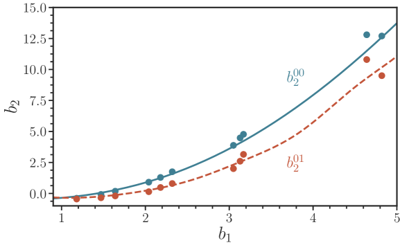
Figure 1: The dependence of the second-order nonlinear effective biases, $b_{2}^{00}$ (blue, solid) and $b_{2}^{01}$ (red, dashed), on the linear bias $b_{1}$ used in this work, as determined from the RunPB simulations. For comparison, the best-fit bias parameters from [54] are shown as circles.

$$b_{s}=-\frac{2}{7}(b_{1}-1).$$ (4.20)

As shown in [54], the tidal bias does not play a prominent role in the biasing model, but nonetheless, we include these terms in our model. The effective biases $b_{2}^{00}$ and $b_{2}^{01}$ have a roughly quadratic dependence on the linear bias $b_{1}$. Rather than freely varying these bias parameters, we treat them as a function of $b_{1}$, independent of redshift, and use simulations to determine the exact functional form of this dependence. We use the set of halo mass bins from the RunPB simulations described in section 2.1 and use Gaussian Process regression (see, e.g., [91]) to predict the functional form of $b_{2}^{00}(b_{1})$ and $b_{2}^{01}(b_{1})$. For this purpose, we use the public Gaussian Process package george [92]. The predictions for $b_{2}^{00}$ and $b_{2}^{01}$ used in this work, as determined from the RunPB simulations, are shown in figure 1. We also show the best-fit bias parameters used in [54] for several redshifts, which are consistent with the results obtained from the RunPB simulations.

4.2.3 Improved modeling of dark matter correlators

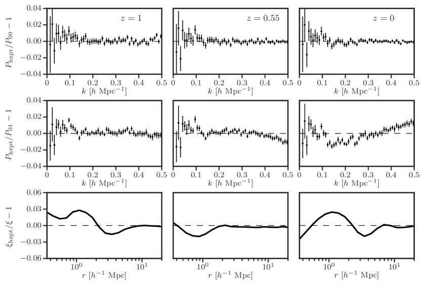
Figure 2: The accuracy of the dark matter HZPT modeling results used in this work, in comparison to the results from the RunPB simulation. We compare the dark matter power spectrum $P_{00}$ (top), density – radial momentum cross-power $P_{01}^{S}$ (middle), and the small-scale correlation function $\xi_{00}$ (bottom). We give results for three redshift outputs: $z=1$ (left), $z=0.55$ (center), and $z=0$ (right). The updated HZPT model parameters are presented in Appendix B.1.

We use the Halo-Zel’dovich Perturbation Theory (HZPT) approach of [59] to model the dark matter density power spectrum $P_{00}(k)$ and the redshift-space cross-correlation of dark matter density and radial momentum $P_{01}^{S}(\mathbf{k})$. This differs from the results presented in [54], which uses standard perturbation theory (SPT) to evaluate these terms (which is known to break down at relatively large scales). Note that the density-momentum cross-correlation can be related to $P_{00}$ through $P_{01}^{S}(\mathbf{k})=\mu^{2}dP_{00}/d\mathrm{ln}a$ [53], so only an accurate model for $P_{00}$ is required. The statistic $P_{01}^{S}(\mathbf{k})$ plays a crucial role in the modeling of the $\mu^{2}$ angular dependence of the redshift-space power spectrum.

The HZPT model connects the Zel’dovich approximation [93, 61] with a Padé expansion for a 1-halo-like term that is determined from simulations using simple, physically motivated parameter scalings. The model for the dark matter power spectrum has been demonstrated to be accurate to 1% to $k\sim 1\ h\text{Mpc}^{-1}$ [59], and the Zel’dovich approximation performs sufficiently well when modeling BAO, relative to other modeling techniques [61, 94].

We provide an update to the HZPT results presented in [59], using the dark matter RunPB simulations detailed in section 2.1. We extend the analysis of [59] to include measurements of $P_{01}^{S}(\mathbf{k})$, as well as the small-scale matter correlation function. We also extend the redshift fitting range, using a set of 10 redshift outputs from the RunPB simulations, ranging from $z=0$ to $z=1$. We perform a global fit of the amplitude and redshift-dependence of the 5 parameters in the HZPT model using the $P_{00}(k)$ and $P_{01}^{S}(\mathbf{k})$ statistics over the range $k=0.005-0.5\ h\text{Mpc}^{-1}$, as well as the small-scale correlation function over the range $r=0.3-25\ \text{Mpc}/h$. Qualitatively, the results remain similar to those presented in [59], but the use of additional statistics (in particular, the small-scale correlation function) in the fit does allow some parameter degeneracies to be broken.

We review the HZPT model for $P_{00}$ and $P_{01}^{S}$ in appendix B.1, and provide the updated best-fit model parameters. We also detail the necessary calculation of $P_{01}^{S}$ in the Zel’dovich approximation in appendix A. We show the accuracy of the HZPT model for the three statistics considered in figure 2 for three redshift snapshots, $z=0$, $0.55$, and $1$. It is evident that the 5-parameter HZPT model can provide a consistent picture of the power spectra to an accuracy of 1-2% over the range of scales considered in this work. Furthermore, keeping in mind that the inclusion of baryonic effects can effect the parameters $R_{1},R_{1h},R_{2h}$ at the 5-10% level [95, 96], the model used in this work performs reasonably well at modeling the notoriously difficult 1-halo to 2-halo regime of the correlation function.

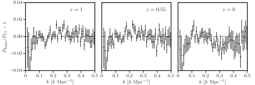
Figure 3: The accuracy of the HZPT model for the auto power spectrum of the dark matter radial momentum $P_{11}^{S}[\mu^{4}]$ in comparison to the results from the RunPB simulations. We give results for three redshift outputs: $z=1$ (left), $z=0.55$ (center), and $z=0$ (right). The best-fit HZPT model parameters are presented in Appendix B.2.

We also extend the HZPT approach to model the dark matter radial momentum auto power spectrum, $P_{11}^{S}(\mathbf{k})$, which is important for modeling the $\mu^{4}$ angular dependence of $P^{S}_{XY,h}(k,\mu)$. Specifically, we model the scalar component of $P_{11}^{S}[\mu^{4}]$ with the sum of a Zel’dovich term and Padé expression and the vector contribution using 1-loop SPT (as was done in [53]). The full model is given by the sum of the scalar and vector contributions

$$P_{11}^{S}[\mu^{4}](k) =P_{11,s}^{S}[\mu^{4}](k)+P_{11,v}^{S}[\mu^{4}](k),$$

$$=P_{11,s}^{\mathrm{zel}}(k)+P^{BB}_{11}(k)-f^{2}I_{31}(k),$$ (4.21)

where the vector contribution $I_{31}(k)$ is defined in [53], and we discuss the Zel’dovich term $P_{11,s}^{\mathrm{zel}}$ in detail in Appendix A. We define the Padé term $P^{BB}_{11}$ and give the best-fit parameters (fit using the RunPB simulations) in Appendix B.2. Figure 3 compares the accuracy of the model in equation 4.21 with the results from the RunPB simulations for three redshift snapshots. The figure shows the model to be accurate to 1-2% over the range of scales of interest.

Finally, rather than using the 1-loop SPT expressions for the dark matter density – velocity divergence cross power spectrum $P_{\delta\theta}(k)$ and the velocity divergence auto power spectrum $P_{\theta\theta}(k)$, we use the fitting formula from [22]. While the 1-loop SPT expressions for $P_{\delta\theta}$ and $P_{\theta\theta}$ diverge from truth at relatively large scales ($k\sim 0.1\ h\text{Mpc}^{-1}$), the model of [22] achieves the necessary accuracy over the range of scales considered in this work.

4.2.4 Halo stochasticity

The $\mu^{0}$ component of the redshift-space halo spectrum, $P^{S}_{XY,h}(k,\mu)$, in the DF model is the isotropic, real-space auto spectrum of the halo density field, $P^{hh}_{00}(k)$. For a complete description of this term, we must accurately model the contribution from the stochasticity of halos, defined for two separate halo mass bins ($h$ and $\bar{h}$) as

$$\Lambda(k)=P_{00}^{h\bar{h}}(k)-\bar{b}_{1}(k)P_{00}^{hm}(k)-b_{1}(k)P_{00}^{\bar{h}m}(k)+b_{1}(k)\bar{b}_{1}(k)P_{00}(k),$$ (4.22)

where $P_{00}^{hm}$ and $P_{00}^{\bar{h}m}$ are the halo–matter cross power spectra for the halo mass bins $h$ and $\bar{h}$, respectively, and $P_{00}$ is the matter power spectrum (modeled using HZPT, as described in section 4.2.3). The scale-dependent linear bias factors are defined as

$$b_{1}(k)\equiv\frac{P^{hm}_{00}(k)}{P_{00}(k)},\ \ \ \ \bar{b}_{1}(k)\equiv\frac{P^{\bar{h}m}_{00}(k)}{P_{00}(k)}.$$ (4.23)

In the Poisson model, the leading-order term of the stochasticity is given by the Poisson shot noise, $\bar{n}^{-1}$, where $\bar{n}$ is the halo number density. However, there are significant deviations from this prediction that have complicated scale dependence. These corrections originate from two competing effects: first, the halo exclusion effects due to the finite size of halos and second, the nonlinear clustering of halos relative to dark matter [86, 54, 97]. In the $k\rightarrow 0$ limit, the stochasticity behaves close to white noise, where halo exclusion lowers the stochasticity relative to the Poisson value and nonlinear clustering leads to a positive contribution. However, in the high-$k$ limit, the stochasticity must approach the Poisson value, and these deviations vanish; thus, there exists a complicated scale dependence that is not well-understood theoretically.

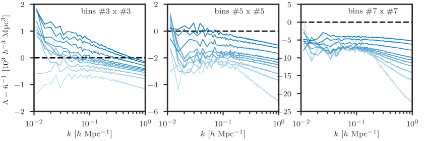
(a) auto halo stochasticity

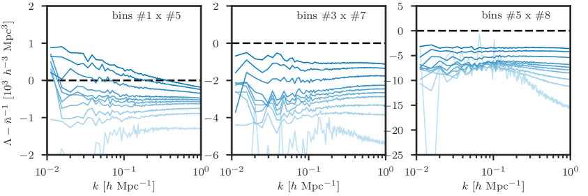
(b) cross halo stochasticity

Figure 4: The deviation of the halo stochasticity $\Lambda(k)$, as defined in equation 4.22, from the Poisson shot noise, for the case of (a) the same halo mass bin and (b) different halo mass bins. Results are measured from the RunPB simulations for three separate combinations of bins. The average halo mass increases from left to right; see Table 2 for halo mass bin details. For each subplot, we show the results for 10 redshifts, ranging from $z=1$ (dark) to $z=0$ (light). Even when the mean halo mass is similar, the scale dependence and amplitude in the cases of auto and cross halo stochasticity can differ significantly.

We use the RunPB simulations at several redshift outputs and the halo mass bins defined in table 2 to investigate the functional form of the halo stochasticity $\Lambda(k)$ as a function of mass and redshift. In figure 4, we show the deviations of the halo stochasticity from the Poisson shot noise when considering the same halo mass bin and different halo mass bins. The trends are consistent with our theoretical understanding: as the average halo mass increases, the stochasticity becomes sub-Poissonian, sourced by halo exclusion effects, while positive contributions from nonlinear biasing become important for lower halo masses. And as halos grow in time, the exclusion effects become more pronounced at lower redshifts [86, 54, 97]. However, the scale dependence and redshift scaling remains non-trivial, and there are significant differences in the scale dependence and amplitude when considering the cases of auto and cross mass bins.

The halo stochasticity was studied in simulations in the context of the DF model in [54], and the results presented here agree with those findings. [54] employs a simple model with log scale dependence to model the auto stochasticity for several mass bins across three redshifts. We extend those results with finer resolution in both redshift and halo mass. In an attempt to capture as much complexity as possible, we treat the halo stochasticity results from the RunPB simulations as a training set and use Gaussian Process regression to predict the auto stochasticity $\Lambda(b_{1},\sigma_{8}(z))$ and cross stochasticity $\Lambda(b_{1},\bar{b}_{1},\sigma_{8}(z))$, where we have parameterized the redshift dependence of the stochasticity using the value of $\sigma_{8}$ at each redshift.

4.2.5 HZPT modeling for the halo-matter cross-correlation

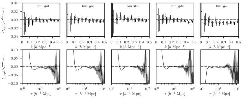
Figure 5: The accuracy of the HZPT model used in this work for the halo-matter cross-correlation, in comparison to the results from the RunPB simulation. We compare the cross power spectrum $P_{hm}$ (top) and the correlation function $\xi^{hm}$ (bottom) for 5 halo mass bins at $z=0.55$ (see table 2 for bin details). We show the measurement uncertainties as error bars for $P^{hm}$ and as the grey shaded region for $\xi^{hm}$. The HZPT parameters have been fit using only $P^{hm}(k)$ from $0.005\ h\text{Mpc}^{-1}<k<0.5\ h\text{Mpc}^{-1}$. The model is a good description of $P^{hm}$ on these scales, as well as $\xi^{hm}$ down to $r\sim 5\ \text{Mpc}/h$, but fails once entering the 1-halo regime on small scales.

The real-space halo-matter cross correlation $P^{hm}(k)$ plays a crucial role in accurately modeling the halo auto spectrum using equation 4.22. We develop a model for the halo-matter power spectrum using HZPT and calibrate the model using the suite of halo mass bins from the RunPB simulations detailed in table 2. To model the Zel’dovich term of the model, we employ a simple, linear bias model, such that the full HZPT model is given by

$$P^{hm}(k)=b_{1}P_{00}^{\mathrm{zel}}(k)+P_{00}^{BB}(k,A_{0},R,R_{1},R_{1h},R_{2h}),$$ (4.24)

where $b_{1}$ is the large-scale, linear bias of the halo field, $P_{00}^{\mathrm{zel}}$ is the matter density auto spectrum in the Zel’dovich approximation, and $P_{00}^{BB}$ is a broadband Padé term, as given by equation B.1. To fully account for the biased nature of the halo field, the HZPT model parameters, $\{A_{0},R,R_{1},R_{1h},R_{2h}\}$, now become a function of not only $\sigma_{8}(z)$ but also the linear bias $b_{1}$. We choose a simple power-law functional form for the $b_{1}$ dependence, which performs well at modeling the bias dependence of $P^{hm}$ over the range of scales of interest in this work. We perform a global fit across the 8 halo mass bins and 10 redshifts of the RunPB simulations to determine the best-fit HZPT model parameters. In our parameter fit, we have included the cross power spectrum $P^{hm}$ on scales ranging from $k=0.005\ h\text{Mpc}^{-1}$ to $k=0.5\ h\text{Mpc}^{-1}$. The best-fit parameters are presented in appendix B.3.

We show the accuracy of the halo-matter HZPT model in figure 5 for several halo mass bins at $z=0.55$. The trends evident at this redshift are consistent with the results from the full range of redshifts explored ($z=0-1$). The model reproduces the cross power spectrum $P^{hm}$ at the $\sim$2% level, as well as the cross-correlation $\xi^{hm}$ on scales $r\gtrsim 5$ Mpc/$h$. However, we see from the correlation function results on small scales that the model is unable to reproduce the clustering on scales within the 1-halo regime, where halo profile details become important. The model breakdown on these scales is due to the choice to use a power-law dependence on $b_{1}$ for the HZPT parameters that are related to the halo profile. To better describe halo profiles and capture the effects of nonlinear and nonlocal bias terms, i.e., [87], a more complicated functional form for the linear bias dependence is required. However, because Fourier-space statistics are the main concern of this work and the simplified model performs well when modeling the power spectrum on the scales of interest, we leave the investigation of improved small-scale modeling to future work.

4.3 Modeling observational effects

In this section we discuss several details that arise when modeling data from real galaxy surveys. In section 4.3.1, we describe how we account for the geometric distortions that occur when an inaccurate fiducial cosmology is assumed due to the AP effect. Section 4.3.2 discusses how we treat the survey geometry and window function when modeling realistic “cutsky” mocks, which have a realistic survey geometry imposed.

4.3.1 The Alcock-Paczynski effect

When analyzing data from galaxy surveys, we must transform observed angular positions and redshifts into physical coordinates, using a fiducial cosmological model to specify the relation between the redshift and the LOS distance (i.e., the Hubble parameter) and between the angular separation and the distance perpendicular to the LOS (i.e., the angular diameter distance). If the fiducial cosmology differs from the true cosmology, an anisotropic, geometric warping of the clustering signal is introduced. This distortion, known as the Alcock- Paczynski (AP) effect, [13] is distinct from RSD and can be used to measure cosmological parameters. The presence of the BAO feature at a fixed scale in the power spectrum helps distinguish the geometric AP effect and the dynamical RSD anisotropy, thus increasing the constraining power of full-shape modeling [12, 98].

The difference between the assumed and true cosmological models results in a rescaling of the wavenumbers transverse $k_{\perp}$ and parallel $k_{\parallel}$ to the LOS direction, such that

$$k^{\prime}_{\perp}=q_{\perp}k_{\perp}\ \mathrm{and}\ k^{\prime}_{\parallel}=q_{\parallel}k_{\parallel},$$ (4.25)

where the primes denote quantities that are observed assuming the fiducial (and possibly incorrect) cosmology. The two distortion parameters $q_{\perp}$ and $q_{\parallel}$ are given by

$$q_{\perp}=\frac{D_{A}(z_{\mathrm{eff}})}{D^{\prime}_{A}(z_{\mathrm{eff}})}\ \mathrm{and}\ q_{\parallel}=\frac{H^{\prime}(z_{\mathrm{eff}})}{H(z_{\mathrm{eff}})},$$ (4.26)

which are the ratios of the Hubble parameter and angular diameter distance in the fiducial and true cosmologies at the effective redshift of the survey. With these definitions, the theoretical prediction for the multipole power spectrum when including the AP effect can be expressed as

$$P_{\ell}(k^{\prime})=\frac{2\ell+1}{2q_{\perp}q_{\parallel}^{2}}\int_{-1}^{1}d\mu\ P^{S}_{gg}\left[k(k^{\prime},\mu^{\prime}),\mu(\mu^{\prime})\right]\mathcal{L}_{\ell}(\mu),$$ (4.27)

where $\mathcal{L}_{\ell}$ is the Legendre polynomial of order $\ell$, and we use the model prediction of equation 4.5 for $P^{S}_{gg}[k^{\prime}(k,\mu),\mu(\mu^{\prime})]$. The true $(k,\mu)$ can be related to the observed $(k^{\prime},\mu^{\prime})$ via

$$k(k^{\prime},\mu^{\prime}) =\frac{k^{\prime}}{q_{\perp}}\left[1+(\mu^{\prime})^{2}\left(\frac{1}{F^{2}}-1\right)\right]^{1/2},$$ (4.28)

$$\mu(\mu^{\prime}) =\frac{\mu^{\prime}}{F}\left[1+(\mu^{\prime})^{2}\left(\frac{1}{F^{2}}-1\right),\right]^{-1/2}$$ (4.29)

where $F=q_{\parallel}/q_{\perp}$. The normalization scaling of the power spectrum with $q_{\perp}^{-1}q_{\parallel}^{-2}$ is due to the volume distortion between the two different cosmologies.

For comparison with BAO distance analyses, a second set of AP parameters is usually defined, given by

$$\alpha_{\perp} \equiv\frac{D_{A}(z_{\mathrm{eff}})}{D^{\prime}_{A}(z_{\mathrm{eff}})}\frac{r_{d}^{\prime}}{r_{d}}=q_{\perp}\frac{r_{d}^{\prime}}{r_{d}}$$ (4.30)

$$\alpha_{\parallel} \equiv\frac{H^{\prime}(z_{\mathrm{eff}})}{H(z_{\mathrm{eff}})}\frac{r_{d}^{\prime}}{r_{d}}=q_{\parallel}\frac{r_{d}^{\prime}}{r_{d}},$$ (4.31)

where we have defined $r_{d}\equiv r_{s}(z_{d})$ as the sound horizon scale at the drag redshift $z_{d}$. BAO measurements are sensitive to the Hubble parameter and angular diameter distance relative to the sound horizon scale of a fixed “template” cosmology, and this second set of parameter definitions facilitates comparison of measurements using different template cosmological models.

4.3.2 The survey geometry

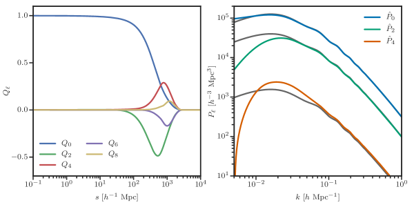
Figure 6: The window function multipoles in configuration space (left) and the effects of the window function on linear Kaiser power spectrum multipoles (right) for the DR12 CMASS NGC survey geometry. In the right panel, the solid grey lines show the unconvoled multipoles, while the colored lines correspond to the model after convolution with the window function, $\hat{P}_{\ell}(k)$. The convolution procedure has large effects at small $k$, and we choose to use $k_{\mathrm{min}}=0.02\ h\text{Mpc}^{-1}$ in our data analysis to minimize these effects.

When analyzing cutsky mock catalogs, we must account for the effects of the survey geometry when comparing our theoretical model to the measured power spectrum. We do this by convolving our theoretical model with the survey window function, rather than trying to remove the effect of the survey geometry from the data itself. Our window function treatment follows the method first presented in [99] and used in the analysis of BOSS DR12 data in [39, 100].

Following [99], we compute the window function multipoles in configuration space using a pair counting algorithm and the catalog of random objects describing the survey geometry. We use the Corrfunc correlation function code [101] to compute the pair counts of the random catalog via

$$Q_{\ell}(s)\propto\int_{-1}^{1}d\mu RR(s,\mu)\mathcal{L}_{\ell}(\mu)\simeq\sum_{i}RR(s_{i},\mu_{i})\mathcal{L}_{\ell}(\mu_{i}),$$ (4.32)

where the normalization is such that $Q_{0}(s)\rightarrow 1$ for $s\ll 1$. The resulting multipoles $Q_{\ell}$ for the BOSS CMASS NGC sample are shown in the left panel of figure 6. The $Q_{\ell}$ vanish for scales $\gtrsim 3000\ \ h^{-1}\text{Mpc}$, as these are the largest scales in the volume of the NGC. Note that on small scales, the clustering becomes isotropic, with the multipoles vanishing. In general, the contribution of the higher-order multipoles decreases as $\ell$ increases, which guarantees the convolution converges when including only the first few $Q_{\ell}$. Here, we include results up to and including $Q_{8}$, and have verified that the inclusion of $Q_{10}$ does not affect our results.

With the measured $Q_{\ell}$, we compute the convolved theoretical correlation function multipoles in configuration space as

$$\hat{\xi}_{0}(s)=\xi_{0}Q_{0} +\frac{1}{5}\xi_{2}Q_{2}+\frac{1}{9}\xi_{4}Q_{4}+...$$

$$\hat{\xi}_{2}(s)=\xi_{0}Q_{2} +\xi_{2}\left[Q_{0}+\frac{2}{7}Q_{2}+\frac{2}{7}Q_{4}\right]$$

$$+\xi_{4}\left[\frac{2}{7}Q_{2}\frac{100}{693}Q_{4}+\frac{25}{143}Q_{6}\right]+...$$

$$\hat{\xi}_{4}(s)=\xi_{0}Q_{4} +\xi_{2}\left[\frac{18}{35}Q_{2}+\frac{20}{77}Q_{4}+\frac{45}{143}Q_{6}\right]$$

$$+\xi_{4}\left[Q_{0}+\frac{20}{77}Q_{2}+\frac{162}{1001}Q_{4}+\frac{20}{143}Q_{6}+\frac{490}{2431}Q_{8}\right]+....,$$ (4.33)

where $\xi_{\ell}$ are the theoretical correlation function mutipoles, computed from the power spectrum multipoles via a 1D Hankel transform, evaluated using the FFTLog software [102]. We also perform the transformation from $\hat{\xi}_{\ell}(s)$ to $\hat{P}_{\ell}(k)$ using FFTLog.

The effects of the window function convolution can be seen in the right panel of figure 6, where we illustrate the effects using linear Kaiser multipoles. The effects are most important on scales of order the survey size; for the NGC CMASS sample, the window function effects are only important on scales $k\lesssim 0.05\ h\text{Mpc}^{-1}$. The impact of the survey geometry increases for the higher-order multipoles, with the anisotropy of the window function leading to non-trivial effects on our convolved model. In this work, we use a minimum wavenumber of $k_{\mathrm{min}}=0.02\ h\text{Mpc}^{-1}$ when comparing data and theory and have tested that the window function convolution has minimal impact on our parameter fitting analyses. However, as measurement errors decrease for future surveys, the window convolution will need to be carefully tested, given both the constraining power of the $\ell=2$ and $4$ multipoles and the larger convolution effects.

4.4 Model parametrization

Free Parameters
Name [Unit]	Prior
$\alpha_{\perp}$	$\mathcal{U}(0.8,1.2)$
$\alpha_{\parallel}$	$\mathcal{U}(0.8,1.2)$
$f$	$\mathcal{U}(0.6,1.0)$
$\sigma_{8}(z_{\mathrm{eff}})$	$\mathcal{U}(0.3,0.9)$
$b_{1,c_{A}}$	$\mathcal{U}(1.2,2.5)$
$f_{s}$	$\mathcal{U}(0,0.25)$
$f_{s_{B}}$	$\mathcal{U}(0,1)$
$\left\langle N_{>1,s}\right\rangle$	$\mathcal{N}(2.4,0.1)$
$\sigma_{c}$ [$\ h^{-1}\text{Mpc}$]	$\mathcal{U}(0,3)$
$\sigma_{s_{A}}$ [$\ h^{-1}\text{Mpc}$]	$\mathcal{U}(2,6)$
$\gamma_{s_{A}}$	$\mathcal{N}(1.45,0.3)$
$\gamma_{s_{B}}$	$\mathcal{N}(2.05,0.3)$
$f^{1h}_{s_{B}s_{B}}$	$\mathcal{N}(4,1)$

Constrained Parameters
Name [Unit]	Constraint Expression
$b_{1,c_{B}}$	equation C.7
$b_{1,s_{A}}$	$\gamma_{s_{A}}b_{1,c_{A}}$
$b_{1,s_{B}}$	$\gamma_{s_{B}}b_{1,c_{A}}$
$f_{c_{B}}$	equation C.2
$\sigma_{s_{B}}$ [$h^{-1}$ Mpc]	$\sigma_{s_{A}}\left[\sigma_{v}^{\mathrm{model}}(b_{1,s_{B}})/\sigma_{v}^{\mathrm{model}}(b_{1,s_{A}})\right]$
$N_{c_{B}s}$ [$h^{-3}\ \mathrm{Mpc}^{3}$]	equation C.12
$N_{s_{B}s_{B}}$ [$h^{-3}\ \mathrm{Mpc}^{3}$]	equation C.16

Table 3: The parameter space of our full-shape RSD fits using the model described in this work. There are 13 free parameters (left) that are varied during the fitting process, with several additional parameters subject to constraint expressions (right). For all free parameters, we provide the prior used when fitting, either a normal prior $\mathcal{N}(\mu,\sigma)$ with mean $\mu$ and standard deviation $\sigma$, or a uniform prior $\mathcal{U}(a,b)$ with lower bound $a$ and upper bound $b$. For a detailed description of the model parameters, see section 4.4.

Table 3 gives a summary of the parameters of the model described in this work. We give both the free parameters as well as the constrained parameters and the corresponding constraint expressions. There are 13 free parameters detailed in table 3, and these parameters correspond to the parameter space used in our RSD analyses. The table also lists the assumed prior distribution for each parameter used during parameter estimation, which is either a flat (uniform) or Gaussian prior. We use physically motivated priors when possible and assume wide, flat priors on all cosmological parameters of interest. We describe the model parametrization in detail below.

4.4.1 Cosmology parameters

The free parameters specifying the cosmology in our model are the AP distortion parameters ($\alpha_{\parallel}$ and $\alpha_{\perp}$), the growth rate $f$, and the amplitude of matter fluctuations $\sigma_{8}$, where both $f$ and $\sigma_{8}$ are evaluated at the effective redshift of the sample, $z_{\mathrm{eff}}$. During our fitting procedure, we vary $f$ and $\sigma_{8}$ independently, although we only report results for the product $f\sigma_{8}$, which is the parameter combination most well-constrained by RSD analyses. The model requires a linear power spectrum in order to evaluate several perturbation theory integrals. These integrals are computationally costly (although see recent advances, [103, 104, 105]), and for this reason, we do not vary any cosmological parameters affecting the shape of the linear power spectrum during parameter estimation. We evaluate the linear power spectrum using the fiducial cosmology and keep the shape fixed, allowing only the amplitude to vary through changes in $\sigma_{8}$.

4.4.2 Linear bias parameters

In the most general version of the model discussed in section 4.1, we must specify linear bias parameters for each of the four galaxy subsamples: $b_{1,c_{A}}$, $b_{1,c_{B}}$, $b_{1,s_{A}}$, and $b_{1,s_{B}}$. As discussed in section 4.2.2, the linear bias fully predicts the higher-order biasing parameters for a given sample. When varying the linear bias parameters of the $s_{A}$ and $s_{B}$ satellite samples, we enforce the expected ordering of the parameters: $b_{1,c_{A}}<b_{1,s_{A}}<b_{1,s_{B}}$. We use the relations $b_{1,s_{A}}=\gamma_{s_{A}}b_{1,c_{A}}$ and $b_{1,s_{B}}=\gamma_{s_{B}}b_{1,c_{A}}$ and choose to vary the parameters $\gamma_{s_{A}}$ and $\gamma_{s_{B}}$ instead. We use relatively wide Gaussian priors for these parameters centered on their expected fiducial values for a CMASS-like galaxy sample, $\gamma_{s_{A}}\sim 1.45$ and $\gamma_{s_{B}}\sim 2.05$. For the linear bias of the $c_{B}$ sample, we use the expected scaling of the bias with the biases of the satellite samples as given by equation C.7 and described in appendix C.2.

4.4.3 Sample fractions, velocity dispersions, and 1-halo amplitudes

There are three parameters specifying the fraction of all galaxies that are satellites $f_{s}$, the fraction of centrals that live in halos with a satellite $f_{c_{B}}$, and the fraction of satellites that live in halos with multiple satellites $f_{s_{B}}$. We must also specify the 1-halo amplitudes (assumed to be independent of $k$) that enter into equations 4.14 - 4.16. We denote the 1-halo amplitude due to correlations between centrals and satellites in the same halo as $N_{c_{B}s}$, and between satellites inside the same halo as $N_{s_{B}s_{B}}$. And, finally, we must specify the velocity dispersion parameters for each galaxy subsample in order to account for the FoG effect. We include a single velocity dispersion for centrals, $\sigma_{c}$, and parameters for each of the satellite subsamples, $\sigma_{s_{A}}$ and $\sigma_{s_{B}}$. Thus, in the most general case, there are additional 12 model parameters needed to fully evaluate our model, in addition to the 4 cosmological parameters.

There are dependencies between the parameters previously discussed that allow us to parametrize the model in terms of alternative parameters that have well-behaved, physically motivated priors. In particular, we use the constraints outlined in appendix C for the relative fraction of the $c_{B}$ sample, $f_{c_{B}}$, in equation C.2, and for the 1-halo amplitudes, $N_{c_{B}s}$ and $N_{c_{B}c_{B}}$, in equations C.12 and C.16. In the former case, the constraint allows us to vary the parameter $\left\langle N_{>1,s}\right\rangle$, which is defined as the mean number of satellite galaxies in halos with more than one satellite. This parameter is typically centered on $\left\langle N_{>1,s}\right\rangle\sim 2.4$ for CMASS-like galaxy samples, with little variation around this center value. For the 1-halo amplitude $N_{s_{B}s_{B}}$ we vary a normalization parameter $f^{1h}_{s_{B}s_{B}}$ to account for uncertainty in the expected value, which should have a value of order unity.

Finally, we do not vary the velocity dispersion of the $s_{B}$ sample, $\sigma_{s_{B}}$, but rather use the physically motivated scaling with halo mass, $\sigma_{v}^{2}\propto M^{2/3}$, and the halo bias – mass relation from [106]. We do not use this model function $\sigma_{v}^{\mathrm{model}}(b_{1})$ to predict the absolute amplitude of $\sigma_{s_{B}}$, but only the functional form. We always rescale the predicted value by the current value of $\sigma_{s_{A}}$ (see table 3 for details).

5 Performance of the model

5.1 RunPB results

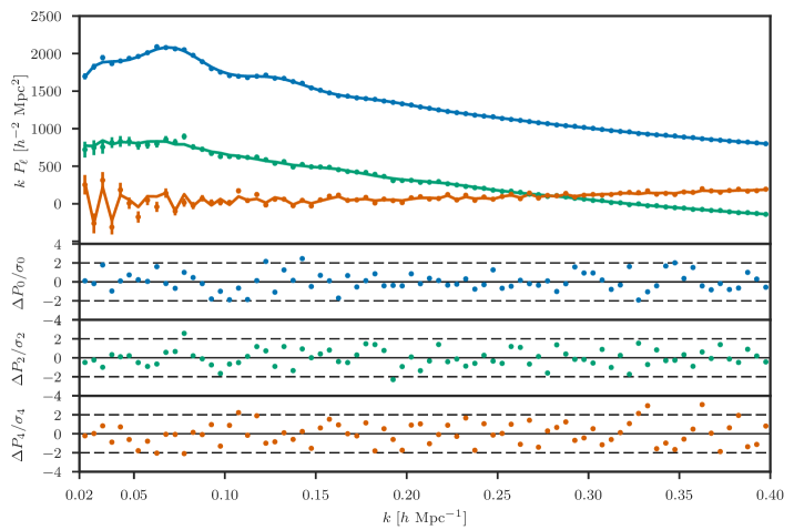
Figure 7: The best-fit monopole, quadrupole, and hexadecapole models (lines) as compared to the measurements (points) from the mean of 10 RunPB HOD galaxy realizations at $z=0.55$, fit over the wavenumber range $k=0.02-0.4\ h\text{Mpc}^{-1}$. The lower panels show the model residuals for each multipole separately. The reduced chi-squared of the fit to all three multipoles is $\chi^{2}_{\mathrm{red}}=1.12$. Note that the large variation from bin to bin in the hexadecapole is due to discrete binning effects.

As a first test of the RSD model described in section 4, we use a set of HOD galaxy catalogs constructed from 10 realizations of the $z=0.55$ snapshot of the RunPB simulation, described previously in section 2.1. The galaxy catalogs are made by populating halo catalogs according to a halo occupation distribution with parameters comparable to the BOSS CMASS sample. The halo catalogs are constructed in the manner described in detail in [36]. Briefly, the halo finder uses the spherical overdensity implementation of [107], using an overdensity of $\Delta_{m}=200$ relative to the mean matter density $\rho_{m}$ to define the halo virial radius. Central galaxies are not at rest with respect to the halo center-of-mass; they are assigned a velocity computed from the halo particles in the densest region of each halo (see [36] for details). Note that the halo catalogs used here are not the same as the FOF halo catalogs described in section 2.1, which we use to calibrate certain components of the RSD model. Differences in the halo finder algorithms lead to important differences in the clustering of the resulting galaxy catalogs. While we do not expect RSD fits to these galaxy catalogs to be a fully-independent validation of the model, they do still provide a useful test of the accuracy of our model.

Using the model parameterization discussed in section 4.4, we fit the mean of the measured monopole, quadrupole, and hexadecapole from 10 realizations at $z=0.55$ as a function of the maximum wavenumber included in the fits, $k_{\mathrm{max}}=[0.2,0.3,0.4]\ h\text{Mpc}^{-1}$. The resulting best-fit model and residuals between measurements and theory are shown in figure 7 for $k_{\mathrm{max}}=0.4\ h\text{Mpc}^{-1}$. We are able to achieve excellent agreement between the model and simulation multipoles to scales of $k=0.4\ h\text{Mpc}^{-1}$, well into the nonlinear clustering regime.

As a function of $k_{\mathrm{max}}$, we report the mean and $1\sigma$ error for a subset of the model parameters in table 4, as determined from the posterior distributions obtained via MCMC sampling. We also show the 2D posterior distributions for $f\sigma_{8}$, $\alpha_{\parallel}$, and $\alpha_{\perp}$ for each $k_{\mathrm{max}}$ value in figure 8. As expected, we obtain significant decreases in parameter uncertainties when including small-scale information in the fits. For the three cosmology parameters, $f\sigma_{8}$, $\alpha_{\parallel}$, and $\alpha_{\perp}$, we find decreases of 19%, 18%, and 18%, respectively, for $k_{\mathrm{max}}=0.3\ h\text{Mpc}^{-1}$ and 38%, 24%, and 29% for $k_{\mathrm{max}}=0.4\ h\text{Mpc}^{-1}$, relative to the fit using $k_{\mathrm{max}}=0.2\ h\text{Mpc}^{-1}$. These decreases are roughly consistent with the expected scaling in the nonlinear regime, $\sigma\propto k_{\mathrm{max}}^{-1/2}$ (e.g., [55]). For the AP parameters, we find more modest decreases in the uncertainty when ranging from $k_{\mathrm{max}}=0.2\ h\text{Mpc}^{-1}$ to $k_{\mathrm{max}}=0.4\ h\text{Mpc}^{-1}$. In particular, extending from $k_{\mathrm{max}}=0.3\ h\text{Mpc}^{-1}$ to $k_{\mathrm{max}}=0.4\ h\text{Mpc}^{-1}$ offers little improvement in the error on $\alpha_{\parallel}$. The constraining power for the AP parameters results from a combination of the BAO signal and information from the geometric distortion of the full broadband signal. As nearly all of the information from the BAO signal is present below $k=0.2\ h\text{Mpc}^{-1}$, our more modest decreases in uncertainty for the AP parameters are consistent with our expectations.

We have central/satellite information for each galaxy in the RunPB catalogs and can assess the accuracy of the halo model decomposition described in section 4.1. As seen in table 4, we find a non-zero velocity dispersion for centrals with an amplitude $\sigma_{c}\sim 1\ h^{-1}\text{Mpc}$, which is consistent with the expected amplitude present in the underlying halo catalogs. The main discrepancy is that our recovered satellite fraction is significantly higher than the expected value. This results from the fact that we rely on FOF halo catalogs for calibration of the halo clustering in the model, while we are fitting galaxy catalogs created from SO catalogs. The choice of halo finder alters the clustering on scales around the virial radius. A FOF halo finder tends to over-merge halos on these scales into a single halo, whereas a SO finder tends to preserve the multiple smaller halos. This effect manifests itself as an increase in the model satellite fraction and is consistent with our fitting results. Thus, we are able to absorb issues related to these simulation differences into the satellite fraction parameter.

	$k_{\mathrm{max}}=0.2$ $h/\mathrm{Mpc}$	$k_{\mathrm{max}}=0.3$ $h/\mathrm{Mpc}$	$k_{\mathrm{max}}=0.4$ $h/\mathrm{Mpc}$	truth
$f\sigma_{8}$	$0.454\,635\,3$ ${}^{$0.014\,874\,61$}_{$-0.015\,375\,89$}$	$0.467\,202\,4$ ${}^{$0.012\,208\,06$}_{$-0.012\,776\,18$}$	$0.468\,914\,2$ ${}^{$0.009\,673\,357$}_{$-0.009\,075\,522$}$	$0.472$
$f\sigma_{8}$ [fixed AP]	$0.456\,554\,949\,284$ ${}^{$0.009\,506\,178\,859\,96$}_{$-0.009\,782\,582\,521\,44$}$	$0.465\,566\,307\,306$ ${}^{$0.008\,551\,955\,223\,08$}_{$-0.008\,344\,471\,454\,62$}$	$0.467\,769\,473\,791$ ${}^{$0.006\,899\,029\,016\,49$}_{$-0.007\,103\,681\,564\,33$}$	$0.472$
$\alpha_{\perp}$	$1.002\,88$ ${}^{$0.005\,369\,816$}_{$-0.006\,284\,306$}$	$1.004\,21$ ${}^{$0.004\,924\,848$}_{$-0.004\,572\,193$}$	$1.004\,951$ ${}^{$0.004\,241\,419$}_{$-0.004\,049\,029$}$	$1.0$
$\alpha_{\parallel}$	$1.008\,968$ ${}^{$0.009\,548\,766$}_{$-0.008\,575\,451$}$	$1.006\,492$ ${}^{$0.007\,784\,377$}_{$-0.007\,363\,477$}$	$1.008\,892$ ${}^{$0.006\,819\,668$}_{$-0.007\,680\,713$}$	$1.0$
$b_{1}\sigma_{8}$	$1.265\,523$ ${}^{$0.008\,938\,074$}_{$-0.008\,676\,291$}$	$1.264\,623$ ${}^{$0.007\,589\,221$}_{$-0.008\,247\,495$}$	$1.2681$ ${}^{$0.007\,574\,999$}_{$-0.008\,005\,503$}$	$1.272$
$f_{s}$	$0.121\,926$ ${}^{$0.018\,844\,78$}_{$-0.018\,429\,13$}$	$0.142\,780\,5$ ${}^{$0.012\,625\,22$}_{$-0.013\,169\,97$}$	$0.143\,392\,6$ ${}^{$0.007\,552\,902$}_{$-0.008\,046\,28$}$	$0.104$
$f_{c_{B}}$	$0.104\,029\,6$ ${}^{$0.033\,389\,25$}_{$-0.029\,778\,29$}$	$0.123\,522\,7$ ${}^{$0.022\,464\,64$}_{$-0.023\,447\,92$}$	$0.121\,998\,4$ ${}^{$0.013\,359\,13$}_{$-0.014\,904\,8$}$	$0.089$
$f_{s_{B}}$	$0.437\,855$ ${}^{$0.203\,009\,2$}_{$-0.197\,398\,2$}$	$0.437\,761\,3$ ${}^{$0.136\,482\,5$}_{$-0.123\,428\,9$}$	$0.466\,220\,9$ ${}^{$0.081\,457\,78$}_{$-0.079\,203\,44$}$	$0.399$
$\sigma_{c}$	$1.133\,505$ ${}^{$0.214\,393\,7$}_{$-0.238\,313\,2$}$	$0.906\,037\,8$ ${}^{$0.088\,157\,92$}_{$-0.111\,175\,9$}$	$0.929\,731\,3$ ${}^{$0.062\,050\,01$}_{$-0.064\,733\,97$}$	–
$\sigma_{s_{A}}$	$4.239\,433$ ${}^{$0.475\,533\,5$}_{$-0.412\,556\,1$}$	$3.737\,315$ ${}^{$0.372\,063\,4$}_{$-0.464\,384\,7$}$	$3.443\,024$ ${}^{$0.277\,893\,1$}_{$-0.270\,151\,9$}$	–
$\chi^{2}$/d.o.f.	$113/(108-13)=1.19$	$159/(168-13)=1.03$	$241/(228-13)=1.12$

Table 4: Parameter constraints obtained when fitting the 13-parameter RSD model to $[P_{0},P_{2},P_{4}]$, as measured from the mean of the 10 RunPB galaxy catalogs at $z=0.55$. We show results determined as a function of the maximum wavenumber included in the fits. Parameter posteriors are determined from MCMC sampling of the likelihood, assuming Gaussian covariance between multipoles.

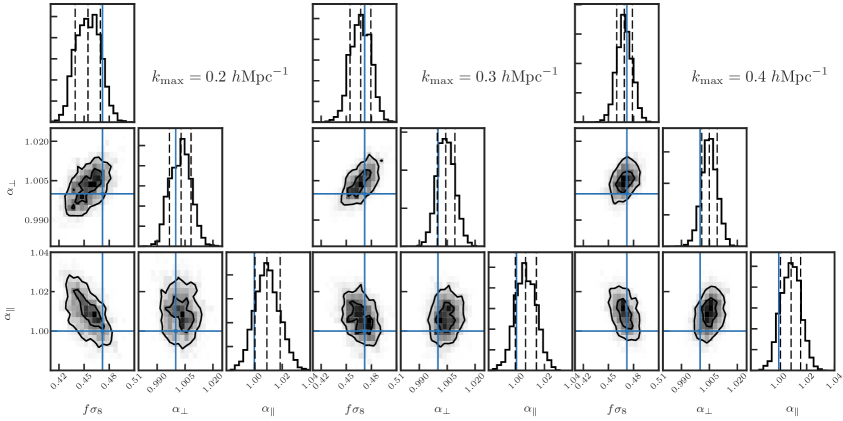
Figure 8: The 2D posterior distributions for the cosmology parameters $f\sigma_{8}$, $q_{\parallel}$, and $q_{\perp}$ obtained from fitting the mean of 10 RunPB HOD galaxy realizations at $z=0.55$. We show results when varying the maximum scale included in the fits: $k_{\mathrm{max}}=0.2$ (left), 0.3 (center), 0.4 (right)$\ h\text{Mpc}^{-1}$. The expected parameter values are marked with solid blue lines.

We analyze the correlations between the posterior distributions to better understand the constraining power of our 13-parameter model. We show these parameter correlations for each fitting range in figure 9. As expected, we find that the main parameter combination measuring the strength of RSD $f\sigma_{8}$ is most correlated with the AP parameters $\alpha_{\parallel}$ and $\alpha_{\perp}$, which measure geometric distortions of the clustering signal. For each of the $k_{\mathrm{max}}$ fitting ranges, the correlation matrix for ($f\sigma_{8},\alpha_{\perp},\alpha_{\parallel}$) is:

$$R^{0.2}[f\sigma_{8},\alpha_{\perp},\alpha_{\parallel}] =\begin{bmatrix}[r]1.000&0.536&-0.583\\ 0.536&1.000&-0.094\\ -0.583&-0.094&1.000\end{bmatrix},$$ (5.1)

$$R^{0.3}[f\sigma_{8},\alpha_{\perp},\alpha_{\parallel}] =\begin{bmatrix}[r]1.000&0.605&-0.361\\ 0.605&1.000&0.133\\ -0.361&0.133&1.000\\ \end{bmatrix},$$ (5.2)

$$R^{0.4}[f\sigma_{8},\alpha_{\perp},\alpha_{\parallel}] =\begin{bmatrix}[r]1.000&0.377&-0.418\\ 0.377&1.000&0.292\\ -0.418&0.292&1.000\\ \end{bmatrix}.$$ (5.3)

As we extend the maximum wavenumber included in our fits, small-scale information does help break degeneracies between $f\sigma_{8}$ and the AP parameters, reducing the correlation between $f\sigma_{8}$ and ($\alpha_{\perp}$, $\alpha_{\parallel}$). For comparison, [39] reports a correlation between $f\sigma_{8}$ and $\alpha_{\perp}$ of 0.503 and $f\sigma_{8}$ and $\alpha_{\parallel}$ of 0.547 for the middle redshift bin for the combined DR12 BOSS sample, where they have fit [$P_{0}$, $P_{2}$] to $k_{\mathrm{max}}=0.15\ h\text{Mpc}^{-1}$ and $P_{4}$ to $k_{\mathrm{max}}=0.1\ h\text{Mpc}^{-1}$. This level of correlation is similar to our values obtained when fitting to $k_{\mathrm{max}}=0.2\ h\text{Mpc}^{-1}$, however we find a significant reduction in correlation fitting to $k_{\mathrm{max}}=0.4\ h\text{Mpc}^{-1}$. We can assess the freedom of our RSD modeling using the Fisher formalism, which predicts a correlation coefficient of unity between $\alpha_{\parallel}$ and $\alpha_{\perp}$ in the case where we perfectly understand RSD [108, 109, 12]. In the opposite limit, we expect $r\sim-0.4$ when only BAO information is used and RSD information is fully marginalized over. Thus, the correlation between $\alpha_{\parallel}$ and $\alpha_{\perp}$ provides a measure of the constraining power of our RSD parametrization, with the correlation decreasing from unity as additional freedom is introduced into the RSD model. Our results are consistent with this expectation, as we find the correlation increase for large $k_{\mathrm{max}}$. To model results only to $k_{\mathrm{max}}=0.2\ h\text{Mpc}^{-1}$, our model contains too much freedom, in comparison to the requirements of modeling to $k_{\mathrm{max}}=0.4\ h\text{Mpc}^{-1}$. Again for comparison, [39] finds a correlation of $r=0.257$ between $\alpha_{\parallel}$ and $\alpha_{\perp}$. Thus, our value of $r=0.292$ indicates that we are able to recover a similar amount of information using our RSD model parametrization to $k_{\mathrm{max}}=0.4\ h\text{Mpc}^{-1}$.

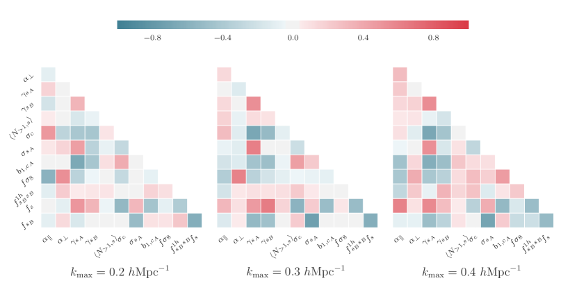
Figure 9: Parameter correlations as measured from the posterior distributions when fitting the mean of the 10 RunPB galaxy catalogs. We show the correlations as a function of the maximum wavenumber included in the fit, illustrating the changes in parameter dependencies when fitting to smaller scales.

5.2 Independent tests on high resolution mocks

To fully assess the accuracy and precision of our RSD model, we perform independent tests using two sets of mocks based on high-fidelity, periodic $N$-body simulations. The first, described in §5.2.1 is a homogenenous set of 21 galaxy catalogs derived from 7 realizations of a $N$-body simulation with fixed cosmology and bias model. The second, described in §5.2.2, is a set of 7 heterogenous HOD galaxy catalogs where both the bias model and underlying cosmology varies from box to box. For details on the cosmology and simulation parameters for these mocks, see table 1.

5.2.1 Cubic N-series results

Figure 10: The mean of the best-fit monopole, quadrupole, and hexadecapole models (colored) as compared to the individual measurements (gray) from the 21 N-series cubic boxes at $z=0.5$, fit over the wavenumber range $k=0.02-0.4\ h\text{Mpc}^{-1}$. The lower panels show the scatter in the recovered values for the 3 cosmology parameters, $f\sigma_{8}$, $\alpha_{\perp}$, and $\alpha_{\parallel}$, across the 21 boxes. The error bar shows the standard deviation of these results (not the error on the mean).

Our first independent tests utilize the cubic N-series simulation, the large-volume ($L_{\mathrm{box}}=2600\ h^{-1}\text{Mpc}$) periodic box simulations described in section 2.2. We perform fits to the monopole, quadrupole, and hexadecapole from 21 HOD galaxy catalogs, constructed from 7 realizations at $z=0.5$ and 3 orthogonal line-of-sight projections per box. The cosmology of these boxes is given in table 1. As in section 5.1, we perform fits to the data vector [$P_{0},P_{2},P_{4}$] over a range of $k_{\mathrm{max}}$ values. The best-fitting parameters for each of the 21 catalogs are obtained by maximum a posterior (MAP) estimation using the LBFGS algorithm.

Figure 10 shows the measured $\ell=0$, $2$, and $4$ multipoles from the individual N-series catalogs, and we have over-plotted the mean of the best-fitting model from each fit using $k_{\mathrm{max}}=0.4\ h\text{Mpc}^{-1}$. We report the mean (with the expected value subtracted) and standard deviation for the best-fitting $f\sigma_{8}$, $\alpha_{\perp}$, and $\alpha_{\parallel}$ values from the 21 fits as a function of fitting range in table 5. We also include the results for $f\sigma_{8}$ when holding the AP parameters fixed to their true values.

We find similar trends in our recovered cosmological parameters for the N-series boxes as for the RunPB results in §5.1. We obtain good fits to the measured $\ell=0,2,4$ multipoles using our RSD model up to $k_{\mathrm{max}}=0.4\ h\text{Mpc}^{-1}$. However, we do find some evidence for small systematic biases present in our RSD model, although it is difficult to properly assess the level of statistical significance with only seven fully independent realizations (clustering from boxes that vary only the line-of-sight projection are correlated). When using $k_{\mathrm{max}}=0.4\ h\text{Mpc}^{-1}$, we find that are $f\sigma_{8}$ value is biased low by $\Delta f\sigma_{8}$ = 0.008 and $\alpha_{\parallel}$ is biased high by $\Delta\alpha_{\parallel}=0.011$. These correspond to $\sim$$0.8\sigma$ and $\sim$$0.9\sigma$ shifts, respectively, relative to the box-to-box dispersion, as determined by the standard deviation of the 21 fits. Although it is important to note that, again, with only 7 independent realizations and 21 total fits, the standard deviation across the fits remains noisy. When fixing the AP parameters to their true values, we see a relatively large upwards shift in the mean $f\sigma_{8}$ value across the fits. As our model prefers a slightly larger $\alpha_{\parallel}$ value than expected, when its value is fixed to its correct value, the recovered value for $f\sigma_{8}$ shifts upwards, due to the anti-correlation between the parameters.

$k_{\mathrm{max}}$	$\Delta\langle\alpha_{\parallel}\rangle$	$S_{\alpha_{\parallel}}$	$\Delta\langle\alpha_{\perp}\rangle$	$S_{\alpha_{\perp}}$	$\Delta\langle f\sigma_{8}\rangle$	$S_{f\sigma_{8}}$	$\Delta\langle f\sigma_{8}\rangle$	$S_{f\sigma_{8}}$
$[\ h\text{Mpc}^{-1}]$							fixed AP
$0.2$	$0.005\,391\,148\,833\,6$	$0.011\,116\,611\,904\,9$	$-0.002\,098\,112\,767\,5$	$0.005\,120\,392\,140\,05$	$-0.015\,503\,190\,585\,5$	$0.014\,207\,132\,144\,6$	$-0.009\,820\,62$	$0.012\,741\,7$
$0.3$	$0.007\,405\,262\,053\,68$	$0.010\,748\,006\,830\,5$	$-0.003\,442\,675\,782\,56$	$0.004\,434\,804\,243\,24$	$-0.009\,265\,222\,492\,67$	$0.012\,878\,371\,304\,9$	$-0.000\,110\,138$	$0.011\,042$
$0.4$	$0.011\,150\,533\,671\,2$	$0.011\,605\,961\,264$	$-0.002\,834\,803\,038\,61$	$0.004\,059\,462\,107\,05$	$-0.007\,516\,801\,130\,2$	$0.009\,690\,717\,626\,89$	$0.002\,571\,35$	$0.009\,753\,01$

Table 5: The mean (with expected value subtracted) and standard deviation $S$ of the best-fitting values for $f\sigma_{8}$, $\alpha_{\perp}$, and $\alpha_{\parallel}$ found when fitting $[P_{0},P_{2},P_{4}]$ from the 21 cubic N-series catalogs. Results are reported as a function of the maximum wavenumber included in the fit. We also give results for $f\sigma_{8}$ when holding the AP parameters fixed to their true values.

5.2.2 Lettered challenge box results

We perform additional tests of our model using a heterogeneous set of seven HOD galaxy catalogs, labeled A through G, which were constructed from high-fidelity cubic $N$-body simulations. These catalogs are described in detail in section 2.3, and the cosmology and simulation parameters are reported in table 1. The box size for these mocks is $\sim$2.5$\ h^{-1}\text{Gpc}$; a single box has roughly 4 times the volume of the DR12 BOSS CMASS sample and 60% of the volume of the mean of the 10 RunPB realizations. They were designed to provide stringent stress-tests of full-shape RSD modeling analyses, and as such, they cover a range of redshifts ($z=[0.441,0.5,0.562]$), $f\sigma_{8}$ values, and galaxy bias models. As was done in previous sections, we compute fits to the monopole, quadrupole, and hexadecapole for each of the seven lettered challenge boxes, as a function of the maximum wavenumber included in the fits. We obtain full posterior distributions for each of our 13 model parameters using MCMC sampling. We report the recovered values for the cosmological parameters (with the expected value subtracted) and the $1\sigma$ parameter uncertainties for all seven boxes in table 6. Figure 11 illustrates the fractional deviation of our recovered cosmology values from their reference values for each $k_{\mathrm{max}}$ value.

The recovered values show similar trends as a function of $k_{\mathrm{max}}$ as the results from the RunPB and cubic N-series results. We generally find $\sim$$20-30\%$ improvements in the error on $f\sigma_{8}$ when extending the fit from $k_{\mathrm{max}}=0.2\ h\text{Mpc}^{-1}$ to $k_{\mathrm{max}}=0.4\ h\text{Mpc}^{-1}$. We find more modest decreases in the error for the AP parameters, with little improvement extending from $k_{\mathrm{max}}=0.3\ h\text{Mpc}^{-1}$ to $k_{\mathrm{max}}=0.4\ h\text{Mpc}^{-1}$. Within the expected $1\sigma$ uncertainty of each mock, we recover $f\sigma_{8}$ and $\alpha_{\perp}$ values consistent with the truth for all seven boxes, and the best-fitting values generally remain stable as a function of $k_{\mathrm{max}}$. However, the recovered values for $\alpha_{\parallel}$ show a systematic positive bias for all boxes, relative to the truth, which can be most easily seen in figure 11. This bias is present for each value of $k_{\mathrm{max}}$ used. It is difficult to assess the statistical significance of this potential bias, as several of the seven mocks are built on the same underlying $N$-body simulation, which introduces the derived parameters. Weighting each derived $\alpha_{\parallel}$ by the inverse uncertainty, we find a mean positive bias of $\Delta\alpha_{\parallel}=0.02$, independent of $k_{\mathrm{max}}$. This bias is slightly larger than was found for either the RunPB or cubic N-series mocks, where both results show a $\sim$0.01 positive bias in $\alpha_{\parallel}$.

We also include in figure 11 and table 6 the results for $f\sigma_{8}$ when fixing the AP parameters to their true values. As expected, we see substantial ($\sim$20-30%) error decreases since the correlation between $f\sigma_{8}$ and the AP parameters degrades constraints when $\alpha_{\parallel}$ and $\alpha_{\perp}$ are allowed to vary. Similar to previous results, we also find a systematic positive shift in the recovered $f\sigma_{8}$ values when holding $\alpha_{\parallel}$ and $\alpha_{\perp}$ fixed to their true values. This is expected due to the correlation between $f\sigma_{8}$ and $\alpha_{\parallel}$ and the systematic positive shift found for $\alpha_{\parallel}$.

box	$k_{\mathrm{max}}$	$\Delta\alpha_{\parallel}$	$\Delta\alpha_{\perp}$	$\Delta f\sigma_{8}$	$\Delta f\sigma_{8}$
	$[\ h\text{Mpc}^{-1}]$				fixed AP
A	$0.2$	+$0.031\,329\,497\,470\,1$ ${}^{$0.011\,768\,422\,94$}_{$-0.012\,140\,164\,080\,6$}$	$-0.001\,221\,556\,501\,79$ ${}^{$0.006\,430\,631\,749\,33$}_{$-0.006\,714\,622\,068\,36$}$	$-0.026\,152\,229\,309\,1$ ${}^{$0.018\,344\,001\,958\,4$}_{$-0.015\,591\,692\,809\,8$}$	$-0.002\,829\,915\,285\,11$ ${}^{$0.010\,548\,233\,985\,9$}_{$-0.011\,584\,877\,967\,8$}$
	$0.3$	+$0.029\,010\,817\,853\,9$ ${}^{$0.011\,269\,665\,464\,2$}_{$-0.010\,818\,866\,848\,9$}$	+$0.001\,165\,992\,400\,3$ ${}^{$0.007\,026\,792\,746\,35$}_{$-0.007\,507\,599\,350\,78$}$	$-0.014\,764\,910\,936\,4$ ${}^{$0.015\,228\,815\,746\,1$}_{$-0.014\,183\,700\,084\,7$}$	$-0.000\,619\,685\,649\,872$ ${}^{$0.011\,324\,435\,472\,5$}_{$-0.010\,420\,620\,441\,4$}$
	$0.4$	+$0.030\,526\,366\,647\,5$ ${}^{$0.009\,972\,133\,047\,25$}_{$-0.012\,801\,438\,912\,2$}$	+$0.003\,884\,691\,392\,48$ ${}^{$0.005\,593\,803\,450\,09$}_{$-0.005\,843\,677\,828\,08$}$	$-0.009\,226\,685\,762\,41$ ${}^{$0.012\,790\,398\,943\,8$}_{$-0.013\,729\,661\,703\,1$}$	+$0.004\,761\,973\,023\,41$ ${}^{$0.008\,191\,987\,872\,12$}_{$-0.007\,274\,135\,947\,23$}$
B	$0.2$	+$0.028\,798\,927\,292\,4$ ${}^{$0.011\,680\,472\,119\,7$}_{$-0.012\,736\,436\,014\,2$}$	$-0.004\,163\,869\,392\,62$ ${}^{$0.007\,131\,020\,648\,49$}_{$-0.006\,581\,755\,557\,49$}$	$-0.010\,138\,338\,804\,2$ ${}^{$0.017\,593\,642\,426\,4$}_{$-0.018\,404\,424\,190\,5$}$	+$0.009\,103\,083\,610\,53$ ${}^{$0.013\,516\,575\,098$}_{$-0.013\,132\,247\,479\,3$}$
	$0.3$	+$0.032\,066\,679\,425\,2$ ${}^{$0.012\,502\,446\,065\,6$}_{$-0.012\,324\,922\,855\,3$}$	$-0.003\,391\,070\,261\,24$ ${}^{$0.008\,117\,613\,933\,75$}_{$-0.007\,080\,387\,026\,35$}$	$-0.008\,875\,524\,997\,71$ ${}^{$0.016\,484\,269\,951\,5$}_{$-0.017\,653\,286\,457\,1$}$	+$0.014\,194\,661\,378\,9$ ${}^{$0.010\,444\,757\,454\,7$}_{$-0.008\,671\,790\,361\,4$}$
	$0.4$	+$0.032\,300\,770\,176\,7$ ${}^{$0.012\,300\,808\,736\,9$}_{$-0.010\,954\,933\,432\,8$}$	$-0.001\,311\,728\,923\,85$ ${}^{$0.006\,990\,702\,404\,6$}_{$-0.007\,034\,762\,595\,73$}$	$-0.003\,690\,129\,518\,51$ ${}^{$0.014\,651\,805\,162\,4$}_{$-0.013\,837\,337\,493\,9$}$	+$0.019\,382\,262\,229\,9$ ${}^{$0.009\,643\,157\,358\,26$}_{$-0.010\,921\,657\,085\,4$}$
C	$0.2$	+$0.045\,094\,375\,054$ ${}^{$0.014\,224\,651\,580\,8$}_{$-0.014\,023\,037\,410\,9$}$	$-0.002\,438\,006\,577\,61$ ${}^{$0.007\,317\,858\,622\,82$}_{$-0.006\,517\,499\,464\,28$}$	$-0.035\,038\,501\,501\,1$ ${}^{$0.020\,433\,515\,310\,3$}_{$-0.019\,583\,553\,075\,8$}$	$-0.005\,325\,288\,057\,33$ ${}^{$0.011\,597\,514\,152\,5$}_{$-0.013\,722\,151\,517\,9$}$
	$0.3$	+$0.048\,035\,372\,386\,1$ ${}^{$0.010\,639\,973\,063$}_{$-0.011\,512\,551\,170\,8$}$	$-0.002\,113\,499\,942\,83$ ${}^{$0.006\,085\,122\,885\,34$}_{$-0.006\,956\,268\,164\,28$}$	$-0.029\,649\,615\,764\,6$ ${}^{$0.015\,701\,472\,759\,2$}_{$-0.017\,158\,955\,335\,6$}$	+$0.001\,574\,605\,226\,52$ ${}^{$0.011\,017\,590\,761\,2$}_{$-0.012\,577\,116\,489\,4$}$
	$0.4$	+$0.045\,451\,604\,196\,1$ ${}^{$0.013\,150\,880\,427\,4$}_{$-0.012\,515\,463\,100\,5$}$	$-0.000\,383\,365\,617\,286$ ${}^{$0.005\,842\,236\,822\,65$}_{$-0.005\,728\,599\,162\,94$}$	$-0.011\,846\,215\,009\,7$ ${}^{$0.016\,169\,328\,749\,8$}_{$-0.014\,334\,499\,836$}$	+$0.021\,009\,623\,527\,5$ ${}^{$0.009\,723\,842\,144\,01$}_{$-0.010\,000\,109\,672\,5$}$
D	$0.2$	+$0.001\,503\,649\,793\,95$ ${}^{$0.011\,953\,338\,800\,2$}_{$-0.010\,940\,051\,686\,7$}$	+$0.003\,443\,874\,000\,97$ ${}^{$0.006\,630\,304\,127\,69$}_{$-0.006\,143\,855\,385\,45$}$	+$0.010\,747\,938\,156\,1$ ${}^{$0.015\,782\,982\,111$}_{$-0.018\,117\,728\,071\,9$}$	+$0.006\,283\,967\,494\,96$ ${}^{$0.011\,650\,038\,735\,9$}_{$-0.011\,525\,839\,567\,2$}$
	$0.3$	+$0.001\,568\,839\,818\,63$ ${}^{$0.009\,812\,513\,598\,86$}_{$-0.010\,206\,960\,095\,9$}$	+$0.001\,937\,074\,152\,35$ ${}^{$0.005\,123\,661\,121\,61$}_{$-0.005\,600\,432\,317\,39$}$	+$0.011\,040\,358\,543\,4$ ${}^{$0.017\,134\,338\,617\,3$}_{$-0.015\,364\,974\,737\,2$}$	+$0.011\,835\,439\,801\,2$ ${}^{$0.010\,467\,663\,407\,3$}_{$-0.009\,267\,017\,245\,29$}$
	$0.4$	+$0.009\,317\,811\,670\,63$ ${}^{$0.008\,806\,963\,770\,74$}_{$-0.008\,311\,970\,230\,28$}$	$-0.000\,931\,076\,777\,046$ ${}^{$0.005\,243\,179\,123\,46$}_{$-0.005\,093\,710\,607\,46$}$	+$0.012\,508\,778\,572\,1$ ${}^{$0.011\,143\,922\,805\,8$}_{$-0.011\,532\,455\,682\,8$}$	+$0.017\,136\,930\,227\,3$ ${}^{$0.008\,851\,915\,597\,92$}_{$-0.009\,240\,657\,091\,14$}$
E	$0.2$	+$0.000\,392\,393\,732\,464$ ${}^{$0.012\,868\,600\,130\,3$}_{$-0.011\,626\,849\,515$}$	+$0.006\,043\,994\,028\,62$ ${}^{$0.006\,000\,422\,924\,17$}_{$-0.006\,790\,274\,380\,44$}$	+$0.014\,552\,420\,973\,8$ ${}^{$0.018\,206\,819\,891\,9$}_{$-0.019\,630\,506\,634\,7$}$	+$0.006\,501\,427\,888\,87$ ${}^{$0.010\,249\,274\,787\,5$}_{$-0.009\,420\,096\,874\,24$}$
	$0.3$	$-0.000\,633\,101\,278\,127$ ${}^{$0.010\,485\,632\,757\,9$}_{$-0.010\,146\,525\,684$}$	+$0.001\,809\,338\,295\,58$ ${}^{$0.005\,874\,315\,086\,09$}_{$-0.005\,493\,945\,257\,02$}$	+$0.007\,725\,111\,246\,11$ ${}^{$0.016\,184\,151\,172\,6$}_{$-0.016\,879\,320\,144\,7$}$	+$0.004\,586\,375\,355\,72$ ${}^{$0.009\,231\,790\,900\,23$}_{$-0.008\,677\,248\,734\,47$}$
	$0.4$	+$0.008\,516\,398\,879\,03$ ${}^{$0.010\,674\,363\,531\,8$}_{$-0.010\,909\,843\,388\,5$}$	+$0.001\,904\,914\,325\,53$ ${}^{$0.006\,409\,163\,307\,04$}_{$-0.005\,590\,752\,062\,72$}$	+$0.011\,880\,002\,021\,8$ ${}^{$0.016\,826\,927\,661\,9$}_{$-0.015\,109\,300\,613\,4$}$	+$0.015\,657\,416\,582\,1$ ${}^{$0.009\,505\,689\,144\,13$}_{$-0.008\,705\,960\,036\,11$}$
F	$0.2$	+$0.031\,969\,665\,032\,2$ ${}^{$0.013\,007\,004\,770\,4$}_{$-0.011\,728\,009\,709\,1$}$	$-0.001\,907\,865\,799\,83$ ${}^{$0.007\,287\,573\,662\,28$}_{$-0.006\,870\,053\,153\,75$}$	$-0.025\,486\,743\,450\,2$ ${}^{$0.019\,712\,954\,759\,6$}_{$-0.019\,289\,270\,638\,5$}$	+$0.005\,028\,063\,058\,85$ ${}^{$0.011\,358\,946\,561\,8$}_{$-0.011\,988\,937\,854\,8$}$
	$0.3$	+$0.034\,400\,043\,091\,1$ ${}^{$0.010\,797\,153\,312$}_{$-0.011\,380\,893\,059\,4$}$	+$0.002\,584\,465\,354\,4$ ${}^{$0.006\,273\,537\,415\,98$}_{$-0.006\,346\,628\,761\,17$}$	$-0.012\,057\,816\,982\,3$ ${}^{$0.015\,016\,794\,204\,7$}_{$-0.017\,167\,121\,172$}$	+$0.014\,644\,154\,906\,3$ ${}^{$0.005\,790\,635\,943\,41$}_{$-0.006\,080\,821\,156\,5$}$
	$0.4$	+$0.014\,636\,586\,976\,4$ ${}^{$0.009\,888\,407\,788\,43$}_{$-0.008\,663\,317\,324\,74$}$	+$0.007\,739\,007\,121\,39$ ${}^{$0.006\,382\,329\,043\,31$}_{$-0.005\,709\,948\,364\,39$}$	+$0.005\,796\,694\,755\,55$ ${}^{$0.013\,793\,706\,893\,9$}_{$-0.012\,734\,704\,296\,8$}$	+$0.009\,044\,730\,663\,3$ ${}^{$0.004\,672\,139\,883\,04$}_{$-0.004\,303\,365\,945\,82$}$
G	$0.2$	+$0.014\,303\,437\,216\,3$ ${}^{$0.009\,507\,681\,590\,73$}_{$-0.009\,850\,806\,052\,96$}$	$-0.000\,195\,510\,933\,935$ ${}^{$0.006\,628\,571\,990\,46$}_{$-0.007\,016\,088\,896\,02$}$	$-0.021\,519\,711\,613\,7$ ${}^{$0.017\,401\,739\,954\,9$}_{$-0.017\,419\,502\,139\,1$}$	$-0.013\,523\,137\,569\,4$ ${}^{$0.012\,033\,134\,698\,9$}_{$-0.012\,100\,130\,319\,6$}$
	$0.3$	+$0.011\,966\,448\,841\,4$ ${}^{$0.009\,099\,945\,057\,44$}_{$-0.011\,003\,169\,909\,8$}$	+$0.001\,094\,475\,422\,2$ ${}^{$0.004\,833\,716\,790\,06$}_{$-0.005\,194\,395\,026\,18$}$	$-0.014\,859\,414\,100\,6$ ${}^{$0.015\,486\,687\,421\,8$}_{$-0.017\,431\,706\,190\,1$}$	$-0.004\,124\,796\,390\,53$ ${}^{$0.009\,974\,628\,686\,9$}_{$-0.010\,592\,639\,446\,3$}$
	$0.4$	+$0.020\,070\,770\,268\,7$ ${}^{$0.011\,189\,346\,922\,1$}_{$-0.011\,111\,465\,072\,5$}$	+$0.006\,712\,950\,041\,99$ ${}^{$0.006\,119\,146\,286\,35$}_{$-0.006\,133\,686\,652\,29$}$	+$0.006\,245\,994\,567\,87$ ${}^{$0.009\,796\,975\,556\,63$}_{$-0.010\,260\,760\,784\,1$}$	+$0.006\,823\,980\,808\,26$ ${}^{$0.007\,692\,070\,354\,34$}_{$-0.006\,744\,980\,812\,07$}$

Table 6: The best-fitting values for $f\sigma_{8}$, $\alpha_{\perp}$, and $\alpha_{\parallel}$ obtained when fitting our RSD model to the measured monopole, quadrupole, and hexadecapole from the 7 lettered challenge boxes. We report results as a function of the maximum wavenumber included in the fits. The $1\sigma$ uncertainties obtained via MCMC sampling are also shown.

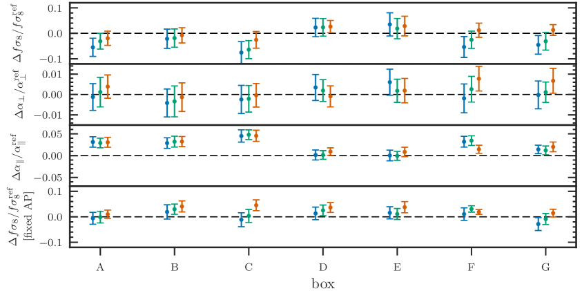
Figure 11: The fractional deviation of the best-fitting $f\sigma_{8}$, $\alpha_{\perp}$, and $\alpha_{\parallel}$ values from their true values for each of the seven lettered challenge boxes. We also show the deviations for $f\sigma_{8}$ obtained when the AP parameters are fixed to their true values. For each box, we show results obtained using (from left to right) $k_{\mathrm{max}}$ = 0.2 (blue), 0.3 (green), and 0.4 (orange)$\ h\text{Mpc}^{-1}$. Error bars show the $1\sigma$ uncertainty as obtained via MCMC sampling.

5.3 Tests on realistic DR12 BOSS CMASS mocks

Finally, we test our RSD model using BOSS DR12 CMASS mock catalogs, using the 84 independent, N-series cutsky catalogs described in §2.2. This set of catalogs offers a chance to test the performance of our model in a realistic setting with a large enough number of catalogs to identify systematic biases up to the level of $\sqrt{84}=9.16$ times smaller than the measurement uncertainty from a single mock. The 84 N-cutsky catalogs accurately model the geometry, volume, and redshift distribution of the DR12 CMASS NGC sample [70]. We use the window function convolution procedure outlined in section 4.3.2 to properly account for effects of the selection function on the measured power spectrum multipoles. We measure the monopole, quadrupole, and hexadecapole for each of the 84 catalogs and estimate the best-fitting model parameters using MAP optimization via the LBFGS algorithm. The power spectra have been measured using FKP weights with a value of $P_{0}=10^{4}$ $[h^{-3}\mathrm{Mpc}^{3}]$. Similar to previous fits, we report parameter constraints as a function of the maximum wavenumber included in the fits. The minimum wavenumber included in the fits is $k_{\mathrm{min}}=0.02\ h\text{Mpc}^{-1}$, chosen to minimize any large-scale effects of the window function on our parameter fits.

We plot the best-fitting $\ell=0$, $2$, $4$, and $6$ theoretical model and the measurements multipoles from a single catalog of the full 84 N-series cutsky test suite in figure 12. Here, the best-fit model has been estimated using the data vector $[P_{0},P_{2},P_{4}]$ with $k_{\mathrm{max}}=0.4\ h\text{Mpc}^{-1}$, but we also show the tetra-hexadecapole ($\ell=6$) to illustrate that the model can accurately predict this higher-order multipole and that it contains little measurable signal. For this single mock, we find good agreement between theory and data, with a reduced chi-squared of $\chi^{2}_{\mathrm{red}}=1.01$.

We give the mean (with the expected value subtracted) and standard deviation of the best-fitting cosmological parameters from fits to each of the 84 cutsky mocks in table 7. We also show the the 1D histograms and 2D correlations of $f\sigma_{8}$, $\alpha_{\perp}$, and $\alpha_{\parallel}$ for the individual fits in figure 13, illustrating the constraining power of our model for these parameters as well as the correlations between the parameters. When fitting the monopole, quadrupole, and hexadecapole, we find good agreement between the mean of the recovered values for $f\sigma_{8}$, $\alpha_{\perp}$, and $\alpha_{\parallel}$. When including scales up to $k_{\mathrm{max}}=0.4\ h\text{Mpc}^{-1}$, we find modest mean biases of $\Delta\langle f\sigma_{8}\rangle=0.005$, $\Delta\langle\alpha_{\perp}\rangle=-0.004$, and $\Delta\langle\alpha_{\parallel}\rangle=0.004$, which represent 14%, 28%, and 17% of the expected mock-to-mock dispersion of each parameter, respectively. The statistical precision of the mean values due to the finite number of catalogs is $84^{-1/2}\simeq 0.1$ times the mock-to-mock dispersion. Thus, the results show evidence for a small bias in the derived $\alpha_{\perp}$ value and marginal evidence for small biases in $\alpha_{\parallel}$ and $f\sigma_{8}$. We also show results in table 7 when fitting only the monopole and quadrupole in order to help quantify the impact of the hexadecapole on our final constraints. The mean best-fitting parameters remain consistent with the results obtained when fitting [$P_{0}$, $P_{2}$, $P_{4}$], and we find the standard deviation of our best-fitting $f\sigma_{8}$ values inflates by roughly 30%, consistent with the findings of [39]. When fixing the AP parameters to their true values, we find that the hexadecapole adds negligible further information to our parameter constraints.

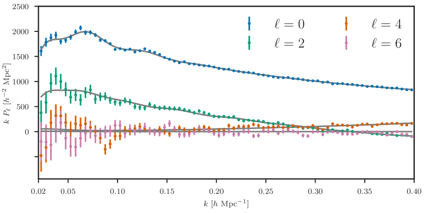
Figure 12: The best-fitting $\ell=0$, $2$, $4$, and $6$ theory (grey lines) and measurements (points with errors) from a single catalog of the N-series cutsky test suite, which accurately simulates the BOSS DR12 CMASS data set. The best-fit model has been estimated using the data vector $[P_{0},P_{2},P_{4}]$ while fitting over the wavenumber range $k=0.02-0.4\ h\text{Mpc}^{-1}$. We also show the tetra-hexadecapole ($\ell=6$) to illustrate that the model can accurately predict this higher-order multipole and that it contains little measurable signal. The reduced chi-squared of the fit for this mock catalog is $\chi^{2}_{\mathrm{red}}=1.01$.

statistics	$k_{\mathrm{max}}$	$\Delta\langle\alpha_{\parallel}\rangle$	$S_{\alpha_{\parallel}}$	$\Delta\langle\alpha_{\perp}\rangle$	$S_{\alpha_{\perp}}$	$\Delta\langle f\sigma_{8}\rangle$	$S_{f\sigma_{8}}$	$\Delta\langle f\sigma_{8}\rangle$	$S_{f\sigma_{8}}$
	[$\ h\text{Mpc}^{-1}$]							fixed AP
[$P_{0}$, $P_{2}$, $P_{4}$]	$0.2$	$0.006\,549\,315\,813\,21$	$0.023\,912\,128\,707\,1$	$-0.004\,120\,642\,391\,64$	$0.015\,735\,340\,980\,6$	$-0.019\,837\,594\,214\,6$	$0.040\,860\,891\,940\,4$	$-0.007\,940\,092\,348\,47$	$0.034\,221\,137\,668\,6$
	$0.3$	$0.007\,401\,943\,495\,92$	$0.025\,427\,825\,779\,7$	$-0.005\,004\,000\,199\,6$	$0.015\,210\,758\,409\,6$	$-0.007\,727\,421\,681\,62$	$0.038\,522\,306\,299\,6$	$0.004\,913\,384\,539\,09$	$0.029\,719\,430\,205\,2$
	$0.4$	$0.004\,082\,238\,129\,01$	$0.023\,147\,263\,871\,8$	$-0.004\,333\,947\,368\,16$	$0.014\,314\,791\,821\,4$	$0.005\,023\,581\,074\,03$	$0.035\,608\,574\,163\,7$	$0.012\,709\,515\,966\,5$	$0.027\,205\,255\,781\,1$
[$P_{0}$, $P_{2}$]	$0.2$	$-0.003\,599\,343\,992\,45$	$0.039\,442\,133\,760\,4$	$-0.000\,968\,386\,304\,057$	$0.018\,642\,581\,673\,4$	$-0.014\,215\,612\,189\,9$	$0.052\,111\,881\,010\,6$	$-0.012\,956\,542\,986\,7$	$0.035\,062\,274\,781\,5$
	$0.3$	$0.004\,857\,719\,726\,06$	$0.040\,838\,660\,942\,9$	$-0.004\,459\,604\,496\,09$	$0.019\,051\,341\,690\,8$	$-0.005\,159\,714\,988\,36$	$0.053\,063\,418\,321\,2$	$0.004\,689\,415\,553\,63$	$0.030\,473\,970\,980\,5$
	$0.4$	$0.011\,887\,291\,251\,2$	$0.036\,261\,299\,937\,8$	$-0.008\,374\,350\,263\,34$	$0.016\,040\,132\,955$	$-0.010\,484\,570\,929\,7$	$0.040\,181\,869\,701\,7$	$0.006\,691\,957\,527\,2$	$0.025\,023\,659\,981$

Table 7: The mean and standard deviation of the best-fitting values for $f\sigma_{8}$, $\alpha_{\perp}$, and $\alpha_{\parallel}$ from fits to the 84 N-series cutsky catalogs. Results are reported as a function of the maximum wavenumber included in the fit. We show results obtained when including or excluding the hexadecapole from our fits in order to quantify the influence of the hexadecapole on our derived constraints.

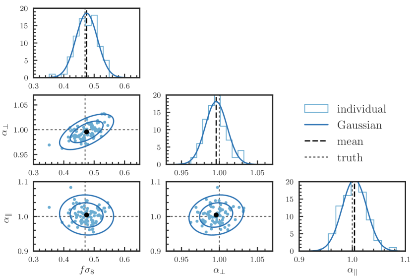
Figure 13: The best-fitting $f\sigma_{8}$, $\alpha_{\perp}$, and $\alpha_{\parallel}$ parameters from fitting our RSD model to the measured $[P_{0},P_{2},P_{4}]$ multipoles from the 84 N-series cutsky mocks. We include wavenumbers in the range $0.02\ h\text{Mpc}^{-1}\leq k\leq 0.4\ h\text{Mpc}^{-1}$. The diagonal panels show the histogram of the recovered parameters, with the mean best-fitting parameters indicated as black dashed lines and the true values as gray dotted lines. The panels below the diagonal show 2D plots with the 84 individual best-fitting parameters as blue dots and the mean as a filled circle. We also show a Gaussian fit to the marginalized parameter distributions in all panels.

5.4 Comparison to published models

	$k_{\mathrm{max}}$ for $[P_{0},P_{2},P_{4}]$	$\Delta\langle\alpha_{\parallel}\rangle$	$S_{\alpha_{\parallel}}$	$\Delta\langle\alpha_{\perp}\rangle$	$S_{\alpha_{\perp}}$	$\Delta\langle f\sigma_{8}\rangle$	$S_{f\sigma_{8}}$
[39]	[0.15, 0.15, 0.1]	$0.004\,932\,690\,476\,19$	$0.033\,803\,848\,044\,2$	$-0.001\,393\,976\,190\,48$	$0.017\,998\,925\,661$	$-0.004\,853\,976\,190\,48$	$0.037\,456\,688\,158\,9$
[40]	[0.2, 0.2, 0.2]	$0.008\,940\,182\,066\,93$	$0.025\,347\,331\,827\,9$	$-0.003\,010\,582\,868\,47$	$0.017\,546\,886\,007\,8$	$0.000\,120\,513\,175\,586$	$0.038\,306\,821\,216\,9$
This work	[0.15, 0.15, 0.1]	$0.000\,257\,492\,539\,603$	$0.040\,261\,078\,438\,2$	$0.001\,114\,014\,696\,59$	$0.018\,337\,320\,438\,5$	$0.004\,299\,994\,122\,2$	$0.044\,689\,398\,091\,5$
	[0.2, 0.2, 0.2]	$0.006\,549\,315\,813\,21$	$0.023\,912\,128\,707\,1$	$-0.004\,120\,642\,391\,64$	$0.015\,735\,340\,980\,6$	$-0.019\,837\,594\,214\,6$	$0.040\,860\,891\,940\,4$
	[0.3, 0.3, 0.3]	$0.007\,401\,943\,495\,92$	$0.025\,427\,825\,779\,7$	$-0.005\,004\,000\,199\,6$	$0.015\,210\,758\,409\,6$	$-0.007\,727\,421\,681\,62$	$0.038\,522\,306\,299\,6$
	[0.4, 0.4, 0.4]	$0.004\,082\,238\,129\,01$	$0.023\,147\,263\,871\,8$	$-0.004\,333\,947\,368\,16$	$0.014\,314\,791\,821\,4$	$0.005\,023\,581\,074\,03$	$0.035\,608\,574\,163\,7$

Table 8: The mean (with expected value subtracted) and standard deviation of the best-fitting cosmology parameters for the 84 N-cutsky mocks using the model in this work as well as the Fourier space models described in [39] and [40]. Results in all cases were computed using FKP weights with $P_{0}=10^{4}\ h^{-3}\mathrm{Mpc}^{3}$.

The set of 84 N-series mocks described in the previous section were utilized as part of the BOSS collaboration’s internal RSD modeling tests in preparation for the DR12 parameter constraint analyses. This enables us to perform a direct comparison of our model with the main Fourier space RSD models used in the DR12 consensus results, which are described in the companion papers in [39] and [40] and the main DR12 consensus paper in [9]. The model used in [40] was also applied to BOSS DR12 data in configuration space, with results presented in [38]. These analyses differ in a number of ways from ours. In particular, these models have significantly fewer parameters (7-8 instead of 13) and use a smaller $k_{\mathrm{max}}$ value in their fits. We limit our fitting range to the same as those used in these works and directly compare the derived parameter constraints for the N-cutsky mocks in table 8. For comparison, this table also includes results from fits using our model that include scales to $k_{\mathrm{max}}=0.3\ h\text{Mpc}^{-1}$ and $k_{\mathrm{max}}=0.4\ h\text{Mpc}^{-1}$, which goes beyond the scales used in [40] and [39]. When using comparable fitting ranges, we find that our model yields a standard deviation for $f\sigma_{8}$ that is larger by $\sim$10% and $\sim$20% as compared to when using the models of [39] and [40], respectively. We find comparable constraints on $f\sigma_{8}$ when extending our model to $k_{\mathrm{max}}=0.3\ h\text{Mpc}^{-1}$ and a modest 5-10% improvement when using $k_{\mathrm{max}}=0.4\ h\text{Mpc}^{-1}$.

For the AP parameters, we find a comparable constraint on $\alpha_{\perp}$ and a slighter worse constraint on $\alpha_{\parallel}$ as compared to the model of [39]. We find modest 5% and 10% reductions in the error on $\alpha_{\parallel}$ and $\alpha_{\perp}$ as compared to the model of [40]. Extending the fits with our model to $k_{\mathrm{max}}=0.4\ h\text{Mpc}^{-1}$ does not provide much gain for the uncertainty of $\alpha_{\parallel}$, but we do find a roughly 20% reduction in the uncertainty of $\alpha_{\perp}$ as compared to the models of [39] and [40]. As seen in the results of [9], the most powerful method for constraining the AP parameters, and thus $D_{A}(z)$ and $H(z)$, remains a BAO-only analysis that takes advantage of the additional statistical precision gained by the process of density field reconstruction. However, some additional constraining power can be gained from full-shape RSD analyses due the AP effect on sub-BAO scales. Here, the extra information provided by extending the modeling to $k_{\mathrm{max}}=0.4\ h\text{Mpc}^{-1}$ will aid the constraints on $D_{A}(z)$ and $H(z)$ and help de-correlate these parameters.

It is also instructive to compare our results for the N-cutsky mocks to the results published in [110], which fits the monopole and quadrupole of the DR12 CMASS sample with $k_{\mathrm{max}}=0.24\ h\text{Mpc}^{-1}$. The comparison yields similar conclusions as previously. In particular, [110] finds errors of $\sigma_{f\sigma_{8}}=0.038$ and $\sigma_{f\sigma_{8}}=0.022$ when varying and fixing the AP parameters, respectively. These errors are both smaller than the uncertainties derived from our model by $\sim$30% when fitting the monopole and quadrupole over similar wavenumber ranges. The constraints for the AP parameters in [110] are similarly smaller than those from our model by a comparable amount.

And, finally, it is worth noting that the $f\sigma_{8}$ constraints using the model in this work are not competitive with the 2.5% constraint on $f\sigma_{8}$ published in [36], which remains the tightest measurement of $f\sigma_{8}$ in the literature to date. With fixed AP parameters, the work used a simulation-based analysis to model the small-scale correlation function of the DR10 CMASS sample well into the nonlinear regime, down to scales of $\sim$$0.8\ h^{-1}\text{Mpc}$. They relied on simulations to accurately model the galaxy-halo connection whereas we use the analytic, halo model decomposition described in section 4.2. Given the tight constraint on $f\sigma_{8}$ found by [36], one might hope that Fourier space models could be similarly extended into the nonlinear regime and yield comparable increases in precision. However, while acknowledging the number of differences in the two analyses, we note that we do not find such large increases in precision in our measurement of $f\sigma_{8}$ when including small-scale information down to $k=0.4\ h\text{Mpc}^{-1}$.

6 Discussion

The results presented in section 5 provide tests of the RSD model presented in this work for a suite of simulations that span a wide range in both cosmology and galaxy bias models. Given the measurement uncertainties and the degrees of freedom in our model, we are able to achieve excellent agreement between the $\ell=0,2,4$ multipoles measured from simulations and our best-fitting theory down to scales of $k=0.4\ h\text{Mpc}^{-1}$. To quantify the impact of small-scale physics on our model, we perform fits for $k_{\mathrm{max}}=0.2$, $0.3$, and $0.4\ h\text{Mpc}^{-1}$. The results across the different sets of simulations indicate a positive systematic shift in the parallel AP parameter $\alpha_{\parallel}$ at the level of $0.01-0.02$ that is independent of the $k_{\mathrm{max}}$ value used. For fits using $k_{\mathrm{max}}=0.4\ h\text{Mpc}^{-1}$, we find small biases at the level of $\sim$0.005 for $f\sigma_{8}$ and $\alpha_{\perp}$. These deviations are small and can be effectively calibrated with simulations. The amplitude of the shifts is similar to the level of theoretical systematics present when using other RSD models in the literature, i.e., [9]. The positive bias in $\alpha_{\parallel}$ propagates into a small bias in $f\sigma_{8}$ when fixing the AP parameters to their expected values, due to the anti-correlation between $f\sigma_{8}$ and $\alpha_{\parallel}$. The exact amplitude of the bias in $\alpha_{\parallel}$ can be robustly estimated from a larger set of simulations than is considered in this work and the best-fitting $\alpha_{\parallel}$ value modified accordingly, while accounting for the systematic uncertainty in the error budget.

A primary goal of this work is to ensure that any model parameters that we introduce have physically meaningful values and are not just nuisance parameters. We attempt to capture the complex effects of satellite galaxies on the clustering signal in redshift space by considering separately the clustering of isolated satellites and those that live in halos with at least two satellites. This parametrization leads to a total of 13 model parameters, significantly more than other Fourier space RSD models in the literature, i.e., [39, 40], which typically only have 7-8 parameters. In addition to differences in the treatment of RSD and perturbation theory choices, perhaps the most significant difference is the use of a single parameter to model the nonlinear FoG effect of the full galaxy sample, instead of separately modeling the effects for central and satellite subsamples, as is done in this work. They also typically float a constant, shot noise parameter, designed to absorb any potential deficiencies in the model. In some sense, these models are a limit of the more general parametrization considered in this work and are only valid over a certain range of scales and galaxy bias values.

As demonstrated in the analysis of [9], the level of theoretical errors in $f\sigma_{8}$ measurements from full-shape RSD analyses ranges from $\sim$25-50% of the statistical precision for the three redshift bins considered for the completed BOSS DR12 sample. Another recent analysis [111] provides evidence for the possible shortcomings of the RSD model of [39]. The work extends the modeling to include the relative velocity effect of baryons and cold dark matter at decoupling but fails several null tests. The systematics situation is perhaps even more dire when considering the fact that background cosmology model is essentially fixed by the Planck results (see Fig. 11 of [9]), indicating that a more relevant test of systematics should be done with the AP parameters fixed, often resulting in a $\sim$20-30% smaller error on $f\sigma_{8}$. This suggests that RSD analyses from full-shape modeling are already systematics dominated and will certainly be so for future galaxy surveys, without subsequent modeling improvements. While the model presented in this work has its own shortcomings, one such avenue for improvement is exploring more physically motivated model descriptions.

As discussed in section 5.4, our parametrization leads to a derived uncertainty of $f\sigma_{8}$ that is roughly 10-20% larger than the constraint from the models of [39, 40], which use fewer parameters. Each of our parameters has a physical motivation, and we apply reasonable priors based on these motivations when appropriate. Thus, we find no clear path to reduce the number of parameters in our model and do not believe that additional constraining power can be gained through the use of stronger priors. As such, RSD models in the literature are likely too-limited in their parametrization, with the uncertainty on $f\sigma_{8}$ underestimated by $\sim$10-20%. For a galaxy sample such as the BOSS CMASS sample with a satellite fraction $f_{s}\sim 0.1$, the clustering is dominated by the 2-halo correlations of centrals. However, we find the inclusion of parameters to properly treat the 1% effects of satellite-satellite correlations to be crucial to modeling the clustering down to scales of $k\sim 0.4\ h\text{Mpc}^{-1}$. Using a Fisher analysis, we find similar errors on $f\sigma_{8}$ as found by the models of [39, 40] for the N-cutsky mocks (see table 8) when fixing the relative fraction of non-isolated satellites $f_{s_{B}}$ and the central galaxy velocity dispersion $\sigma_{c}$. In this case, we only vary a single FoG velocity dispersion, as is the case for the models of [39, 40], and fix the $\sim$1% contribution to the overall power spectrum from satellites living in halos containing multiple satellites.

Fully perturbative modeling approaches cannot accurately capture the effects of nonlinearities, i.e., the FoG effect from satellites, on small scales, and at some point, the modeling must become sensitive to the poorly-understood physics of galaxy evolution. Presently, it is unclear how sensitive cosmological growth of structure measurements are to such small-scale physics. In particular, assembly bias remains a worrying potential systematic for galaxy clustering analyses [112, 113]. The most promising avenue for including small-scale information ($k\sim 0.4\ h\text{Mpc}^{-1}$) in growth of structure analyses appears to be simulation-based modeling efforts. The most competitive constraint to date for $f\sigma_{8}$ published in [36] uses a simulation-based model to describe the correlation function down to scales of $r\sim 0.8\ h^{-1}\text{Mpc}$. In order to achieve the desired accuracy for the RSD model presented in this work, we also find it necessary to include calibrations from simulations for key components of the model. The combination of perturbation theory with simulation-based calibration in our model likely limits the applicability of the model in comparison to a fully general, simulation-based approach. An emulator-based approach for the nonlinear clustering of galaxies in redshift-space using the FastPM simulation method [114] is under active development.

An alternative approach for maximizing the constraining power of RSD analyses relies on limiting the effects of satellites on the modeling. These so-called halo reconstruction methods attempt to modify the measurement procedure to preferentially exclude satellites galaxies, thus measuring the clustering of the underlying halo density field, rather than the galaxy density field [27, 115, 116]. The difficulty of these methods remains achieving a transformation accurate enough such that the added modeling complications from the transformation itself do not outweigh the benefits gained by removing satellites. The advantages include limiting the effects of nonlinearities, which simplifies the modeling and could allow use of models closer to purely linear theory. Reducing FoG effects raises the overall amplitude of the quadrupole and boosts the signal-to-noise of the measurement, although removing satellite galaxies does lower the overall bias, which reduces the constraining power of a given measurement.

As an illustration, we have compared our RSD constraints when fitting our 13 parameter model to the clustering of centrals and type A centrals (isolated centrals that have no satellites) from the RunPB simulations. We show the best-fit multipoles for these cases in comparison to the spectra of the full galaxy sample in figure 14. As expected, the small-scale quadrupole shows a significant reduction in the effects of RSD, and we find a reduction in the linear bias due to the removal of the highly biased satellites. Corresponding parameter constraints for $f\sigma_{8}$, $\alpha_{\perp}$, and $\alpha_{\parallel}$ are presented in table 9. We find the largest decreases in uncertainty when considering centrals only – the error on $f\sigma_{8}$ decreases by 31%, 19%, and 15% when fitting to $k_{\mathrm{max}}=0.2,0.3$, and $0.4\ h\text{Mpc}^{-1}$, respectively. Similarly, we find decreases of 16%, 7%, and 25% for $\alpha_{\parallel}$ and 19%, 10%, and 0% for $\alpha_{\perp}$. While we find diminishing benefits to extending the fitting range from $k_{\mathrm{max}}=0.2\ h\text{Mpc}^{-1}$ to $k_{\mathrm{max}}=0.4\ h\text{Mpc}^{-1}$, the constraints using centrals only are in all cases better than using when using all galaxies. Furthermore, fitting the clustering of only centrals to $k_{\mathrm{max}}=0.2\ h\text{Mpc}^{-1}$ is roughly as competitive in constraining $f\sigma_{8}$ as fitting the clustering of all galaxies to $k_{\mathrm{max}}=0.4\ h\text{Mpc}^{-1}$, and the latter is significantly more challenging to model than the former. While we recognize that this is certainly an idealized demonstration, we view halo reconstruction methods as an important area of future research for both their constraining power and simplified theoretical modeling.

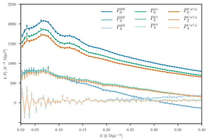
Figure 14: The best-fitting model and measured simulation points for the monopole (darkest shade), quadrupole, and hexadecapole (lightest shade) from the mean of 10 RunPB galaxy catalogs at $z=0.55$ for all galaxies $P_{\ell}^{gg}$ (blue), all centrals $P_{\ell}^{cc}$ (green), and isolated centrals with no satellites in the same halo $P_{\ell}^{c_{A}c_{A}}$ (orange). Linear biases for each sample are $b_{1,g}=2.05$, $b_{1,c}=1.93$, and $b_{1,c_{A}}=1.84$.

$k_{\mathrm{max}}$		all galaxies	centrals only	type A centrals only
$k_{\mathrm{max}}=0.2\ h\text{Mpc}^{-1}$	$\Delta\alpha_{\parallel}$	+$0.008\,968\,110\,671\,99$ ${}^{$0.009\,548\,766\,288\,35$}_{$-0.008\,575\,451\,096\,98$}$	+$0.009\,601\,090\,887\,52$ ${}^{$0.007\,624\,979\,487\,13$}_{$-0.007\,610\,804\,143\,69$}$	+$0.010\,143\,188\,049\,9$ ${}^{$0.008\,149\,444\,135\,81$}_{$-0.008\,070\,022\,640\,33$}$
	$\Delta\alpha_{\perp}$	+$0.002\,880\,197\,951\,87$ ${}^{$0.005\,369\,816\,420\,58$}_{$-0.006\,284\,305\,543\,54$}$	+$0.002\,251\,073\,978\,2$ ${}^{$0.004\,825\,778\,595\,31$}_{$-0.004\,615\,479\,067\,96$}$	+$0.002\,270\,353\,114\,03$ ${}^{$0.004\,665\,503\,198\,12$}_{$-0.004\,653\,516\,529\,35$}$
	$\Delta f\sigma_{8}$	$-0.017\,364\,677\,906$ ${}^{$0.014\,874\,607\,324\,6$}_{$-0.015\,375\,888\,596\,2$}$	$-0.004\,230\,824\,232\,1$ ${}^{$0.010\,804\,653\,167\,7$}_{$-0.010\,043\,650\,865\,6$}$	$-0.008\,948\,949\,098\,59$ ${}^{$0.011\,579\,900\,98$}_{$-0.010\,755\,300\,521\,9$}$
$k_{\mathrm{max}}=0.3\ h\text{Mpc}^{-1}$	$\Delta\alpha_{\parallel}$	+$0.006\,491\,541\,322\,76$ ${}^{$0.007\,784\,376\,829\,3$}_{$-0.007\,363\,477\,268\,73$}$	+$0.004\,918\,744\,535\,64$ ${}^{$0.007\,174\,638\,747\,94$}_{$-0.006\,986\,910\,901\,36$}$	+$0.003\,782\,234\,541\,53$ ${}^{$0.006\,892\,360\,003\,92$}_{$-0.006\,747\,006\,024\,38$}$
	$\Delta\alpha_{\perp}$	+$0.004\,210\,013\,177\,7$ ${}^{$0.004\,924\,848\,083\,96$}_{$-0.004\,572\,192\,752\,07$}$	+$0.004\,382\,168\,979\,89$ ${}^{$0.004\,267\,149\,656\,14$}_{$-0.004\,272\,989\,070\,51$}$	+$0.004\,647\,547\,390\,7$ ${}^{$0.004\,451\,514\,537\,02$}_{$-0.004\,632\,042\,373\,57$}$
	$\Delta f\sigma_{8}$	$-0.004\,797\,619\,700\,43$ ${}^{$0.012\,208\,059\,430\,1$}_{$-0.012\,776\,181\,101\,8$}$	+$0.006\,589\,490\,056\,04$ ${}^{$0.009\,957\,119\,822\,5$}_{$-0.010\,390\,543\,060\,6$}$	+$0.003\,067\,555\,904\,39$ ${}^{$0.009\,298\,413\,991\,93$}_{$-0.009\,346\,038\,103\,1$}$
$k_{\mathrm{max}}=0.4\ h\text{Mpc}^{-1}$	$\Delta\alpha_{\parallel}$	+$0.008\,891\,525\,410\,23$ ${}^{$0.006\,819\,668\,222\,76$}_{$-0.007\,680\,713\,207\,87$}$	+$0.002\,982\,757\,831\,35$ ${}^{$0.005\,524\,014\,071\,04$}_{$-0.005\,408\,351\,529\,38$}$	+$0.001\,193\,582\,780\,34$ ${}^{$0.006\,090\,931\,105\,44$}_{$-0.006\,775\,876\,243\,18$}$
	$\Delta\alpha_{\perp}$	+$0.004\,951\,017\,011\,09$ ${}^{$0.004\,241\,418\,553\,13$}_{$-0.004\,049\,028\,722\,63$}$	+$0.002\,859\,703\,766\,19$ ${}^{$0.004\,442\,837\,926\,95$}_{$-0.003\,883\,528\,719\,33$}$	+$0.001\,198\,880\,299\,37$ ${}^{$0.004\,425\,875\,893\,45$}_{$-0.004\,097\,716\,638\,47$}$
	$\Delta f\sigma_{8}$	$-0.003\,085\,819\,005\,97$ ${}^{$0.009\,673\,357\,009\,89$}_{$-0.009\,075\,522\,422\,79$}$	+$0.003\,093\,364\,715\,58$ ${}^{$0.008\,498\,935\,405\,03$}_{$-0.007\,560\,342\,550\,28$}$	+$0.005\,897\,688\,746\,45$ ${}^{$0.008\,349\,731\,564\,52$}_{$-0.008\,071\,944\,117\,55$}$

Table 9: The best-fit $f\sigma_{8}$, $\alpha_{\perp}$, and $\alpha_{\parallel}$ values and $1\sigma$ uncertainties obtained when fitting the monopole, quadrupole, and hexadecapole from the mean of 10 RunPB galaxy catalogs at $z=0.55$ when including all galaxies, centrals only, and type A centrals only, which are isolated with no satellites in the same halo.

7 Conclusion

We present a new model for the redshift-space power spectrum of galaxies and demonstrate its accuracy in modeling the monopole, quadrupole, and hexadecapole of the galaxy density field down to $k=0.4\ h\text{Mpc}^{-1}$ through a series of tests on high-fidelity $N$-body simulations. The model describes the clustering of galaxies in the context of a halo model, building upon the formalism presented in [58]. We decompose galaxies into four subsamples: centrals with and without satellites and satellites with one or more neighboring satellite. We then model the clustering of the underlying halos in redshift space using a combination of Eulerian perturbation theory and $N$-body simulations. The modeling of RSD via the mapping from real space to redshift space is done using the so-called distribution function approach. In order to achieve sufficient accuracy in the modeling down to $k=0.4\ h\text{Mpc}^{-1}$, we utilize a set of simulations to calibrate the most important terms of the model. To this end, we extend the Halo-Zel’dovich Perturbation Theory of [59], which combines Lagrangian perturbation theory with physically motivated corrections calibrated from simulations. We improve the accuracy of this model for the dark matter density power spectrum and develop models for the dark matter velocity correlators $P_{01}$ and $P_{11}$. Our final model has 13 free parameters, each of which is physically motivated, as described in table 3. The model accounts for the FoG effect from each of our galaxy subsamples, rather than using a single velocity dispersion to describe the combined effect. We account for the linear bias of each of the subsamples and describe the shot noise contributions to the power spectrum via the amplitude of the 1-halo galaxy correlations.

We fit our 13 parameter model to the monopole, quadrupole, and hexadecapole measured from several sets of simulations to test the accuracy and precision of the recovered parameters. These mock catalogs cover a range of cosmologies and galaxy bias models, providing stringent tests of our model. The test suite also includes realistic mock catalogs of the BOSS DR12 CMASS sample, properly modeling the volume and selection effects of this data set. We perform fits as a function of the maximum wavenumber included in the fit, using $k_{\mathrm{max}}=0.2,0.3$, and $0.4\ h\text{Mpc}^{-1}$. The results of these tests can be summarized as follows:

1. Given the measurement covariance and degrees of freedom in the model, we find excellent agreement between our model and the measured $\ell=0$, 2, and 4 multipoles from simulations down to scales of $k=0.4\ h\text{Mpc}^{-1}$.

2. A systematic shift in the best-fitting value of $\alpha_{\parallel}$ is identified at the level of $0.01-0.02$, independent of the $k_{\mathrm{max}}$ value used when fitting. Such a systematic shift can be calibrated from a large set of simulations and a correction applied to the best-fitting value.

3. The level of systematic bias in the parameters $f\sigma_{8}$ and $\alpha_{\perp}$ is found to be small, at the level of $\sim$0.005, which is similar to other published RSD models in the literature, i.e., [9]. However, considering that the Planck results essentially fix the background cosmology model, comparisons between this level of systematics and the error on $f\sigma_{8}$ for fixed AP parameters indicate that RSD analyses are nearly systematics dominated today. This will certainly be the case for the next generation of galaxy surveys, unless analyses are limited to the largest scales or substantial modeling improvements are made.

4. Using a set of BOSS DR12 CMASS mock catalogs as a benchmark for comparison, we estimate an uncertainty on $f\sigma_{8}$ that is $\sim$10-20% larger than when using the models of [39, 40], when fitting over similar wavenumber ranges. With 5-6 fewer parameters, these models likely have a too-limited parametrization and are underestimating the resulting uncertainty of $f\sigma_{8}$.

5. Extending the fitting range to $k_{\mathrm{max}}=0.4\ h\text{Mpc}^{-1}$ provides 15-30% gains in the statistical precision of the $f\sigma_{8}$ constraint relative to $k_{\mathrm{max}}=0.2\ h\text{Mpc}^{-1}$. The gains are more modest when our model is compared to published models, which use a more limited parametrization; the error on $f\sigma_{8}$ is roughly 5-10% smaller with our model using $k_{\mathrm{max}}=0.4\ h\text{Mpc}^{-1}$ than constraints found when using the models of [39, 40] (with $k_{\mathrm{max}}\simeq 0.2\ h\text{Mpc}^{-1}$) for the BOSS DR12 CMASS sample.

6. We find a $\sim$10-15% improvement in the constraint on $\alpha_{\perp}$ and only marginal gains for $\alpha_{\parallel}$ when extending from $k_{\mathrm{max}}=0.2\ h\text{Mpc}^{-1}$ to $k_{\mathrm{max}}=0.4\ h\text{Mpc}^{-1}$. The constraint on $\alpha_{\perp}$ represents a 20% improvement relative to the results found when the published models of [39, 40]. This improvement will further help constrain and de-correlate the parameters $D_{A}(z)$ and $H(z)$ when combined with post-reconstruction BAO-only analyses.

Extending full-shape RSD modeling of galaxy clustering to smaller scales in both an accurate and precise manner remains a complicated endeavor. Applying models such as the one presented here will be necessary at the minimum to fully capitalize on the cosmological information contained in future galaxy surveys, such as Hobby Eberly Telescope Dark Energy Experiment [117], the Dark Energy Spectroscopic Instrument (DESI)[118], the Subaru Prime Focus Spectrograph [119], and the ESA space mission Euclid [120]. For example, we expect our model to perform well on the DESI Emisson Line Galaxy sample, which has a lower bias and high satellite fraction as compared to the BOSS CMASS sample. Conversely, the gains when applying our model to next generation quasar samples would likely be more modest due to the high shot noise and lower impact of one-halo correlations.

There are several intriguing modeling approaches that can go beyond our analytic modeling approach and potentially improve the constraints further. Simulation-based approaches can leverage advances in high-performance computing to accurately model nonlinear clustering on small-scales. Complementary approaches such as halo reconstruction can simplify modeling and reduce the need to include small-scale information by mitigating the complicated effects of satellite galaxies on the modeling procedure. It remains to be seen if these further advances will improve cosmological constraints, or whether with our model we have reached the limit due to the effects of nonlinear evolution and poorly known small-scale physics.

Appendix A Velocity correlators in the Zel’dovich approximation

In this section, we use Lagrangian perturbation theory (LPT) to compute two dark matter velocity correlators that enter into the DF model: the density – radial momentum cross spectrum, $P_{01}$, and the radial momentum auto spectrum, $P_{11}$. We closely follow the notation of [94]; see e.g, [94, 121, 122] and references therein for further review of Lagrangian perturbation theory.

A.1 $P_{01}$ and $P_{11}$ using LPT

Following the definitions of [54], the velocity correlators that we wish to compute are given by

$$(2\pi)^{3}P_{01}(k)\delta^{D}(\mathbf{k}+\mathbf{k}^{\prime}) = \langle\delta(\mathbf{k})|p_{\parallel}(\mathbf{k}^{\prime})\rangle,$$

$$(2\pi)^{3}P_{11}(k)\delta^{D}(\mathbf{k}+\mathbf{k}^{\prime}) = \langle p_{\parallel}(\mathbf{k})|p_{\parallel}(\mathbf{k}^{\prime})\rangle,$$ (A.1)

where $p_{\parallel}$ is the momentum projected along the line-of-sight, i.e., $p_{\parallel}=\mathbf{p}\cdot\hat{z}$. The scalar component of the dark matter momentum (which correlates with density) can be computed using the continuity equation: $\dot{\delta}(\mathbf{k})-i\mathbf{k}\cdot\mathbf{p}=0$, where the dot in $\dot{\delta}$ represents the derivative with respect to conformal time $\tau$. Using this equation, we can express the velocity correlators of interest as

$$P_{01}(k) = \frac{i\mu}{k}P_{\delta\dot{\delta}}(k),$$ (A.2)

$$P_{11,s}(k) = \frac{\mu^{2}}{k^{2}}P_{\dot{\delta}\dot{\delta}}(k),$$ (A.3)

where $\mu$ is defined as $k_{\parallel}/k$. Here, we explicitly note that $P_{11,s}$ only includes scalar contributions, as only the scalar component of momentum enters into the continuity equation. The total contribution from these terms to the redshift-space power spectrum $P^{S}(k,\mu)$ is given by:

$$P_{01}^{S}(\mathbf{k}) = 2\mathrm{Re}\left(\frac{-ik\mu}{\mathcal{H}}\right)P_{01}(k)=2\frac{\mu^{2}}{\mathcal{H}}P_{\delta\dot{\delta}}(k),$$ (A.4)

$$P_{11,s}^{S}(\mathbf{k}) = \left(\frac{k\mu}{\mathcal{H}}\right)^{2}P_{11,s}(k)=\frac{\mu^{4}}{\mathcal{H}^{2}}P_{\dot{\delta}\dot{\delta}}(k).$$ (A.5)

These are the spectra that we wish to compute in the Zel’dovich approximation. In linear theory, these spectra are the anisotropic terms of the well-known Kaiser formula: $P_{01}^{S}(\mathbf{k})=2f\mu^{2}P_{L}(k)$ and $P_{11,s}^{S}(\mathbf{k})=f^{2}\mu^{4}P_{L}(k)$ [19].

We can compute $\delta$ and $\dot{\delta}$ using Lagrangian perturbation theory. In the Lagrangian clustering description, the overdensity field is given by

$$(2\pi)^{3}\delta^{D}(\mathbf{k})+\delta(\mathbf{k})=\int d^{3}q\ e^{i\mathbf{k}\cdot\mathbf{q}}\exp[i\mathbf{k}\cdot\Psi(\mathbf{q})],$$ (A.6)

where $\Psi(\mathbf{q})$ is the Lagrangian displacement field. The derivative of this equation with respect to conformal time is given by

$$\dot{\delta}(\mathbf{k})=\int d^{3}qe^{i\mathbf{k}\cdot\mathbf{q}}\left(i\mathbf{k}\cdot\dot{\Psi}\right)\exp[i\mathbf{k}\cdot\Psi(\mathbf{q})].$$ (A.7)

The quantity of interest for $P_{01}$ is

$$(2\pi)^{3}P_{\delta\dot{\delta}}(k)\delta^{D}(\mathbf{k}+\mathbf{k}^{\prime}) = \langle\delta(\mathbf{k})|\dot{\delta}(\mathbf{k}^{\prime})\rangle,$$ (A.8)

$$= \int d^{3}qd^{3}q^{\prime}e^{i\mathbf{k}\cdot\mathbf{q}+i\mathbf{k}^{\prime}\cdot\mathbf{q}^{\prime}}\left\langle\left(i\mathbf{k}^{\prime}\cdot\dot{\Psi}^{\prime}\right)e^{i\mathbf{k}\cdot\Psi+i\mathbf{k}^{\prime}\cdot\Psi^{\prime}}\right\rangle,$$

where we have used the definition $\Psi^{\prime}\equiv\Psi(\mathbf{q}^{\prime})$. Similarly, for $P_{11,s}$ we need to compute

$$(2\pi)^{3}P_{\dot{\delta}\dot{\delta}}(k)\delta^{D}(\mathbf{k}+\mathbf{k}^{\prime}) = \langle\dot{\delta}(\mathbf{k})|\dot{\delta}(\mathbf{k}^{\prime})\rangle,$$ (A.9)

$$= \int d^{3}qd^{3}q^{\prime}e^{i\mathbf{k}\cdot\mathbf{q}+i\mathbf{k}^{\prime}\cdot\mathbf{q}^{\prime}}\left\langle\left(i\mathbf{k}\cdot\dot{\Psi}\right)\left(i\mathbf{k}^{\prime}\cdot\dot{\Psi}^{\prime}\right)e^{i\mathbf{k}\cdot\Psi+i\mathbf{k}^{\prime}\cdot\Psi^{\prime}}\right\rangle.$$

A.2 A generalized velocity generating function

To facilitate the calculation of equations A.6 and A.7, we introduce a generalized velocity generating function in this section. First, let us define the sum and difference of the displacement field $\Psi(\mathbf{q})$ defined at points $\mathbf{q}_{1}$ and $\mathbf{q}_{2}$ in space:

$$\Delta_{i}^{-}=\Psi_{i}(\mathbf{q}_{2})-\Psi_{i}(\mathbf{q}_{1}),\ \ \ \ \Delta_{i}^{+}=\Psi_{i}(\mathbf{q}_{2})+\Psi_{i}(\mathbf{q}_{1}).$$ (A.10)

Now we can define the generalized velocity generating function $\mathcal{G}$ as

$$(2\pi)^{3}\delta^{D}(\mathbf{k})=\mathcal{G}(k,\gamma,\lambda)=\int d^{3}qe^{i\mathbf{k}\cdot\mathbf{q}}\left\langle e^{-i\mathbf{k}\cdot\Delta^{-}-i\gamma\mathbf{k}\cdot\dot{\Delta}^{-}-i\lambda\mathbf{k}\cdot\dot{\Delta}^{+}}\right\rangle.$$ (A.11)

Note that the case of $\gamma=\lambda=0$ gives the well-known matter power spectrum $P_{\delta\delta}$ in the LPT formalism [123]. We define the following moments of $\mathcal{G}$:

$$G_{10}(k) = \frac{d}{d\gamma}\mathcal{G}(k,\gamma,\lambda)\Big{|}_{\gamma=0,\lambda=0}=\int d^{3}qe^{i\mathbf{k}\cdot\mathbf{q}}\left\langle\left(i\mathbf{k}\cdot\dot{\Delta}^{-}\right)e^{-i\mathbf{k}\cdot\dot{\Delta}^{-}}\right\rangle,$$ (A.12)

$$G_{20}(k) = \frac{d^{2}}{d\gamma^{2}}\mathcal{G}(k,\gamma,\lambda)\Big{|}_{\gamma=0,\lambda=0}=\int d^{3}qe^{i\mathbf{k}\cdot\mathbf{q}}\left\langle\left(i\mathbf{k}\cdot\dot{\Delta}^{-}\right)^{2}e^{-i\mathbf{k}\cdot\dot{\Delta}^{-}},\right\rangle,$$ (A.13)

$$G_{02}(k) = \frac{d^{2}}{d\lambda^{2}}\mathcal{G}(k,\gamma,\lambda)\Big{|}_{\gamma=0,\lambda=0}=\int d^{3}qe^{i\mathbf{k}\cdot\mathbf{q}}\left\langle\left(i\mathbf{k}\cdot\dot{\Delta}^{+}\right)^{2}e^{-i\mathbf{k}\cdot\dot{\Delta}^{-}},\right\rangle.$$ (A.14)

Substituting the definitions of $\Delta^{+}$ and $\Delta^{-}$ into these equations yields the following relations,

$$G_{10}(k)=2P_{\delta\dot{\delta}}(k),$$ (A.15)

$$G_{20}(k)+G_{02}(k)=4P_{\dot{\delta}\dot{\delta}}(k).$$ (A.16)

We can evaluate $\mathcal{G}$ using the cumulant expansion theorem,

$$\left\langle e^{iX}\right\rangle=\exp\left[\sum_{N=0}^{\infty}\frac{(-i)^{N}}{N!}\left\langle X^{N}\right\rangle\right],$$ (A.17)

where $X=\mathbf{k}\cdot\Delta^{-}+\gamma\mathbf{k}\cdot\dot{\Delta}^{-}+\lambda\mathbf{k}\cdot\dot{\Delta}^{+}$. In the Zel’dovich approximation (tree-level LPT), the displacement field remains Gaussian, so only the $N=2$ term is non-zero in the above expansion. Thus, the quantity of interest is

$$\left\langle\left(\mathbf{k}\cdot\Delta^{-}+\gamma\mathbf{k}\cdot\dot{\Delta}^{-}+\lambda\mathbf{k}\cdot\dot{\Delta}^{+}\right)^{2}\right\rangle = k_{i}k_{j}\left[A_{ij}+\gamma\dot{A}_{ij}+\gamma^{2}B_{ij}^{-}+\lambda^{2}B_{ij}^{+}+...\right]$$ (A.18)

$$= k_{i}k_{j}\left[\mathcal{A}_{ij}+...\right],$$

where we have explicitly ignored terms that vanish upon taking the derivatives in the expressions for $G_{10}$, $G_{20}$, and $G_{02}$. The relevant definitions are

$$A_{ij}(k) = \left\langle\Delta^{-}_{i}\Delta^{-}_{j}\right\rangle_{c},$$ (A.19)

$$B_{ij}^{-}(k) = \left\langle\dot{\Delta}^{-}_{i}\dot{\Delta}^{-}_{j}\right\rangle_{c},$$ (A.20)

$$B_{ij}^{+}(k) = \left\langle\dot{\Delta}^{+}_{i}\dot{\Delta}^{+}_{j}\right\rangle_{c}.$$ (A.21)

Note that this definition of $A_{ij}$ matches the notation used in the recent LPT work of [94, 121]. Finally, using equations A.18, A.17, and A.11, the velocity generating function becomes

$$(2\pi)^{3}\delta^{D}(\mathbf{k})+\mathcal{G}(k,\gamma,\lambda)=\int d^{3}qe^{i\mathbf{k}\cdot\mathbf{q}}\exp\left[-\frac{1}{2}k_{i}k_{j}\mathcal{A}_{ij}\right].$$ (A.22)

A.3 The Zel’dovich approximation

In the Zel’dovich approximation, the displacement field and its time derivative are given

$$\Psi(\mathbf{k}) = -i\mathbf{k}\delta_{L}(\mathbf{k})/k^{2},$$ (A.23)

$$\dot{\Psi}(\mathbf{k}) = f\mathcal{H}\Psi(\mathbf{k}),$$ (A.24)

where $\delta_{L}$ is the linear overdensity field which scales in time as the linear growth function $D$, $\mathcal{H}=d\ln a/d\tau$ is the conformal Hubble parameter, and $f=d\ln D/d\ln a$ is the logarithmic growth rate.

With these relations, we can now compute the expressions for term of A.18 (for a more in-depth discussion of this procedure, see Appendix B of [121]). The relevant expressions are:

$$A_{ij}(\mathbf{q}) = I_{ij}^{-}(\mathbf{q}),$$ (A.25)

$$\dot{A}_{ij}(\mathbf{q}) = 2f\mathcal{H}I_{ij}^{-}(\mathbf{q}),$$ (A.26)

$$\dot{B}_{ij}^{-}(\mathbf{q}) = (f\mathcal{H})^{2}I_{ij}^{-}(\mathbf{q}),$$ (A.27)

$$\dot{B}_{ij}^{+}(\mathbf{q}) = (f\mathcal{H})^{2}I_{ij}^{+}(\mathbf{q}),$$ (A.28)

where we have defined the integral

$$I_{ij}^{\pm}(\mathbf{q})=2\int\frac{d^{3}k}{(2\pi)^{3}}\left[1\pm\cos(\mathbf{k}\cdot\mathbf{q})\right]\frac{k_{i}k_{j}}{k^{4}}P_{L}(k),$$ (A.29)

where $P_{L}(q)$ is the linear power spectrum. Here, $I_{ij}^{-}$ is the same quantity that enters into the LPT calculation of the density auto power spectrum; for example, our expression is the same as equation A6 of [94] (restricting to tree-level).

Equation A.29 can be expressed in terms of two scalar functions as

$$X_{ij}^{\pm}(\mathbf{q})=X^{\pm}(q)\delta^{K}_{ij}+Y^{\pm}(q)\hat{q}_{i}\hat{q}_{j},$$ (A.30)

We can compute $X_{ij}^{\pm}$ and $Y_{ij}^{\pm}$ by performing the angular integration in equation A.29. To facilitate comparisons with previous work (e.g., [94, 121]), we define

$$X_{ij}^{\pm}(q) = 2\sigma^{2}\pm\frac{1}{\pi^{2}}\int dkP_{L}(k)\frac{j_{1}(kq)}{kq}\equiv 2\sigma^{2}\pm X_{0}(q),$$

$$X_{ij}^{-}(q) = X(q),$$

$$Y_{ij}^{\pm}(q) = \mp Y(q),$$ (A.31)

where the $\sigma^{2}=1/(6\pi^{2})\int dqP(q)$ is the square of the linear displacement field dispersion, and the well-known Zel’dovich integrals $X(q)$ and $Y(q)$ are

$$X(q) = \int\frac{dk}{2\pi^{2}}P_{L}(k)\left[\frac{2}{3}-2\frac{j_{1}(kq)}{kq}\right],$$

$$Y(q) = \int\frac{dk}{2\pi^{2}}P_{L}(k)\left[-2j_{0}(kq)+6\frac{j_{1}(kq)}{kq}\right],$$ (A.32)

where $j_{n}$ is the spherical Bessel function of order $n$.

With these integral expressions, we can now compute the relevant moments of $\mathcal{G}$ in order to evaluate $P_{01}^{S}$ and $P_{11,s}^{S}$. First, for $P_{01}^{S}$, we have

$$P_{01}^{S}(k,\mu) =\frac{\mu^{2}}{\mathcal{H}}G_{10}(k),$$

$$=2f\mu^{2}\int d^{3}qe^{ikq\bar{\mu}}\left[-\frac{1}{2}k^{2}\left(X+\bar{\mu}^{2}Y\right)\right]e^{-\frac{1}{2}k^{2}(X+\bar{\mu}^{2}Y)},$$ (A.33)

where we have introduced the angle between the given $k$-mode and separation vector $\bar{\mu}=\hat{q}\cdot\hat{k}$. Similarly, for $P_{11,s}^{S}$, we have

$$P_{11,s}^{S}(k,\mu) =\frac{\mu^{4}}{4\mathcal{H}^{2}}\left[G_{20}(k)-G_{02}(k)\right],$$

$$=\frac{1}{4}f^{2}\mu^{4}\int d^{3}qe^{ikq\bar{\mu}}k^{2}\left[-2X_{0}+k^{2}X^{2}+2(k^{2}X-1)Y\bar{\mu}^{2}+k^{2}Y^{2}\bar{\mu}^{4}\right]e^{-\frac{1}{2}k^{2}(X+\bar{\mu}^{2}Y)}.$$ (A.34)

Equations A.33 and A.34 represent the desired solution for $P_{01}^{S}$ and $P_{11,s}^{S}$ in the Zel’dovich approximation. The angular integration over $\bar{\mu}$ in these expressions can be performed using the following expression [123]

$$\int_{-1}^{1}d\mu e^{iA\mu}e^{B\mu^{2}}=2e^{B}\sum_{n=0}^{\infty}\left(-\frac{2B}{A}\right)^{n}j_{n}(A),$$ (A.35)

and the subsequent derivatives of this expression with respect to $B$ yields

$$\int_{-1}^{1}d\mu\mu^{2}e^{iA\mu}e^{B\mu^{2}} =2e^{B}\sum_{n=0}^{\infty}\left(-\frac{2B}{A}\right)^{n}j_{n}(A)\left[1+\frac{n}{B}\right],$$ (A.36)

$$\int_{-1}^{1}d\mu\mu^{4}e^{iA\mu}e^{B\mu^{2}} =2e^{B}\sum_{n=0}^{\infty}\left(-\frac{2B}{A}\right)^{n}j_{n}(A)\left[1+\frac{n}{B^{2}}(n+2B-1)\right].$$ (A.37)

With equations A.35, A.36, and A.37, we can compute the desired quantities in equations A.33 and A.34 as a quickly-converging sum of one-dimensional integrals, where the one-dimensional integrals can be computed rapidly with the aid of software such as FFTLog [102]. Typically, the sum over $n$ can be truncated at $n<15$ for $k<1\ h\text{Mpc}^{-1}$.

Appendix B Improved HZPT modeling

In this section, we give the best-fit parameters for the updated HZPT modeling used in this work (as described in section 4.2.3).

B.1 Dark matter correlators $P_{00}$ and $P_{01}$

For the dark matter power spectrum $P_{00}$, we follow the parameterization of [59] and provide updated best-fit parameters. We use a Padé expansion with $n_{\mathrm{max}}=2$, such that the broadband term is given by

$$P^{BB}_{00}(k)=A_{0}\left(1-\frac{1}{1+k^{2}R^{2}}\right)\frac{1+(kR_{1})^{2}}{1+(kR_{1h})^{2}+(kR_{2h})^{4}},$$ (B.1)

where the free parameters of the model are given by: $\{A_{0},R,R_{1},R_{1h},R_{2h}\}$. For these parameters, we find the best-fit parameters to be:

$$A_{0} =708\left(\frac{\sigma_{8}(z)}{0.8}\right)^{3.65}\ (h/\text{Mpc})^{3},$$ (B.2)

$$R =31.8\left(\frac{\sigma_{8}(z)}{0.8}\right)^{0.13}(\text{Mpc}/h),$$ (B.3)

$$R_{1} =3.24\left(\frac{\sigma_{8}(z)}{0.8}\right)^{0.37}(\text{Mpc}/h),$$ (B.4)

$$R_{1h} =3.77\left(\frac{\sigma_{8}(z)}{0.8}\right)^{-0.10}(\text{Mpc}/h),$$ (B.5)

$$R_{2h} =1.70\left(\frac{\sigma_{8}(z)}{0.8}\right)^{0.42}(\text{Mpc}/h).$$ (B.6)

As first shown in [50] and discussed in Appendix A (see equation A.2), $P_{01}$ is fully predicted from $P_{00}$ through the relation

$$P_{01}^{S}(\mathbf{k},a)=\mu^{2}\frac{dP_{00}(k,a)}{d\ln a},$$ (B.7)

where $a$ is the scale factor. Thus, the appropriate time derivative of equation B.1, combined with the Zel’dovich expression for $P_{01}$ discussed in detail in Appendix A amounts to a full model for $P_{01}^{S}(\mathbf{k})$, using the same 5 parameters defined in equations B.2 - B.6.

We also include measurements of the small-scale dark matter correlation function when finding the best-fit parameters discussed in this section. For reference, we provide the full relation for $\xi_{BB}(r)$, the Fourier transform of equation B.1,

$$\xi_{BB}(r) =-\frac{A_{0}e^{-r/R}}{4\pi rR^{2}(1-R^{2}_{1h}/R^{2}+R^{4}_{2h}/R^{4})}$$

$$\times\Bigg{[}1-R^{2}_{1}/R^{2}$$

$$+A\exp\left[r\left\{R^{-1}-R_{2h}^{-2}\sqrt{(R_{1h}^{2}-S)/2}\right\}\right]$$

$$+B\exp\left[r\left\{R^{-1}-R_{2h}^{-2}\sqrt{(R_{1h}^{2}+S)/2}\right\}\right]\Bigg{]},$$ (B.8)

where we have defined the following quantities:

$$S \equiv\sqrt{R_{1h}^{4}-4R_{2h}^{4}},$$ (B.9)

$$A \equiv(2R_{2h}^{4}S)^{-1}\Big{[}R^{2}\left(-2R_{2h}^{4}+R_{1}^{2}(R_{1h}^{2}-S)\right)+R_{2h}^{4}(R_{1h}^{2}-S)$$

$$+R_{1}^{2}(-R_{1h}^{4}+2R_{2h}^{4}+R_{1h}^{2}S)\Big{]},$$ (B.10)

$$B \equiv-(2R_{2h}^{4}S)^{-1}\Big{[}R_{2h}^{4}(R_{1h}^{2}+S)-R_{1}^{2}(R_{1h}^{4}-2R_{2h}^{4}+R_{1h}^{2}S)$$

$$+R^{2}\left(-2R_{2h}^{4}+R_{1}^{2}(R_{1h}^{2}+S)\right)\Big{]}.$$ (B.11)

B.2 Dark matter radial momentum power spectrum, $P_{11}$

We model the $\mu^{4}$ term of the scalar component of the radial momentum auto power spectrum, $P_{11}[\mu^{4}]$, with a HPZT model, as the sum of a Zel’dovich term and a Padé sum

$$P_{11,s}^{S}[\mu^{4}](k)=P_{11,s}^{\mathrm{zel}}(k)+P^{BB}_{11}(k),$$ (B.12)

where $P_{11,s}^{\mathrm{zel}}$ is the Zel’dovich approximation expression for the radial momentum power spectrum discussed in detail in Appendix A. For $P^{BB}_{11}(k)$, we use a Padé sum of the form

$$P^{BB}_{11}(k)=A_{0}\left(1-\frac{1}{1+k^{2}R^{2}}\right)\frac{1}{1+(kR_{1h})^{2}}.$$ (B.13)

The redshift-dependence of the parameters enters into the model through both $\sigma_{8}(z)$ and $f(z)$, where $f$ is the logarithmic growth rate. The best-fit parameters used in this work are given by

$$A_{0} =659\left(\frac{\sigma_{8}(z)}{0.8}\right)^{3.91}\left(\frac{f(z)}{0.5}\right)^{1.92}\ (h/\text{Mpc})^{3},$$ (B.14)

$$R =19.0\left(\frac{\sigma_{8}(z)}{0.8}\right)^{-0.37}\left(\frac{f(z)}{0.5}\right)^{-0.25}\ (\text{Mpc}/h),$$ (B.15)

$$R_{1h} =0.85\left(\frac{\sigma_{8}(z)}{0.8}\right)^{-0.15}\left(\frac{f(z)}{0.5}\right)^{0.77}\ (\text{Mpc}/h).$$ (B.16)

Note that in the large-scale, linear perturbation regime, we have $P_{11,s}^{S}[\mu^{4}](k)=f^{2}P_{\mathrm{lin}}$. As discussed in [59], the density auto spectrum in both SPT and the Zel’dovich approximation scales as the square of the linear power spectrum. Noting the additional factor of $f^{2}$ in the case of $P_{11,s}$, the low-$k$ amplitude scalings predict $A_{0}\propto f^{2}\sigma_{8}^{4}$; this result is close to the best-fit values found in equation B.14.

B.3 Halo-matter power spectrum, $P^{hm}$

The HZPT model for the halo-matter power spectrum, as discussed in Section 4.2.5, is

$$P^{hm}(k)=b_{1}P_{00}^{\mathrm{zel}}(k)+P_{00}^{\mathrm{BB}}(k,A_{0},R,R_{1},R_{1h},R_{2h}),$$ (B.17)

where $P_{00}^{\mathrm{BB}}$ is the broadband Padé term, as given by equation B.1. The best-fit parameters for the Padé term used in this work are

$$A_{0} =752\ b_{1}^{1.66}\left(\frac{\sigma_{8}(z)}{3.75}\right)^{3.65}\ (h/\text{Mpc})^{3},$$ (B.18)

$$R =16.9\ b_{1}^{-0.12}\left(\frac{\sigma_{8}(z)}{0.8}\right)^{-1.07}\ (\text{Mpc}/h),$$ (B.19)

$$R_{1} =5.19\ b_{1}^{-0.57}\left(\frac{\sigma_{8}(z)}{0.8}\right)^{0.16}\ (\text{Mpc}/h),$$ (B.20)

$$R_{1h} =8.25\ b_{1}^{-0.84}\left(\frac{\sigma_{8}(z)}{0.8}\right)^{-0.13}\ (\text{Mpc}/h),$$ (B.21)

$$R_{2h} =3.05\ b_{1}^{-1.03}\left(\frac{\sigma_{8}(z)}{0.8}\right)^{-0.36}\ (\text{Mpc}/h).$$ (B.22)

Appendix C Relation between model parameters in the halo model

In this section, we describe the relations between parameters of our model in the context of the halo model, as discussed in section 4.1. We apply previous analyses of clustering in the halo model, i.e., [124, 125, 126, 127], to the specific notation used in our model. In particular, we are able to constrain the linear bias (section C.2) and the relative fraction (section C.1) for the sample of centrals with satellites in the same halo. We also derive expressions for the 1-halo amplitudes, $N_{c_{B}s}$ and $N_{s_{B}s_{B}}$, in terms of other model parameters using the halo model in section C.3.

C.1 The fraction of centrals with satellites

The relative fraction for the $c_{B}$ sample $f_{c_{B}}$, which gives the fraction of central galaxies that live in halos with at least one satellite galaxy, can be related to the other galaxy sample fractions. The number of galaxies in the $c_{B}$ sample is equal to the number of centrals with only one satellite plus the number of centrals with greater than one satellite. Assuming each halo has exactly one central galaxy, we can express this as

$$f_{c_{B}}=\frac{N_{c_{B}}}{N_{c}}=\frac{N_{s_{A}}}{N_{c}}+\frac{1}{\left\langle N_{>1,s}\right\rangle}\frac{N_{s_{B}}}{N_{c}},$$ (C.1)

where we have defined $\left\langle N_{>1,s}\right\rangle$ to be the mean number of satellites galaxies in halos with greater than one satellite. This parameter normalizes the number of $s_{B}$ galaxies to the number of centrals, such that $\left\langle N_{>1,s}\right\rangle^{-1}N_{s_{B}}$ gives the number of centrals with greater than one satellite in the same halo. For a HOD similar to the BOSS CMASS galaxy sample, we typically have $\left\langle N_{>1,s}\right\rangle\sim 2.4$.

Using the definitions $f_{s}=N_{s}/N_{g}$ and $f_{s_{B}}=N_{s_{B}}/N_{s}$, and noting that $N_{s}=N_{s_{A}}+N_{s_{B}}$ and $N_{g}=N_{c}+N_{s}$, we can simplify equation C.1 as

$$f_{c_{B}}=\frac{f_{s}}{1-f_{s}}\left[1+f_{s_{B}}\left(\left\langle N_{>1,s}\right\rangle^{-1}-1\right)\right].$$ (C.2)

C.2 The linear bias of centrals with satellites

Using the halo model, we can express the bias of a specific galaxy sample as an integral over the halo mass function, weighted by bias

$$b_{X}=\frac{1}{\bar{n}_{X}}\int d\ln M\frac{d\bar{n}_{h}}{d\ln M}\bar{N}_{x}(M)b(M)u(k|M),$$ (C.3)

where $\bar{n}_{x}$ is the mean number density of the sample, $d\bar{n}_{h}/d\ln M$ is the halo mass function, $\bar{N}_{x}$ gives the mean halo occupation for the sample as a function of halo mass, $b(M)$ is the halo bias – mass relation, and $u(k|M)$ describes the halo profile in Fourier space.

For the sample of central galaxies with satellites in the same halo (denoted as $c_{B}$), we are able to express the mean occupation $\bar{N}_{c_{B}}$ in terms of quantities defined for the two satellite samples, $s_{A}$ and $s_{B}$. In particular, we can write

$$\bar{N}_{c_{B}}=N_{s_{A}}+\left\langle N_{>1,s}\right\rangle^{-1}N_{s_{B}},$$ (C.4)

where $N_{s_{A}}$ is the occupation of satellites with only a single satellite in a halo, and $N_{s_{B}}$ is the occupation of satellites with multiple satellites in the same halo. Here, we have defined $\left\langle N_{>1,s}\right\rangle$ to be the mean number of satellites galaxies in halos with greater than one satellite. Using equations C.3 and C.4, we can relate the linear biases as

$$\bar{n}_{c_{B}}b_{1,c_{B}}=\bar{b}_{s_{A}}+\left\langle N_{>1,s}\right\rangle^{-1}\bar{n}_{s_{B}}b_{1,s_{B}}.$$ (C.5)

We can relate the number density of individual samples to the total galaxy number density $\bar{n}_{g}$ as

$$\bar{n}_{c_{B}} =f_{c_{B}}(1-f_{s})\bar{n}_{g}$$

$$\bar{n}_{s_{A}} =f_{s}(1-f_{s_{B}})\bar{n}_{g}$$

$$\bar{n}_{s_{B}} =f_{s}f_{s_{B}}\bar{n}_{g}.$$

Finally, we obtain the expression for $b_{1,c_{B}}$

$$b_{1,c_{B}}=\frac{(1-f_{s_{B}})f_{s}}{f_{c_{B}}(1-f_{s})}b_{1,s_{A}}+\frac{f_{s_{B}}f_{s}}{\left\langle N_{>1,s}\right\rangle f_{c_{B}}(1-f_{s})}b_{1,s_{B}}.$$ (C.6)

Using the expression for $f_{c_{B}}$ from equation C.2, we can simplify this equation as

$$b_{1,c_{B}}=\frac{1-f_{s_{B}}}{1+f_{s_{B}}(\left\langle N_{>1,s}\right\rangle^{-1}-1)}b_{1,s_{A}}+\frac{f_{s_{B}}}{\left\langle N_{>1,s}\right\rangle(1-f_{s_{B}})+f_{s_{B}}}b_{1,s_{B}}.$$ (C.7)

Note that, as expected, the weights in this linear combination, $b_{1,c_{B}}=w_{1}b_{1,s_{A}}+w_{2}b_{1,s_{B}}$, sum to unity such that $w_{1}+w_{2}=1$.

C.3 1-halo term amplitudes

In this section, we express the 1-halo amplitudes $N_{c_{B}s}$ and $N_{s_{B}s_{B}}$ in terms of other model parameters using a description of the shot noise in terms of pair counts of galaxies. Generically, we can write the shot noise of galaxies as

$$P^{\mathrm{shot}}=V\frac{\sum_{\mathrm{halos}}N_{i}^{2}}{\left(\sum_{\mathrm{halos}}N_{i}\right)^{2}}=V\frac{\sum_{\mathrm{halos}}N_{i}^{2}}{N_{g}^{2}},$$ (C.8)

where $V$ is the volume of the survey, $N_{i}$ represents the number of galaxies in the $i^{\mathrm{th}}$ halo, $N_{g}$ is the total number of halos, and we sum over all halos. Note that in the limit of a single object per halo, this simplifies to the usual expression for the Poisson shot noise, $P^{\mathrm{shot}}=VN_{g}/N_{g}^{2}=\bar{n}_{g}^{-1}$, where $\bar{n}_{g}=V/N_{g}$ is the number density of the galaxy sample.

We can decompose the sum in the numerator of equation C.8 as

$$\sum_{\mathrm{halos}}N_{i}^{2} =N_{g}+\sum_{\mathrm{halos}}N_{i}(N_{i}-1),$$

$$=N_{g}+\sum_{\mathrm{halos},N=2}N_{i}(N_{i}-1)+\sum_{\mathrm{halos},N=3}N_{i}(N_{i}-1)+\dots,$$

$$=N_{g}+2N_{N=2}^{\mathrm{halos}}+6N_{N=3}^{\mathrm{halos}}+\dots,$$

$$=N_{g}+\sum_{\mathrm{halos},j=2}^{\mathrm{halos},j=\infty}j(j-1)N_{N=j}^{\mathrm{halos}},$$ (C.9)

where $N_{N=j}^{\mathrm{halos}}$ is the total number of halos with exactly $j$ galaxies in the halo.

To mirror our definitions of galaxy subsamples, we can decompose the sum over halos with greater than one galaxy member in equation C.3 into the contributions from central - satellite pairs and those between only satellites. For the former case, we can consider the number of pairs between centrals and satellites as

$$N_{cs}^{\mathrm{pairs}}=2\sum_{\mathrm{halos}}N_{s,i}=2N_{s}=2f_{s}N_{g},$$ (C.10)

where $N_{s,i}$ is the number of satellite galaxies in the $i^{\mathrm{th}}$ halo. And then using using equation C.8, the total contribution of this term to the shot noise is

$$P_{c_{B}s}^{1h}=\frac{V}{N_{g}^{2}}N_{cs}^{\mathrm{pairs}}=\frac{2f_{s}}{\bar{n}_{g}},$$ (C.11)

and using the fact that $P_{c_{B}s}^{1h}=2f_{s}(1-f_{s})f_{c_{B}}N_{c_{B}s}$, we have

$$N_{c_{B}s}=\frac{f^{1h}_{c_{B}s}}{\bar{n}_{g}}\left[(1-f_{s})f_{c_{B}}\right]^{-1},$$ (C.12)

where $\bar{n}_{g}$ is the number density of the full galaxy sample, and we have introduced an order-unity, normalization nuisance parameter to allow for possible variations in the 1-halo amplitude.

Similarly, we can consider the contribution to equation C.3 from the correlations between satellites. The contribution to the shot noise from satellite-satellite pairs is

$$P_{ss}^{\mathrm{shot}} =V\frac{\sum_{N_{s,i}>1}N_{s,i}(N_{s,i}-1)}{N_{g}^{2}},$$ (C.13)

$$=\frac{V}{N_{g}^{2}}\left\langle N_{s,i}(N_{s,i}-1)\right\rangle_{>1,s}N_{>1,s}^{\mathrm{halos}},$$ (C.14)

where we have defined $\left\langle N_{s,i}(N_{s,i}-1)\right\rangle_{>1,s}$ as the mean number of satellites in a halo, averaging over halos with greater than one satellite, and $N_{>1,s}^{\mathrm{halos}}$ is the total number of halos that have more than one satellite. We can express the latter quantity as

$$N_{>1,s}^{\mathrm{halos}}=N_{g}\left[f_{c_{B}}(1-f_{s})-f_{s}(1-f_{s_{B}})\right],$$ (C.15)

where the first term represents the total number of halos with at least one satellite, and the second term is the number of halos with exactly one satellite. Here, we have explicitly assumed that every halo has exactly one central galaxy.

Using the fact that $P_{s_{B}s_{B}}^{1h}=f_{s}^{2}f_{s_{B}}^{2}N_{s_{B}s_{B}}$, the 1-halo amplitude becomes

$$N_{s_{B}s_{B}}=\frac{f^{1h}_{s_{B}s_{B}}}{\bar{n}_{g}f_{s}^{2}f_{s_{B}}^{2}}\left[f_{c_{B}}(1-f_{s})-f_{s}(1-f_{s_{B}})\right],$$ (C.16)

where we have defined a normalization nuisance parameter $f^{1h}_{s_{B}s_{B}}$, which allows for variations in the unknown quantity $\left\langle N_{s,i}(N_{s,i}-1)\right\rangle_{>1,s}$. Typically, for a CMASS-like galaxy sample, we find $f^{1h}_{s_{B}s_{B}}\sim 4$. For comparison, if $N_{s,i}=2\ (3)$ for all halos with greater than one satellite, then $f^{1h}_{s_{B}s_{B}}=2\ (6)$.

References

- [1] M. Davis and P. J. E. Peebles, A survey of galaxy redshifts. v - the two-point position and velocity correlations, ApJ 267 (apr, 1983) 465–482.
- [2] S. J. Maddox, G. Efstathiou, W. J. Sutherland and J. Loveday, Galaxy correlations on large scales, MNRAS 242 (jan, 1990) 43P–47P.
- [3] M. Tegmark, M. R. Blanton, M. A. Strauss, F. Hoyle, D. Schlegel, R. Scoccimarro et al., The three-dimensional power spectrum of galaxies from the sloan digital sky survey, ApJ 606 (may, 2004) 702–740, [astro-ph/0310725].
- [4] S. Cole, W. J. Percival, J. A. Peacock, P. Norberg, C. M. Baugh, C. S. Frenk et al., The 2df galaxy redshift survey: power-spectrum analysis of the final data set and cosmological implications, MNRAS 362 (sep, 2005) 505–534, [astro-ph/0501174].
- [5] D. J. Eisenstein, I. Zehavi, D. W. Hogg, R. Scoccimarro, M. R. Blanton, R. C. Nichol et al., Detection of the baryon acoustic peak in the large-scale correlation function of sdss luminous red galaxies, ApJ 633 (nov, 2005) 560–574, [astro-ph/0501171].
- [6] L. Anderson, E. Aubourg, S. Bailey, D. Bizyaev, M. Blanton, A. S. Bolton et al., The clustering of galaxies in the sdss-iii baryon oscillation spectroscopic survey: baryon acoustic oscillations in the data release 9 spectroscopic galaxy sample, MNRAS 427 (dec, 2012) 3435–3467, [1203.6594].
- [7] L. Anderson, É. Aubourg, S. Bailey, F. Beutler, V. Bhardwaj, M. Blanton et al., The clustering of galaxies in the sdss-iii baryon oscillation spectroscopic survey: baryon acoustic oscillations in the data releases 10 and 11 galaxy samples, MNRAS 441 (jun, 2014) 24–62, [1312.4877].
- [8] L. Anderson, E. Aubourg, S. Bailey, F. Beutler, A. S. Bolton, J. Brinkmann et al., The clustering of galaxies in the sdss-iii baryon oscillation spectroscopic survey: measuring dA and h at z = 0.57 from the baryon acoustic peak in the data release 9 spectroscopic galaxy sample, MNRAS 439 (mar, 2014) 83–101, [1303.4666].
- [9] S. Alam, M. Ata, S. Bailey, F. Beutler, D. Bizyaev, J. A. Blazek et al., The clustering of galaxies in the completed sdss-iii baryon oscillation spectroscopic survey: cosmological analysis of the dr12 galaxy sample, ArXiv e-prints (jul, 2016) , [1607.03155].
- [10] B. Bassett and R. Hlozek, Baryon acoustic oscillations, p. 246. 2010.
- [11] C. Wagner, V. Müller and M. Steinmetz, Constraining dark energy via baryon acoustic oscillations in the (an)isotropic light-cone power spectrum, A&A 487 (aug, 2008) 63–74, [0705.0354].
- [12] M. Shoji, D. Jeong and E. Komatsu, Extracting angular diameter distance and expansion rate of the universe from two-dimensional galaxy power spectrum at high redshifts: Baryon acoustic oscillation fitting versus full modeling, ApJ 693 (mar, 2009) 1404–1416, [0805.4238].
- [13] C. Alcock and B. Paczynski, An evolution free test for non-zero cosmological constant, Nature 281 (oct, 1979) 358.
- [14] D. Eisenstein and M. White, Theoretical uncertainty in baryon oscillations, Phys. Rev. D 70 (nov, 2004) 103523, [astro-ph/0407539].
- [15] H.-J. Seo and D. J. Eisenstein, Baryonic acoustic oscillations in simulated galaxy redshift surveys, ApJ 633 (nov, 2005) 575–588, [astro-ph/0507338].
- [16] R. E. Angulo, C. M. Baugh, C. S. Frenk and C. G. Lacey, The detectability of baryonic acoustic oscillations in future galaxy surveys, MNRAS 383 (jan, 2008) 755–776, [astro-ph/0702543].
- [17] N. Padmanabhan and M. White, Calibrating the baryon oscillation ruler for matter and halos, Phys. Rev. D 80 (sep, 2009) 063508, [0906.1198].
- [18] K. T. Mehta, H.-J. Seo, J. Eckel, D. J. Eisenstein, M. Metchnik, P. Pinto et al., Galaxy bias and its effects on the baryon acoustic oscillation measurements, ApJ 734 (jun, 2011) 94, [1104.1178].
- [19] N. Kaiser, Clustering in real space and in redshift space, MNRAS 227 (jul, 1987) 1–21.
- [20] R. Scoccimarro, Redshift-space distortions, pairwise velocities, and nonlinearities, Phys. Rev. D 70 (oct, 2004) 083007, [astro-ph/0407214].
- [21] T. Okumura and Y. P. Jing, Systematic effects on determination of the growth factor from redshift-space distortions, ApJ 726 (jan, 2011) 5, [1004.3548].
- [22] E. Jennings, An improved model for the non-linear velocity power spectrum, MNRAS 427 (nov, 2012) L25–L29, [1207.1439].
- [23] J. Kwan, G. F. Lewis and E. V. Linder, Mapping growth and gravity with robust redshift space distortions, ApJ 748 (apr, 2012) 78, [1105.1194].
- [24] J. C. Jackson, A critique of rees’s theory of primordial gravitational radiation, MNRAS 156 (1972) 1P, [0810.3908].
- [25] J. A. Peacock, S. Cole, P. Norberg, C. M. Baugh, J. Bland-Hawthorn, T. Bridges et al., A measurement of the cosmological mass density from clustering in the 2df galaxy redshift survey, Nature 410 (mar, 2001) 169–173, [astro-ph/0103143].
- [26] E. Hawkins, S. Maddox, S. Cole, O. Lahav, D. S. Madgwick, P. Norberg et al., The 2df galaxy redshift survey: correlation functions, peculiar velocities and the matter density of the universe, MNRAS 346 (nov, 2003) 78–96, [astro-ph/0212375].
- [27] M. Tegmark, D. J. Eisenstein, M. A. Strauss, D. H. Weinberg, M. R. Blanton, J. A. Frieman et al., Cosmological constraints from the sdss luminous red galaxies, Phys. Rev. D 74 (dec, 2006) 123507, [astro-ph/0608632].
- [28] L. Guzzo, M. Pierleoni, B. Meneux, E. Branchini, O. Le Fèvre, C. Marinoni et al., A test of the nature of cosmic acceleration using galaxy redshift distortions, Nature 451 (jan, 2008) 541–544, [0802.1944].
- [29] K. Yamamoto, T. Sato and G. Hütsi, Testing general relativity with the multipole spectra of the sdss luminous red galaxies, Progress of Theoretical Physics 120 (sep, 2008) 609–614, [0805.4789].
- [30] C. Blake, S. Brough, M. Colless, C. Contreras, W. Couch, S. Croom et al., The wigglez dark energy survey: the growth rate of cosmic structure since redshift z=0.9, MNRAS 415 (aug, 2011) 2876–2891, [1104.2948].
- [31] F. Beutler, C. Blake, M. Colless, D. H. Jones, L. Staveley-Smith, G. B. Poole et al., The 6df galaxy survey: measurements of the growth rate and 8, MNRAS 423 (jul, 2012) 3430–3444, [1204.4725].
- [32] B. A. Reid, L. Samushia, M. White, W. J. Percival, M. Manera, N. Padmanabhan et al., The clustering of galaxies in the sdss-iii baryon oscillation spectroscopic survey: measurements of the growth of structure and expansion rate at z = 0.57 from anisotropic clustering, MNRAS 426 (nov, 2012) 2719–2737, [1203.6641].
- [33] L. Samushia, B. A. Reid, M. White, W. J. Percival, A. J. Cuesta, L. Lombriser et al., The clustering of galaxies in the sdss-iii dr9 baryon oscillation spectroscopic survey: testing deviations from and general relativity using anisotropic clustering of galaxies, MNRAS 429 (feb, 2013) 1514–1528, [1206.5309].
- [34] C.-H. Chuang, F. Prada, A. J. Cuesta, D. J. Eisenstein, E. Kazin, N. Padmanabhan et al., The clustering of galaxies in the sdss-iii baryon oscillation spectroscopic survey: single-probe measurements and the strong power of f(z)8(z) on constraining dark energy, MNRAS 433 (aug, 2013) 3559–3571, [1303.4486].
- [35] F. Beutler, S. Saito, J. R. Brownstein, C.-H. Chuang, A. J. Cuesta, W. J. Percival et al., The clustering of galaxies in the sdss-iii baryon oscillation spectroscopic survey: signs of neutrino mass in current cosmological data sets, MNRAS 444 (nov, 2014) 3501–3516, [1403.4599].
- [36] B. A. Reid, H.-J. Seo, A. Leauthaud, J. L. Tinker and M. White, A 2.5 per cent measurement of the growth rate from small-scale redshift space clustering of sdss-iii cmass galaxies, MNRAS 444 (oct, 2014) 476–502, [1404.3742].
- [37] J. Lesgourgues and S. Pastor, Massive neutrinos and cosmology, Phys. Rep. 429 (jul, 2006) 307–379, [astro-ph/0603494].
- [38] A. G. Sánchez, R. Scoccimarro, M. Crocce, J. N. Grieb, S. Salazar-Albornoz, C. Dalla Vecchia et al., The clustering of galaxies in the completed sdss-iii baryon oscillation spectroscopic survey: Cosmological implications of the configuration-space clustering wedges, MNRAS 464 (jan, 2017) 1640–1658, [1607.03147].
- [39] F. Beutler, H.-J. Seo, S. Saito, C.-H. Chuang, A. J. Cuesta, D. J. Eisenstein et al., The clustering of galaxies in the completed sdss-iii baryon oscillation spectroscopic survey: anisotropic galaxy clustering in fourier space, MNRAS 466 (apr, 2017) 2242–2260, [1607.03150].
- [40] J. N. Grieb, A. G. Sánchez, S. Salazar-Albornoz, R. Scoccimarro, M. Crocce, C. Dalla Vecchia et al., The clustering of galaxies in the completed sdss-iii baryon oscillation spectroscopic survey: Cosmological implications of the fourier space wedges of the final sample, MNRAS 467 (may, 2017) 2085–2112, [1607.03143].
- [41] S. Satpathy, S. Alam, S. Ho, M. White, N. A. Bahcall, F. Beutler et al., The clustering of galaxies in the completed sdss-iii baryon oscillation spectroscopic survey: on the measurement of growth rate using galaxy correlation functions, MNRAS 469 (aug, 2017) 1369–1382, [1607.03148].
- [42] J. L. Tinker, D. H. Weinberg and Z. Zheng, Redshift-space distortions with the halo occupation distribution - i. numerical simulations, MNRAS 368 (may, 2006) 85–108, [astro-ph/0501029].
- [43] C. Hikage, Constraining halo occupation distribution and cosmic growth rate using multipole power spectrum, MNRAS 441 (jun, 2014) L21–L25, [1401.1246].
- [44] H. Guo, Z. Zheng, I. Zehavi, K. Dawson, R. A. Skibba, J. L. Tinker et al., Velocity bias from the small-scale clustering of sdss-iii boss galaxies, MNRAS 446 (jan, 2015) 578–594, [1407.4811].
- [45] J. N. Grieb, A. G. Sánchez, S. Salazar-Albornoz and C. Dalla Vecchia, Gaussian covariance matrices for anisotropic galaxy clustering measurements, MNRAS 457 (apr, 2016) 1577–1592, [1509.04293].
- [46] U. Seljak, Analytic model for galaxy and dark matter clustering, MNRAS 318 (oct, 2000) 203–213, [astro-ph/0001493].
- [47] C.-P. Ma and J. N. Fry, Deriving the nonlinear cosmological power spectrum and bispectrum from analytic dark matter halo profiles and mass functions, ApJ 543 (nov, 2000) 503–513, [astro-ph/0003343].
- [48] J. A. Peacock and R. E. Smith, Halo occupation numbers and galaxy bias, MNRAS 318 (nov, 2000) 1144–1156, [astro-ph/0005010].
- [49] A. Cooray and R. Sheth, Halo models of large scale structure, Phys. Rep. 372 (dec, 2002) 1–129, [astro-ph/0206508].
- [50] U. Seljak and P. McDonald, Distribution function approach to redshift space distortions, J. Cosmology Astropart. Phys 11 (nov, 2011) 039, [1109.1888].
- [51] T. Okumura, U. Seljak and V. Desjacques, Distribution function approach to redshift space distortions. part iii: halos and galaxies, J. Cosmology Astropart. Phys 11 (nov, 2012) 014, [1206.4070].
- [52] T. Okumura, U. Seljak, P. McDonald and V. Desjacques, Distribution function approach to redshift space distortions. part ii: N-body simulations, J. Cosmology Astropart. Phys 2 (feb, 2012) 010, [1109.1609].
- [53] Z. Vlah, U. Seljak, P. McDonald, T. Okumura and T. Baldauf, Distribution function approach to redshift space distortions. part iv: perturbation theory applied to dark matter, J. Cosmology Astropart. Phys 11 (nov, 2012) 009, [1207.0839].
- [54] Z. Vlah, U. Seljak, T. Okumura and V. Desjacques, Distribution function approach to redshift space distortions. part v: perturbation theory applied to dark matter halos, J. Cosmology Astropart. Phys 10 (oct, 2013) 053, [1308.6294].
- [55] J. Blazek, U. Seljak, Z. Vlah and T. Okumura, Geometric and dynamic distortions in anisotropic galaxy clustering, J. Cosmology Astropart. Phys 4 (apr, 2014) 001, [1311.5563].
- [56] A. Taruya, T. Nishimichi and S. Saito, Baryon acoustic oscillations in 2d: Modeling redshift-space power spectrum from perturbation theory, Phys. Rev. D 82 (sep, 2010) 063522, [1006.0699].
- [57] B. A. Reid and M. White, Towards an accurate model of the redshift-space clustering of haloes in the quasi-linear regime, MNRAS 417 (nov, 2011) 1913–1927, [1105.4165].
- [58] T. Okumura, N. Hand, U. Seljak, Z. Vlah and V. Desjacques, Galaxy power spectrum in redshift space: Combining perturbation theory with the halo model, Phys. Rev. D 92 (nov, 2015) 103516, [1506.05814].
- [59] U. Seljak and Z. Vlah, Halo zel’dovich model and perturbation theory: Dark matter power spectrum and correlation function, Phys. Rev. D 91 (jun, 2015) 123516, [1501.07512].
- [60] M. White, The mass function, ApJS 143 (dec, 2002) 241–255, [astro-ph/0207185].
- [61] M. White, The zel’dovich approximation, MNRAS 439 (apr, 2014) 3630–3640, [1401.5466].
- [62] M. Schmittfull, T. Baldauf and U. Seljak, Near optimal bispectrum estimators for large-scale structure, Phys. Rev. D 91 (feb, 2015) 043530, [1411.6595].
- [63] M. Schmittfull, Y. Feng, F. Beutler, B. Sherwin and M. Y. Chu, Eulerian bao reconstructions and n -point statistics, Phys. Rev. D 92 (dec, 2015) 123522, [1508.06972].
- [64] M. Davis, G. Efstathiou, C. S. Frenk and S. D. M. White, The evolution of large-scale structure in a universe dominated by cold dark matter, ApJ 292 (may, 1985) 371–394.
- [65] Z. Zheng, A. A. Berlind, D. H. Weinberg, A. J. Benson, C. M. Baugh, S. Cole et al., Theoretical models of the halo occupation distribution: Separating central and satellite galaxies, ApJ 633 (nov, 2005) 791–809, [astro-ph/0408564].
- [66] M. White, M. Blanton, A. Bolton, D. Schlegel, J. Tinker, A. Berlind et al., The clustering of massive galaxies at z ~ 0.5 from the first semester of boss data, ApJ 728 (feb, 2011) 126, [1010.4915].
- [67] J. Tinker, in prep., .
- [68] V. Springel, The cosmological simulation code gadget-2, MNRAS 364 (dec, 2005) 1105–1134, [astro-ph/0505010].
- [69] M. White, J. L. Tinker and C. K. McBride, Mock galaxy catalogues using the quick particle mesh method, MNRAS 437 (jan, 2014) 2594–2606, [1309.5532].
- [70] B. Reid, S. Ho, N. Padmanabhan, W. J. Percival, J. Tinker, R. Tojeiro et al., Sdss-iii baryon oscillation spectroscopic survey data release 12: galaxy target selection and large-scale structure catalogues, MNRAS 455 (jan, 2016) 1553–1573, [1509.06529].
- [71] K. Riebe, A. M. Partl, H. Enke, J. Forero-Romero, S. Gottlöber, A. Klypin et al., The multidark database: Release of the bolshoi and multidark cosmological simulations, Astronomische Nachrichten 334 (aug, 2013) 691–708.
- [72] R. W. Hockney and J. W. Eastwood, Computer Simulation Using Particles. 1981.
- [73] N. Hand, Y. Li, Z. Slepian and U. Seljak, An optimal fft-based anisotropic power spectrum estimator, ArXiv e-prints (apr, 2017) , [1704.02357].
- [74] D. Bianchi, H. Gil-Marín, R. Ruggeri and W. J. Percival, Measuring line-of-sight-dependent fourier-space clustering using ffts, MNRAS 453 (oct, 2015) L11–L15, [1505.05341].
- [75] R. Scoccimarro, Fast estimators for redshift-space clustering, Phys. Rev. D 92 (oct, 2015) 083532, [1506.02729].
- [76] H. A. Feldman, N. Kaiser and J. A. Peacock, Power-spectrum analysis of three-dimensional redshift surveys, ApJ 426 (may, 1994) 23–37, [astro-ph/9304022].
- [77] K. Yamamoto, M. Nakamichi, A. Kamino, B. A. Bassett and H. Nishioka, A measurement of the quadrupole power spectrum in the clustering of the 2df qso survey, PASJ 58 (feb, 2006) 93–102, [astro-ph/0505115].
- [78] E. Sefusatti, M. Crocce, R. Scoccimarro and H. M. P. Couchman, Accurate estimators of correlation functions in fourier space, MNRAS 460 (aug, 2016) 3624–3636, [1512.07295].
- [79] N. Hand and Y. Feng, nbodykit: a massively parallel large-scale structure toolkit, .
- [80] D. Foreman-Mackey, D. W. Hogg, D. Lang and J. Goodman, emcee: The mcmc hammer, PASP 125 (mar, 2013) 306–312, [1202.3665].
- [81] R. Scoccimarro, R. K. Sheth, L. Hui and B. Jain, How many galaxies fit in a halo? constraints on galaxy formation efficiency from spatial clustering, ApJ 546 (jan, 2001) 20–34, [astro-ph/0006319].
- [82] J. A. Peacock and S. J. Dodds, Reconstructing the linear power spectrum of cosmological mass fluctuations, MNRAS 267 (apr, 1994) 1020, [astro-ph/9311057].
- [83] C. Park, M. S. Vogeley, M. J. Geller and J. P. Huchra, Power spectrum, correlation function, and tests for luminosity bias in the cfa redshift survey, ApJ 431 (aug, 1994) 569–585.
- [84] W. J. Percival and M. White, Testing cosmological structure formation using redshift-space distortions, MNRAS 393 (feb, 2009) 297–308, [0808.0003].
- [85] H. Guo, Z. Zheng, I. Zehavi, P. S. Behroozi, C.-H. Chuang, J. Comparat et al., Redshift-space clustering of sdss galaxies - luminosity dependence, halo occupation distribution, and velocity bias, MNRAS 453 (nov, 2015) 4368–4383, [1505.07861].
- [86] T. Baldauf, U. Seljak, R. E. Smith, N. Hamaus and V. Desjacques, Halo stochasticity from exclusion and nonlinear clustering, Phys. Rev. D 88 (oct, 2013) 083507, [1305.2917].
- [87] S. Saito, T. Baldauf, Z. Vlah, U. Seljak, T. Okumura and P. McDonald, Understanding higher-order nonlocal halo bias at large scales by combining the power spectrum with the bispectrum, Phys. Rev. D 90 (dec, 2014) 123522, [1405.1447].
- [88] P. McDonald and A. Roy, Clustering of dark matter tracers: generalizing bias for the coming era of precision lss, J. Cosmology Astropart. Phys 8 (aug, 2009) 020, [0902.0991].
- [89] K. C. Chan, R. Scoccimarro and R. K. Sheth, Gravity and large-scale nonlocal bias, Phys. Rev. D 85 (apr, 2012) 083509, [1201.3614].
- [90] T. Baldauf, U. Seljak, V. Desjacques and P. McDonald, Evidence for quadratic tidal tensor bias from the halo bispectrum, Phys. Rev. D 86 (oct, 2012) 083540, [1201.4827].
- [91] C. Rasmussen and C. Williams, Gaussian Processes for Machine Learning. Adaptive Computation and Machine Learning. MIT Press, Cambridge, MA, USA, jan, 2006.
- [92] S. Ambikasaran, D. Foreman-Mackey, L. Greengard, D. W. Hogg and M. O’Neil, Fast direct methods for gaussian processes, ArXiv e-prints (mar, 2014) , [1403.6015].
- [93] Y. B. Zel’dovich, Gravitational instability: An approximate theory for large density perturbations., A&A 5 (mar, 1970) 84–89.
- [94] Z. Vlah, U. Seljak and T. Baldauf, Lagrangian perturbation theory at one loop order: Successes, failures, and improvements, Phys. Rev. D 91 (jan, 2015) 023508, [1410.1617].
- [95] M. P. van Daalen, J. Schaye, C. M. Booth and C. Dalla Vecchia, The effects of galaxy formation on the matter power spectrum: a challenge for precision cosmology, MNRAS 415 (aug, 2011) 3649–3665, [1104.1174].
- [96] I. Mohammed and U. Seljak, Analytic model for the matter power spectrum, its covariance matrix and baryonic effects, MNRAS 445 (dec, 2014) 3382–3400, [1407.0060].
- [97] T. Baldauf, S. Codis, V. Desjacques and C. Pichon, Peak exclusion, stochasticity and convergence of perturbative bias expansions in 1+1 gravity, MNRAS 456 (mar, 2016) 3985–4000, [1510.09204].
- [98] W. E. Ballinger, J. A. Peacock and A. F. Heavens, Measuring the cosmological constant with redshift surveys, MNRAS 282 (oct, 1996) 877, [astro-ph/9605017].
- [99] M. J. Wilson, J. A. Peacock, A. N. Taylor and S. de la Torre, Rapid modelling of the redshift-space power spectrum multipoles for a masked density field, MNRAS 464 (jan, 2017) 3121–3130, [1511.07799].
- [100] G.-B. Zhao, Y. Wang, S. Saito, D. Wang, A. J. Ross, F. Beutler et al., The clustering of galaxies in the completed sdss-iii baryon oscillation spectroscopic survey: tomographic bao analysis of dr12 combined sample in fourier space, MNRAS 466 (apr, 2017) 762–779, [1607.03153].
- [101] M. Sinha, Corrfunc: Corrfunc-1.1.0, jun, 2016. 10.5281/zenodo.55161.
- [102] A. J. S. Hamilton, Uncorrelated modes of the non-linear power spectrum, MNRAS 312 (feb, 2000) 257–284, [astro-ph/9905191].
- [103] M. Schmittfull and Z. Vlah, Reducing the two-loop large-scale structure power spectrum to low-dimensional, radial integrals, Phys. Rev. D 94 (nov, 2016) 103530, [1609.00349].
- [104] M. Schmittfull, Z. Vlah and P. McDonald, Fast large scale structure perturbation theory using one-dimensional fast fourier transforms, Phys. Rev. D 93 (may, 2016) 103528.
- [105] J. E. McEwen, X. Fang, C. M. Hirata and J. A. Blazek, Fast-pt: a novel algorithm to calculate convolution integrals in cosmological perturbation theory, J. Cosmology Astropart. Phys 9 (sep, 2016) 015, [1603.04826].
- [106] J. L. Tinker, B. E. Robertson, A. V. Kravtsov, A. Klypin, M. S. Warren, G. Yepes et al., The large-scale bias of dark matter halos: Numerical calibration and model tests, ApJ 724 (dec, 2010) 878–886, [1001.3162].
- [107] J. Tinker, A. V. Kravtsov, A. Klypin, K. Abazajian, M. Warren, G. Yepes et al., Toward a halo mass function for precision cosmology: The limits of universality, ApJ 688 (dec, 2008) 709–728, [0803.2706].
- [108] H.-J. Seo and D. J. Eisenstein, Probing dark energy with baryonic acoustic oscillations from future large galaxy redshift surveys, ApJ 598 (dec, 2003) 720–740, [astro-ph/0307460].
- [109] H.-J. Seo and D. J. Eisenstein, Improved forecasts for the baryon acoustic oscillations and cosmological distance scale, ApJ 665 (aug, 2007) 14–24, [astro-ph/0701079].
- [110] H. Gil-Marín, W. J. Percival, J. R. Brownstein, C.-H. Chuang, J. N. Grieb, S. Ho et al., The clustering of galaxies in the sdss-iii baryon oscillation spectroscopic survey: Rsd measurement from the los-dependent power spectrum of dr12 boss galaxies, MNRAS 460 (aug, 2016) 4188–4209, [1509.06386].
- [111] F. Beutler, U. Seljak and Z. Vlah, Constraining the relative velocity effect using the baryon oscillation spectroscopic survey, ArXiv e-prints (dec, 2016) , [1612.04720].
- [112] A. R. Zentner, A. P. Hearin and F. C. van den Bosch, Galaxy assembly bias: a significant source of systematic error in the galaxy-halo relationship, MNRAS 443 (oct, 2014) 3044–3067, [1311.1818].
- [113] A. R. Zentner, A. Hearin, F. C. van den Bosch, J. U. Lange and A. Villarreal, Constraints on assembly bias from galaxy clustering, ArXiv e-prints (jun, 2016) , [1606.07817].
- [114] Y. Feng, M.-Y. Chu, U. Seljak and P. McDonald, Fastpm: a new scheme for fast simulations of dark matter and haloes, MNRAS 463 (dec, 2016) 2273–2286, [1603.00476].
- [115] B. A. Reid and D. N. Spergel, Constraining the luminous red galaxy halo occupation distribution using counts-in-cylinders, ApJ 698 (jun, 2009) 143–154, [0809.4505].
- [116] T. Okumura, M. Takada, S. More and S. Masaki, Reconstruction of halo power spectrum from redshift-space galaxy distribution: cylinder-grouping method and halo exclusion effect, MNRAS 469 (jul, 2017) 459–475, [1611.04165].
- [117] G. J. Hill, K. Gebhardt, E. Komatsu, N. Drory, P. J. MacQueen, J. Adams et al., The hobby-eberly telescope dark energy experiment (hetdex): Description and early pilot survey results, in Panoramic Views of Galaxy Formation and Evolution (T. Kodama, T. Yamada and K. Aoki, eds.), vol. 399 of Astronomical Society of the Pacific Conference Series, p. 115, oct, 2008. 0806.0183.
- [118] M. Levi, C. Bebek, T. Beers, R. Blum, R. Cahn, D. Eisenstein et al., The desi experiment, a whitepaper for snowmass 2013, ArXiv e-prints (aug, 2013) , [1308.0847].
- [119] M. Takada, R. S. Ellis, M. Chiba, J. E. Greene, H. Aihara, N. Arimoto et al., Extragalactic science, cosmology, and galactic archaeology with the subaru prime focus spectrograph, PASJ 66 (feb, 2014) R1, [1206.0737].
- [120] R. Laureijs, J. Amiaux, S. Arduini, J. . Auguères, J. Brinchmann, R. Cole et al., Euclid definition study report, ArXiv e-prints (oct, 2011) , [1110.3193].
- [121] J. Carlson, B. Reid and M. White, Convolution lagrangian perturbation theory for biased tracers, MNRAS 429 (feb, 2013) 1674–1685, [1209.0780].
- [122] T. Matsubara, Nonlinear perturbation theory with halo bias and redshift-space distortions via the lagrangian picture, Phys. Rev. D 78 (oct, 2008) 083519, [0807.1733].
- [123] P. Schneider and M. Bartelmann, The power spectrum of density fluctuations in the zel’dovich approximation, MNRAS 273 (mar, 1995) 475–483.
- [124] A. A. Berlind and D. H. Weinberg, The halo occupation distribution: Toward an empirical determination of the relation between galaxies and mass, ApJ 575 (aug, 2002) 587–616, [astro-ph/0109001].
- [125] Z. Zheng, Interpreting the observed clustering of red galaxies at z ~ 3, ApJ 610 (jul, 2004) 61–68, [astro-ph/0307030].
- [126] C. Hikage and K. Yamamoto, Impacts of satellite galaxies on the redshift-space distortions, J. Cosmology Astropart. Phys 8 (aug, 2013) 019, [1303.3380].
- [127] L. R. Abramo, I. Balmès, F. Lacasa and M. Lima, Scaling of the 1-halo terms with bias, MNRAS 454 (dec, 2015) 2844–2854, [1506.02315].