PREDICTING SOLAR FLARES USING SDO/HMI VECTOR MAGNETIC DATA PRODUCT AND RANDOM FOREST ALGORITHM

Abstract

Adverse space weather effects can often be traced to solar flares, prediction of which has drawn significant research interests. The Helioseismic and Magnetic Imager (HMI) produces full-disk vector magnetograms with continuous high cadence, while flare prediction efforts utilizing this unprecedented data source are still limited. Here we report results of flare prediction using physical parameters provided by the Space-weather HMI Active Region Patches (SHARP) and related data products. We survey X-ray flares occurred from 2010 May to 2016 December, and categorize their source regions into four classes (B, C, M, and X) according to the maximum GOES magnitude of flares they generated. We then retrieve SHARP related parameters for each selected region at the beginning of its flare date to build a database. Finally, we train a machine-learning algorithm, called random forest (RF), to predict the occurrence of a certain class of flares in a given active region within 24 hours, evaluate the classifier performance using the 10-fold cross validation scheme, and characterize the results using standard performance metrics. Compared to previous works, our experiments indicate that using the HMI parameters and RF is a valid method for flare forecasting with fairly reasonable prediction performance. To our knowledge, this is the first time that RF is used to make multi-class predictions of solar flares. We also find that the total unsigned quantities of vertical current, current helicity, and flux near polarity inversion line are among the most important parameters for classifying flaring regions into different classes.

1 INTRODUCTION

Solar flares and the often associated coronal mass ejections (CMEs) can severely impact the near-Earth space environment, causing geomagnetic and particle disturbances with potentially deleterious technological and societal consequences (Daglis et al., 2004). Building the space-weather readiness merits substantial efforts on several fronts, including research, forecast, and mitigation plan, as recognized by the recently released U.S. National Space Weather Strategy.

Observational and theoretical research has suggested that flares and CMEs are powered by magnetic free energy (difference between potential and non-potential magnetic energy) accumulated in the corona and rapidly released by magnetic reconnection (Priest & Forbes, 2002). This build-up process of coronal free energy is essentially governed by the structural evolution of magnetic field on the photosphere, where the plasma dominates and on which the coronal field is anchored. Thus, although direct measurement of the weak coronal magnetic field is challenging, structure and evolution of the photospheric magnetic field, which can be observed and measured, may provide critical clues to the energy accumulation and triggering mechanisms of flares/CMEs (for a review see e.g., Wang & Liu, 2015). The static and evolving photospheric magnetic structural properties of active regions (ARs) can be characterized by a variety of parameters, such as size and complexity (described by e.g., sunspot classification schemes), vertical electric currents, surface magnetic free energy, unsigned magnetic flux, integrated Lorentz force, magnetic shear and gradient, magnetic energy dissipation, and magnetic helicity injection.

Although substantial efforts have been invested, details regarding the physical relationship between the flare productivity and non-potentiality of ARs as reflected by the above parameters are still far from being fully understood. Nevertheless, the fundamental magnetic coupling between the photosphere and the corona has motivated the use of photospheric field parameters for predicting flares, not based on physical flare models but on various approaches of statistics and machine learning (see Bloomfield et al., 2012; Barnes et al., 2016, and references therein). In particular, machine learning is a subfield of computer science that enables algorithms to learn from the input (training) data and make data-driven predictions. It automates analytical model building, thus allows hidden insights to be discovered from data. Most of previous studies used parameters derived from the line-of-sight (LOS) component of the photospheric magnetic field, and produced probability outputs for the occurrence of a certain magnitude flare in a time period. For examples, Gallagher et al. (2002) and Bloomfield et al. (2012) used the McIntosh sunspot classification system and Poisson statistics to estimate probabilities of an AR to produce flares with different magnitude in 24 hours. Song et al. (2009) adopted three LOS magnetic parameters and employed the ordinal logistic regression (OLR) method to yield one-day flare probabilities. As pointed out by Bloomfield et al. (2012), the predicted probabilities may need to be converted into a yes-or-no forecast before the result can be practically interpreted as “flare imminent” or “flare quiet”. Recognizing that such a conversion in Song et al. (2009) was accomplished by manually chosen threshold values, Yuan et al. (2010) enhanced their results by feeding the obtained probabilities into multiple binary classifiers each called a support vector machine (SVM) to obtain a definite true or false prediction of flares with different classes.

Compared to the LOS field, the full vector data supplies more information about the photospheric magnetic field structure that may warrant a better prediction performance; however, efforts on flare forecast using vector field parameters were restricted, mainly due to the availability limitation imposed by ground-based vector magnetic field observation. Leka & Barnes (2003) first used a small sample of vector magnetograms from the Mees Solar Observatory and applied a discriminant analysis to distinguish flare-producing and flare-quiet ARs within few hours. Subsequent studies were also made on extending to a larger number of samples and a prediction time window of 24 hours (Leka & Barnes, 2007), and on producing probability forecast (Barnes et al., 2007). It is notable that since 2010 May, the Helioseismic and Magnetic Imager (HMI; Schou et al. 2012) on board the Solar Dynamics Observatory (SDO; Pesnell et al. 2012) has been producing unprecedented photospheric vector magnetograms with continuous high-cadence (normally 12 minutes), full-disk coverage. One of the key science questions for the SDO mission is “When will activity occur, and is it possible to make accurate and reliable forecasts of space weather and climate?” Using four years SDO/HMI vector field data since its launch, Bobra & Couvidat (2015) calculated a number of magnetic parameters for each AR. The authors chose 13 parameters, most of which can be only derived from vector data, and achieved good predictive performance with a SVM method for flares greater than M1.0 class, as defined by the peak 1–8 Å flux measured by a Geostationary Operational Environmental Satellite (GOES). In a recent work of Nishizuka et al. (2017), the authors applied a number of machine learning algorithms to HMI vector data and also ultraviolet brightenings, and developed prediction models for $\geqslant$M and X-class flares with high performance. Certainly, more flare forecast studies using HMI data are desired in order to fully explore their prediction capability.

In this paper, we attempt to use SDO/HMI vector data to forecast the maximum magnitude of flares in terms of GOES classes (i.e., B, C, M, and X) that would occur in a given AR within 24 hours, with a machine learning algorithm called random forest (RF; Breiman, 2001), which is based on an ensemble of CART-like decision tress (Breiman et al., 1984). RF can very well handle high dimensional feature space and do not expect linear features as compared to the OLR method. Also, unlike SVM that is fundamentally a binary classifier, RF is an inherent multi-class classifier. Other advantages of RF include being a highly accurate learning algorithm, no need to pre-process data, and resistance to over-training. The RF has been successfully used in science informatics to perform, for example, biological data analysis (e.g., Laing et al., 2012). There has also been many successful applications of RF in astronomy, such as identifying quasars (Breiman et al., 2003), estimating photometric redshifts (Carliles et al., 2010), searching for supernova (Bailey et al., 2007) and gravitational waves (Hodge, 2014), and auto classification of astrophysical sources (Farrell et al., 2015). One method used by Nishizuka et al. (2017) is the extremely randomized trees (ERT), which is similar to RF (see more discussions in Section 3). To our knowledge, this is the first time that RF is used to make multi-class predictions of solar flares.

The plan of the paper is as follows. In Section 2, we describe the predictive parameters and sample selection, and also study the general properties of the samples. In Section 3, we introduce the RF algorithm and schemes for result validation and performance evaluation. Major results are presented and discussed in Section 4, and a summary is given in Section 5.

2 FLARE PREDICTIVE PARAMETERS AND AR SAMPLES

Near the end of 2012, the SDO/HMI team began to release a data product called Space-weather HMI Active Region Patches (SHARP; Bobra et al. 2014), with a main goal of facilitating AR events forecasting. These derivative data, available as the hmi.sharp data series from the Joint Science Operations Center (JSOC), encompass automatically identified and tracked ARs in map patches and provide many magnetic measurements and derived physical parameters via map quantities and keywords. In mid 2014, a separate data series cgem.Lorentz was produced based on SHARP data to include estimations of integrated Lorentz forces (Sun et al., 2014), which can help diagnose dynamic processes of ARs (Fisher et al., 2012). In total, 25 parameters characterizing AR magnetic field properties are calculated for selected ARs and are contained in the above SHARP related data products. Using a univariate feature selection algorithm, Bobra & Couvidat (2015) scored these parameters and suggested the use of the top 13 (listed in Table 1 in the order of their rankings) as predictors for flaring activity.

Table 1: Overview of AR Samples using SDO/HMI Magnetic Parameters

SHARP			RF	B Class	C Class	M Class	X Class
Keyworda	Formula	Unit	Importanceb	($n=128$)	($n=552$)	($n=142$)	($n=23$)
TOTUSJH	${H_{c_{\rm total}}}\propto\sum|B_{z}\cdot J_{z}|$	102 G2 m-1	37.4	4.8$\pm$3.1	13.9$\pm$9.9	27.7$\pm$18.2	58.3$\pm$40.0
TOTBSQ	$F\propto\sum B^{2}$	1010 G2	17.9	1.0$\pm$0.9	2.6$\pm$1.9	4.6$\pm$3.0	10.7$\pm$8.6
TOTPOT	$\rho_{\rm tot}\propto\sum\left(\textbf{\em B}^{\rm Obs}-\textbf{\em B}^{\rm Pot}\right)^{2}dA$	1023 ergs cm-3	21.1	1.0$\pm$1.4	2.7$\pm$2.7	6.7$\pm$5.7	19.6$\pm$18.0
TOTUSJZ	${J_{z_{\rm total}}}=\sum|J_{z}|dA$	1012 A	50.6	9.5$\pm$6.4	30.3$\pm$21.4	53.9$\pm$30.9	110.0$\pm$73.4
ABSNJZH	${H_{c_{\rm abs}}}\propto\left|\sum B_{z}\cdot J_{z}\right|$	10 G2 m-1	19.9	6.1$\pm$7.0	14.3$\pm$17.0	39.2$\pm$43.8	91.2$\pm$63.6
SAVNCPP	$J_{z_{\rm sum}}\propto\Big{|}\displaystyle\sum\limits^{B{{}_{z}^{+}}}J{{}_{z}}dA\Big{|}+\Big{|}\displaystyle\sum\limits^{B{{}_{z}^{-}}}J{{}_{z}}dA\Big{|}$	1012 A	24.6	2.7$\pm$2.7	6.5$\pm$6.4	15.8$\pm$14.6	33.1$\pm$24.0
USFLUX	$\Phi=\sum|B_{z}|dA$	1021 Mx	14.2	7.1$\pm$5.5	19.9$\pm$14.7	33.7$\pm$21.0	72.2$\pm$54.2
AREA_ACR	Area $=\sum$ Pixels	102 pixels	23.7	3.0$\pm$2.4	8.2$\pm$6.1	13.3$\pm$7.7	29.2$\pm$22.3
TOTFZ	$F_{z}\propto\sum(B_{x}^{2}+B_{y}^{2}-B_{z}^{2})dA$	$-10^{23}$ dyne	13.9	1.2$\pm$1.3	2.7$\pm$2.7	3.9$\pm$3.7	6.1$\pm$6.2
MEANPOT	$\overline{\rho}\propto\frac{1}{N}\sum\left(\textbf{\em B}^{\rm Obs}-\textbf{\em B}^{\rm Pot}\right)^{2}$	$10^{3}$ ergs cm-3	19.8	6.5$\pm$5.8	5.9$\pm$3.7	8.9$\pm$4.2	12.1$\pm$4.2
R_VALUE	$\Phi=\sum|B_{{\rm LOS}}|dA$ within $R$ mask	Mx	31.4	3.2$\pm$0.7	3.8$\pm$0.6	4.4$\pm$0.5	4.9$\pm$0.4
EPSZ	$\delta F_{z}\propto\frac{\sum(B_{x}^{2}+B_{y}^{2}-B_{z}^{2})}{\sum B^{2}}$	$-10^{-1}$	15.4	2.1$\pm$1.3	2.0$\pm$1.3	1.7$\pm$1.2	1.2$\pm$1.1
SHRGT45	Area with shear $>45^{\circ}$ / Total Area	–	12.7	0.23$\pm$0.17	0.27$\pm$0.14	0.34$\pm$0.13	0.40$\pm$0.11

The machine learning technique relies on training samples. For this study, we surveyed flares that occurred in a $\sim$6.5-year period (from the SDO launch time in 2010 May to 2016 December) covering the main peak of the solar cycle 24, using the GOES X-ray flare catalogs prepared by the National Centers for Environment Information (NCEI; formerly the National Geophysical Data Center). These catalogs are constructed by merging the monthly GOES X-ray flare listings (providing information of flare time and peak magnitude in 1–8 Å soft X-ray flux, source AR, etc.) with the associated H-alpha flare listings (providing information of flare time, location, source AR, etc.) from the USAF Solar Observing Optical Network (Denig et al., 2012). We then built a database of flare-producing ARs in the following way. (1) We used a four-class (i.e., B, C, M, and X) AR classification scheme (e.g., Song et al., 2009; Yuan et al., 2010), which is determined based on the maximum GOES-class flare(s) an AR ever produces. This means that an AR classified into a certain class produces at least one flare with such GOES class but no flares with higher GOES class. Note that the B class is the lowest flare class listed in the NCEI catalogs. (2) We only selected C-, M-, and X-class ARs with records of flares that have identified locations in the NCEI flare catalogs and occur within about $\pm 70^{\circ}$ of the central meridian (for the optimum vector field data quality; see Bobra et al. 2014). To maximize the number of B-class AR samples, we considered all B-class ARs, and for those with no location information in the NCEI catalogs, we manually checked with solarmonitor.org. (3) We made sure that valid values of all the 13 magnetic parameters of the selected AR samples at the beginning of the flare day are available from SDO/HMI data products (see discussions below). The measurement must also produce reliable Stokes vectors, with the value of the QUALITY keyword smaller than 65,536 (Bobra et al., 2014). (4) If an AR produces multiple flares with the same GOES class on the same day, only one sample corresponding to the last such flare was recorded; however, if these flares occur on different dates, the records were treated as different valid samples. (5) We caution that the NCEI catalogs may contain errors on the association between flares and their source ARs. For example, the 2014 October 25 X1.0 flare peaked at 17:08 UT was located at a major flaring region NOAA AR 12192, but a small quiet region AR 12196 was assigned to this flare in the catalog. This would negatively affect the training of the machine learning algorithm, because the magnetic parameter values of the flare-quiet AR 12196 differ significantly from those of the true X-class flaring regions. Several entries with such obvious inconsistencies were manually corrected. In total, we collected 845 samples including 23 X-class, 142 M-class, 552 C-class, and 128 B-class ARs (see Table 5 in appendix).

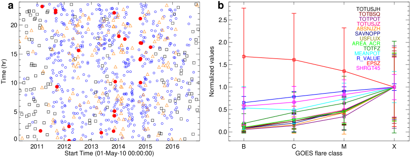
Figure 1: Properties of 845 flaring AR samples. (a) Distribution of flare start time in GOES 1–8 Å. B-, C-, M-, and X-class AR samples are denoted as black square, blue circle, orange triangle, and red filled circle, respectively. (b) Mean value (with 1$\sigma$ error bar) of SDO/HMI magnetic parameter normalized to that of the X-class vs. the class of AR samples; also see Table 1.

In Figure 1(a) we plot the distribution of the flare start time in GOES 1–8 Å of all the AR samples, which shows a semi-homogeneous spread within a 24 hr time period. Therefore, in this study we retrieve the values of the 13 HMI predictive parameters for each AR in our database at the time of the beginning of its flare date (mostly at 00:12 UT), using the routine ssw_jsoc_time2data from the SolarSoft package. Since flares originated from our sample ARs can occur anytime within a one day period as shown above, choosing AR parameter values measured at the beginning of the flare date for all samples is in accordance with our objective of predicting flares within 24 hours.

Table 2: Spearman Correlation Coefficients $\rho$ among AR Class and 13 SDO/HMI Magnetic Parameters

	TOT	TOT	TOT	TOT	ABS	SAVN	US	AREA	TOT	MEAN	R_		SHR
	USJH	BSQ	POT	USJZ	NJZH	CPP	FLUX	_ACR	FZ	POT	VALUE	EPSZ	GT45
TOTUSJH	1	0.95	0.93	0.99	0.69	0.75	0.96	0.94	0.64	0.51	0.9	$-$0.11	0.42
TOTBSQ	0.95	1	0.94	0.93	0.61	0.67	0.97	0.93	0.7	0.53	0.84	$-$0.08	0.38
TOTPOT	0.93	0.94	1	0.91	0.66	0.68	0.9	0.89	0.53	0.74	0.88	$-$0.26	0.63
TOTUSJZ	0.99	0.93	0.91	1	0.67	0.74	0.96	0.94	0.61	0.46	0.86	$-$0.13	0.42
ABSNJZH	0.69	0.61	0.66	0.67	1	0.86	0.6	0.6	0.31	0.5	0.68	$-$0.21	0.44
SAVNCPP	0.75	0.67	0.68	0.74	0.86	1	0.67	0.69	0.38	0.43	0.72	$-$0.17	0.37
USFLUX	0.96	0.97	0.9	0.96	0.6	0.67	1	0.92	0.76	0.42	0.83	0.03	0.29
AREA_ACR	0.94	0.93	0.89	0.94	0.6	0.69	0.92	1	0.55	0.48	0.79	$-$0.22	0.4
TOTFZ	0.64	0.7	0.53	0.61	0.31	0.38	0.76	0.55	1	0.01	0.53	0.61	$-$0.18
MEANPOT	0.51	0.53	0.74	0.46	0.5	0.43	0.42	0.48	0.04	1	0.63	$-$0.52	0.86
R_VALUE	0.9	0.84	0.88	0.86	0.68	0.72	0.83	0.79	0.53	0.63	1	$-$0.16	0.51
EPSZ	$-$0.11	$-$0.08	$-$0.26	$-$0.13	$-$0.21	$-$0.17	0.03	$-$0.22	0.61	$-$0.52	$-$0.16	1	$-$0.68
SHRGT45	0.42	0.38	0.63	0.42	0.44	0.37	0.29	0.4	-0.18	0.86	0.51	$-$0.68	1
AR Class	0.74	0.68	0.67	0.74	0.59	0.64	0.68	0.68	0.4	0.39	0.71	-0.16	0.33

We further make some exploratory data analyses of our AR samples. First, we compare the magnitude (mean plus/minus 1$\sigma$) of the predictive parameters with AR classes in Table 1 and Figure 1(b). It appears that ranging from the B to X class, almost all parameters exhibit a monotonic change of the mean values, with a Pearson correlation coefficient of $\sim$0.78–0.98. This indicates that ARs producing higher GOES class flares tend to possess larger values of these physical parameters. However, it is also clear that these property values of ARs with different classes could overlap with each other significantly, as the fluctuations in many cases are almost comparable with the means. Thus it is impractical to forecast flares with multiple classes simply based on magnitudes of these quantities. Second, we analyze the correlations $\rho$ among the magnetic parameters and AR classes using Spearman’s rank correlation method. The result in Table 2 shows that the AR class is strongly correlated with 9 out of 13 magnetic parameters (with $\rho\gtrsim 0.6$), while it is weakly correlated with the remaining four parameters (with $0.4\gtrsim|\rho|\gtrsim 0.2$). This implies that these parameters could potentially have good classifying capability of ARs. We also note that there are strong correlations between some parameters, such as TOTUSJH and TOTUSJZ; nevertheless, predicting variables with a high correlation still could be complementary features (e.g., Guyon & Elisseeff, 2003).

3 METHODOLOGY

We resort to RF, an inherent multi-class classifier, to perform flare prediction. RF is a general term for the random decision forests, an ensemble learning technique mainly for classification and regression tasks (Breiman, 2001). In the training phase, it constructs a collection of decision trees (i.e., tree-like predictive models), each of which is grown based on training records selected using the bagging method (i.e., sampling with replacement), and on randomly selected features when splitting each node. In the testing phase, an unknown sample is evaluated by all decision tress, and the RF outputs the class by majority votes (in the case of classification) or yields the mean prediction of trees (in the case of regression). Explicitly, the general scheme of RF operates as follows.

1. Training: Given a training data set $D=d_{1},...,d_{n}$ with responses $R=r_{1},...,r_{n}$, a total of $M$ trees are grown, each of which is built using the following algorithm:

   1. Randomly sample, with replacement, $n$ times to form a training set $(D_{m},R_{m})$.

   2. A decision or regression tree $T_{m}$ on $(D_{m},R_{m})$ is trained. At each node split, $f$ variables (predictive parameters) are randomly sampled, and the best split is determined based on information gain or the Gini impurity measure (Gini importance or the mean decrease Gini). By default, $f=\sqrt{F}$ for classification and $f=\frac{F}{3}$ for regression, where $F$ is the total number of variables.

2. Testing/validation: For an unknown sample data record $d^{\prime}$, forecasting can be made by taking the majority vote for classification decision trees, or can be given by $\frac{1}{M}\sum_{m=1}^{M}T_{m}(d^{\prime})$ for regression trees.

For our flare prediction, we run RF in the classification mode. In the training phase, each input training sample contains the 13 SHARP parameter values of an AR and its corresponding maximum GOES flare class. In the testing/validation phase, the 13 SHARP parameters of an AR sample are used as the model input, and the RF classifier predicts the maximum GOES class of this AR. We note that the ERT method used by Nishizuka et al. (2017) randomizes, rather than optimizes as what RF does, the splits on trees. A full comparison of these two algorithms is out of the scope of this paper (see Geurts et al., 2006).

It can be noticed that in our database, there are more C-class AR samples (552) while less X-class samples (23), compared to M-class (142) and B-class (128) samples. In order to alleviate the class imbalance issue that poses a major challenge in machine learning (e.g., Japkowicz & Stephen, 2002), we randomly select 142 unique C-class ARs from their total 552 samples to form a complete data set. To avoid any bias, we repeat this random selection 100 times, so we end up with 100 data sets for multi-class classification, each consisting of 128 B-class, 142 C-class, 142 M-class, and 23 X-class AR samples. We also construct another kind of 100 data sets for binary class prediction, so as to facilitate comparisons with previous work. In doing so, we combine the B- and C-class (M- and X-class) to form the B/C (M/X) class, and randomly select (for 100 times) 165 unique B/C-class AR samples to couple with the 165 M/X-class samples.

In evaluating the performance of the RF classifier, we apply the commonly used 10-fold cross validation (CV) method. For each of the data set, we perform a stratified 10-fold partitioning using the function createFolds in the caret package (Kuhn, 2008) in R. That is, we divide all the samples into 10 groups of nearly equal sizes, which have balanced distributions of AR classes. The prediction function of RF is then trained using nine folds of data, and the one fold left out is used for validation. To account for the random error associated with each 10-fold CV, the CV procedure is repeated 100 times. The average of the total 10⁴ iterations (100 CVs for each of the 100 data sets for multi-class or binary classification) yields the final results.

To further characterize the prediction results, we consider a confusion matrix, a.k.a. a contingency table for each AR class k. The class k ARs correctly predicted as class k are called true positives (TP), and in case of wrong predictions, they are false negatives (FN). The ARs not in class k correctly predicted not as class k are true negatives (TN); otherwise they are false positives (FP) if predicted as class k. Using these quantities, we compute a various of standard performance metrics. They include recall (a.k.a. sensitive) $=\frac{{\rm TP}}{{\rm TP}+{\rm FN}}$, precision $=\frac{{\rm TP}}{{\rm TP}+{\rm FP}}$, accuracy $=\frac{{\rm TP}+{\rm TN}}{{\rm TP}+{\rm FP}+{\rm TN}+{\rm FN}}$, and the true skill statistics (TSS; Hanssen & Kuipers, 1965) defined as

$${\rm TSS}=\frac{{\rm TP}}{{\rm TP}+{\rm FN}}-\frac{{\rm FP}}{{\rm FP}+{\rm TN}}\ .$$ (1)

All these metrics have a value of 1 for perfect forecasts, and are used together for a comprehensive assessment. Because of its unbiasness over class-imbalance ratio (Woodcock, 1976), we follow the suggestion of Bloomfield et al. (2012) to mainly use the TSS score, which is the recall subtracted by the false alarm rate, when comparing our results with other flare forecasting studies.

4 RESULTS AND DISCUSSIONS

The RF algorithm was originally written in FORTRAN¹. Here we employ the application of RF using the function randomforest (Liaw & Wiener, 2002) in R. The function takes in a formula (i.e., combination of predictive parameters) and a training data set, as well as other optional arguments. Two important arguments are ntree, which defines the number of trees to be built for the ensemble, and mtry, which is the number of variables sampled at each node for splitting. Using one sample data set with the four AR classes (the selected C-class ARs are marked in Table 5), we tune these arguments using the tune function in the R package e1071 (Meyer et al., 2017), and find that setting ntree $=1000$ and mtry $=6$ usually produces results with slightly better accuracy than those computed with the default argument values (ntree $=500$ and mtry $=\sqrt{F}=3$ in our case). In general, the choice of the mtry argument has little impact on the accuracy of RF predictions (e.g., Liaw & Wiener, 2002). For demonstration purpose, a sample representative RF tree, created using the R package reprtree (Dasgupta, 2014), is portrayed in Figure 3 in appendix.

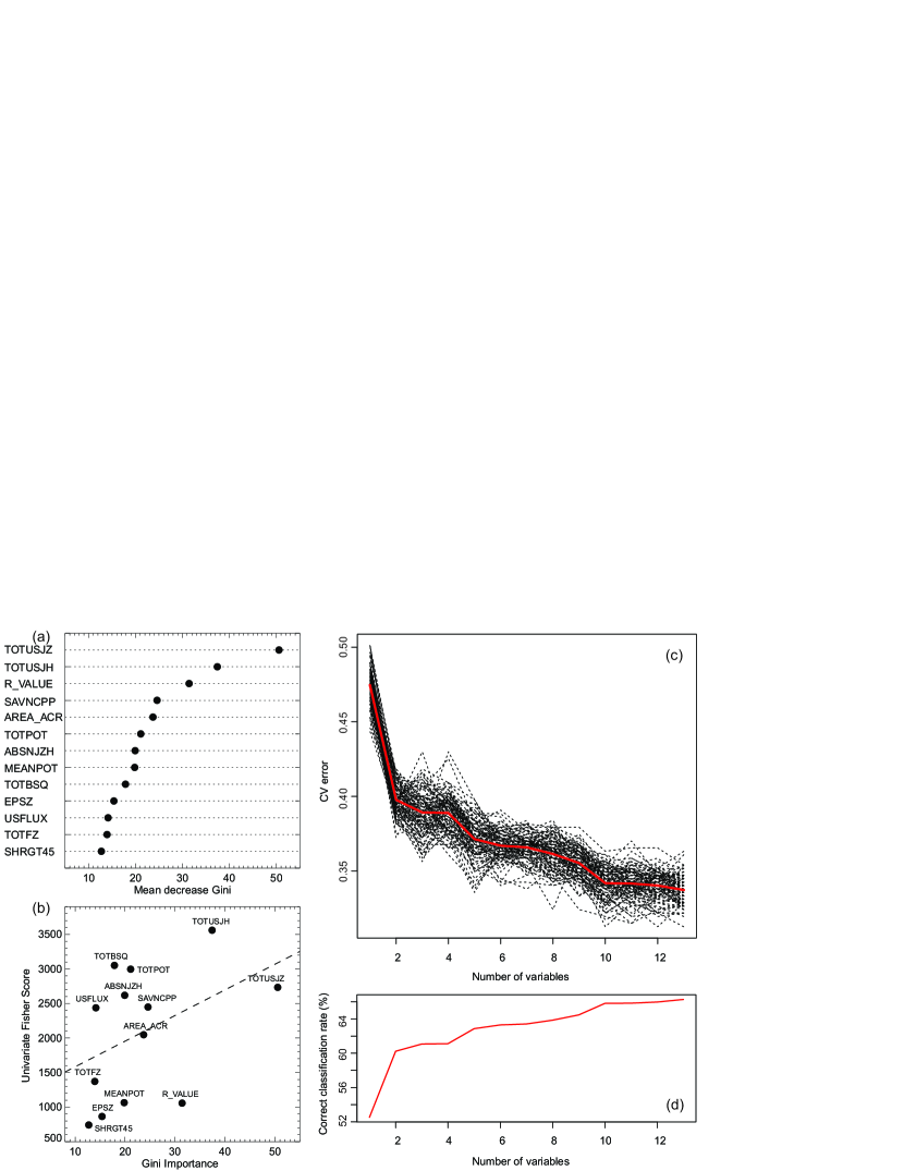
Figure 2: Magnetic parameter importance. (a) The Gini importance of the 13 SDO/HMI magnetic parameters for predicting flaring AR classes using the RF method. (b) Univariate Fisher score calculated by Bobra & Couvidat (2015) vs. Gini importance from RF. The Pearson correlation coefficient is 0.42. The dashed line is a linear fit to the data. (c) 10-fold CV error vs. number of parameters used, showing the result from each of 100 iterations (black dotted line) and average of the 100 iterations (red thick line). (d) Averaged correct classification rate vs. number of parameters used, based on 100 iterations of the 10-fold CV.

4.1 Parameter Importance

As suggested by Bobra & Couvidat (2015), the 13 SDO/HMI magnetic parameters listed in Table 1 are most useful for discriminating flaring from non-flaring ARs. A natural question is: what is the relative importance of these parameters in classifying flaring ARs into B-, M-, C-, and X-class? An advantage of the RF method is that it can rank the importance of predictive variables by measuring their impacts on accuracy or Gini impurity when splitting nodes (Breiman, 2001). A larger value of Gini importance means that this particular variable plays a greater role in partitioning data into the defined classes. Using the same data set as above, the randomForest function generates the Gini importance (mean decrease Gini) of the magnetic parameters as illustrated in Figure 2(a) and also listed in Table 1. The result shows that the order of parameter importance is generally consistent with the correlations of parameters with the AR class (Table 2), with the total unsigned vertical current (TOTUSJZ), the total unsigned current helicity (TOTUSJH), and the total unsigned flux around high-gradient AR polarity inversion lines (R_VALUE) being among the most important parameters. We caution that due to the randomness associated with RF (random trees and randomly sampled predictors at each node), different iterations may produce different results, but the order of the most important predictors remains relatively stable. In any case, the parameter rank determined by Gini importance in RF only roughly agrees with that determined by the univariate Fisher score (Bobra & Couvidat, 2015). Figure 2(b) presents a scatter plot of these two quantities for the 13 parameters, showing a weak to moderate Pearson correlation with a coefficient of $\sim$0.42. One parameter of interest is R_VALUE, which has a relatively low univariate score but a quite high Gini importance. The R_VALUE parameter was shown to be effective in forecasting major flares (Schrijver, 2007; Welsch et al., 2009). Our result supports this view and connotes that it could also help classifying flaring ARs into different classes. Lastly, we reiterate that the Gini importance derived here is for the purpose of classifying multi-class ARs, different from that of the univariate score of Bobra & Couvidat (2015) that is to distinguish between flaring and non-flaring ARs.

Based on the variable importance, the function rfcv in the randomForest package can perform automatic variable selections, by sequentially removing the least important variable(s) and performing the nested cross-validated model prediction. We show in Figure 2(c) and Figure 2(d) the error of 10-fold CV (repeated 100 times) and the averaged correct classification rate, respectively, against the number of SDO/HMI parameters used at each step. It suggests that the optimal model, with an error rate of $\sim$0.34 and an equivalent overall correct classification rate of $\sim$66%, can be achieved for this data set when all 13 variables are used. Similar results are obtained when using other multi-class data sets we constructed. Thus, no further feature selection is carried out, and below we use all the 13 SDO/HMI parameters as input variables of the RF model.

4.2 Flare Prediction using 13 SDO/HMI Parameters and RF

In this subsection, we describe the flare prediction results using the RF algorithm, and compare with previous studies of flare forecasting for a 24 hrs time interval. Using different kinds of flaring AR data sets we prepared, we carry out two experiments, the main one⁴ for multi-class classification (i.e., B-, C-, M-, and X-class ARs) and an additional one for binary classification (i.e., B/C- and M/X-class ARs). The latter is analogous to forecasting flares larger than a certain class (here M1.0 class), which is the approach of most previous studies. For each experiment, as we described earlier we obtain the final results based on the average of 100 times 10-fold CVs on each of the 100 AR samples. The TSS score is used as the standard measure for results comparison, while other metrics are also considered.

Table 3: RF Multi-class Flare Prediction Results (within 24 hrs) using 13 SDO/HMI Parameters and Comparison to Other Studies

Prediction$\downarrow$ Observation$\rightarrow$	B Class (n=128)	C Class (n=142)	M Class (n=142)	X Class (n=23)
B Class	103.980$\pm$3.624	33.413$\pm$4.287	10.467$\pm$1.770	0.000$\pm$0.000
C Class	23.187$\pm$3.569	74.700$\pm$5.685	33.984$\pm$3.724	0.884$\pm$0.492
M Class	0.833$\pm$0.839	33.866$\pm$4.259	95.237$\pm$3.703	15.296$\pm$0.939
X Class	0.000$\pm$0.000	0.021$\pm$0.144	2.312$\pm$1.294	6.819$\pm$0.804
Recall
This work	0.812$\pm$0.039	0.526$\pm$0.050	0.671$\pm$0.037	0.297$\pm$0.039
Yuan et al. (2010)	0.714	0.138	0.221	0.206
Bloomfield et al. (2012)	N/A	0.737	0.693	0.859
Precision
This work	0.703$\pm$0.037	0.563$\pm$0.054	0.656$\pm$0.036	0.745$\pm$0.152
Yuan et al. (2010)	0.763	0.529	0.357	0.438
Bloomfield et al. (2012)	N/A	0.330	0.136	0.029
Accuracy
This work	0.844$\pm$0.017	0.712$\pm$0.026	0.778$\pm$0.019	0.957$\pm$0.005
Yuan et al. (2010)	0.861	0.722	0.652	0.843
Bloomfield et al. (2012)	N/A	0.711	0.829	0.881
TSS
This work	0.669$\pm$0.039	0.328$\pm$0.050	0.500$\pm$0.037	0.291$\pm$0.039
Yuan et al. (2010)	0.630	0.090	0.054	0.160
Bloomfield et al. (2012)	N/A	0.443	0.526	0.740

Table 4: RF Binary-class Flare Prediction Results (within 24 hrs) using 13 SDO/HMI Parameters and Comparison to Other Studies

Prediction$\downarrow$ Observation$\rightarrow$	B/C Class (n=165)	M/X Class (n=165)
B/C Class	129.536$\pm$4.025	41.722$\pm$3.370
M/X Class	35.464$\pm$4.025	123.278$\pm$3.370
Recall
This work	0.785$\pm$0.036	0.747$\pm$0.030
Bloomfield et al. (2012)	N/A	0.704
Ahmed et al. (2013)	N/A	0.523
Bobra & Couvidat (2015)	N/A	0.832$\pm$0.042
Nishizuka et al. (2017)	N/A	0.716
Precision
This work	0.756$\pm$0.033	0.777$\pm$0.033
Bloomfield et al. (2012)	N/A	0.146
Ahmed et al. (2013)	N/A	0.740
Bobra & Couvidat (2015)	N/A	0.417$\pm$0.037
Nishizuka et al. (2017)	N/A	0.969
Accuracy
This work	0.766$\pm$0.023	0.766$\pm$0.021
Bloomfield et al. (2012)	N/A	0.830
Ahmed et al. (2013)	N/A	0.963
Bobra & Couvidat (2015)	N/A	0.924$\pm$0.007
Nishizuka et al. (2017)	N/A	0.990
TSS
This work	0.532$\pm$0.036	0.532$\pm$0.030
Bloomfield et al. (2012)	N/A	0.539
Ahmed et al. (2013)	N/A	0.512
Bobra & Couvidat (2015)	N/A	0.761$\pm$0.039
Nishizuka et al. (2017)	N/A	0.71$\pm$0.002

First, we apply RF to predict flaring ARs with four different classes. Detailed results including a confusion matrix and model performance metrics are presented in Table 3. It can be seen that the RF method works reasonably well in terms of recall, precision, and accuracy, except for a low recall of X-class ($\sim$0.30). A closer look reveals that the RF has difficulties in distinguishing X- from M-class AR samples. This is presumably due to the sparsity of the current X-class samples available for training, as the solar cycle 24 contemporaneous with SDO/HMI measurements is unusually quiet compared to previous cycles. Nevertheless, our TSS scores (about 0.67 for B class, 0.33 for C class, 0.50 for M class, and 0.29 for X class) outperform Yuan et al. (2010) in every AR class; in particular, we obtain a $\sim$10 times higher TSS score for the M class. Compared to Bloomfield et al. (2012) which used solar cycles 21 and 22 observations for training, our TSS scores of the C- and M-classes are roughly similar while that of the X-class is $\sim$2.5 times lower. However, it can be noted that the precision of X-class of Bloomfield et al. (2012) is very low (due to a large number of FP counts), about 26 times lower than ours, while at the mean time, their recall of the X-class is only about 3 times better. We recognize that recall is a very important metric especially for the most energetic X-class ARs/flares, as a miss is usually deemed worse than a false alarm. It could be expected that provided with more X-class training samples, our method may yield improved recall performance while maintaining a high precision prediction for X-class ARs.

Second, we make binary predictions and show the confusion matrix and performance metrics in Table 4. We also compare our results with previous works on forecasting flares larger than M1.0 class. By looking at the TSS score, it is apparent that the performance of our method coupling SDO/HMI magnetic parameters with RF (TSS $\approx 0.53$) is very similar to Bloomfield et al. (2012) and Ahmed et al. (2013), while being $\sim$28% lower than Bobra & Couvidat (2015) and Nishizuka et al. (2017). Nonetheless, we obtain quite high scores in both recall and precision. We note that Nishizuka et al. (2017) used the ERT classifier similar to RF, and also considered, besides magnetic field parameters, UV brightenings and previous flare activity to achieve high metric scores.

It is worth noting that all our training AR samples are flare productive, with the AR classes defined in the same way as Yuan et al. (2010) (see Section 2). Many previous studies (e.g., Ahmed et al., 2013; Bobra & Couvidat, 2015; Nishizuka et al., 2017) include non-flaring ARs as negative samples. This difference in building data sets with multiple classes may affect the performance comparisons. For example, the database for our binary classification is constructed from multi-class AR samples. As a result, the RF classifier actually works to distinguish M/X-class ARs from B/C-class ARs ($\sim$80% are C-class ARs in our data sets). Thus intuitively, including non-flaring AR samples might facilitate/improve our prediction. The ideal situation would be to conduct performance comparisons between different flare forecasting methods from the same database (Barnes & Leka, 2008).

5 SUMMARY AND DISCUSSIONS

Although not based on physical models of flares, solar flare prediction taking advantage of modern machine learning techniques has drawn significant attention in recent years. What distinguishes the present work from previous studies is the use of prediction parameters from the state-of-the-art SDO/HMI instrument and the advanced RF algorithm, with the main goal of multi-class flare forecasting. Based on flare events that occur from 2010 May to 2016 December, we build a database containing sample ARs that belong to four classes (B, C, M, and X), stipulated according to the maximum GOES class of flare(s) that an AR ever produces. We then apply the RF classifier to make flare predictions in 24 hours, evaluate the model performance using the 10-fold CV technique, and characterize our results and make comparisons with previous studies using performance metrics. The main results are summarized as follows.

1. From the evaluation of variable importance by the RF algorithm, the 13 SDO/HMI magnetic parameters used by Bobra & Couvidat (2015) to discriminate flaring and non-flaring ARs are also helpful in distinguishing flaring ARs into four different classes, yet the orders of parameter importance determined from these two approaches only roughly agree, with a weak to moderate Pearson correlation of $\sim$0.42. The three most important parameters for classifying ARs are TOTUSJZ, TOTUSJH, and R_VALUE. We surmise that the ranking of one parameter versus another is not really as significant as using all 13 parameters in combination.

2. In classifying flaring ARs into multiple classes, we achieve a TSS score of about 0.70, 0.33, 0.50, and 0.29 for B-, C-, M-, and X-class ARs, respectively, which clearly outperform Yuan et al. (2010) that used the same way for defining AR samples. Our TSS scores of C and M classes are roughly comparable to those of Bloomfield et al. (2012), but that of the X class is $\sim$2.5 times lower, most probably due to the lack of X-class training samples in the solar cycle 24. In forecasting flares larger than M1.0 class, our method yields a TSS score of $\sim$0.53, comparable to Bloomfield et al. (2012) and Ahmed et al. (2013), while being $\sim$28% lower than Bobra & Couvidat (2015) and Nishizuka et al. (2017). In general, we obtain fairly good scores in recall and precision at the same time.

It should be noted that (1) these result comparisons could be affected by the fact that the sample classes in the present study are defined using different criteria from many previous studies, and we consider flaring ARs only without including non-flaring AR regions. (2) To better train the random forest model for the main objective of multi-class classification, we randomly select C-class samples from a larger pool to construct training data with more balanced AR classes. Indeed, if we use the originally obtained 845 AR samples without undersampling the C class, the resulted TSS scores after 100 times of CVs are 0.411$\pm$0.023, 0.366$\pm$0.011, 0.341$\pm$0.021, and 0.268$\pm$0.025 for the B, C, M, and X class, respectively, much inferior to those in Table 3 except for the C class. Then the question is whether the model developed with the undersampled C class data can perform equally well for test data with original class ratios. To answer this, we revise the main experiment in Section 4.2 as follows. After randomly selecting 142 unique C-class ARs from the total of 552 C-class samples to form a complete data set with samples in other classes, we keep the leftover 410 C-class samples; when carrying out the 10-fold CVs, the data for validation also includes one fold from the 410 C-class data. In doing so, we build the model with undersampled C-class data (same as the previous main experiment) but validate it using data that reflects the original class ratios. The TSS scores obtained this way are 0.620$\pm$0.039, 0.333$\pm$0.028, 0.463$\pm$0.036, and 0.294$\pm$0.039 for the B, C, M, and X class, respectively, very similar to those in Table 3 (with difference only up to $\sim$7%). All these show that for this study, using data with more balanced classes can help build the optimal model, which can also perform well in an operational setting.

Based on all our experiments, we conclude that using SDO/HMI magnetic parameters and the RF algorithm is a valid method for flare forecasting. Importantly, incorporating other features of flaring ARs, such as previous flare activity, could be critical in improving the prediction performance (Nishizuka et al., 2017). Extended studies should also be made on multi-class flare forecasting using ERT, as it could be more computationally efficient and robust compared to RF. Related to multi-class classification, it will also be interesting to find out the most useful parameter for predicting a certain flare class. Another possible future work is to calculate the flare index (Abramenko, 2005) for each AR, which can reflect the overall flare productivity by taking into account the numbers of flares of different GOES classes within a certain time period; then the RF/ERT classifier can be run in the regression mode to predict the flare index quantitatively. More generally, as solar data from various instruments are growing rapidly, including such as those from SDO and the recently digitized historical ground-based H-alpha images covering many solar cycles (Liu et al., 2010), the RF/ERT algorithms may be helpful in solving other multi-class problems in solar physics.

Table 5: 845 Samples of Flaring ARs

Start Time	NOAA	GOES	Start Time	NOAA	GOES	Start Time	NOAA	GOES
YY/MM/DD UT	AR	Class	YY/MM/DD UT	AR	Class	YY/MM/DD UT	AR	Class
11/02/15 01:44	11158	X2.2	11/03/09 23:13	11166	X1.5	11/09/06 22:12	11283	X2.1
11/09/07 22:32	11283	X1.8	11/09/24 09:21	11302	X1.9	12/03/05 02:30	11429	X1.1
12/03/07 00:02	11429	X5.4	12/07/12 15:37	11520	X1.4	13/05/15 01:25	11748	X1.2
13/10/28 01:41	11875	X1.0	13/11/05 22:07	11890	X3.3	13/11/08 04:20	11890	X1.1
13/11/10 05:08	11890	X1.1	13/11/19 10:14	11893	X1.0	14/01/07 18:04	11944	X1.2
14/03/29 17:35	12017	X1.0	14/10/22 14:02	12192	X1.6	14/10/25 16:55	12192	X1.0
14/10/26 10:04	12192	X2.0	14/10/27 14:12	12192	X2.0	14/10/24 21:07	12192	X3.1
14/11/07 16:53	12205	X1.6	15/03/11 16:11	12297	X2.2	10/05/05 17:13	11069	M1.2
10/06/12 00:30	11081	M2.0	10/08/07 17:55	11093	M1.0	10/10/16 19:07	11112	M2.9
10/11/06 15:27	11121	M5.4	11/03/07 09:14	11164	M1.8	11/03/07 19:43	11165	M3.7
11/03/14 19:30	11169	M4.2	11/03/24 12:01	11176	M1.0	11/06/07 06:16	11226	M2.5
11/07/27 15:48	11260	M1.1	11/08/03 03:08	11261	M1.1	11/08/04 03:41	11261	M9.3
11/09/23 01:47	11295	M1.6	11/09/30 18:55	11305	M1.0	11/10/01 08:56	11305	M1.2
11/10/02 00:37	11305	M3.9	11/12/25 18:11	11380	M4.0	11/12/26 02:13	11380	M1.5
12/02/06 19:31	11410	M1.0	12/03/14 15:08	11432	M2.8	12/03/15 07:23	11432	M1.8
12/03/17 20:32	11434	M1.4	12/04/27 08:15	11466	M1.0	12/05/07 14:03	11471	M1.9
12/05/08 13:02	11476	M1.4	12/05/09 14:02	11476	M1.8	12/05/10 04:11	11476	M5.7
12/05/06 17:41	11476	M1.3	12/06/06 19:54	11494	M2.1	12/06/14 12:52	11504	M1.9
12/07/04 16:33	11513	M1.8	12/07/06 13:26	11513	M1.2	12/07/02 19:59	11515	M3.8
12/07/04 14:35	11515	M1.3	12/07/05 20:09	11515	M1.6	12/07/06 18:48	11515	M1.3
12/07/07 10:57	11515	M2.6	12/07/29 06:15	11532	M2.3	12/07/30 15:39	11532	M1.1
12/07/28 20:44	11532	M6.1	12/08/18 00:24	11543	M5.5	12/09/09 21:50	11564	M1.2
12/11/20 19:21	11618	M1.6	12/11/21 06:45	11618	M1.4	12/11/27 21:05	11620	M1.0
12/11/28 21:20	11620	M2.2	13/01/11 14:51	11654	M1.0	13/02/17 15:45	11675	M1.9
13/03/05 07:47	11686	M1.2	13/03/15 05:46	11692	M1.1	13/04/11 06:55	11719	M6.5
13/05/02 04:58	11731	M1.1	13/05/03 16:39	11731	M1.3	13/05/05 17:42	11734	M1.4
13/05/31 19:52	11760	M1.0	13/06/05 08:14	11762	M1.3	13/06/23 20:48	11778	M2.9
13/08/12 10:21	11817	M1.5	13/08/17 18:49	11818	M1.4	13/10/24 10:30	11877	M3.5
13/10/28 04:32	11877	M5.1	13/10/26 19:49	11882	M1.0	13/10/28 15:07	11882	M4.4
13/10/25 20:54	11882	M1.9	13/11/01 19:46	11884	M6.3	13/11/02 22:13	11884	M1.6
13/11/03 05:16	11884	M4.9	13/11/08 09:22	11891	M2.3	13/11/15 02:20	11899	M1.0
13/11/23 12:49	11899	M1.0	13/12/07 07:17	11909	M1.2	13/12/22 21:23	11928	M1.6
13/12/29 07:49	11936	M3.1	13/12/31 21:45	11936	M6.4	14/01/01 18:40	11936	M9.9
14/01/07 03:49	11946	M1.0	14/02/01 07:14	11967	M3.0	14/02/02 09:24	11967	M4.4
14/02/04 15:25	11967	M1.5	14/02/07 04:47	11967	M2.0	14/02/02 06:24	11968	M2.6
14/02/04 01:16	11968	M3.8	14/02/07 10:25	11968	M1.9	14/02/11 16:34	11974	M1.8
14/02/12 06:54	11974	M2.3	14/02/13 15:45	11974	M1.4	14/02/14 16:33	11974	M1.0
14/02/16 09:20	11977	M1.2	14/02/20 07:26	11982	M3.0	14/02/28 00:44	11991	M1.1
14/03/05 02:06	11991	M1.0	14/03/10 22:45	11996	M1.4	14/03/11 03:44	11996	M3.5
14/03/09 20:13	12002	M1.0	14/03/10 15:21	12002	M1.7	14/04/16 19:54	12035	M1.0
14/06/03 03:58	12077	M1.4	14/06/12 09:23	12085	M1.8	14/06/12 19:56	12089	M1.1
14/07/08 16:06	12113	M6.5	14/10/09 06:48	12182	M1.2	14/12/01 06:26	12222	M1.8
14/12/04 08:00	12222	M1.3	14/12/17 18:54	12241	M1.4	14/12/18 21:41	12241	M6.9
14/12/27 02:03	12249	M2.2	15/01/03 09:40	12253	M1.1	15/01/04 15:18	12253	M1.3
15/01/28 04:21	12268	M1.4	15/01/29 11:32	12268	M2.1	15/01/30 05:29	12277	M1.7
15/02/04 02:08	12277	M1.2	15/02/09 22:19	12280	M2.4	15/04/08 14:37	12320	M1.4
15/05/05 17:12	12335	M2.6	15/06/21 18:10	12367	M1.1	15/06/20 06:28	12371	M1.0
15/06/21 01:02	12371	M2.0	15/06/22 17:39	12371	M6.6	15/06/25 08:02	12371	M7.9
15/07/03 12:47	12378	M1.5	15/07/06 20:32	12381	M1.7	15/08/21 19:10	12403	M1.1
15/08/22 21:19	12403	M3.5	15/08/24 07:26	12403	M5.6	15/08/27 04:48	12403	M2.9
15/08/28 13:04	12403	M2.2	15/09/17 09:34	12415	M1.1	15/09/20 17:32	12415	M2.1
15/10/01 13:03	12422	M4.5	15/10/16 06:11	12434	M1.1	15/10/15 23:27	12434	M1.1
15/10/31 17:48	12443	M1.0	15/11/04 13:31	12443	M3.7	15/11/09 12:49	12449	M3.9
15/12/23 00:23	12473	M4.7	16/02/13 15:16	12497	M1.8	16/02/14 19:18	12497	M1.0
16/02/15 10:41	12497	M1.2	16/04/18 00:14	12529	M6.7	16/11/29 23:29	12615	M1.2
10/07/13 10:43	11087	C2.6	10/08/01 07:55	11092	C3.2	10/09/06 14:54	11105	C2.5∗
10/10/27 16:59	11117	C1.2	10/10/31 03:13	11117	C1.8	10/10/26 08:09	11119	C1.0
10/11/15 07:28	11124	C2.3	10/12/14 15:03	11133	C2.3∗	11/01/03 23:26	11142	C1.1
11/03/27 23:18	11181	C1.0	11/04/18 18:55	11193	C1.5	11/04/29 20:40	11199	C1.8∗
11/05/15 14:11	11208	C1.3	11/05/09 17:31	11210	C1.5	11/06/15 14:19	11234	C3.2
11/06/17 23:37	11234	C3.9	11/06/19 16:03	11237	C1.5∗	11/07/07 02:31	11243	C1.0
11/07/03 10:54	11244	C2.1	11/07/08 14:56	11247	C2.3∗	11/07/11 10:47	11247	C2.6
11/07/12 14:44	11247	C1.9	11/07/18 10:19	11254	C1.0	11/07/30 12:11	11265	C1.3
11/07/31 19:01	11265	C1.7	11/08/09 13:29	11266	C2.2	11/08/05 05:56	11267	C1.3
11/08/06 11:41	11267	C1.3	11/08/07 08:24	11267	C1.6	11/08/18 14:59	11271	C1.1
11/08/20 22:54	11271	C2.9∗	11/08/24 16:31	11271	C1.1	11/08/26 03:29	11271	C1.0∗
11/08/17 16:16	11272	C2.6	11/08/18 06:40	11272	C1.2	11/08/21 18:15	11272	C1.5
11/08/30 03:06	11274	C1.9	11/09/03 03:19	11280	C1.0	11/08/30 22:02	11281	C5.5
11/09/02 15:09	11281	C1.8∗	11/09/03 13:57	11281	C1.0∗	11/09/08 18:26	11289	C2.5
11/09/16 22:09	11290	C1.4∗	11/09/14 20:42	11297	C9.2	11/09/15 21:09	11297	C2.6∗
11/09/16 08:42	11297	C2.2∗	11/09/20 06:44	11301	C2.0∗	11/09/21 11:17	11301	C3.9
11/10/07 01:14	11313	C1.2∗	11/10/10 14:30	11313	C4.5∗	11/10/11 23:19	11316	C1.1
11/10/12 09:46	11316	C1.7	11/10/14 15:09	11316	C1.1	11/10/15 18:13	11316	C1.5
11/10/16 13:51	11317	C1.4	11/10/22 15:14	11324	C4.1	11/10/28 11:48	11324	C1.7
11/10/30 09:24	11330	C2.4	11/11/16 23:40	11346	C5.0	11/11/17 07:16	11346	C6.0
11/11/18 16:38	11346	C1.1∗	11/11/17 13:53	11352	C3.1	11/11/18 17:07	11354	C2.7∗
11/11/19 11:19	11354	C1.4	11/11/20 16:35	11354	C6.1	11/11/22 00:33	11354	C1.2
11/11/26 17:12	11358	C1.0	11/11/27 11:59	11358	C1.1∗	11/11/25 21:49	11359	C2.4
11/11/28 18:22	11361	C3.2∗	11/11/29 03:25	11361	C2.1	11/12/01 20:27	11361	C1.1
11/12/05 03:09	11361	C1.9	11/11/29 08:54	11362	C2.5∗	11/12/05 06:35	11362	C1.4
11/12/03 05:48	11363	C1.2	11/12/05 23:20	11363	C6.9	11/12/07 15:34	11364	C1.3
11/12/09 13:05	11374	C3.1∗	11/12/10 23:00	11374	C1.0	11/12/12 08:30	11374	C1.2
11/12/17 22:47	11376	C3.2	11/12/18 04:59	11376	C1.8	11/12/20 22:38	11376	C6.2
11/12/21 20:08	11376	C1.5∗	11/12/22 01:56	11381	C5.4∗	11/12/27 04:11	11386	C8.9
11/12/28 20:18	11386	C4.0	11/12/31 17:17	11386	C1.2	12/01/10 22:34	11391	C1.7
12/01/13 06:01	11391	C2.2	12/01/08 06:08	11393	C1.9	12/01/09 10:31	11393	C1.1∗
12/01/10 01:49	11393	C1.0	12/01/09 20:01	11395	C2.6	12/01/11 11:04	11395	C1.6
12/01/12 00:49	11395	C1.5∗	12/01/14 03:19	11396	C2.1	12/01/19 12:41	11396	C3.2∗
12/02/08 21:48	11415	C2.9	12/02/19 08:41	11422	C1.0∗	12/03/01 15:10	11423	C3.4
12/03/03 03:01	11427	C1.3	12/03/04 17:24	11427	C3.2	12/03/08 02:49	11428	C7.2∗
12/03/10 06:53	11428	C1.9	12/03/21 13:54	11440	C1.2	12/04/04 16:17	11450	C1.2
12/04/05 20:49	11450	C1.5	12/04/18 16:54	11459	C5.2∗	12/04/21 20:10	11459	C1.8∗
12/04/22 21:05	11459	C1.7	12/04/19 00:00	11460	C1.4	12/04/21 01:27	11460	C2.4∗
12/04/23 17:38	11461	C2.0	12/04/18 14:51	11463	C5.9	12/04/19 02:54	11463	C2.9
12/04/20 22:25	11465	C1.4	12/04/22 21:42	11465	C2.4	12/04/27 10:53	11465	C2.4
12/04/27 13:18	11467	C2.0	12/04/28 21:48	11467	C1.1	12/04/27 01:59	11469	C1.0∗
12/04/28 08:54	11469	C1.7	12/04/29 14:27	11469	C1.1	12/05/02 20:38	11469	C1.9∗
12/05/03 16:39	11469	C2.3	12/05/04 04:48	11469	C1.3	12/05/19 12:04	11479	C1.0
12/05/14 19:22	11483	C1.8	12/05/16 00:14	11484	C1.8∗	12/05/23 00:15	11484	C1.2
12/05/24 19:57	11488	C3.9	12/05/27 04:42	11492	C3.1	12/06/12 05:47	11506	C1.0
12/06/11 18:59	11507	C1.5∗	12/06/12 16:01	11507	C1.4∗	12/06/25 20:55	11512	C1.4
12/06/27 07:57	11512	C3.2	12/06/28 04:45	11512	C4.2∗	12/06/29 18:35	11512	C1.1
12/07/27 03:58	11528	C5.0	12/08/01 12:47	11535	C2.3	12/08/03 21:20	11535	C3.0
12/08/04 06:03	11535	C1.3	12/08/09 05:27	11538	C3.2	12/08/08 16:10	11542	C1.9
12/08/09 22:42	11542	C1.4	12/08/10 18:38	11542	C1.4	12/08/11 16:28	11542	C2.0∗
12/08/14 22:23	11542	C1.6	12/09/01 19:39	11553	C1.9	12/09/02 13:37	11553	C1.1∗
12/08/25 02:24	11554	C1.7	12/08/30 04:48	11554	C1.5	12/08/31 19:45	11560	C8.4
12/09/02 18:00	11560	C5.5∗	12/09/03 16:30	11560	C1.3∗	12/09/05 16:14	11560	C1.1
12/09/06 03:11	11560	C1.8∗	12/09/07 17:05	11562	C1.3	12/09/11 08:25	11567	C1.1
12/09/09 14:51	11568	C1.7∗	12/09/11 01:00	11569	C3.5	12/09/25 06:34	11573	C1.0
12/09/20 11:27	11574	C1.0	12/09/25 04:24	11577	C3.6	12/10/10 21:40	11585	C1.5
12/10/17 00:44	11589	C1.1	12/10/19 05:10	11589	C1.9	12/10/23 07:40	11593	C3.0
12/10/19 18:42	11594	C1.7∗	12/10/21 02:54	11596	C7.8∗	12/10/26 10:23	11596	C1.5
12/11/14 13:35	11611	C4.3	12/11/14 23:33	11613	C1.3	12/11/15 20:14	11613	C1.0∗
12/11/14 13:22	11614	C1.3∗	12/11/29 11:13	11623	C2.0	12/12/18 16:37	11633	C1.3
12/12/23 05:43	11633	C1.3∗	13/01/01 08:47	11640	C1.2	13/01/12 21:57	11652	C3.1
13/01/13 18:30	11652	C2.3	13/01/14 01:15	11652	C6.5	13/01/31 04:30	11663	C1.1
13/02/05 08:12	11669	C6.3∗	13/02/06 05:53	11669	C1.0∗	13/02/12 17:47	11670	C1.5∗
13/03/12 22:42	11689	C3.6	13/03/14 05:45	11691	C2.1	13/03/19 13:50	11695	C1.5∗
13/03/13 16:15	11696	C1.4	13/03/15 15:09	11696	C1.0	13/03/16 08:30	11698	C1.5
13/04/03 18:34	11711	C1.7	13/04/07 16:49	11713	C1.6	13/04/08 15:42	11714	C1.6
13/04/06 23:31	11718	C1.0	13/04/07 15:55	11718	C3.1	13/04/09 13:28	11718	C1.5
13/04/10 17:56	11718	C3.4∗	13/04/11 16:52	11718	C1.0	13/04/13 19:46	11718	C1.4
13/04/10 12:54	11721	C1.2	13/04/11 10:09	11721	C4.2	13/04/15 13:58	11723	C1.3
13/04/16 07:30	11723	C1.3	13/04/20 22:46	11726	C1.3∗	13/04/21 19:59	11726	C2.7
13/04/23 23:21	11726	C2.5∗	13/04/24 22:39	11726	C1.6	13/04/30 20:43	11730	C2.6
13/05/01 07:23	11730	C5.5∗	13/04/29 19:26	11733	C4.0	13/05/05 19:57	11739	C8.3
13/05/06 01:58	11739	C2.4	13/05/10 16:30	11739	C2.5	13/05/11 02:52	11744	C1.3
13/05/17 04:37	11744	C5.0∗	13/05/13 21:58	11745	C8.3	13/05/21 10:23	11745	C1.2
13/05/19 21:11	11750	C4.7	13/05/20 00:41	11750	C4.0	13/05/18 06:32	11752	C1.3
13/05/23 12:26	11755	C1.3	13/05/25 20:17	11755	C1.6	13/05/21 22:32	11756	C2.9
13/05/22 19:46	11756	C2.4∗	13/05/23 18:41	11756	C3.4	13/05/24 16:31	11756	C2.1∗
13/06/10 14:18	11765	C1.9	13/06/19 11:49	11773	C1.5	13/06/22 17:31	11773	C1.5
13/06/17 04:29	11775	C1.0	13/06/18 06:48	11775	C2.2	13/06/19 07:20	11775	C3.5
13/06/20 15:55	11775	C1.4	13/06/24 20:35	11775	C3.0∗	13/06/19 16:46	11776	C1.0
13/06/21 18:02	11776	C1.0	13/06/30 16:44	11780	C2.0∗	13/06/29 16:01	11781	C1.1
13/07/06 17:31	11784	C1.1	13/07/04 05:20	11785	C3.9∗	13/07/05 21:30	11785	C3.5
13/07/06 08:07	11785	C1.0∗	13/07/07 12:05	11785	C1.7	13/07/09 13:25	11785	C2.3
13/07/11 09:04	11785	C1.0	13/07/13 05:36	11791	C1.4	13/07/15 16:55	11791	C1.0∗
13/07/16 10:10	11791	C1.9∗	13/07/17 01:49	11791	C1.1	13/07/20 03:34	11793	C2.1
13/07/21 08:24	11800	C3.1	13/07/24 18:13	11800	C1.0	13/07/25 22:37	11800	C2.1
13/07/27 12:28	11800	C1.0	13/07/28 19:57	11800	C1.6	13/07/30 01:10	11801	C1.1
13/08/21 03:36	11820	C1.3	13/08/22 19:08	11820	C1.5∗	13/08/23 06:42	11827	C1.1
13/08/21 07:25	11828	C2.2∗	13/08/22 20:23	11828	C1.4	13/09/01 14:16	11834	C1.7
13/09/03 17:26	11834	C1.3	13/08/30 02:04	11836	C8.3∗	13/08/31 17:20	11836	C2.6∗
13/09/04 21:31	11836	C1.3	13/09/05 19:46	11836	C1.5	13/09/04 08:36	11837	C2.6
13/09/05 21:59	11837	C1.4	13/09/24 22:50	11846	C1.1∗	13/09/29 05:11	11850	C1.7
13/10/04 03:17	11856	C2.5∗	13/10/07 15:34	11856	C2.3	13/10/10 16:40	11861	C1.3
13/10/11 22:56	11861	C6.3	13/10/12 22:02	11861	C2.9	13/10/13 17:50	11861	C4.5∗
13/10/14 22:49	11861	C7.4	13/10/15 17:04	11861	C1.8∗	13/10/17 11:47	11861	C4.8
13/10/20 18:09	11873	C1.7∗	13/11/08 18:16	11887	C1.1	13/11/05 05:49	11889	C1.6
13/11/06 17:24	11889	C3.0	13/11/14 08:55	11897	C3.0	13/11/15 11:31	11897	C7.5
13/11/16 06:15	11897	C8.6	13/11/17 21:16	11897	C1.5	13/11/18 03:24	11897	C2.8∗
13/11/19 00:14	11897	C1.8	13/11/21 09:03	11897	C1.8	13/11/28 09:33	11907	C1.0
13/11/28 19:42	11908	C1.0	13/12/12 03:11	11912	C4.6∗	13/12/05 06:38	11916	C1.9
13/12/07 04:30	11916	C3.3∗	13/12/11 22:49	11917	C2.7	13/12/12 11:32	11917	C2.3∗
13/12/14 11:00	11917	C2.3	13/12/16 08:37	11917	C1.9	13/12/17 21:28	11917	C1.9
13/12/18 05:31	11917	C1.5	13/12/12 22:05	11921	C5.9	13/12/19 07:09	11930	C1.8
13/12/26 06:55	11931	C2.2	14/01/03 18:30	11937	C4.0∗	14/01/13 16:03	11952	C1.8
14/01/22 18:57	11955	C1.3	14/02/09 05:12	11975	C2.4	14/02/18 06:19	11976	C1.9
14/02/19 00:31	11976	C1.2∗	14/03/02 15:47	11987	C2.5	14/03/13 13:39	12003	C1.7∗
14/03/14 05:46	12003	C4.7	14/03/19 11:19	12004	C4.2∗	14/03/16 08:06	12005	C2.2
14/03/19 18:41	12010	C2.2	14/03/25 08:05	12010	C1.1	14/03/26 21:20	12010	C1.2
14/03/21 09:51	12013	C2.7	14/04/04 13:34	12021	C8.3∗	14/04/02 12:47	12026	C1.2
14/04/03 19:30	12026	C1.0∗	14/04/04 03:43	12026	C3.6	14/04/07 13:20	12026	C1.7
14/04/16 08:12	12034	C4.5∗	14/04/19 05:55	12034	C1.3	14/04/13 22:11	12036	C1.0
14/04/14 18:14	12036	C1.0	14/04/15 13:22	12036	C1.5	14/04/17 21:50	12036	C3.2
14/04/18 08:03	12036	C4.8	14/04/19 12:47	12044	C1.7∗	14/05/02 14:03	12047	C1.4
14/05/03 20:18	12047	C1.8	14/04/28 15:17	12048	C3.4∗	14/04/30 06:15	12049	C1.5
14/05/03 16:02	12049	C1.7	14/05/04 15:54	12049	C1.3	14/05/02 20:14	12052	C2.1∗
14/05/04 23:07	12053	C1.1	14/05/05 11:57	12053	C1.9	14/05/12 17:56	12060	C1.1∗
14/05/14 03:25	12060	C1.6∗	14/05/15 14:02	12060	C1.0	14/05/14 12:59	12063	C8.3
14/05/15 05:26	12063	C3.2	14/05/16 20:11	12063	C2.5∗	14/05/18 06:11	12063	C3.8
14/05/23 04:51	12065	C1.5	14/05/24 13:30	12065	C1.0	14/05/17 02:34	12066	C3.4
14/05/21 07:09	12066	C1.6∗	14/05/22 13:13	12066	C1.4∗	14/05/27 18:40	12071	C1.1
14/05/29 04:21	12071	C1.4	14/06/11 02:56	12082	C2.3∗	14/06/13 11:57	12082	C2.5
14/06/29 04:38	12096	C1.1∗	14/06/28 08:22	12100	C1.1	14/06/30 06:52	12100	C2.2∗
14/07/03 03:32	12100	C2.6	14/07/01 10:04	12106	C6.0	14/07/08 03:42	12106	C1.2∗
14/07/04 14:30	12108	C4.2	14/07/05 08:28	12108	C1.6	14/07/06 06:55	12108	C3.5
14/07/08 08:52	12108	C4.1∗	14/07/04 05:34	12109	C2.4∗	14/07/06 08:09	12109	C2.9
14/07/07 07:58	12109	C4.3	14/07/09 04:05	12109	C2.2	14/07/11 00:39	12109	C4.6∗
14/07/12 07:10	12109	C2.5	14/07/13 09:50	12109	C1.8	14/07/24 01:40	12121	C2.1∗
14/07/25 06:57	12121	C2.2	14/07/28 13:56	12125	C2.4	14/07/29 06:01	12126	C1.8
14/08/04 02:44	12134	C2.1∗	14/10/04 06:48	12177	C1.0	14/10/04 00:54	12178	C1.7
14/10/05 09:32	12178	C1.0∗	14/10/06 15:44	12181	C1.7	14/10/25 07:36	12195	C9.2∗
14/10/31 09:19	12201	C2.0∗	14/11/01 18:14	12201	C2.3	14/11/02 23:38	12201	C1.9
14/11/03 04:50	12201	C1.4	14/11/08 18:53	12201	C2.3	14/11/11 04:41	12208	C3.4
14/11/12 23:10	12208	C1.5	14/11/13 06:54	12208	C2.2	14/11/14 14:47	12208	C3.1
14/11/22 04:08	12216	C1.7	14/11/24 22:08	12216	C2.5	14/11/27 05:47	12216	C2.8∗
14/12/01 00:08	12216	C4.2	14/11/26 06:09	12217	C2.9∗	14/12/01 05:11	12217	C1.8
14/12/02 07:58	12217	C5.2∗	14/12/03 02:30	12217	C2.4	14/11/25 12:54	12219	C1.1
14/11/26 00:30	12219	C1.7∗	14/11/28 20:12	12219	C3.1	14/11/29 08:58	12219	C2.1
14/11/29 22:42	12221	C1.7	14/11/30 17:16	12221	C2.1	14/12/13 10:03	12227	C4.0
14/12/08 17:53	12230	C1.3	14/12/09 23:22	12230	C1.3	14/12/10 02:03	12230	C1.4
14/12/12 03:02	12230	C1.1	14/12/10 17:07	12232	C5.9	14/12/11 08:48	12234	C3.8∗
14/12/12 14:35	12234	C4.0∗	14/12/21 04:47	12244	C5.4∗	14/12/22 10:58	12244	C7.0∗
14/12/24 13:20	12245	C2.0	14/12/26 08:54	12248	C2.1∗	14/12/28 17:50	12248	C3.3
14/12/29 10:34	12248	C1.4	14/12/29 10:46	12250	C2.6∗	14/12/28 21:08	12251	C1.3
14/12/29 03:30	12251	C1.4	14/12/30 06:10	12251	C2.6∗	14/12/31 01:50	12251	C1.6
15/01/05 23:07	12251	C4.5∗	15/01/04 04:16	12255	C2.1	15/01/12 14:08	12255	C7.1∗
15/01/09 05:46	12259	C3.4	15/01/10 04:58	12259	C1.1	15/01/14 10:38	12259	C1.9
15/01/12 15:18	12260	C3.7	15/01/11 23:29	12262	C1.4∗	15/01/15 21:49	12262	C1.2
15/01/19 20:41	12266	C3.3	15/01/27 05:43	12273	C2.4	15/01/27 07:13	12275	C2.1∗
15/02/06 03:05	12281	C1.1	15/02/09 07:04	12281	C1.7	15/02/11 05:17	12282	C1.0
15/02/12 14:06	12282	C1.0	15/02/18 21:53	12282	C3.5∗	15/02/19 00:53	12282	C1.2
15/03/03 06:08	12292	C1.9	15/03/04 10:12	12292	C2.8	15/03/04 13:35	12293	C1.1
15/03/28 13:51	12303	C1.2	15/03/25 13:38	12305	C1.0	15/03/26 19:05	12305	C1.4∗
15/04/15 20:13	12321	C7.9	15/04/16 16:16	12321	C1.8	15/04/18 18:09	12321	C2.9
15/04/20 20:40	12321	C2.4∗	15/04/23 07:31	12326	C1.5	15/04/24 18:02	12331	C1.0∗
15/04/26 11:44	12331	C1.0	15/05/04 02:49	12338	C3.0	15/05/13 05:47	12342	C3.5
15/05/14 18:59	12342	C1.1	15/05/15 22:18	12342	C2.0∗	15/05/18 07:27	12349	C1.0
15/05/20 08:05	12349	C1.6∗	15/05/21 06:57	12349	C1.1∗	15/06/07 10:23	12362	C1.6
15/06/09 19:55	12364	C2.8	15/06/10 00:10	12365	C1.8	15/07/02 13:52	12373	C1.1
15/07/03 04:52	12373	C1.2	15/07/10 16:07	12385	C1.2	15/07/11 18:27	12385	C1.0
15/07/24 17:49	12389	C2.6	15/08/07 18:11	12394	C2.1	15/08/06 19:09	12396	C2.1
15/08/07 22:36	12396	C1.7	15/08/08 14:17	12396	C1.0	15/08/09 07:30	12396	C4.2∗
15/08/14 03:00	12401	C1.6	15/08/15 12:02	12401	C1.6	15/08/29 14:01	12405	C1.4
15/08/30 13:29	12405	C1.0	15/09/11 21:30	12414	C1.3	15/09/18 04:22	12418	C2.6
15/10/19 17:41	12436	C1.3∗	15/10/21 17:48	12436	C7.7	15/10/28 09:31	12436	C1.9
15/10/20 03:56	12437	C1.2	15/10/26 10:21	12437	C2.2∗	15/10/28 08:33	12437	C1.6∗
15/11/01 19:36	12441	C1.8	15/11/02 09:50	12441	C7.2	15/11/07 00:15	12448	C3.0
15/11/22 22:39	12454	C2.7	15/11/23 01:09	12454	C8.7∗	15/11/22 16:31	12457	C2.0
15/11/30 16:52	12458	C1.0	15/12/01 07:57	12458	C3.6	15/12/02 04:25	12458	C2.2
15/12/06 20:49	12463	C1.1	15/12/07 22:39	12463	C1.0∗	15/12/11 16:48	12465	C5.6
15/12/15 21:33	12468	C1.2	15/12/16 08:34	12468	C6.6∗	15/12/19 01:59	12468	C3.1
15/12/20 19:22	12468	C2.4	15/12/17 12:22	12470	C1.7∗	15/12/18 04:55	12470	C4.6
15/12/21 22:23	12470	C1.1	15/12/23 04:02	12472	C7.5	15/12/24 10:46	12472	C2.0
16/01/15 15:18	12480	C1.7	16/01/20 14:25	12487	C1.3	16/01/28 21:48	12488	C3.3
16/01/29 16:33	12488	C1.2	16/01/27 13:26	12489	C1.1	16/02/02 14:22	12491	C1.2
16/02/08 05:22	12492	C1.6	16/02/12 06:27	12492	C2.1	16/02/04 18:15	12494	C5.2
16/02/05 07:15	12494	C2.9	16/02/06 22:37	12494	C1.5∗	16/02/18 21:08	12501	C1.8∗
16/02/26 09:43	12506	C1.0	16/02/27 05:44	12506	C3.3	16/03/15 15:32	12521	C1.0
16/04/28 12:46	12535	C1.9	16/05/01 09:14	12539	C2.4	16/05/21 13:55	12546	C1.0∗
16/05/24 10:16	12546	C1.3	16/05/26 13:45	12548	C1.0	16/05/30 13:18	12550	C1.0
16/06/09 15:03	12552	C1.1	16/07/07 07:49	12561	C5.1	16/07/17 16:34	12565	C1.0
16/07/18 08:09	12565	C4.4	16/07/19 10:00	12565	C2.2	16/07/20 03:32	12565	C2.5
16/08/07 05:28	12571	C1.3∗	16/08/08 20:13	12571	C1.7∗	16/08/09 08:47	12574	C2.5
16/08/11 16:32	12574	C2.4	16/08/28 21:25	12583	C1.0	16/08/29 17:33	12583	C1.1
16/09/21 10:23	12593	C1.6	16/09/27 07:33	12597	C1.0∗	16/10/12 11:51	12599	C1.1∗
10/05/03 21:50	11066	B1.0	10/05/05 16:11	11066	B4.0	10/05/11 08:39	11068	B1.1
10/06/09 04:36	11078	B5.1	10/07/01 20:54	11084	B1.0	10/07/06 10:02	11086	B1.0
10/08/09 19:50	11095	B1.6	10/08/10 08:48	11096	B1.9	10/08/11 18:43	11098	B1.7
10/08/12 04:16	11098	B1.4	10/08/16 02:20	11098	B3.5	10/08/18 22:17	11100	B3.3
10/08/26 10:47	11101	B2.6	10/08/28 00:44	11101	B1.0	10/08/30 15:15	11102	B1.4
10/09/13 04:29	11106	B2.1	10/09/15 22:20	11106	B5.3	10/09/16 22:29	11106	B4.6
10/09/17 17:32	11106	B2.7	10/09/18 06:18	11106	B4.2	10/09/19 02:47	11106	B2.4
10/10/03 21:43	11111	B1.7	10/10/05 08:51	11111	B2.2	10/10/15 13:03	11113	B1.0
10/10/19 13:19	11113	B5.1	10/10/23 17:29	11115	B3.6	10/11/15 22:25	11126	B8.3
10/11/16 07:10	11126	B3.6	10/11/17 04:35	11126	B7.8	10/11/18 13:03	11126	B2.4
10/11/23 08:59	11127	B1.3	10/11/25 20:59	11127	B1.2	10/11/25 00:46	11128	B1.4
10/12/03 06:51	11131	B5.3	10/12/05 13:02	11131	B2.2	10/12/08 05:05	11131	B1.4
10/12/09 03:17	11131	B1.3	10/12/11 11:14	11131	B4.0	10/12/04 21:11	11132	B5.6
10/12/05 02:05	11132	B2.5	11/01/01 21:52	11140	B8.3	11/01/11 06:06	11146	B1.4
11/01/29 16:27	11150	B1.8	11/02/04 19:30	11152	B6.9	11/02/10 20:49	11156	B5.3
11/02/09 19:57	11157	B2.9	11/03/18 11:40	11173	B3.3	11/04/04 03:07	11180	B8.6
11/04/29 12:44	11200	B6.6	11/05/03 06:20	11200	B6.3	11/04/28 09:15	11202	B6.7
11/05/16 22:11	11214	B3.5	11/05/17 01:04	11214	B3.5	11/05/25 22:25	11223	B3.0
11/05/27 09:50	11223	B4.4	11/06/01 05:01	11229	B7.3	11/06/29 09:47	11242	B5.5
11/07/07 15:49	11245	B3.1	11/07/20 17:51	11259	B5.1	11/08/27 04:42	11275	B8.7
11/09/10 17:16	11291	B8.1	12/04/08 23:34	11451	B4.1	12/05/26 21:26	11490	B5.4
12/05/28 14:09	11490	B6.8	12/12/10 03:32	11630	B4.7	12/12/11 03:02	11630	B5.6
12/12/12 00:02	11630	B5.7	13/02/18 04:23	11673	B4.0	13/02/28 08:24	11680	B4.7
13/02/27 03:25	11682	B8.2	13/03/01 10:11	11682	B6.8	13/03/25 17:43	11704	B4.4
13/05/30 12:58	11757	B9.5	13/06/13 21:06	11768	B3.6	13/08/02 11:08	11806	B9.7
13/08/02 07:57	11807	B5.7	13/07/30 20:59	11808	B8.7	13/08/03 05:48	11810	B3.6
13/08/07 14:42	11810	B4.7	13/09/08 16:29	11838	B4.1	13/09/18 09:51	11847	B4.1
13/10/06 00:16	11857	B8.7	15/02/15 00:46	12283	B9.0	15/04/07 03:32	12318	B8.2
15/05/20 15:02	12351	B5.8	15/07/10 01:21	12384	B7.3	15/07/17 15:53	12387	B5.1
15/08/03 05:37	12391	B5.3	15/08/01 01:14	12393	B8.0	15/08/13 10:30	12400	B5.8
15/09/04 05:13	12409	B4.4	15/09/05 10:06	12409	B2.2	15/09/18 14:34	12419	B6.0
15/10/14 15:46	12432	B7.6	15/11/29 06:55	12459	B6.2	16/01/03 20:20	12476	B4.7
16/01/25 21:54	12490	B4.7	16/02/07 06:55	12495	B7.0	16/02/21 13:00	12505	B5.1
16/03/06 04:58	12512	B7.2	16/03/18 23:03	12519	B6.7	16/03/25 14:55	12526	B6.5
16/03/26 07:19	12526	B1.6	16/03/27 10:28	12526	B1.7	16/03/28 07:52	12526	B3.7
16/04/26 11:37	12536	B5.7	16/04/27 03:47	12536	B7.2	16/04/30 12:10	12536	B5.2
16/06/16 00:20	12553	B3.2	16/06/16 15:17	12555	B3.8	16/06/17 14:00	12555	B1.9
16/07/13 14:40	12562	B4.2	16/08/17 09:56	12576	B3.5	16/08/16 08:08	12578	B8.1
16/08/20 05:51	12578	B4.4	16/08/26 06:50	12581	B6.6	16/09/17 08:08	12592	B1.9
16/09/18 10:41	12592	B6.8	16/10/02 18:53	12598	B3.4	16/10/05 01:10	12598	B5.6
16/10/16 13:29	12602	B3.5	16/11/13 17:29	12610	B1.5	16/11/14 23:37	12610	B1.1
16/11/15 16:53	12610	B4.2	16/11/19 07:10	12611	B1.9	16/11/30 05:22	12614	B3.9
16/12/11 19:16	12617	B1.1	16/12/27 10:04	12621	B1.6

Note. — (a) These 13 SDO/HMI magnetic parameters are ordered according to their rankings by univariate Fisher scores as evaluated by Bobra & Couvidat (2015). Their values of the 845 AR samples are extracted from HMI SHARP related data products. The values shown represent mean plus/minus 1$\sigma$ calculated for each of the four AR class samples. The meaning of each parameter is as follows: total unsigned current helicity (TOTUSJH), total magnitude of Lorentz force (TOTBSQ), total photospheric magnetic free energy density (TOTPOT), total unsigned vertical current (TOTUSJZ), absolute value of the net current helicity (ABSNJZH), sum of the modulus of the net current per polarity (SAVNCPP), total unsigned flux (USFLUX), area of strong field pixels in the active region (AREA_ACR), sum of $z$-component of Lorentz force (TOTFZ), mean photospheric magnetic free energy (MEANPOT), sum of flux near polarity inversion line (R_VALUE), sum of $z$-component of normalized Lorentz force (EPSZ), and fraction of area with shear $>45^{\circ}$ (SHRGT45). (b) The RF importance values are of the type of mean decrease Gini.

Note. — For Yuan et al. (2010), we use the contingency tables they provide in Figures 3–6. For Bloomfield et al. (2012), we use their Table 4 and also retrieve the contingency table from the machine-readable data they provide online.

Note. — The comparison is made between our results and previous works on forecasting flares larger than M1.0 class. For Bloomfield et al. (2012), we use their Table 4 and also retrieve the contingency table from the machine-readable data they provide online. For Ahmed et al. (2013) and Bobra & Couvidat (2015), we use the results provided by Bobra & Couvidat (2015) in their Table 2. For Nishizuka et al. (2017), we use the contingency table they provide in Table 3 and only the entries for the ERT method.

Note. — These listed 845 samples include 23 X-class, 142 M-class, 552 C-class, and 128 B-class flaring ARs. The 142 C-class ARs marked with a ^∗ are randomly selected from the 552 C-class AR samples (see Section 3); together with AR samples in other classes, they form a data set for use in Section 4.1.

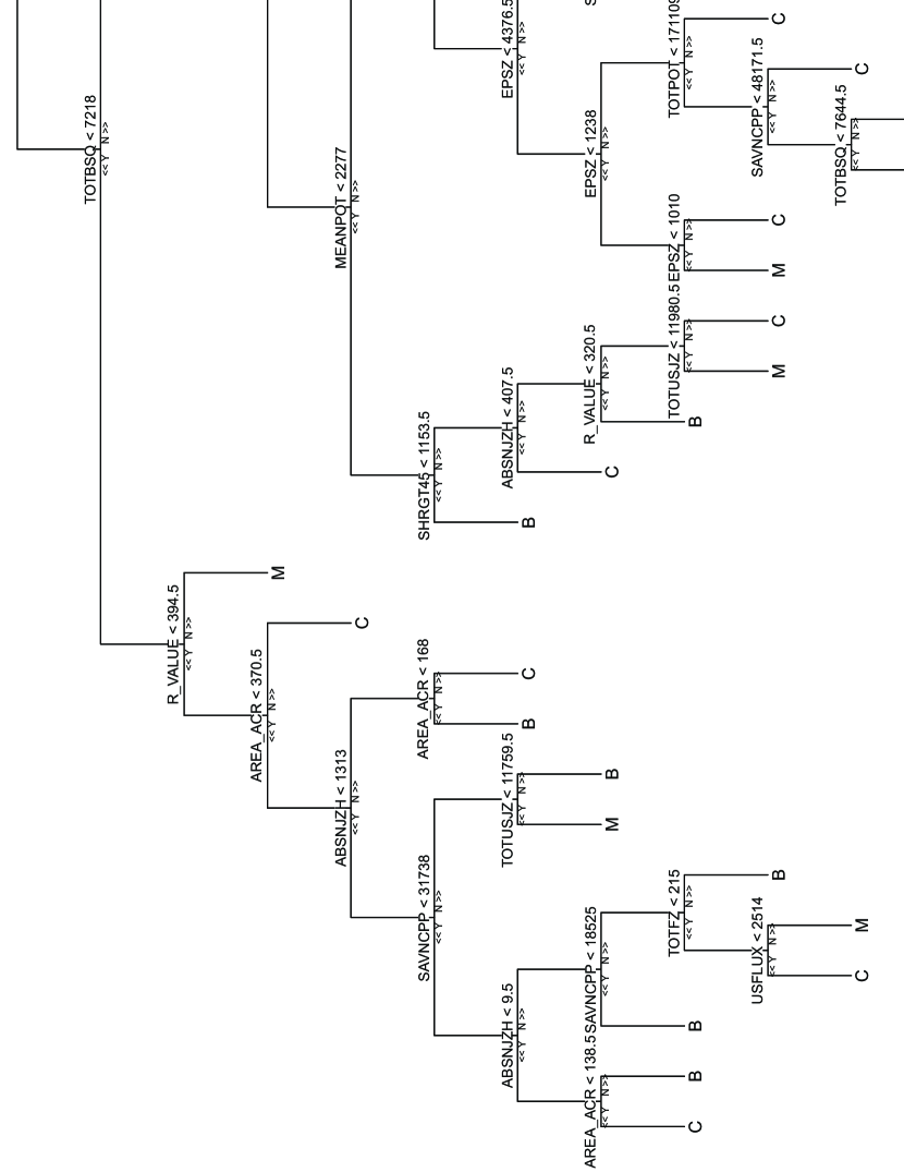
Figure 3: A sample representative tree grown by the RF algorithm.

References

- Abramenko (2005) Abramenko, V. I. 2005, ApJ, 629, 1141
- Ahmed et al. (2013) Ahmed, O. W., Qahwaji, R., Colak, T., et al. 2013, Sol. Phys., 283, 157
- Bailey et al. (2007) Bailey, S., Aragon, C., Romano, R., et al. 2007, ApJ, 665, 1246
- Barnes & Leka (2008) Barnes, G., & Leka, K. D. 2008, ApJ, 688, L107
- Barnes et al. (2007) Barnes, G., Leka, K. D., Schumer, E. A., & Della-Rose, D. J. 2007, Space Weather, 5, S09002
- Barnes et al. (2016) Barnes, G., Leka, K. D., Schrijver, C. J., et al. 2016, ApJ, 829, 89
- Bloomfield et al. (2012) Bloomfield, D. S., Higgins, P. A., McAteer, R. T. J., & Gallagher, P. T. 2012, ApJ, 747, L41
- Bobra & Couvidat (2015) Bobra, M. G., & Couvidat, S. 2015, ApJ, 798, 135
- Bobra et al. (2014) Bobra, M. G., Sun, X., Hoeksema, J. T., et al. 2014, Sol. Phys., 289, 3549
- Breiman (2001) Breiman, L. 2001, Machine Learning, 45, 5
- Breiman et al. (1984) Breiman, L., Friedman, J. H., Olshen, R. A., & Stone, C. J. 1984, Classification and Regression Trees (Monterey, CA: Wadsworth and Brooks)
- Breiman et al. (2003) Breiman, L., Last, M., & Rice, J. 2003, Random Forests: Finding Quasars (New York, NY: Springer New York), 243–254
- Carliles et al. (2010) Carliles, S., Budavári, T., Heinis, S., Priebe, C., & Szalay, A. S. 2010, ApJ, 712, 511
- Daglis et al. (2004) Daglis, I., Baker, D., Kappenman, J., Panasyuk, M., & Daly, E. 2004, Space Weather, 2, S02004
- Dasgupta (2014) Dasgupta, A. 2014, reprtree: Representative trees from ensembles, r package version 0.6
- Denig et al. (2012) Denig, W., Green, J., Rodriguez, J., & Viereck, R. 2012, in COSPAR Meeting, Vol. 39, 39th COSPAR Scientific Assembly, 442
- Farrell et al. (2015) Farrell, S. A., Murphy, T., & Lo, K. K. 2015, ApJ, 813, 28
- Fisher et al. (2012) Fisher, G. H., Bercik, D. J., Welsch, B. T., & Hudson, H. S. 2012, Sol. Phys., 277, 59
- Gallagher et al. (2002) Gallagher, P. T., Moon, Y.-J., & Wang, H. 2002, Sol. Phys., 209, 171
- Geurts et al. (2006) Geurts, P., Ernst, D., & Wehenkel, L. 2006, Mach. Learn, 63, 3
- Guyon & Elisseeff (2003) Guyon, I., & Elisseeff, A. 2003, J. Mach. Learn. Res., 3, 1157
- Hanssen & Kuipers (1965) Hanssen, A. W., & Kuipers, W. J. A. 1965, Meded, Verh., 81, 2
- Hodge (2014) Hodge, K. A. 2014, PhD thesis, California Institute of Technology
- James et al. (2013) James, G., Witten, D., Hastie, T., & Tibshirani, R. 2013, An Introduction to Statistical Learning: With Applications in R (Springer Publishing Company, Incorporated)
- Japkowicz & Stephen (2002) Japkowicz, N., & Stephen, S. 2002, Intell. Data Anal., 6, 429
- Kuhn (2008) Kuhn, M. 2008, Journal of Statistical Software, 28, 1
- Laing et al. (2012) Laing, C., Wen, D., Wang, J. T. L., & Schlick, T. 2012, Nucleic Acids Research, 40, 487
- Leka & Barnes (2003) Leka, K. D., & Barnes, G. 2003, ApJ, 595, 1296
- Leka & Barnes (2007) —. 2007, ApJ, 656, 1173
- Liaw & Wiener (2002) Liaw, A., & Wiener, M. 2002, R News, 2, 18
- Liu et al. (2010) Liu, C., Liu, R., Xu, Y., & Wang, H. 2010, in BAAS, Vol. 41, 403.10
- Meyer et al. (2017) Meyer, D., Dimitriadou, E., Hornik, K., Weingessel, A., & Leisch, F. 2017, e1071: Misc Functions of the Department of Statistics, Probability Theory Group (Formerly: E1071), TU Wien, r package version 1.6-8
- Nishizuka et al. (2017) Nishizuka, N., Sugiura, K., Kubo, Y., et al. 2017, ApJ, 835, 156
- Pesnell et al. (2012) Pesnell, W. D., Thompson, B. J., & Chamberlin, P. C. 2012, Sol. Phys., 275, 3
- Priest & Forbes (2002) Priest, E. R., & Forbes, T. G. 2002, A&A Rev., 10, 313
- R Core Team (2016) R Core Team. 2016, R: A Language and Environment for Statistical Computing, R Foundation for Statistical Computing, Vienna, Austria
- Schou et al. (2012) Schou, J., Scherrer, P. H., Bush, R. I., et al. 2012, Sol. Phys., 275, 229
- Schrijver (2007) Schrijver, C. J. 2007, ApJ, 655, L117
- Song et al. (2009) Song, H., Tan, C., Jing, J., et al. 2009, Sol. Phys., 254, 101
- Sun et al. (2014) Sun, X., et al. 2014, ArXiv e-prints 1405.7353, arXiv:1405.7353
- Wang & Liu (2015) Wang, H., & Liu, C. 2015, RAA, 15, 145
- Welsch et al. (2009) Welsch, B. T., Li, Y., Schuck, P. W., & Fisher, G. H. 2009, ApJ, 705, 821
- Woodcock (1976) Woodcock, F. 1976, Monthly Weather Review, 104, 1209
- Yuan et al. (2010) Yuan, Y., Shih, F. Y., Jing, J., & Wang, H.-M. 2010, RAA, 10, 785
- Zhao & Cen (2013) Zhao, Y., & Cen, Y., eds. 2013, Data Mining Applications with R, ISBN 978-0124115118 (Academic Press, Elsevier)