Group galaxy number density profiles far out: is the ‘one-halo’ term NFW out to $>10$ virial radii?

Abstract

While the density profiles (DPs) of $\Lambda$CDM haloes obey the NFW law out to roughly one virial radius, $r_{\rm vir}$, the structure of their outer parts is still poorly understood, because the 1-halo term describing the halo itself is dominated by the 2-halo term representing the other halos picked up. Using a semi-analytical model, we measure the real-space 1-halo number DP of groups out to 20 $r_{\rm vir}$ by assigning each galaxy to its nearest group above mass $M_{\rm a}$, in units of the group $r_{\rm vir}$. If $M_{\rm a}$ is small (large), the outer DP of groups falls rapidly (slowly). We find that there is an optimal $M_{\rm a}$ for which the stacked DP resembles the NFW model to 0.1 dex accuracy out to 13 virial radii. We find similar long-range NFW surface DPs (out to 10 $r_{\rm vir}$) in the SDSS observations using a galaxy assignment scheme that combines the non-linear virialized regions of groups with their linear outer parts. The optimal $M_{\rm a}$ scales as the minimum mass of the groups that are stacked to a power 0.25–0.3. The NFW model thus does not solely originate from violent relaxation. Moreover, populating haloes with galaxies using HOD models must proceed out to much larger radii than usually done.

1 Introduction

Cosmological dissipationless N-body simulations have taught us that, regardless of their mass, the radial density profiles (DPs) of haloes in the range of $\approx$ 0.01 to 1.5 virial radii ($r_{\rm vir}$) are well described by the Navarro, Frenk & White (1996, NFW) model whose inner and outer slopes are respectively $-1$ and $-3$ (Navarro et al. 2004 find that the Einasto 1969 model provides an even better representation of the DP, with a more progressive change of slopes).

The origin of the NFW profile could be a combination of fast and slow accretion in the inner and outer region, respectively (e.g., Lu et al. 2006), where the fast accretion is generally related to violent relaxation. The total DP is understood to be the sum of two terms (as first introduced by Cooray & Sheth 2002 in the context of galaxy clustering): the 1-halo term describing the halo itself, and the 2-halo term describing the other haloes around the first one, following the 2-point correlation function of haloes. Beyond a few $r_{\rm vir}$, the 1- and 2-halo terms respectively correspond to an extension of the halo and the other haloes outside. While several authors studied the sum of both terms beyond $r_{\rm vir}$ (e.g., Prada et al.; Hayashi & White 2008; Diemer & Kravtsov 2014), they all assumed possibly truncated NFW or Einasto profiles for the 1-halo term (and their stacked DPs involved multiple counting). Hence, the 1-halo term is poorly known beyond $\approx\,2\,r_{\rm vir}$.

In this Letter, we assign galaxies in a semi-analytical model (SAM) of galaxy formation to their nearest group in units of the group’s $r_{\rm vir}$. This allows us to explore the 1-halo term by measuring the DPs of groups traced by their galaxies out to $20\,r_{\rm vir}$. We then compare these DPs to the galaxy surface number density profiles (SDPs) of groups in the Sloan Digital Sky Survey (SDSS), also out to $20\,r_{\rm vir}$, using a novel scheme to assign each galaxy to its closest group in redshift space. In Sect. 2, we describe the simulation and data used. Our assignment scheme is explained in Sect. 3 and in Sect. 4 we present the results of our study. Finally, we summarize and discuss our results in Sect. 5. Masses and distances are given in physical units, and we adopt the $\Lambda$CDM cosmology with $\Omega_{\rm m}=0.275$, $\Omega_{\Lambda}=0.725$, and ${H_{0}=70.2~{}\hbox{km s}^{-1}\hbox{Mpc}^{-1}}$ (WMAP7, Komatsu et al., 2011).

2 Observations and simulation

2.1 SDSS galaxies and groups

The observational sample of galaxies was retrieved from the SDSS-DR12 (Alam et al., 2015) database. We selected all galaxies from the Main Galaxy Sample that are in the redshift range $0.01\leq z\leq 0.05$ and are more luminous than $\mathcal{M}^{\rm Petro}_{r}\leq-18.78$, where $\mathcal{M}_{r}^{\rm Petro}$ corresponds to the k-corrected absolute Petrosian magnitude in the $r$-band. These criteria lead to a doubly-complete subsample in distance and luminosity containing $63,642$ galaxies. The k-corrections were computed with the kcorrect code (version 4_2) of Blanton & Roweis (2007), and we obtained the magnitude limit of the sample using a geometric approach similar to that of Garilli, Maccagni & Andreon (1999).

The galaxy groups were selected from the updated version of the catalogue compiled by Yang et al. (2007). The new catalogue contains 473,482 groups drawn from a sample of 601,751 galaxies mostly from the Sloan Digital Sky Survey’s Data Release 7 (SDSS-DR7, Abazajian et al., 2009).

The radii $r_{200,{\rm m}}$ (of spheres that are 200 times denser than the mean density of the Universe) are derived from the $M_{200,{\rm m}}$ masses given in the Yang et al. catalogue, which are based on abundance matching with the group luminosities. We then determined the virial radii, $r_{\rm vir}$, the corresponding virial masses, $M_{\rm vir}=(\Delta_{\rm v}/2)\,H^{2}(z)\,r_{\rm vir}^{3}/G$, and virial velocities $v_{\rm vir}=\sqrt{\Delta_{\rm v}/2}\,H(z)\,r_{\rm vir}$, defined such that the mean densities within the virial sphere are $\Delta_{\rm v}$=100 times the critical density of the Universe, by assuming the NFW DP and the concentration-mass relation of Dutton & Macciò (2014).

To avoid incomplete profiles of SDSS groups, we first assure that at least $95\%$ of the region within ${20\,r_{\rm vir}}$ from the group centres lies within the SDSS coverage area. For this purpose, we adopted the SDSS-DR7 spectroscopic angular selection function mask provided by the NYU Value-Added Galaxy Catalog team (Blanton et al., 2005) and assembled with the package Mangle 2.1 (Hamilton & Tegmark, 2004; Swanson et al., 2008). We also require that the groups lie far enough from the redshift limits of the galaxy sample ($z_{\rm min}=0.01$ and $z_{\rm max}=0.05$), by only selecting groups within the redshift range $[{z_{\rm min}+20\,\Delta z,z_{\rm max}-20\,\Delta z}]$, where ${\Delta z={\sqrt{{2}/{\Delta_{\rm v}}}\,(1+z_{\rm group})}\,v_{\rm vir}/c}$, where $c$ is the speed of light (see Sect. 3). These criteria lead to a sample of $1961$ groups with $\log(M_{\rm vir}/{\rm M_{\odot}})$ $\geq 12.5$.

2.2 Simulations

We used the SAM by Henriques et al. (2015), which was run on the Millennium-II simulations (Boylan-Kolchin et al., 2009). We extracted the snapshot corresponding to $z=0$ from the Henriques2015a..MRIIscPlanck1 table in the Virgo–Millennium database of the German Astrophysical Virtual Observatory (GAVO).

From the simulation box extracted from GAVO, we built a mock flux-limited, SDSS-like sample of groups and galaxies. Since the simulation box is not large enough to produce the SDSS-like group catalogue, we replicated the simulation box along the three Cartesian coordinates, then placed an observer at some position and mapped the galaxies on the sky. The absolute magnitudes in the $r$-band (including internal dust extinction) were converted to apparent magnitudes, and the flux limit of the Main Galaxy Sample of the SDSS, ${m_{r}<17.77}$, was applied.

We then select the galaxies and groups from the mock catalogue following the same selection criteria that is applied to the observations and presented in Sect. 2.1. In particular, the doubly complete mock subsample, again limited to luminosities $\mathcal{M}^{\rm Petro}_{r}\leq-18.78$, contains 61,915 galaxies. We apply the SDSS spectroscopic mask to the mock data.

3 Membership assignment scheme

To assign galaxies to the group that attracts them the most, one requires selecting the group with the lowest distance to the group in units of virial radius, $d$ (since acceleration decreases with distance in all models with density slopes steeper than –1 everywhere). This is straightforward in our real-space (3D) sample. In our redshift-space (2+1D) sample, for galaxies far away from the group, we estimate $d$ using the standard redshift-space distance

$$d_{\rm outer}(R,\Delta z)=\sqrt{\frac{\Delta_{\rm v}}{2}\left[\frac{c\,\Delta z}{v_{\rm vir}(1+z_{\rm group})}\right]^{2}+\left(\frac{R}{r_{\rm vir}}\right)^{2}}\ .$$ (1)

For a galaxy lying close to a group, we take into account the strong redshift distortions by applying the overdensity in projected phase space (PPS), $P_{M}(R,\Delta z)$ introduced by Yang et al. (2005, 2007), which is the suitably scaled product of the NFW SDP times a Gaussian distribution of galaxy-group redshift differences. We convert this overdensity to an equivalent redshift-space distance by joining the two estimators at a fixed number of virial radii, $\widetilde{R}_{\rm n}$, marking the transition from the non-linear group to the linear outer regions. This amounts to

$$d_{\rm inner}(R,\Delta z)=\left(\frac{a-\ln P_{M}(R,\Delta z)}{b}\right)^{1/2},$$ (2)

where $b=1/(\eta^{2}\,\Delta_{\rm v})$ while $a$ is given by

$$a=\frac{\widetilde{R}_{n}^{2}}{\eta^{2}\,\Delta_{\rm v}}+\ln\left(\frac{2}{3}\,\sqrt{\frac{\Delta_{\rm v}}{\pi}}\,\frac{H(z)}{H_{0}}\frac{c_{\rm v}^{2}\,g(c_{\rm v})}{\Omega_{\rm M}\,\eta\,(1+z)}f(\widetilde{R}_{n})\right)\ .$$ (3)

In eq. (3), $c_{\rm v}$ is the concentration parameter, ${1/g(c_{\rm v})=\ln(1+c_{\rm v})-c_{\rm v}/(1+c_{\rm v})}$, and

$$f(\widetilde{R})={2\pi\,\Sigma(R)\,r_{\rm vir}^{2}\over c_{\rm v}^{2}\,g\!\left(c_{\rm v}\right)\,N_{\rm vir}}=\frac{1-|c_{\rm v}^{2}\tilde{R}^{2}-1|^{-1/2}\ C^{-1}[1/(c_{\rm v}\tilde{R})]}{c_{\rm v}^{2}\tilde{R}^{2}-1}\ ,$$

where $C^{-1}(x)=\cos^{-1}x$ or $\cosh^{-1}x$, depending on whether $x<1$ or $x>1$. Analyzing the galaxy assignments from the 3D SAM projected into the PPS, we deduce that $\widetilde{R}_{\rm n}=2.5$. A more detailed description of our approach, as well as the full derivation of eqs. (2) and (3) are given in a forthcoming paper (Trevisan et al. 2017, in prep.)

3.1 Group mass thresholds for the assignment

We consider two group mass thresholds. The first one, $M_{\rm s}$, corresponds to the minimum virial mass of the groups in our sample around which we are measuring the number DPs. The second, $M_{\rm a}$, is the lowest group mass to which we can assign galaxies.. When $M_{\rm a}$ is extremely low, most galaxies outside the virial radius of a group are assigned to their one-galaxy groups, leaving few galaxies beyond that radius. On the other hand, if $M_{\rm a}$ is large, we partially pick up the 2-halo term in our group DP.

4 Results

4.1 Three-dimensional number density profiles

Fig. 1 shows the galaxy number DPs obtained in the simulations for stacked groups from the SAM with $\log(M_{\rm vir}/{\rm M_{\odot}})$ $>13.0$, using 3 different values of $M_{\rm a}$. We fit the parameters of the NFW and Einasto models using maximum likelihood estimation (MLE); therefore, no binning of the data is required. The MLE was performed considering only the galaxies within the region $0.1\leq r/r_{\rm vir}\leq 2$.

The middle and bottom panels in Fig. 1 shows the residuals of the best-fit profiles. For $\log(M_{\rm a}/{\rm M}_{\odot})=12.3$, the NFW describes the density profile very well to 0.1 dex accuracy out to $r\sim 13~{}r_{\rm vir}$. On the other hand, the Einasto form fails to describe the DP in the outer regions, as shown in the bottom panel in Fig. 1. A reasonable fit requires including the outer regions in the MLE procedure. For that model, fitting the profile between $0.1\leq r/r_{\rm vir}\leq 8$ leads to 0.1 dex residuals from $r\sim 0.2$ $r_{\rm vir}$ to $\sim 13\,r_{\rm vir}$, with best-fit parameters $c_{\rm v}=5.5\pm 0.8$ and $n=8.9\pm 0.6$.

4.2 Surface density profiles and comparison with observations

Applying the method described in Sect. 3 to the SDSS data, we obtain the SDP shown in Fig. 2. Since our scheme is designed to assign galaxies within a sphere of radius 20 $r_{\rm vir}$, we compare the SDP with that of the NFW model computed by integrating the 3D DP along the line-of-sight within that sphere (its analytical form is provided in appendix B.1 of Mamon, Biviano & Murante 2010).

In Fig. 2, the observed profile is also compared to the projection of the 3D profile shown in Fig. 1. The excellent agreement between the profile of SDSS groups and the simulation can be clearly seen, and the difference between the the best-fit $c_{\rm v}$ values are within the errors. This indicates that our scheme for distances in redshift-space for the SDSS sample is a good approximation to the 3D space assignment.

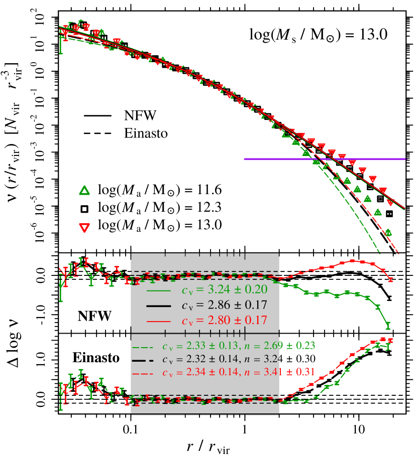
Figure 1: Number density profile of 525 stacked groups with $\log(M_{\rm s}/\rm M_{\odot})=13.0$ from the simulation. Galaxies were assigned to groups of minimum mass as indicated. The mass threshold ${\log(M_{\rm a}/{\rm M}_{\odot})=12.3}$ (black) leads to the density profile that is best described by the NFW model out to ${r\sim 13~{}r_{\rm vir}}$ (see Sect. 4.3), with residuals of $\pm 0.1$ dex (middle panel). The purple horizontal line represent the mean density of the Universe. The middle and bottom panels show the residuals of the best-fit NFW and Einasto profiles. The shaded areas indicate the region considered in the fitting procedure ($0.1<r/r_{\rm vir}<2$), and the long and short-dashed horizontal lines respectively indicate $\Delta\log\nu=0$ and $\pm 0.1$ dex. The colours are the same as in the upper panel, and the best-fit parameters are indicated in each panel. The errors in the data points are from 1000 bootstraps on the groups combined with Poisson, while those on parameters $c_{\rm v}$ and $n$ are from those bootstraps.

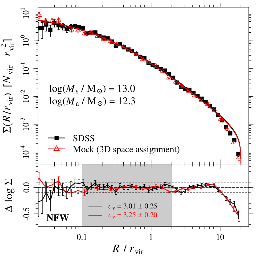
Figure 2: Surface number density profiles of stacked groups from the simulations (red, 525 groups) and SDSS data (black, 534 groups). The upper panel shows the stacked profile of groups with $\log(M_{\rm vir}/{\rm M_{\odot}})$ $\geq 13.0$ obtained for ${\log(M_{\rm a}/{\rm M}_{\odot})=12.3}$. The profile from the simulations is the projection of the profile shown in Fig. 1. The residuals of the best-fit NFW profiles limited to the $20$ $r_{\rm vir}$ sphere are shown in the bottom panel, where the shaded area indicates the region where the fit is performed (${0.1<R/r_{\rm vir}<2}$). The long and short-dashed horizontal lines indicate $\Delta\log\Sigma=0$ and $\pm 0.1$ dex, respectively. The colours are the same as in the upper panel, and the concentration parameters $c_{\rm v}$ of the best fits are presented. The error bars are as in Fig. 1.

4.3 Group mass thresholds

In Sects. 4.1 and 4.2, we showed that the NFW profile is a good description of both the simulation and the SDSS data for groups more massive than $\log(M_{\rm s}/{\rm M}_{\odot})$ $=13$ when $\log(M_{\rm a}/{\rm M}_{\odot})$ $=12.3$. However, does this result still hold for different values of $M_{\rm s}$ and $M_{\rm a}$?

To tackle this question, we considered different group samples with $M_{\rm vir}\geq M_{\rm s}$ with $\log(M_{\rm s}/{\rm M}_{\odot})$ ranging from $12.5$ to $14$, in steps of $0.1$ dex. For each of these samples, we fit the NFW profile in the region from $0.1$ to $2$ $r_{\rm vir}$, and, from the extrapolation of the best fit, we compute the predicted number of galaxies within the region from $2$ to $10$ $r_{\rm vir}$, $N^{\rm NFW}_{\rm outer}$. We then determine the the best value of $M_{\rm a}$ for each $M_{\rm s}$, which corresponds to the one leading to $\Delta N=N^{\rm NFW}_{\rm outer}-N^{\rm obs}_{\rm outer}=0$, where $N^{\rm obs}_{\rm outer}$ is the observed number of galaxies within the region $2$ to $10$ $r_{\rm vir}$.

The resulting values of $M_{\rm a}$ that provide the closest match to the NFW model up to very large radii (hereafter, $M_{\rm a}^{\rm NFW}$) are shown as a function of $M_{\rm s}$ in Fig. 3. For $\log(M_{\rm s}/{\rm M}_{\odot})$ ranging from $12.5$ to $14$, the values of $\log(M_{\rm a}^{\rm NFW}/\rm M_{\odot})$ vary from $\sim$12.2 to $\sim$12.8. We fitted $M_{\rm a}^{\rm NFW}$ as a function of $M_{\rm s}$ with a linear relation ${\log M_{\rm a}^{\rm NFW}=\alpha+\beta\log M_{\rm s}}$, finding

$$\!\!\!\!\begin{array}[]{l}\alpha=9.52\pm 0.16\,,\ \beta=0.21\pm 0.01\ ({\rm SDSS}),\\ \alpha=9.24\pm 0.18\,,\ \beta=0.24\pm 0.01\ ({\rm mock\ in\ projection}),\\ \alpha=8.04\pm 0.22\,,\ \beta=0.33\pm 0.02\ ({\rm mock\ in\ 3D\ space}).\\ \end{array}\!\!$$

For $\log(M_{\rm s}/{\rm M}_{\odot})$ $\mathrel{\hbox{\hbox to0.0pt{\hbox{\lower 4.0pt\hbox{$\sim$}}\hss}\hbox{$>$}}}13.0$, the values of $M_{\rm a}^{\rm NFW}$ for the 3D profiles are slightly higher than those for the projected profiles, because we minimise $\Delta N$ within $r=2$ to $10$ $r_{\rm vir}$, which does not exactly correspond to the same range in projection.

The residuals of the best fits of $\log(M_{\rm a}/{\rm M}_{\odot})$ for the cases when $\log(M_{\rm s}/{\rm M}_{\odot})$ $=12.5$, $13.0$, $13.5$, and $14.0$ are presented in Fig. 4. In all cases, the DP is matched to within 0.1 dex by the NFW model out to $\sim 12$ to $14$ $r_{\rm vir}$ in real space and $10\,r_{\rm vir}$ in projection.

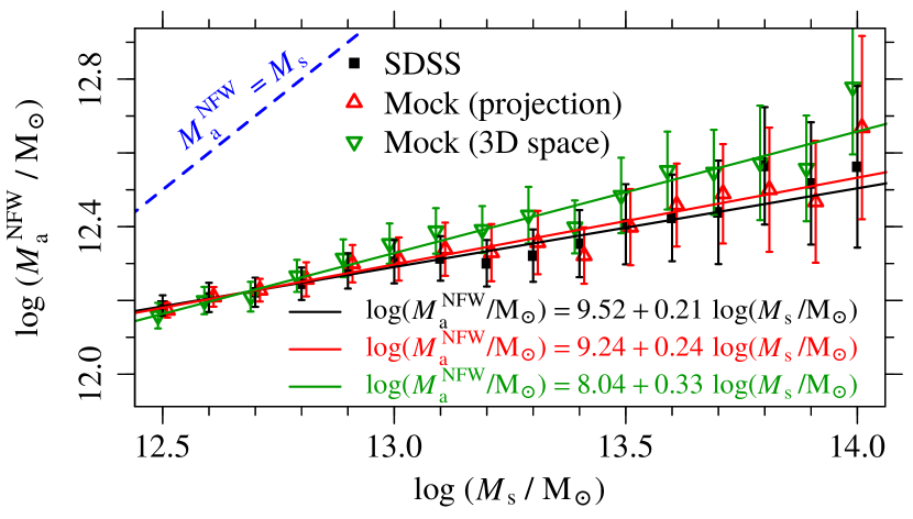
Figure 3: Best-fit group mass threshold $M_{\rm a}^{\rm NFW}$ to obtain NFW density profiles out to $10\,r_{\rm vir}$ versus the minimum sample group mass $M_{\rm s}$. The plot shows the results from the SDSS data (black symbols), the simulations in 3D (green), and in projection (red). The errors in $M_{\rm a}^{\rm NFW}$ were estimated by bootstrapping the groups of each sample $200$ times, and the best linear fits to the $\log M_{\rm a}^{\rm NFW}$ versus $\log M_{\rm s}$ relation are shown as solid lines, while $M_{\rm a}^{\rm NFW}=M_{\rm s}$ is shown as a dashed blue line.

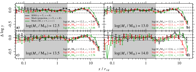
Figure 4: Residuals of the density profiles relative to the best NFW fit, for four values of $M_{\rm s}$. The curves correspond to the results for the SDSS data (black lines), the simulations in projection (red) and in 3D (green). For the 3D number density profile, $\Delta\equiv\Delta\nu$ and $x\equiv r$, the 3D radial distance to the group centre. For the projected profiles (black and red lines), $\Delta\equiv\Delta\Sigma$ and $x\equiv R$, the projected distance to the group centre. The shaded areas indicate the region of the fitting procedure ($0.1<x/r_{\rm vir}<2$). The values of $M_{\rm a}$ correspond to the optimal values shown in Fig. 3. The error bars are as in Fig. 1.

5 Conclusions and Discussion

In this Letter, we investigated the 1-halo term of the galaxy number DPs of groups and clusters out to $20$ virial radii, analyzing both a recent state-of-the-art semi-analytical model of galaxy formation based on the Millennium-II simulations, as well as a complete sample of galaxies in and around groups and clusters from SDSS-DR7. We assigned galaxies to the nearest group in units of that group’s virial radius, which is straightforward in 3D. In 2+1D, we use a scheme to estimate 3D distances by combining the non-linear behaviour within $2.5\,r_{\rm vir}$ and redshift space distances beyond. Our assignment method involves two group mass thresholds: the minimum group mass in our sample, $M_{\rm s}$, and the minimum group mass, $M_{\rm a}$, to which we assign galaxies.

Our main findings can be summarized as follows:

• For $\log(M_{\rm a}/{\rm M}_{\odot})$ $=12.3$, the NFW formula describes very well the density profile of $\log(M_{\rm vir}/{\rm M_{\odot}})$ $\geq 13.0$ groups out to far beyond the virial radius, for both the simulations (Fig. 1) and observations (Fig. 2). Our best NFW fit, performed in the range 0.1 to $2\,r_{\rm vir}$ (where the NFW model is known to fit the galaxy distribution, Carlberg et al. 1997), has residuals of 0.1 dex out to distances as large as ${r\sim 13~{}r_{\rm vir}}$ (where the density is one-tenth of the mean density of the Universe) and projected distances $R\sim 10\,r_{\rm vir}$. Our best-fit concentrations for SDSS ($c_{\rm v}=3.0$) are close to the mean of the values (corrected to our definition of $r_{\rm vir}$) of $c_{\rm v}=5.1$ (Carlberg et al., 1997), $c_{\rm v}=4.0$ (Lin et al., 2004), and $c_{\rm v}=2.6$ (Collister & Lahav, 2005).

• On the other hand, the Einasto formula fails to describe the density profile if the best-fit parameters are estimated using only galaxies in the inner regions ($0.1<R/r_{\rm vir}<2$, Fig. 1). A good fit is obtained only when the outer regions are included in the fitting procedure.

• For all values of $\log(M_{\rm s}/{\rm M}_{\odot})$ between 12.5 and 14, i.e., from small groups to clusters of galaxies, we are always able to find a value of $M_{\rm a}=M_{\rm a}^{\rm NFW}$ (Fig. 4), ranging from $\sim 10^{12.2}$ to $10^{12.8}~{}{\rm M}_{\odot}$ (with $\log M_{\rm a}$ varying linearly with $\log M_{\rm s}$, Fig. 3), that leads to profiles that are very well described by the NFW law out to $\mathrel{\hbox{\hbox to0.0pt{\hbox{\lower 4.0pt\hbox{$\sim$}}\hss}\hbox{$>$}}}10\,r_{\rm vir}$ (even if the Einasto law can also lead to good fits).

When $M_{\rm a}$ is large, our measurement of the density profile is increasingly contaminated by the 2-halo term at increasingly large distances (it appears concave in log-log). When $M_{\rm a}$ is very low, most of the galaxies beyond a few virial radii are assigned to very low mass, often single-galaxy, haloes, leaving a truncated density profile (convex in log-log). There is, therefore, an intermediate value of $M_{\rm a}$ that represents the transition between these two regimes.

However, it was not obvious that intermediate values of $M_{\rm a}$ would lead to density profiles (both in 3D and in projection) that 1) are consistent with the $-3$ outer slope of the NFW model as far out as 10 virial radii and 2) are the extrapolation of the NFW model fit only up to $2\,r_{\rm vir}$. This suggests that one could re-define the 1-halo term as that for which the outer density profile of singly-assigned objects (galaxies in groups) follows an NFW model.

It is intriguing that the DPs of groups appear NFW-like out to $10\,r_{\rm vir}$ for the appropriate choice of $M_{\rm a}$. Admittedly, the origin of the power-law relation between the optimal $M_{\rm a}$ and $M_{\rm s}$ remains to be clarified. Nevertheless, if this NFW behaviour at large distances for optimal values of $M_{\rm a}$ is not fortuitous, the origin of the outer part of the NFW model would be more complex than previously thought. Beyond $4\,r_{\rm vir}$, a galaxy is expanding away from its nearest group, but is decelerated by this group. So, the outer $-3$ slope of the NFW model may have to do with the combination of the primordial density field with the spherical collapse model instead of halo mergers or slow accretion.

We observe ‘V’-shape kinks in the mock 1-halo DPs and SDPs at $\simeq 2.2\,r_{\rm vir}$ and at $\simeq 2.8\,r_{\rm vir}$ in the SDSS 1-halo SDPs (Fig. 4), similar to those discovered in the total DPs (Diemer & Kravtsov, 2014) and total SDSS SDP (More et al., 2016). The presence of these kinks in our 1-halo DPs and SDPs indicates that these are natural features of the 1-halo term related to the 2nd apocentre of orbits (backsplash radius).

Many teams have been creating virtual galaxy catalogues by populating galaxies in haloes using Halo Occupation Distribution models, and nearly all truncate their galaxy distributions at $r\simeq r_{\rm vir}$. Our results indicate that one should instead populate haloes with galaxies out to $\simeq 13\,r_{\rm vir}$ of until one reaches the next nearest group.

If the primordial density field drives the density profiles of groups at such large distances, one may wonder whether it also is responsible for the variation of galaxy properties such as the increasing fraction of star forming galaxies up to $\approx 8\,r_{\rm vir}$ observed by von der Linden et al. (2010). We investigate this question in Trevisan et al. (2017, in prep.).

References

- Abazajian et al. (2009) Abazajian K. N., et al., 2009, ApJS, 182, 543
- Alam et al. (2015) Alam S., et al., 2015, ApJS, 219, 12
- Blanton & Roweis (2007) Blanton M. R., Roweis S., 2007, AJ, 133, 734
- Blanton et al. (2005) Blanton M. R., et al., 2005, AJ, 129, 2562
- Boylan-Kolchin et al. (2009) Boylan-Kolchin M., Springel V., White S. D. M., Jenkins A., Lemson G., 2009, MNRAS, 398, 1150
- Carlberg et al. (1997) Carlberg R. G., et al., 1997, ApJL, 485, L13
- Collister & Lahav (2005) Collister A. A., Lahav O., 2005, MNRAS, 361, 415
- Cooray & Sheth (2002) Cooray A., Sheth R., 2002, Physics Reports, 372, 1
- Diemer & Kravtsov (2014) Diemer B., Kravtsov A. V., 2014, ApJ, 789, 1
- Dutton & Macciò (2014) Dutton A. A., Macciò A. V., 2014, MNRAS, 441, 3359
- Einasto (1969) Einasto J., 1969, Astrophysics, 5, 67
- Garilli et al. (1999) Garilli B., Maccagni D., Andreon S., 1999, A&A, 342, 408
- Hamilton & Tegmark (2004) Hamilton A. J. S., Tegmark M., 2004, MNRAS, 349, 115
- Hayashi & White (2008) Hayashi E., White S. D. M., 2008, MNRAS, 388, 2
- Henriques et al. (2015) Henriques B. M. B., White S. D. M., Thomas P. A., Angulo R., Guo Q., Lemson G., Springel V., Overzier R., 2015, MNRAS, 451, 2663
- Komatsu et al. (2011) Komatsu E., et al., 2011, ApJS, 192, 18
- Lin et al. (2004) Lin Y.-T., Mohr J. J., Stanford S. A., 2004, ApJ, 610, 745
- Lu et al. (2006) Lu Y., Mo H. J., Katz N., Weinberg M. D., 2006, MNRAS, 368, 1931
- Mamon et al. (2010) Mamon G. A., Biviano A., Murante G., 2010, A&A, 520, A30
- More et al. ( 2016) More S., et al., 2016, ApJ, 825, 39
- Navarro et al. (1996) Navarro J. F., Frenk C. S., White S. D. M., 1996, ApJ, 462, 563
- Navarro et al. (2004) Navarro J. F., et al., 2004, MNRAS, 349, 1039
- Prada et al. (2006) Prada F., Klypin A. A., Simonneau E., Betancort-Rijo J., Patiri S., Gottlöber S., Sanchez-Conde M. A., 2006, ApJ, 645, 1001
- Swanson et al. (2008) Swanson M. E. C., Tegmark M., Hamilton A. J. S., Hill J. C., 2008, MNRAS, 387, 1391
- Trevisan et al. (2017) Trevisan M., Mamon G. A., Khosroshahi H. G., 2017, MNRAS, 464, 4593
- Yang et al. (2005) Yang X., Mo H. J., van den Bosch F. C., Weinmann S. M., Li C., Jing Y. P., 2005, MNRAS, 362, 711
- Yang et al. (2007) Yang X., Mo H. J., van den Bosch F. C., Pasquali A., Li C., Barden M., 2007, ApJ, 671, 153
- von der Linden et al. (2010) von der Linden A., Wild V., Kauffmann G., White S. D. M., Weinmann S., 2010, MNRAS, 404, 1231