Modelling the unfolding pathway of biomolecules: theoretical approach and experimental prospect

Abstract

We analyse the unfolding pathway of biomolecules comprising several independent modules in pulling experiments. In a recently proposed model, a critical velocity $v_{c}$ has been predicted, such that for pulling speeds $v>v_{c}$ it is the module at the pulled end that opens first, whereas for $v<v_{c}$ it is the weakest. Here, we introduce a variant of the model that is closer to the experimental setup, and discuss the robustness of the emergence of the critical velocity and of its dependence on the model parameters. We also propose a possible experiment to test the theoretical predictions of the model, which seems feasible with state-of-art molecular engineering techniques.

1 Introduction

The development of the so-called single-molecule experiments in the last decades has made it possible to carry out research at the molecular level. Biophysics is, undoubtedly, one of the fields where these techniques have had a bigger impact, triggering a whole new area of investigation on the elastic properties of biomolecules. Recent accounts of the current development of this enticing field can be found in Refs. R06 ; KyL10 ; MyD12 ; HyD12 .

Atomic force microscopy (AFM) stands out because of its extensive use. In particular, the role played by AFM in the study of modular proteins is crucial COFMBCyF99 ; FMyF00 ; HDyT06 . Figure 1 shows a sketch of the experimental setup in a pulling experiment of a molecule comprising several modules. The biomolecule is stretched between the platform and the tip of the cantilever. The spring constant of the cantilever is $k_{c}$, which is usually in the range of $100$ pN/nm. Here, we consider the simplest situation, in which the total length of the system $\Delta Z_{p}=\Delta Z_{c}+X$ is controlled. The stretching of the molecule makes the cantilever bend by $\Delta Z_{c}$, and then the force can be recorded as $F=k_{c}\Delta Z_{c}$.

The outcome of the above described experiment is a force-extension curve, similar to panel b) in Fig. 1. This force-extension curve provides a fingerprint of the elastomechanical properties of the molecule under study. When molecules composed of several structural units, such as modular polyproteins, are pulled, a sawtooth pattern comes about in the force-extension curve COFMBCyF99 ; FMyF00 ; HDyT06 . At certain values of the length, there are almost vertical “force rips”: each force rip marks the unfolding of one module. Interestingly, these force rips already appear when the molecule is quasi-statically pulled, a limit that can be explained by means of an equilibrium statistical mechanics description PCyB13 . When the molecule is pulled at a finite rate, the appearance of these force rips can still be explained by the system partially sweeping the metastable region of the equilibrium branches BCyP15 .

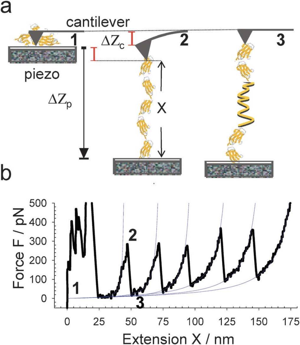
Figure 1: a: Sketch of the experimental setup in an AFM experiment with a modular protein. The position of the platform is shifted $\Delta Z_{p}$ from 1 to 2, producing an elongation of $X$ over the molecule and bending the cantilever a magnitude $\Delta Z_{c}$. From 2 to 3 the force is almost relaxed because of the unravelling of one of the modules. b: Force-extension curve in a typical lenght-control AFM experiment with a polyprotein. Each rip in the force accounts for the unfolding of a module. Taken from MyD12 .

The unfolding pathway is, roughly, the order and the way in which the structural units of the system unravel. It has been recently found out that the unfolding pathway depends on the pulling velocity and the pulling direction HDyT06 ; LyK09 ; GMTCyC14 ; KHLyK13 . Particularly, in GMTCyC14 , different unfolding pathways are observed in SMD simulations on the Maltose Binding Protein. The authors reported that for low pulling speeds the first unit to unfold is the least stable, whereas for high pulling speed it is the closest to the pulled end, regardless of their relative stability.

Very recently, a toy-like model has been proposed to qualitatively understand the above experimental framework PCCyP15 . Specifically, each module is represented by a nonlinear spring, characterised by a bistable free energy that depends on the module extension. Therein, the two basins represent its folded and unfolded states. The spatial structure of the system is retained in its simplest way: each module extends from the end point of the previous one to its own endpoint (which coincides with the start point of the next). Moreover, each module endpoint obeys an overdamped Langevin equation with forces stemming from the bistable free energies and white noise forces with amplitudes verifying the fluctuation-dissipation theorem.

In the above model, the unfolding pathway was found to depend on the pulling velocity. In the simplest non-trivial case, there is only one module that is different from the rest, which is also the furthest from the pulled end. In this situation, only one critical velocity $v_{c}$ shows up: for pulling velocities $v_{p}>v_{c}$, it is the weakest module that opens first but for $v_{p}>v_{c}$ it is the module at the pulled end. In addition, analytical results were derived for this critical velocity by introducing some approximations: mainly two, (i) perfect length control and (ii) the deterministic approximation, that is, our neglecting of the stochastic forces. This was done by means of a perturbative solution of the deterministic equations in both the pulling velocity and an asymmetry parameter, which measures how different the potentials of the modules are.

The main aim of this work is twofold. First, we would like to refine the above theoretical framework, making it closer to the experimental setup in AFM. In particular, we would like to look into the effect of a more realistic modelling of the length-control device. Instead of considering perfect length-control, we consider a device with a finite value of the stiffness, both at the end of the one-dimensional chain (as originally depicted in Ref. PCCyP15 ) and at the start point thereof, which is where it is usually situated in the AFM experiments, see Fig. 1. Second, we would like to discuss how our theory could be checked in a real experiment with modular proteins.

This chapter is structured as follows. First, we introduce the original model and discuss its most relevant results in section 2. In section 3, we study the role played by the location of the restoring spring and the finite value of its spring constant. We provide some details about the free energy modelling employed for each of the modules in section 4. Section 5 is devoted to discuss a possible AFM experiment in order to test our theory. Finally, we wrap up the main conclusions which emerge from our work.

2 Revision of the model and previous results

Here, we briefly review the model that was originally put forward in Ref. PCCyP15 . We consider a polyprotein comprising $N$ modules. When the molecule is stretched, the simplest description is to portray it as a one-dimensional chain. We define the coordinates $q_{i},$ $(i=0,\ldots,N)$ in such a way that the $i$-th unit extends from $q_{i-1}$ to $q_{i}$, the extension of the $i$-th unit is $x_{i}=q_{i}-q_{i-1}$. Moreover, as shown in Fig. 2, the pulling device is assumed to be connected to the right (pulled) end of the chain.

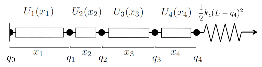
Figure 2: Sketch of the model for a molecule comprising four units. Therein, the units are denoted by rectangles and have potentials $U_{i}(x_{i})$, with $x_{i}$ being the extension of the $i$-th unit’s. The unit endpoints $q_{i}$ are represented by the beads, and the extensions are thus $x_{i}=q_{i}-q_{i-1}$ (by definition, $q_{0}=0$). The spring stands for the length-controlling device attached to the pulled end $q_{4}$, whose contribution to the system free energy is assumed to be harmonic with stiffness $k_{c}$.

We assume Langevin dynamics for the $q_{i}$ coordinates ($q_{0}=0$),

$$\gamma\dot{q}_{i}=-\frac{\partial}{\partial q_{i}}A(q_{0},\ldots,q_{N})+\zeta_{i}\qquad i>0,$$ (1)

in which the $\zeta_{i}$ are Gaussian white noise forces, such that

$$\langle\zeta_{i}(t)\rangle=0,\qquad\langle\zeta_{i}(t)\zeta_{j}(t^{\prime})\rangle=2\gamma k_{B}T\delta_{ij}\delta(t-t^{\prime}),$$ (2)

with $k_{B}$ being the Boltzmann constant, and $\gamma$ and $T$ being the friction coefficient (assumed to be common for all the units) and the temperature of the fluid in which the protein is immersed, respectively. The global free energy function of the system is

$$A(q_{0},\ldots,q_{N})=\sum_{i=1}^{N}U_{i}(q_{i}-q_{i-1})+\frac{1}{2}k_{c}(L-q_{N})^{2}.$$ (3)

In the previous equation, we have considered an elastic term due to the finite stiffness $k_{c}$ of the controlling device, which is located at the pulling end as shown in Fig. 2. Finally, $L$ stands for the desired length program and $U_{i}(x_{i})$ is the single unit contribution, which only depends on the extension, to $A$. Consequently, the force exerted over the biomolecule is $k_{c}(L-q_{N})$. We consider length-controlled experiments at constant pulling velocity, that is, $\dot{L}=v_{p}$.

When $k_{c}\to\infty$, the control over the length is perfect and $q_{N}\to L$ in such a way that $k_{c}(L-q_{N})\to F$, being $F$ a Lagrange multiplier. That is, the perfect length-controlled situation is the same that a force-controlled one but with $F$ the force needed to maintain a total length equal to $L$. Note that there is no contribution to the free energy coming from the pulling device in this limit, since $k_{c}(L-q_{N})^{2}/2=F^{2}/(2k_{c})\to 0$.

The approach in Ref. PCCyP15 tries to keep things as simple as possible. Then, the evolution equations for the extensions are written by assuming (i) perfect length control and (ii) the deterministic approximation, obtained by neglecting the noise terms. Note that the evolution equations in the latter approximation are sometimes called the macroscopic equations vK92 , which are

$$\gamma\dot{x}_{1} =-U^{\prime}_{1}(x_{1})+U^{\prime}_{2}(x_{2}),$$ (4a)

$$\gamma\dot{x}_{i} =-2U^{\prime}_{i}(x_{i})+U^{\prime}_{i+1}(x_{i+1})+U^{\prime}_{i-1}(x_{i-1}),\quad 1<i<N,$$ (4b)

$$\gamma\dot{x}_{N} =-2U^{\prime}_{N}(x_{N})+U^{\prime}_{N-1}(x_{N-1})+F,$$ (4c)

$$F =\gamma v_{p}+U^{\prime}_{N}(x_{N}).$$ (4d)

So far, nothing has been said about the shape of the single-unit contributions $U_{i}$ to the free energy. In order to maintain a general approach, we only request the functions $U_{i}(x)-Fx$ to become a double well for some interval of forces. Each well stands for the folded and the unfolded basins of each module. Now, we separate these functions in a main part common to all units and a separation from this main part weighted by an asymmetry parameter $\xi$,

$$U_{i}(x)=U(x)+\xi\delta U_{i}(x),\quad U^{\prime}_{i}(x)=U^{\prime}(x)+\xi\delta f_{i}(x).$$ (5)

We have done the same separation in the derivative, by defining $\delta f_{i}(x)=\delta U^{\prime}_{i}(x)$.

It is possible to solve the system (4) by means of a perturbative expansion in the pulling velocity $v_{p}$ and the asymmetry $\xi$. Indeed, if we retain only linear order terms in $v_{p}$ and $\xi$, the corrections due to finite pulling rate and asymmetry are not coupled. This perturbative solution, when the system starts from an initial condition in which all the units are folded, is shown to be PCCyP15

$$x_{i}=\ell+\frac{\xi\overline{\delta f}-v_{p}\gamma\dfrac{N^{2}-1}{6N}}{U^{\prime\prime}(\ell)}+\frac{v_{p}\gamma\dfrac{i(i-1)}{2N}-\xi\delta f_{i}(\ell)}{U^{\prime\prime}(\ell)},$$ (6)

where $\ell=L/N$ stands for the specific length per module and the over-bar means average over the units. Note that, if all the free energies are equal ($\xi=0$) and we are not pulling ($v_{p}=0$), the total length will be reasonably equally distributed among all the units. Moreover, it is worth emphasising that this solution is approximate, it diverges when $U^{\prime\prime}(\ell)\to 0$. This shows that this perturbative solution breaks down when the average length per module $\ell$ reaches the stability threshold $\ell_{b}$, such that $U^{\prime\prime}(\ell_{b})=0$.

We are interested in a criterion that allows us to discern which unit is the first to unfold and we hope that our perturbative solution is good enough in this regard. Since the folded state ceases to exist when $x$ reaches $\ell_{b}$, it is reasonable to assume that the first module to unfold is precisely the one for which $x_{i}=\ell_{b}$ is attained for the shortest time. In Eq. (6), we can see that the finite pulling term favours the unfolding of modules that are nearer to the pulled end, whereas the asymmetry term favours the unfolding of the weaker units (those with the lowest values of $\delta f_{i}$).

We can compute the pulling velocities $v^{i}(j)$ for which each couple of modules $(i,j)$, $j>i$, reach simultaneously the stability threshold. They are determined by the condition

$$x_{i}(\ell_{c})=x_{j}(\ell_{c})=\ell_{b},$$ (7)

which gives both the value of $\ell_{c}$ (or time $t_{c}$) at which the stability threshold is reached and the relationship between $v_{p}$ and $\xi$. Then, in a specific system with known $\delta f_{i}$’s we can predict what are the critical velocities that separate regions inside which the first unit to unfold is different. In Ref. PCCyP15 , some examples of the use of this theory are provided, which show a good agreement with simulations of the Langevin dynamics (1).

The simplest configuration in which a critical velocity arises is the following. Let us consider a chain of $N$ units, all of them with the same contribution to the free energy, except the first one (the furthest to the pulled end). Therefore, $\delta f_{i}(x)=0$, $i\neq 1$, $\delta f_{1}(x)\neq 0$. Moreover we will assume that $\delta f_{1}(\ell_{b})<0$, that is, the first module is weaker than the rest. For such a configuration, there appears only one critical velocity, which is given by PCCyP15

$$\frac{\gamma v_{c}}{\xi}=-\frac{\delta f_{1}(\ell_{b})}{N-1}.$$ (8)

For $v_{p}<v_{c}$, the first module to unfold is the weakest one, whereas for $v_{p}>v_{c}$ the unfolding starts from the pulled end. In Ref. PCCyP15 , a more general situation is investigated but, here, we restrict ourselves to this configuration.

3 Relevance of the stiffness

In a real AFM experiment, the stiffness is finite and, as a result, the control over the length is not perfect. Furthermore, the position that is externally controlled is, usually, that of the platform and the main elastic force stems from the bending of the tip of the cantilever, as depicted in Fig. 1. Thus, it seems more reasonable to model the pulling of the biomolecule in the way sketched in Fig. 3.

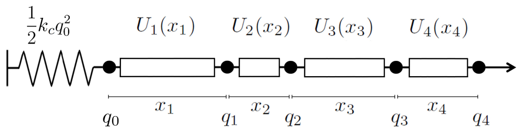
Figure 3: Sketch of the model for a protein with four units. It is identical toFig. 2, except for the position of the length-controlling device, which is now located at the fixed end.

Some authors HyS03 have used other elastic reactions that reflect the attachment by means of flexible linkers among the platform and the pulled end $q_{N}$, and between consecutive modules. Here, we will consider a perfect absorption, in order to keep the model as simple as possible. In the next two subsections, we study the effect of the finite value of the stiffness $k_{c}$ and the location of the spring, respectively, on the unfolding pathway.

3.1 Finite stiffness

Here, we still consider the model depicted in Fig. 2, that is, the spring is situated at the end of the chain, but with a finite value of the stiffness $k_{c}$. Also, we consider the macroscopic equations (zero noise), which are

$$\gamma\dot{x}_{1} =-U^{\prime}_{1}(x_{1})+U^{\prime}_{2}(x_{2}),$$ (9a)

$$\gamma\dot{x}_{i} =-2U^{\prime}_{i}(x_{i})+U^{\prime}_{i+1}(x_{i+1})+U^{\prime}_{i-1}(x_{i-1}),\quad 1<i<N,$$ (9b)

$$\gamma\dot{x}_{N} =-2U^{\prime}_{N}(x_{N})+U^{\prime}_{N-1}(x_{N-1})+k_{c}\left(L-\sum_{k=1}^{N}x_{k}\right).$$ (9c)

This system differs from that in Eq. (4) because in the last equation the Lagrange multiplier $F$ is substituted by the harmonic force $k_{c}(L-\sum_{k=1}^{N}x_{k})$. As in the previous case, this system is analytically solvable by means of a perturbative expansion in $v_{p}$ and $\xi$. The approximate solution for the extension $x_{i}$ is

$$x_{i}=\ell + \frac{\xi Nk_{c}\overline{\delta f}(\ell)-v_{p}\gamma k_{c}\dfrac{[3U^{\prime\prime}(\ell)+k_{c}(N-1)]N(N+1)}{6[Nk_{c}+U^{\prime\prime}(\ell)]}}{U^{\prime\prime}(\ell)[Nk_{c}+U^{\prime\prime}(\ell)]}$$ (10)

$$+ \frac{v_{p}\gamma k_{c}i(i-1)-2\xi[Nk_{c}+U^{\prime\prime}(\ell)]\delta f_{i}(\ell)}{2U^{\prime\prime}(\ell)[Nk_{c}+U^{\prime\prime}(\ell)]}.$$

Here $\ell\neq L/N$, it stems from the relation

$$U^{\prime}(\ell)=k_{c}(L-N\ell).$$ (11)

We can see easily how we reobtain (6) taking the limit $k_{c}\to\infty$ in (10), as it should be. Although the solution is slightly different, it still breaks down when $U^{\prime\prime}(\ell)$ vanishes, that is, when $\ell\to\ell_{b}$. Therefore, to the lowest order, again we have to seek a solution of (7), with the extensions given by (10), and substitute $\ell_{c}\simeq\ell_{b}$ therein. This leads to the same critical velocities found for the infinite stiffness limit.

3.2 Location of the elastic reaction

As depicted in Fig. 1, in an AFM experiment the distance between the moving platform and the fixed cantilever is the controlled quantity. Then, the model sketched in Fig. 3 is closer to the experimental setup: the left end corresponds to the fixed cantilever, with $q_{0}$ standing for $\Delta Z_{c}$, and the right end represents the moving platform. Thus, the free energy of this setup is given by

$$A(q_{0},\ldots,q_{N})=\sum_{i=1}^{N}U_{i}(q_{i}-q_{i-1})+\frac{1}{2}k_{c}q_{0}^{2}\,.$$ (12)

From the free energy (12), we derive the Langevin equations by making use of Eq. (1). The macroscopic equations (zero noise) read

$$\gamma\dot{x}_{1} =-2U^{\prime}_{1}(x_{1})+U^{\prime}_{2}(x_{2})+k_{c}\left(L-\sum_{k=1}^{N}x_{k}\right),$$ (13a)

$$\gamma\dot{x}_{i} =-2U^{\prime}_{i}(x_{i})+U^{\prime}_{i+1}(x_{i+1})+U^{\prime}_{i-1}(x_{i-1}),\quad 1<i<N,$$ (13b)

$$\gamma\dot{x}_{N} =-U^{\prime}_{N}(x_{N})+U^{\prime}_{N-1}(x_{N-1})+v_{p}.$$ (13c)

In the infinite stiffness limit, $k_{c}\to\infty$, the harmonic contribution tends to a new Lagrange multiplier $F$ such that $\sum x_{i}=L$. Therefrom, it is obtained that $F=U_{1}^{\prime}(x_{1})$ and the resulting system is exactly equal to that in Eq. (4). This is logical: if the spring is totally stiff and then the control over the length is perfect, the two models are identical.

The system (13) can be solved in an analogous way, by means of a perturbative expansion in the asymmetry $\xi$ and the pulling velocity $v_{p}$. The result is

$$x_{i}=\ell + \frac{\xi Nk_{c}\overline{\delta f}(\ell)-v_{p}\gamma k_{c}\dfrac{[3U^{\prime\prime}(\ell)+k_{c}(N-1)]N(N+1)}{6[Nk_{c}+U^{\prime\prime}(\ell)]}}{U^{\prime\prime}(\ell)[Nk_{c}+U^{\prime\prime}(\ell)]}$$ (14)

$$+ \frac{v_{p}\gamma k_{c}i\left(i-1+\dfrac{2U^{\prime\prime}(\ell)}{k_{c}}\right)-2\xi[Nk_{c}+U^{\prime\prime}(\ell)]\delta f_{i}(\ell)}{2U^{\prime\prime}(\ell)[Nk_{c}+U^{\prime\prime}(\ell)]}.$$

Again, we can reobtain (6) taking the infinite stiffness limit in (14). Although the final solution for the extension is different from the previous one, when we look for the critical velocities and make the approximation $\ell_{c}\simeq\ell_{b}$ we get the same analytical results for them.

Our main conclusion is that the existence of a set of critical velocities, setting apart regions where the first unit to unfold is different, is not an artificial effect of the limit $k_{c}\to\infty$. Indeed, at the lowest order, all the versions of the studied model, independently of the value of the stiffness and the location of the spring, give the same critical velocities. This robustness is an appealing feature of the theory, and makes it reasonable to seek this phenomenology in real experiments.

4 Shape of the bistable potentials

Different shapes for the double-well potentials have been considered in the literature, mainly simple Landau-like quartic potentials to understand the basic mechanisms underlying the observed behaviours PCyB13 ; BCyP15 ; GMTCyC14 and more complex potentials when trying to obtain a more detailed, closer to quantitative, description of the experiments BCyP15 ; BGUKyF10 ; BHPSGByF12 ; BCyP14 . For the sake of concreteness, we restrict ourselves to the proposal made by Berkovich et al. BGUKyF10 ; BHPSGByF12 . Therein, the free energy of a module is represented by the sum of a Morse potential, which mimics the enthalpic minimum of the folded state, and a worm-like-chain (WLC) term MyS95 , which accounts for the entropic contribution to the elasticity of the unfolded state. Specifically, the free energy is written as

$$U(x)=U_{0}\left[\left(1-e^{-2b\frac{x-R_{c}}{R_{c}}}\right)^{2}-1\right]+\frac{k_{B}T}{4P}L_{c}\left(\frac{1}{1-\frac{x}{L_{c}}}-1-\frac{x}{L_{c}}+\frac{2x^{2}}{L_{c}^{2}}\right).$$ (15)

This shape has shown to be useful for some pulling experiments with actual proteins as titin I27 or ubiquitin BGUKyF10 ; BHPSGByF12 . Therein, each parameter has a physical interpretation. First, in the WLC part, we have: (i) the contour length $L_{c}$, which is the maximum length for a totally extended protein, and (ii) the persistence length $P$, which measures the characteristic length over which the chain is flexible. Both of them, $L_{c}$ and $P$, can be measured in terms of the number of amino acids in the chain. Second, for the Morse contribution, we have: (iii) $R_{c}$, which gives the location of the enthalpic minimum and (iv) $U_{0}$ and $b$, which measure the depth and the width (in a non-trivial form) of the folded basin. The stability threshold $\ell_{b}$ cannot be provided as an explicit function of the parameters in Berkovich et al.’s potential. However, we can always estimate it numerically, solving $U^{\prime\prime}(\ell_{b})=0$ for a specific set of parameters.

As we anticipated in section 2, here we will focus in a very specific configuration where only the first module is different from the rest. Consistently, we use $U(x)$ to represent the free energy of each of the identical modules, and $U_{1}(x)$ for that of the first one. In particular, we consider that the first unit has a slightly different contour length, $L_{c}+\Delta$. Therefore, we can linearise $U_{1}(x)$ around $U(x)$, using the natural asymmetry parameter $\xi=\Delta/L_{c}\ll 1$. Therefore,

$$U_{1}^{\prime}(x;L_{c}+\Delta)\simeq U^{\prime}(x;L_{c})+\xi\delta f_{1}(x;L_{c}),$$ (16)

where

$$\delta f_{1}(x;L_{c})\equiv L_{c}\frac{\partial U^{\prime}(x;L_{c})}{\partial L_{c}}=-\frac{k_{B}T}{2P}\left[\frac{\frac{x}{L_{c}}}{\left(1-\frac{x}{L_{c}}\right)^{3}}+\frac{2x}{L_{c}}\right].$$ (17)

This linearisation is useful for the direct application of our theory to some engineered systems, see the next section.

5 Experimental prospect

In the experiments, the observation of the unfolding pathway is not trivial at all. The typical outcome of AFM experiments is a force-extension curve (FEC) in which the identification of the unfolding events is, in principle, not possible when the modules are identical. Thus, in order to test our theory, molecular engineering techniques that manipulate proteins adding some extra structures, such as coiled-coil LSyM14 or Glycine SKSNyR03 probes, come in handy. For instance, a polyprotein in which all the modules except one have the same contour length may be constructed in this way. A reasonable model for this situation is a chain with modules described by Berkovich et al. potentials with the same parameters for all the modules, with the exception of the contour length of one of them. According to our theory, a critical velocity emerges (8) and it may be observed because the unfolding of the unit which is different can be easily identified in the FEC, see below.

Let us consider an example of a possible real experiment for a polyprotein with $N=10$ modules. We characterise the modules by Berkovich et al. potentials with parameters,

$$P=0.4\text{ nm}, L_{c}=30\text{ nm}, R_{c}=4\text{ nm},$$ (18a)

$$b=2, U_{0}=100\text{ pN}\,\text{ nm}, k_{B}T=4.2\text{ pN}\,\text{ nm},$$ (18b)

and the friction coefficient $\gamma=0.0028$pN nm^-1s BGUKyF10 . We call this system M₁₀: since all the modules are equal in M₁₀, it is not a very interesting system from the point of view of our theory. Nevertheless, we can consider a mutant species M${}^{\prime}_{10}$ that is identical to M₁₀ except for the module located in the first position (the fixed end), which has an insertion adding $\Delta$ to its contour length. Our theory gives an estimate for the critical velocity $v_{c}$ by using (8).

In Fig. 4, we compare the theoretical estimate for the critical velocity with the actual critical velocity obtained by integration of the dynamical system (13). Specifically, we have considered a system with spring constant $k_{c}=100$pN/nm. The numerical strategy to determine $v_{c}$ has been the following: starting from a completely folded state we let the system evolve obeying (13), with a “high” value of $v_{p}$ (well above the critical velocity), up to the first unfolding. We tune $v_{p}$ down until it is observed that the first module that unfolds is the weakest one: this marks the actual critical velocity. There are two theoretical lines: the solid line stems from the rigorous application of (8), with $\delta f_{1}$ given by (17), and $v_{c}$ is a linear function of $\xi$, whereas the dashed line corresponds to the substitution in (8) of $\xi\delta f_{1}(x)$ by $U_{1}^{\prime}(x;L_{c}+\Delta)-U^{\prime}(x;L_{c})$, without linearising in the asymmetry $\xi$. Note the good agreement between theory and numerics, specially in the “complete” theory where, for the range of plotted values, the relative error never exceeds 5$\%$. Interestingly, the computed values of the critical velocity lie in the range of typical AFM pulling speeds, from $10$ nm/s to $10^{4}$ nm/s AyA06 .

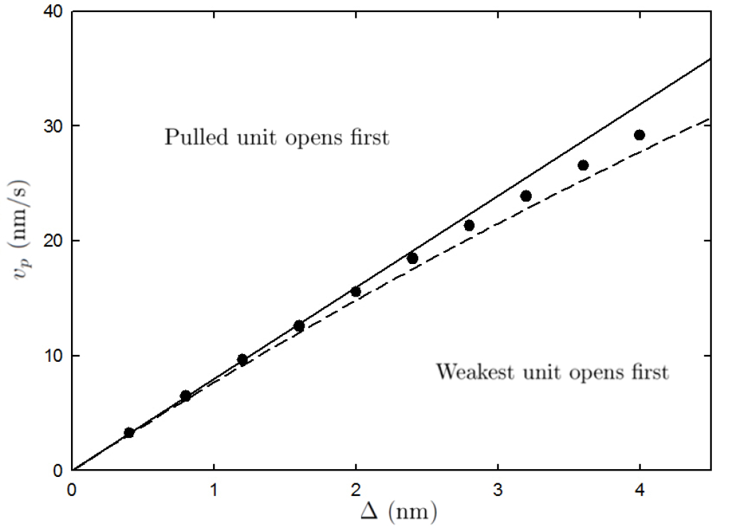
Figure 4: Critical velocities for M${}^{\prime}_{10}$ systems. The parameter $\Delta$ stands for the additional contour length of the first module. Numerical values (circles) are compared with two theoretical estimates: “complete” (dashed line) and linear (solid line).

Below $v_{c}$, it is always the weakest unit that unfolds first. Above $v_{c}$, the unit that unfolds first is the pulled one. For the sake of concreteness, from now we consider an specific molecule M${}^{\prime}_{10}$ fixing $\Delta=2$ nm. Using the linear estimation (17) in (8), we get a critical velocity $v_{c}\simeq 16$ nm/s that, as stated above, is in the range of the typical pulling speeds in AFM experiments.

In Fig. 5, we plot the extension of each unit vs the total extension $q_{N}-q_{0}$ in our notation ($X$ in Fig. 1), which is a good reaction coordinate ACDNKMNLyR10 . We have numerically integrated Eqs. (13) for two values of $v_{p}$: one below and one above $v_{c}$, namely $v_{p}=10$ nm/s and $v_{p}=22$ nm/s. The red trace stands for the weakest unit extension whereas the blue one corresponds to the pulled module. We can see that, for $v_{p}=10\text{ nm/s}<v_{c}$, the first unit that unfolds is the weakest one, whereas for $v_{p}=22\text{ nm/s}>v_{c}$ that is no longer the case. Specifically, the first unit that unfolds is the pulled one, and the weakest unfolds in the 4-th place.

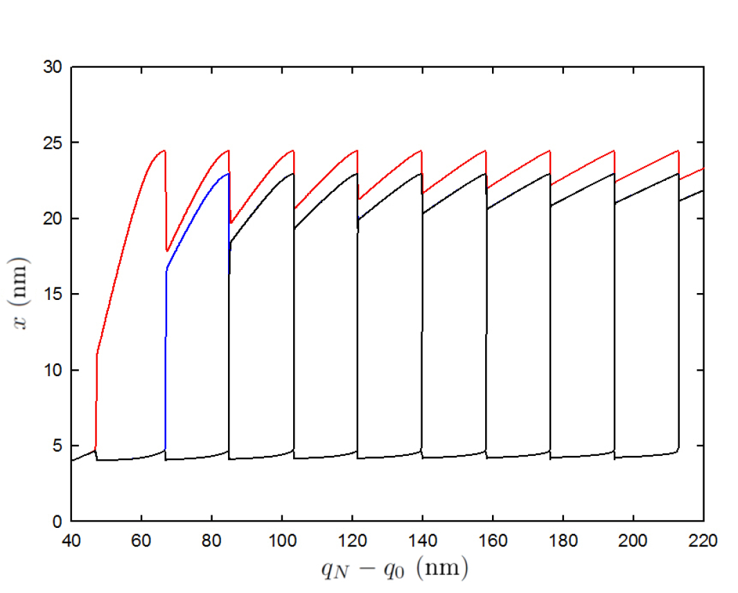
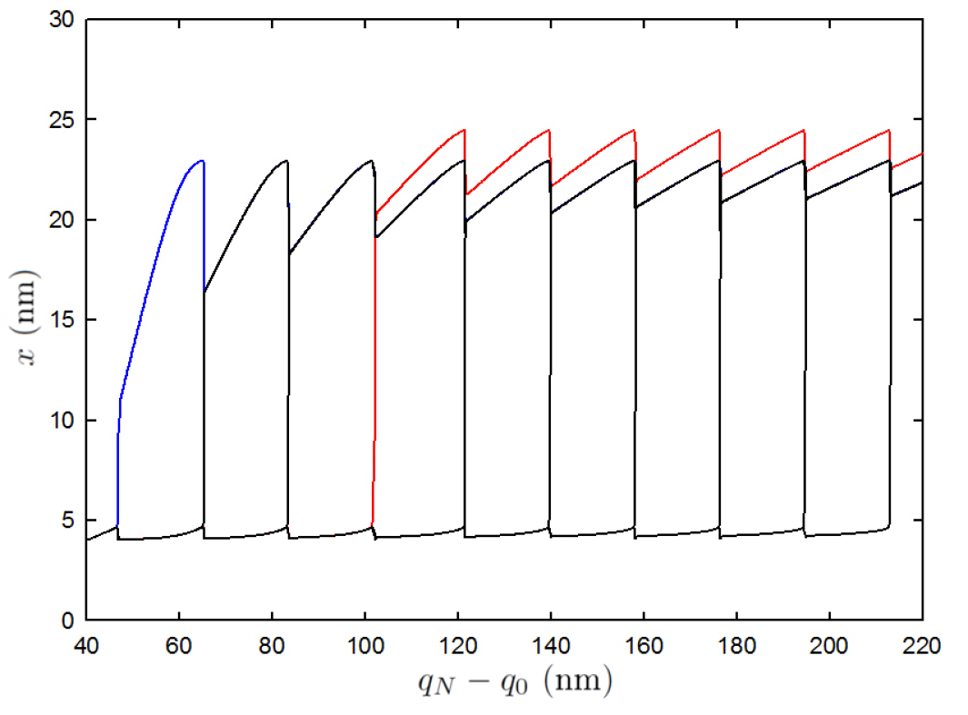
Figure 5: Evolution of the extensions of the different units as a function of the length of the system $q_{N}-q_{0}$ in a pulling experiment. The potential parameters are given in Eq. (18), and the pulling speeds are $v_{p}=10$ nm/s $<v_{c}$ (top) and $v_{p}=22$ nm/s $>v_{c}$ (bottom). The stiffness is $k_{c}=100$ pN/nm, which lies in the range of typical AFM values. The red line corresponds to the weakest unit and the blue line to the pulled one.

The plots in Fig. 5 are the most useful in order to detect the unfolding pathway of the polyprotein. Unfortunately, they are not accessible in the real experiments, for which the typical output is the FEC. Thus, we have also plotted the FEC in order to bring to light the expected outcome of a real experiment. In Fig. 6, we show the FEC for the two considered velocities in the same graph (solid line for the lower speed and dashed line for the higher one).

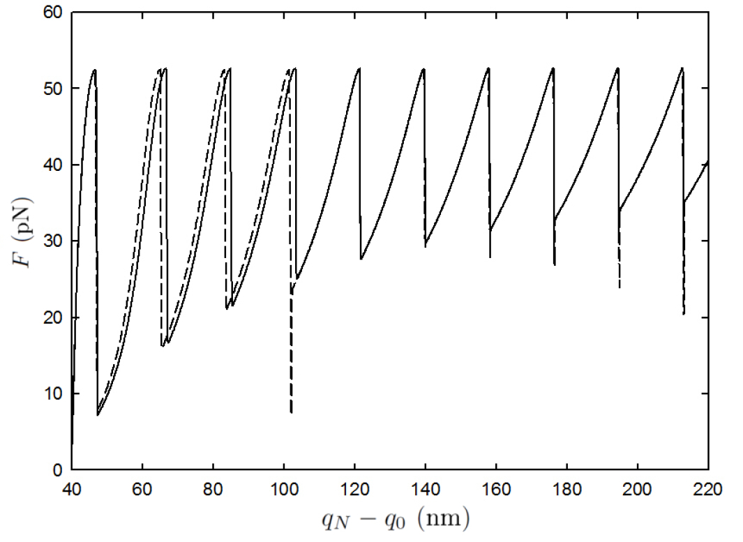
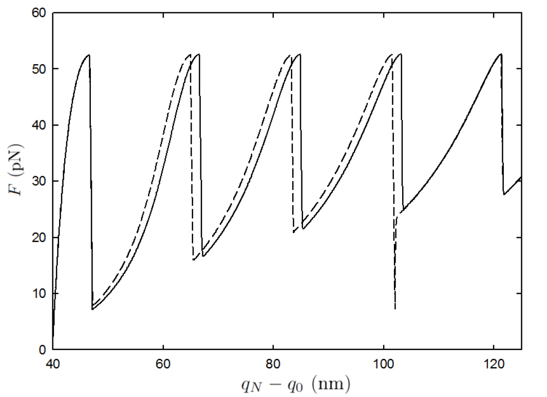
Figure 6: Top: FEC for the pulling experiment in Fig. 5. Two pulling speeds are considered, specifically $v_{p}=10$ nm/s (subcritical, solid) and $v_{p}=22$ nm/s (supercritical, dashed). Bottom: zoom of the region of interest, showing the shift between the peaks stemming from the increased contour length of the mutant module.

The FECS in Fig. 6 are superimposed until the first force rip, which corresponds to the first unfolding event (that of the mutant module for the slower velocity and that of the pulled unit for the faster one). As the mutant unit has a longer contour length than the rest, a shift between the curves in the next three pikes is found, because the effective contour length of the polyprotein has an extra contribution of $2$ nm. Reasonably, for the higher velocity, this shift disappears when the mutant module unfolds, and the curves are once again superimposed. This plot clearly shows how the existence of a critical velocity in a real experiment could be sought.

6 Conclusions

We have provided a useful theoretical framework in the context of modular proteins or, in general, of biomolecules comprising several units that unfold (almost) independently. Therein, according to our theory, it should be possible to find the emergence of a set of critical velocities which separate regions where the first module that unfolds is different. Although we focus on the biophysical application of the theory, it is worth highlighting that similar models are used in other fields. Many physical systems are also “modular”, since they comprise several units BZDyG16 , and thus a similar phenomenology may emerge. Some examples can be found in studies of plasticity MyV77 ; PyT02 , lithium-ion batteries DJGHMyG10 ; DGyH11 or ferromagnetic alloys BFSyG13 .

The development of our theory has shown that the position and value of the elastic constant $k_{c}$ of the length-controlled device is roughly irrelevant for the existence and value of the critical velocities. The derived expressions for the critical velocities are, to the lowest order, independent of the spring position and stiffness. Notwithstanding, our theory completely neglects the noise contributions and thus the units unfold when they reach their limit of stability, that is, at the force for which the folded basin disappears. This is expected to be relevant for biomolecules that follow the maximum hysteresis path, using the same terminology as in BZDyG16 ; BCyP15 , completely sweeping the metastable part of the intermediate branches of the FEC.

The numerical integration of the evolution equations for a realistic potential point out that our proposal for an experiment is, in principle, completely feasible. Therefore, our work encourages and motivates new experiments, in which the predicted features about the unfolding pathway of modular biomolecules could be observed. Finally, the discussion in the previous paragraph on the relevance of thermal noise makes it clear that an adequate choice of the biomolecule is a key point when trying to test our theory.

- (1) F. Ritort, J. Phys: Condens. Matter 18, R531 (2006)
- (2) D. Kumar, M. S. Li, Phys. Rep. 486, 1 (2010)
- (3) P. E. Marszalek, Y. F. Dufrêne, Chem. Soc. Rev. 41, 3523 (2012)
- (4) T. Hoffmann, L. Dougan, Chem. Soc. Rev. 41, 4781 (2012)
- (5) M. Carrión-Vázquez, A. F. Oberhauser, S. B. Fowler, P. E. Marszalek, S. E. Broedel, J. Clarke, J. M. Fernandez, Proc. Natl. Acad. Sci. USA 96, 3694 (1999)
- (6) T. E. Fisher, P. E. Marszalek, J. M. Fernandez, Nat. Struct. Biol. 7, 719 (2000)
- (7) C. Hyeon, R. I. Dima, D. Thirumalai, Structure 14, 1633 (2006)
- (8) A. Prados, A. Carpio, L. L. Bonilla, Phys. Rev. E 88, 012704 (2013)
- (9) L. L. Bonilla, A. Carpio, A. Prados, Phys. Rev. E 91, 052712 (2015)
- (10) M. S. Li, S. Kouza, J. Chem. Phys. 130, 145102 (2009)
- (11) C. Guardiani, D. Di Marino, A. Tramontano, M. Chinappi, F. Cecconi, J. Chem. Theory Comput. 10, 3589 (2014)
- (12) M. Kouza, C. K. Hu, M. S. Li, A. Kolinski, J. Chem. Phys. 139, 065103 (2013)
- (13) C. A. Plata, F. Cecconi, M. Chinappi, A. Prados, J. Stat. Mech. P08003 (2015)
- (14) N. G. van Kampen, Stochastic Processes in Physics and Chemistry (North-Holland, Amsterdam, 1992)
- (15) G. Hummer, A. Szabo, Biophys. J. 85, 5 (2003)
- (16) R. Berkovich, S. Garcia-Manyes, M. Urbakh, J. Klafter, J. M. Fernandez, Biophys. J. 98, 2692 (2010)
- (17) R. Berkovich, R. I. Hermans, I. Popa, G. Stirnemann, S. Garcia-Manyes, B. J. Bernes, J. M. Fernandez, Proc. Nat. Acad. Sci. 109, 14416 (2012)
- (18) L. L. Bonilla, A. Carpio, A. Prados, EPL 108, 28002 (2014)
- (19) J. F. Marko, E. D. Siggia, Macromolecules 28, 8759 (1995).
- (20) Q. Li, Z. N. Scholl, P. E. Marszalek, Angew. Chem. Int. Ed. 53, 13429 (2014)
- (21) I. Schwaiger, A. Kardinal, M. Schleicher, A. A. Noegel, M. Rief, Nat. Struct. Mol. Biol. 11, 81 (2003)
- (22) J. L. R. Arrondo, A. Alonso, Advanced Techniques in Biophysics (Springer, 2006)
- (23) G. Arad-Haase, S. G. Chuartzman, S. Dagan, R. Nevo, M. Kouza, B. K. Mai, H. T. Nguyen, M. S. Li, Z. Reich, Biophys. J. 99, 238 (2010)
- (24) I. Benichou, Y. Zhang, O. K. Dudko, S. Givli, J. Mech. Phys. Solids 95, 44 (2016)
- (25) I. M ller, P. Villaggio, Arch. Ration. Mech. Anal. 65, 25 (1977)
- (26) G. Puglisi, L. Truskinovsky, Contin. Mech. Thermodyn. 14, 437 (2002)
- (27) W. Dreyer, J. Jamnik, C. Guhlke, R. Huth, J. Moskon, M. Gaberscek, Nat. Mater. 9, 448 (2010)
- (28) W. Dreyer, C. Guhlke, M. Herrmann, Contin. Mech. Thermodyn. 23, 211 (2011)
- (29) I. Benichou, E. Faran, D. Shilo, S. Givli, Appl. Phys. Lett. 102, 011912 (2013)