Topology of irrationally indifferent attractors

Abstract.

We study the post-critical set of a class of holomorphic systems with an irrationally indifferent fixed point. We prove a trichotomy for the topology of the post-critical set based on the arithmetic of the rotation number at the fixed point. The only options are Jordan curves, a one-sided hairy Jordan curves, and Cantor bouquet. This explains the degeneration of the closed invariant curves inside the Siegel disks, as one varies the rotation number.

1. Introduction

1.1. Irrationally indifferent attractors

Let $f$ be a rational map of the Riemann sphere, or an entire function on the complex plane, with an irrationally indifferent fixed point at $0$. That is, near $0$,

$$f(z)=e^{2\pi i\alpha}z+O(z^{2})$$

for some $\alpha\in{\mathbb{R}}\setminus{\mathbb{Q}}$. The local dynamics of $f$ near $0$ depends on the arithmetic nature of $\alpha$ in a delicate fashion. By classical results of Siegel [Sie42] and Brjuno [Brj71], if $\alpha$ satisfies an arithmetic condition, now called Brjuno numbers, $f$ is conformally conjugate to the rotation by $2\pi\alpha$ on a neighbourhood of $0$. The maximal domain of linearisation (conjugacy) is called the Siegel disk of $f$ about $0$. When this happens, the local dynamics is rather trivial, any orbit starting near $0$ becomes dense in an invariant closed analytic curve. On the other hand, Yoccoz [Yoc88] showed that if $\alpha$ is not a Brjuno number, the quadratic polynomial

$$P_{\alpha}(z)=e^{2\pi i\alpha}z+z^{2}$$

is not linearisable at $0$. However, when the map is not linearisable near $0$, the local dynamics is not explained. In this paper, for the first time, we explain the delicate topological structure of the (local) attractor for some non linearisable maps.

The presence of an irrationally indifferent fixed point influences the global dynamics of the map. In a pioneering work on the iteration of holomorphic maps in 1910s, Fatou [Fat19] showed that there must be a critical point $c_{f}$ of $f$ which “interacts” with the fixed point $0$. Let $\Lambda(c_{f})$ denote the closure of the orbit of $c_{f}$, that is,

$$\Lambda(c_{f})=\overline{\cup_{i\geq 0}f^{\circ i}(c_{f})}.$$

Fatou showed that if $f$ is linearisable at $0$, the boundary of the Siegel disk at $0$ is contained in $\Lambda(c_{f})$, and if $f$ is not linearisable at $0$, $0\in\Lambda(c_{f})$. The set $\Lambda(c_{f})$ is part of the post-critical set of $f$, which is defined as the closure of the orbits of all critical points of $f$. By a general result in holomorphic dynamics, the post-critical set of $f$ is the measure theoretic attractor of the action of $f$ on its Julia set, [Lyu83]. For $P_{\alpha}$, $\Lambda(c_{P_{\alpha}})$ is the post-critical set, and hence it is the measure theoretic attractor of $P_{\alpha}$ on its Julia set. For arbitrary $f$, $\Lambda(c_{f})$ has its own basin of attraction in the Julia set of $f$, which a priori, may or may not have zero area.

The structure of $\Lambda(c_{f})$ for “badly approximable” rotation numbers $\alpha$ is well developed over the last four decades. For many classes of maps and rotation numbers, $c_{f}$ lies on the boundary of the Siegel disk, and $\Lambda(c_{f})$ is a Jordan curve, with some limitations on its geometry. These studies make use of the Siegel disk, through ingenious surgery procedures, which were introduced by Douady [Dou87] for quadratic polynomials, Zakeri [Zak99] for cubic polynomials, and Shishikura for all polynomials, in an unpublished work. Through these surgeries, the problem was linked to the dynamics of analytic circle homeomorphisms. Combining with the work of Yoccoz, Swianek and Herman [Yoc84, Swi98, Her79] on linearisation of analytic circle homeomorphisms, Douady concluded that if $\alpha$ is a rotation number of bounded type, $\Lambda(c_{P_{\alpha}})$ is a quasi-circle, equal to the boundary of the Siegel disk. The result of Douady was extended to cubic polynomials by Zakery [Zak99], to all polynomials by Shishikura, to all rational functions by Zhang [Zha11], and to a wide class of entire functions by Zakeri [Zak10]. On the other hand, in [McM98], McMullen successfully combined these ideas with renormalisation techniques, and among other results, concluded that when $\alpha$ is an algebraic number, $\Lambda(c_{f})$ enjoys rescaling self-similarity at $c_{p}$. In a far reaching generalisation, Petersen and Zakery [Pet96, PZ04] employed trans quasi-conformal surgery to prove that if the entries $a_{n}$ in the continued fraction of $\alpha$ satisfy $\log a_{n}=\mathcal{O}(\sqrt{n})$, $\Lambda(c_{P_{\alpha}})$ is a David circle (a Jordan curve with some control on its geometry). Moreover, they also show that under the same condition, the Julia set of $P_{\alpha}$ has $0$ area. This arithmetic condition holds for almost every $\alpha$. In light of these results, there is a satisfactory understanding of $\Lambda(c_{f})$ when there is some control on the growth of the entries in the continued fraction of $\alpha$. In contrast, at the other end of the spectrum, for rotation numbers with arbitrarily large entries, the structure of $\Lambda(c_{f})$ remained less developed. That is the main focus of this paper.

It is known that large entries in the continued fraction of $\alpha$ result in oscillations of the invariant curves in the Siegel disk. The size of an entry, and its location in the continued fraction, influences the shape of the oscillation. A large entry at the beginning of the continued fraction results in oscillations with large amplitude but small frequency, while the same large entry appearing later in the continued fraction results in oscillations with smaller amplitude but large frequency. See Fig 1. There are infinitely many entries in the continued fraction to play with. For an irrational number with many extremely large entries, the consecutive oscillations may build up and cause the degeneration of the closed invariant curves.

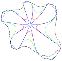
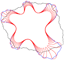
Figure 1. The figure on the left hand side shows the orbit of $c_{P_{\alpha}}$ for $\alpha=[2,2,\overline{2}]$, $[2,2,10^{2},\overline{2}]$, $[2,2,10^{4},\overline{2}]$, and $[2,2,10^{8},\overline{2}]$. The figure on the right hand side show the orbit of $c_{P_{\alpha}}$ for $\alpha=[2,2,\overline{2}]$, $[2,2,10^{2},\overline{2}]$, and $[2,2,10^{8},\overline{2}]$.

In 1997 Perez-Marco [PM97] showed that the closed invariant sets within Siegel disks do not disappear under perturbation of the rotation number. That is, for every $f$ with an irrationally indifferent fixed point at $0$, there is a non-trivial compact, connected, invariant set containing $0$, celled Siegel compacta or hedgehog. By successfully analysing these objects, he was able to build examples of non linearisable holomorphic germs with pathological behaviour, such as examples with no small cycles property [PM93], and examples with uncountably many conformal symmetries [PM95]. See [Bis08, Bis16, Che11] for more examples with unexpected features. But, these behaviours are not expected for rational functions, see for instance [ACE]. However, because those invariant sets are obtained through a limiting process, this approach provides limited control on those invariant sets for specific families of maps such as polynomials and rational functions. Also, the method does not apply near the boundary of the Siegel disks in order to study $\Lambda(c_{f})$.

Inou and Shishikura in 2006 [IS06] introduced a renormalisation scheme for the study of near parabolic maps. The scheme consists of an infinite dimensional class of maps ${\mathcal{F}}$, and a renormalisation operator which preserves ${\mathcal{F}}$. All maps in ${\mathcal{F}}$ have a certain covering structure on a region containing $0$, and in particular, have a (preferred) critical point. The set ${\mathcal{F}}$ contains some rational functions of arbitrarily large degrees. This scheme requires $\alpha$ to be of sufficiently high type, that is, $\alpha$ belongs to the set

$$\mathrm{HT}_{N}=\{\varepsilon_{0}/(a_{0}+\varepsilon_{1}/(a_{1}+\varepsilon_{2}/(a_{2}+\dots)))\mid\forall n\geq 0,a_{n}\geq N,\varepsilon_{n}=\pm 1\},$$

for a suitable $N$. This arithmetic class contains a Cantor set of rotation numbers; including some rotation numbers of bounded type, as well as some rotation numbers with arbitrarily large entries. Inou and Shishikura used this renormalisation scheme to trap the orbit of the critical point in a dynamically defined region about $0$. They showed that for every $f\in\mathcal{F}$, the orbit of $c_{f}$ is infinite, $\Lambda(c_{f})$ does not contain any periodic points, and in particular, $\Lambda(c_{f})$ is not equal to the Julia set of $f$. This renormalisation scheme was employed to prove the upper simi-continuity of $\Lambda(c_{f})$, at all bounded type rotation numbers in $\mathrm{HT}_{N}$ in [BC12] and all rotation numbers in $\mathrm{HT}_{N}$ in [Che19]. The former property was a main ingredient in the remarkable work of Buff and Cheritat [BC12] to build value of $\alpha$ such that the Julia set of $P_{\alpha}$ has positive area. These examples include both Brjuno and non Brjuno values of $\alpha$. In light of these developments, we understand that the unbounded regime of rotation numbers exhibit non trivial dynamics.

1.2. Statements of the results

In this paper we improve the control on $\Lambda(c_{f})$, and explain its delicate topological structure.

Theorem A (Trilogy of the post-critical set).

There is $N\geq 2$ such that for every $\alpha\in\mathrm{HT}_{N}$ and every $f(z)=e^{2\pi i\alpha}z+O(z^{2})$ in the Inou-Shishikura class ${\mathcal{F}}$, one of the following holds:

• $\alpha$ is a Herman number, and $\Lambda(c_{f})$ is a Jordan curve,

• $\alpha$ is a Brjuno but not a Herman number, and $\Lambda(c_{f})$ is a one-sided hairy Jordan curve,

• $\alpha$ is not a Brjuno number, and $\Lambda(c_{f})$ is a Cantor bouquet.

This also holds for the quadratic polynomials $P_{\alpha}$, when $\alpha\in\mathrm{HT}_{N}$.

The set of Herman numbers was discovered by Herman and Yoccoz [Her79, Yoc02] in their landmark studies of the dynamics of analytic diffeomorphisms of the circle. Our approach in this paper does not make any connections to the dynamics of such circle maps. We find out that the Herman numbers appear in this setting due to a shared phenomenon. The set of Herman numbers is complicated to characterise in terms of the arithmetic of $\alpha$; see Section 2. The set of Herman numbers is contained in the set of Brjuno numbers, and both sets have full Lebesgue measure in $\mathbb{R}$. On the other hand, the set of non-Brjuno numbers, and the set of Brjuno but not Herman numbers are uncountable and dense in ${\mathbb{R}}$. The density properties also hold on $\mathrm{HT}_{N}$, that is, the set of rotation numbers corresponding to each of the cases in Thm A are dense in $\mathrm{HT}_{N}$.

Cantor bouquets and hairy Jordan curves are universal topological objects like the Cantor sets; they are characterised by some topological axioms [AO93]. Roughly speaking, a Cantor bouquet is a collection of arcs landing at a single point, such that every arc is accumulated from both sides by arcs in the collection. A (one-sided) hairy Jordan curve is a collection of arcs landing on a dense subset of a Jordan curve such that every arc in the collection is accumulated from both sides by arcs in the collection. Both sets have empty interior, and necessarily have complicated topologies; have uncountably many hairs and are not locally connected. See Sec. 3.3 for the precise definitions of these objects.

In case (i) of Thm A, the region inside the Jordan curve $\Lambda(c_{f})$ is invariant under $f$ and must be the Siegel disk of $f$. In particular $c_{f}$ lies on the boundary of the Siegel disk. Case (i) applies to some rotation numbers outside the Petersen-Zakeri class. In case (ii), the region inside the unique Jordan curve in $\Lambda(c_{f})$ is the Siegel disk of $f$. In this case, $c_{f}$ cannot lie on the boundary of the Siegel disk. Indeed, we show that in cases (ii) and (iii) $c_{f}$ lies at the end of one of the hairs in $\Lambda(c_{f})$. The proof of the above theorem explains some geometric properties of $\Lambda(c_{f})$ as well; see Sec. 8.4. For instance, in case (iii), the arcs in $\Lambda(c_{f})$ land at $0$ at well-defined (distinct) angles. In [Che22] we further analyse the proof of the above theorem, and show that the arcs in $\Lambda(c_{f})$ are $C^{1}$ curves, except at the end points.

The above theorem explains the degeneration of the boundary of the Siegel disk when one varies the rotation number in $\mathrm{HT}_{N}$. As the entries become large, either the boundaries of the Siegel disks make arbitrarily large oscillations reaching $0$ in the limit, and collapse onto uncountably many arcs landing at $0$ (cases (iii)); or the boundaries of the Siegel disks make large oscillations short of $0$, and collapse onto uncountably many arcs landing on a closed invariant curve (case (ii)). The same incident occurs to the many invariant curves within the Siegel disks, degenerating to closed invariant sets within $\Lambda(c_{f})$. However, after the degeneration, things become simpler. The many closed invariant sets in the Siegel disks, give rise to only a one-parameter family of closed invariant sets, all with the same topology. This is stated more precisely in the next theorem.

Theorem B (Degeneration of closed invariant curves).

For every $\alpha\in\mathrm{HT}_{N}$ there is $r_{\alpha}\geq 0$ such that for every $f(z)=e^{2\pi i\alpha}z+O(z^{2})$ in the class $\mathcal{F}$, there is a map

$$\phi_{f}:[0,r_{\alpha}]\to\{X\subseteq\Lambda(c_{f})\mid X\text{ is non-empty, closed and invariant}\},$$

which is a homeomorphism with respect to the Hausdorff metric on the range. Moreover,

• if $\alpha$ is a Herman number $r_{\alpha}=0$, and otherwise $r_{\alpha}>0$;

• $\phi_{f}$ is strictly increasing on $[0,r_{\alpha}]$, with respect to the inclusion in the range;

• if $\alpha$ is not a Brjuno number, for every $t\in(0,r_{\alpha}]$, $\phi_{f}(t)$ is a Cantor bouquet;

• if $\alpha$ is a Brjuno but not a Herman number, for all $t\in(0,r_{\alpha}]$, $\phi_{f}(t)$ is a hairy Jordan curve.

We also explain the dynamics of $f$ on $\Lambda(c_{f})$.

Theorem C (Dynamics on the attractor).

For every $\alpha\in\mathrm{HT}_{N}$ and every $f(z)=e^{2\pi i\alpha}z+O(z^{2})$ in $\mathcal{F}$, $f:\Lambda(c_{f})\to\Lambda(c_{f})$ is a topologically recurrent homeomorphism. Moreover, for every non-empty closed invariant set $X\subseteq\Lambda(c_{f})$, there is $z\in\Lambda(c_{f})$ such that $X$ is equal to the closure of the orbit of $z$.

A partial result in the direction of Thm A is obtained by Shishikura and Yang [SY18] around the same time. They prove that if $\alpha$ is a Brjuno number of high type, the boundary of the Siegel disk of $f\in\mathcal{F}$ is a Jordan curve, and $c_{f}$ belongs to the boundary of the Siegel disk if and only if $\alpha$ is a Herman number. These results also follow immediately from the statement of Thm A.

Corollary D.

For any $\alpha\in\mathrm{HT}_{N}$ and any $f(z)=e^{2\pi i\alpha}z+O(z^{2})$ in $\mathcal{F}$, the boundary of the Siegel disk of $f$ at $0$ is a Jordan curve.

Corollary E.

For any $\alpha\in\mathrm{HT}_{N}$ and any $f(z)=e^{2\pi i\alpha}z+O(z^{2})$ in $\mathcal{F}$, the boundary of the Siegel disk of $f$ at $0$ contains a critical point of $f$ if and only if $\alpha$ is a Herman number.

The above corollaries partially confirm conjectures of Herman and Douady on the Siegel disks of rational functions. In [Her85], Herman employs a conformal welding argument of Ghys [Ghy84] to show that if $\alpha$ is a Herman number, there must be a critical point on the boundary of the Siegel disk of $P_{\alpha}$. On the other hand, Ghys and Herman [Ghy84, Her86] gave the first examples of polynomials having a Siegel disk with no critical point on the boundary. Based on these results, Herman conjectured in 1985 that Cor E holds for all rational function $f$ of degree $\geq 2$ and all irrational numbers $\alpha$. Using an elegant Schwarzian derivative argument, Graczyk and Swiatek in [GS03] proved a general result, which implies in particular that if $f$ is a rational function or an entire function with degree $\geq 2$ and $\alpha$ is bounded type, then there must be a critical point on the boundary of the Siegel disk. It is proved in [CR16] that if $f$ is a cubic polynomial and $\alpha$ is a Herman number, there must be a critical point on the boundary of the Siegel disk. On the other hand, Douady [Dou87] has conjectured that Cor D holds for all rational functions $f$ of degree $\geq 2$ and all irrational numbers $\alpha$.

Shishikura and Yang in [SY18] have a fundamentally different approach to the proofs of Corollaries D and E. They study the convergence of the closed invariant curves inside the Siegel disk towards the boundary, and are able to conclude that the limiting set is a Jordan curve. They also show that when the Herman condition is not satisfied, the closed invariant curves inside the Siegel disks stay uniformly away from the critical point. These require a detailed analysis of the long compositions of the changes of coordinates in the renormalisation tower. In particular, they make use of the geometric properties of the tower and distortion estimates on the changes of coordinates established in [Che13, Che19]. As they directly target these corollaries, the proofs in [SY18] are naturally shorter overall. But, strictly speaking, the above corollaries are slightly more general. In [SY18], the notion of high type in terms of the standard continued faction is used. The set of high type numbers in terms of the modified continued faction is strictly larger than the set of high type numbers in terms of the standard continued fraction. For any value of $N$, there are elements in $\mathrm{HT}_{N}$ with infinitely many $+1$ in their standard continued fraction. The modified notion of continued fraction naturally arises in the near parabolic renormalisation scheme. The reason for this difference is that the arithmetic condition of Herman obtained by Yoccoz is presented in terms of the standard continued fraction, which is readily employed in [SY18]. The equivalent form of the condition in terms of the modified continued fraction is established in [Che21]. Evidently, the above corollaries were not the main purpose of this paper, but an immediate bi-product of a work mainly aimed at explaining the global dynamics of a non linearisable $P_{\alpha}$.

Combining with earlier results on the topic, we now understand the topological dynamics of the quadratic polynomials $P_{\alpha}$, for $\alpha\in\mathrm{HT}_{N}$. The measure theoretic properties of $\Lambda(c_{P_{\alpha}})$ are studied in [Che13, Che19], and in particular, it is proved that $\Lambda(c_{P_{\alpha}})$ has zero area. Moreover, it is proved that for Lebesgue almost every $z$ in the Julia set of $P_{\alpha}$, the set of accumulation points of the orbit of $z$ is equal to $\Lambda(c_{P_{\alpha}})$. Thus, the basins of attraction of all those closed invariant sets strictly contained in $\Lambda(c_{P_{\alpha}})$ have zero area. The statistical behaviour of the orbits of $P_{\alpha}$ is explained in [AC18], where it is proved that $P_{\alpha}:\Lambda(c_{P_{\alpha}})\to\Lambda(c_{P_{\alpha}})$ is uniquely ergodic. In the study of the measurable structure of $\Lambda(c_{f})$ in [Che13, Che19], the most difficult case to deal with was when $\Lambda(c_{f})$ is a Jordan curve. That required a very fine distortion estimate on the Fatou coordinates. We do not employ that fine estimate here. We hope that the the puzzle pieces with equivariant properties in the renormalisation tower constructed in this paper pave the way towards explaining the mysterious measurable dynamics of maps with non-linearisable fixed points.

1.3. Outline of the proofs

The proofs of the above theorems make use of a toy model for the renormalisation of irrationally indifferent fixed points we built in [Che21]. The toy model consists of a one-parameter family of maps parametrised by the rotation number, and a renormalisation operator which preserves that family of maps. Each map in the family sends straight rays landing at $0$ to straight rays landing at $0$, tangentially at $0$ acts as rotation by $2\pi\alpha$, and radially mimics the behaviour of a generic holomorphic map of the form $e^{2\pi i\alpha}z+\mathcal{O}(z^{2})$. The toy model was used to build a topological model for $\Lambda(c_{f})$ and $f:\Lambda(c_{f})\to\Lambda(c_{f})$, for all irrational numbers $\alpha$. The dynamics of the toy model was explained as well. In Sec. 3 we briefly summarise the construction of the model in a self contained fashion, leaving the technical steps in [Che21]. In this paper we make a conjugation between the toy model for the renormalisation and the near-parabolic renormalisation scheme. This allows us to transfer many features of the toy models to the maps. We discuss the main ideas of the proofs below.

Roughly speaking, the main argument is in the spirit of rigidity results in complex dynamics. That is, one builds nests of partitions (Yoccoz puzzle pieces) shrinking to single points for a given pair of maps, and then builds partial conjugacies between them by matching the corresponding pieces up to some depth. Then, a global conjugacy is obtained by passing to the limit of those partial conjugacies. However, we need to overcome some major obstacles in order to implement this approach. One issue is having puzzle pieces with matching boundary markings (Bötther coordinates) and with equivariant properties in the renormalisation tower. Another issue is that the puzzle pieces do not necessarily shrink to points (only after the proof is completed we realise that the nests shrink to the hairs). Also, the collections of partial conjugacies do not lie in a pre-comapct class of maps, due to the degeneration of the complex structure in the toy model for the renormalisation.

There is a suitable collection of puzzle pieces in the renormalisation tower of the toy model, due to the maps and changes of coordinates preserving straight rays. We present a construction of puzzle pieces for the renormalisation tower of $f$ similar to the construction of external rays for polynomials. In this construction, the changes of coordinates in the renormalisation of the toy model play the role of the power map (when building the Böttcher coordinates), and the changes of coordinates for the renormalisations of $f$ play the role of the map for which an external ray is built. It turns out that the collections of the external rays built in this fashion enjoys an equivariant property with respect to the changes of coordinates in the renormalisation tower of $f$. There is an alternative geometric interpretation of this construction. The domain of the $n$-th renormalisation of $f$ about the critical value is a topological sector landing at $0$. There is a unique hyperbolic geodesic in that sector, which starts at the critical value, and approaches $0$ on the boundary of that sector. As $n$ tends to infinity, these geodesics, with suitable re-parametrisations, converge to a Jordan arc, with a unique parametrisation. The limiting arc and its parametrisation is an external ray in the renormalisation tower of $f$. For example, when $f$ has a Siegel disk with the critical value on its boundary, the limiting arc is the internal ray in the Siegel disk landing at the critical value. When $f$ is not linearisable at $0$, only after the proof is completed, we realise that the limiting arc is the hair of $\Lambda(c_{f})$ containing the critical value of $f$. This provides an alternative characterisation of $\Lambda(c_{f})$ as the collections of rays in the renormalisation tower of $f$.

A puzzle piece at a deep level in the tower for $f$ is brought to the shallow level by applying successive changes of coordinates. The equivariant property of the puzzle pieces tell us that we obtain a puzzle piece of shallow level for some suitable renormalisation of $f$. The same thing happens for the puzzle pieces in the toy model. Those puzzle pieces on the top level have similar shapes, and can be matched accordingly. The composition of the changes of coordinates bringing the deep puzzle piece to the shallow level for $f$ is conformal, but highly distorting. The corresponding composition for the toy model is far from conformal, and indeed, degenerates the conformal structure, as one moves to the deeper levels. Because of this, the partial conjugacies obtain in this fashion leave any compact class of maps. However, the degeneration occurs in the direction transverse to the rays, and in spite of this degeneration, we show that the sequence of partial conjugacies is Cauchy with respect to suitable hyperbolic metrics. This provides us with a limiting map, which not only links the dynamics of $f$ to the dynamics of the model, but also satisfies equivariant properties with respect to the renormalisation changes of coordinates. Then, the injectivity of the conjugacy is driven from its equivariant property, and its surjectivity is driven from the special topology of the post-critical set for the model. That is, the set of end points in any Cantor bouquet, and any hairy Cantor set, are dense.

The starting point of the above argument is showing that the corresponding changes of coordinates in the Inou-Shishikura renormalisation and the toy model are uniformly close. The rest of the argument does not make any reference to specific properties of the Inou-Shishikura renormalisation scheme, in particular, the detailed information about the locations and geometries of relevant dynamical pieces near the fixed point. More precisely, given a renormalisation scheme of similar nature, one only needs to verify Propositions 5.2 and 5.3 about the changes of coordinates in the renormalisation in order to conclude the results stated in this paper. For this reason, in [Che21] we conjecture that the trichotomy presented in Thm A holds for all irrationally indifferent fixed points of all rational functions of the Riemann sphere.

There are a number of advantages in explaining the dynamics of $f$ through a topological model. Instead of simultaneously dealing with the arithmetic properties of $\alpha$ and the distorting behaviour of the large iterates of $f$, our approach allows us to investigate those phenomena in separate stages. The arithmetic properties are studied in the setting of the model where the nonlinear analysis is much simpler. The arithmetic conditions of Herman and Brjuno naturally emerge in that setting. The link between the model and the map made in this paper does not involve any arithmetic arguments; it provides a unified approach to all arithmetic types.

Contents

1. 1 Introduction
2. 2 Arithmetic classes of Brjuno and Herman
3. 3 Topological model for the post-critical set
4. 4 Near-parabolic renormalisation scheme
5. 5 Comparing the changes of coordinates
6. 6 Marked critical curve
7. 7 Marked dynamical partitions for the post-critical set
8. 8 Uniformisation of the post-critical set

2. Arithmetic classes of Brjuno and Herman

Here we define the arithmetic classes of Brjuno and Herman. The definition requires the action of the modular group $\mathrm{PGL}(2,{\mathbb{Z}})$ on the real line, which leads to continued fraction expansion of irrational numbers. To study the action of this group, one may choose a fundamental interval for the action of $z\mapsto z+1$ and study the action of $z\mapsto 1/z$ on that interval. Due to the nature of the near parabolic renormalisation, it is natural to work with the fundamental interval $(-1/2,1/2)$ for the translation. That is because the scheme works for rotation numbers close to $0$; see Sec. 4. This choice of the fundamental interval leads to a modified notion of continued fraction for irrational numbers.

2.1. Modified continued fraction

For $x$ in ${\mathbb{R}}$, define $d(x,{\mathbb{Z}})=\min_{k\in{\mathbb{Z}}}|x-k|$. Let us fix an irrational number $\alpha\in{\mathbb{R}}$. Define the numbers $\alpha_{n}\in(0,1/2)$, for $n\geq 0$, according to

(2.1) $$\alpha_{0}=d(\alpha,{\mathbb{Z}}),\quad\alpha_{n+1}=d(1/\alpha_{n},{\mathbb{Z}}),$$

Then, there are unique integers $a_{n}$, for $n\geq-1$, and $\varepsilon_{n}\in\{+1,-1\}$, for $n\geq 0$, such that

(2.2) $$\alpha=a_{-1}+\varepsilon_{0}\alpha_{0},\quad 1/\alpha_{n}=a_{n}+\varepsilon_{n+1}\alpha_{n+1}.$$

Evidently, for all $n\geq 0$,

(2.3) $$1/\alpha_{n}\in(a_{n}-1/2,a_{n}+1/2),\quad a_{n}\geq 2,$$

and

(2.4) $$\varepsilon_{n+1}=\begin{cases}+1&\text{if }1/\alpha_{n}\in(a_{n},a_{n}+1/2),\\ -1&\text{if }1/\alpha_{n}\in(a_{n}-1/2,a_{n}).\end{cases}$$

For convenience, we also defined $\alpha_{-1}=+1$.

The sequences $a_{n}$ and $\varepsilon_{n}$ provide us with the infinite continued fraction

$$\alpha=a_{-1}+\cfrac{\varepsilon_{0}}{a_{0}+\cfrac{\varepsilon_{1}}{a_{1}+\cfrac{\varepsilon_{2}}{a_{2}+\dots}}}.$$

The best rational approximants of $\alpha$, or the convergents of $\alpha$, are defined as

$$\frac{p_{n}}{q_{n}}=a_{-1}+\cfrac{\varepsilon_{0}}{a_{0}+\cfrac{\varepsilon_{1}}{\ddots+\cfrac{\varepsilon_{n}}{a_{n}}}},\;\text{for }n\geq-1.$$

where $p_{n}$ and $q_{n}$ are relatively prime, and $q_{n}>0$.

2.2. Brjuno numbers

By a careful study of the Siegel’s approach in [Sie42], Brjuno in [Brj71] showed that if the series

$$\textstyle{\sum_{n=-1}^{+\infty}q_{n}^{-1}\log q_{n+1}}$$

converges to a finite value for a given $\alpha\in\mathbb{R}\setminus\mathbb{Q}$, then any holomorphic map of the form $f(z)=e^{2\pi i\alpha}z+O(z^{2})$ near $0$ is locally conformally conjugate to the rigid rotation by $2\pi\alpha$. The work of Siegel and Brjuno is based on estimating the coefficients of the formal power series which conjugates the map to the rigid rotation. It involves formidable calculations, but does not involve any notion of renormalisation.

Later in [Yoc95b] Yoccoz carried out a geometric approach to the linearisation problem based on renormalisation. In particular, he further investigated the irrational numbers satisfying the condition of Brjuno. Thanks to his work, the natural way to look into this condition is through a function which enjoys remarkable equivariant properties with respect to the action of $\mathrm{PGL}(2,{\mathbb{Z}})$. That is, the Brjuno function is defined as

(2.5) $$\textstyle{{\mathcal{B}}(\alpha)=\sum_{n=0}^{\infty}\beta_{n-1}\log\alpha_{n}^{-1}}$$

where

$$\beta_{-2}=\alpha,\;\beta_{-1}=+1,\;\beta_{n}=\beta_{n}(\alpha)=\textstyle{\prod_{i=0}^{n}\alpha_{i},\;\text{for }n\geq 0}.$$

The function ${\mathcal{B}}$ is defined on the set of irrational numbers, and takes values in $(0,+\infty]$. It satisfies the remarkable relations

(2.6) $$\begin{gathered}{\mathcal{B}}(\alpha)={\mathcal{B}}(\alpha+1)={\mathcal{B}}(-\alpha),\;\text{for }\alpha\in{\mathbb{R}},\\ {\mathcal{B}}(\alpha)=\alpha{\mathcal{B}}(1/\alpha)+\log 1/\alpha,\;\text{for }\alpha\in(0,1/2).\end{gathered}$$

The difference $|\sum_{n=-1}^{+\infty}q_{n}^{-1}\log q_{n+1}-\tilde{{\mathcal{B}}}(\alpha)|$ is uniformly bounded from above independent of $\alpha$. Thus, an irrational number $\alpha$ is a Brjuno number iff ${\mathcal{B}}(\alpha)<+\infty$.

Using the renormalisation approach, Yoccoz in [Yoc88, Yoc95b] proved that the Brjuno condition is optimal for the linearisation of the quadratic maps $e^{2\pi i\alpha}z+z^{2}$, i.e. if $\alpha$ is not a Brjuno umber, then $e^{2\pi i\alpha}z+z^{2}$ is not linearisable near $0$. The optimality of this condition has been (re)confirmed for several classes of maps [PM93, Gey01, BC04, Oku04, Oku05, BC06, CC15, FMS18, Che19] but in its general form for rational and entire functions remains a significant challenge in the field of holomorphic dynamics.

The Brjuno function naturally appears in a number of settings, and has been extensively studied since their appearance in the work of Brjuno. For instance, for the higher dimensional linearisation problem one may refer to [Sto00, Gen07, Ron08, YG08, Rai10, BZ13, GLS15], for twist maps refer to [BG01, Pon10], see also [CM00, Lin04, MS11].

The function ${\mathcal{B}}$ is a highly irregular function; ${\mathcal{B}}(\alpha)=+\infty$ for generic choice of $\alpha\in{\mathbb{R}}$. One may refer to [MMY97, MMY01, JM18], and the extensive list of references therein, for detailed analyses of the regularity properties of this function.

2.3. Herman numbers

In [Her79], Herman presented a systematic study of the problem of linearisation for orientation-preserving diffeomorphisms of the circle ${\mathbb{R}}/{\mathbb{Z}}$ with irrational rotation numbers. In particular, he presented a rather technical arithmetic condition which guaranteed the analytic linearisation of such analytic diffeomorphisms. Although the linearisation problem for analytic circle diffeomorphisms close to rigid rotations was successfully studied earlier by Arnold [Arn61], no progress had been made in between. Shortly later, enhancing the work of Herman, Yoccoz in [Yoc95a, Yoc02] identified the optimal arithmetic condition for the analytic linearisation of analytic circle diffeomorphisms. The name, Herman numbers, was suggested by Yoccoz in honour of the work of Herman on this problem.

The set of Herman numbers is defined in a different fashion. To that end, we need to consider the functions $h_{r}:{\mathbb{R}}\to(0,+\infty)$, for $r\in(0,1)$:

$$h_{r}(y)=\begin{cases}r^{-1}(y-\log r^{-1}+1)&\text{if }y\geq\log r^{-1},\\ e^{y}&\text{if }y\leq\log r^{-1}.\end{cases}$$

The function $h_{r}$ is $C^{1}$ on ${\mathbb{R}}$, and satisfies

(2.7) $$\begin{gathered}h_{r}(\log r^{-1})=h_{r}^{\prime}(\log r^{-1})=r^{-1},\\ e^{y}\geq h_{r}(y)\geq y+1,\forall y\in{\mathbb{R}},\\ h_{r}^{\prime}(y)\geq 1,\forall y\geq 0.\end{gathered}$$

An irrational number $\alpha$ is a Herman number if and only if for all $n\geq 0$ there is $m\geq n$ such that

$$h_{\alpha_{m-1}}\circ\dots\circ h_{\alpha_{n}}(0)\geq{\mathcal{B}}(\alpha_{m}).$$

In the above definition, the composition $h_{\alpha_{m-1}}\circ\dots\circ h_{\alpha_{n}}$ is understood as the identity map when $m=n$, and as $h_{\alpha_{n}}$ when $m=n+1$.

The arithmetic characterisation of the Herman numbers by Yoccoz in [Yoc02] uses the standard continued fraction. That is, he works with the interval $(0,1)$ for the action of $z\mapsto z+1$. The above equivalent form of the Herman numbers in terms of the modified continued fractions is established in [Che21].

It follows from the definition that every Herman number is a Brjuno number. That is because, if $\alpha$ is not a Brjuno number, then ${\mathcal{B}}(\alpha)={\mathcal{B}}(\alpha_{0})=+\infty$. Repeatedly using the functional equations in (2.6), one concludes that ${\mathcal{B}}(\alpha_{m})=+\infty$ for all $m\geq 0$. In particular, the inequality in the definition of Herman numbers never holds.

In the definition of Herman numbers, one may only require that for large $n$ there is $m$ such that the inequality holds. That is because, if $m^{\prime}$ works for some $n^{\prime}$, then the same $m^{\prime}$ works for all $n\leq n^{\prime}$. This shows that $\alpha_{0}$ is a Herman number if and only if $\alpha_{1}$ is a Herman number. On the other hand, since $\alpha$ and $\alpha+1$ produce the same sequence of $\alpha_{i}$, we see that the set of Herman numbers is invariant under $z\mapsto z+1$. These show that the set of Herman numbers is invariant under the action of $\mathrm{PGL}(2,{\mathbb{Z}})$.

Recall that $\alpha$ is a Diophantine number, if there are $\tau\geq 0$ and $c>0$ such that for all $p/q\in{\mathbb{Q}}$ with $q\geq 1$ we have $|\alpha-p/q|\geq c/q^{2+\tau}$. Any Diophantine number is of Herman type. Since the set of Diophantine numbers has full Lebesgue measure in ${\mathbb{R}}$, the set of Herman numbers and the set of Brjuno numbers have full Lebesgue measure in ${\mathbb{R}}$. On the other hand, there is a dense set of irrational numbers in ${\mathbb{R}}$ which are of Brjuno but not Herman type. See [Yoc02] for alternative characterisations of the set of Herman numbers, and see [Che21] for more details on these.

Although Herman did not have the optimal characterisation for the linearisation of analytic circle diffeomorphisms, he used the linearisation property of circle maps to show that if $\alpha$ satisfies that optimal condition, the critical point of $e^{2\pi i\alpha}z+z^{2}$ must lie on the boundary of the Siegel disk [Her85]. His argument also applies to polynomials with a single critical point of higher orders. This result has been extended to cubic polynomials in [CR16]. On the other hand, Herman built the first examples of holomorphic maps with an irrationally indifferent fixed point such that there is no critical point on the boundary of the Siegel disk containing that fixed point. Until the present work, it was not known how the arithmetic condition of Herman is related to the presence of a critical point on the boundary of the Siegel disk.

Thanks to the relations in (2.6), one may think of the Brjuno function as a $\mathrm{PGL}(2,{\mathbb{Z}})$-cocycle. This point of view drives the arguments in [Che21] to explain the topology and dynamics of a toy model for the dynamics near irrationally indifferent fixed points. In this paper we do not need to consider separate arithmetic classes and their properties. In this paper, our unified approach works for rotations numbers of different type at the same time.

Remark 2.1.

The set of hight type numbers $\mathrm{HT}_{N}$ in the modified continued fraction may be strictly larger than the set of high type numbers in the standard continued fraction. To be precise, let $\mathrm{HT}_{N}^{s}$ denote the set of irrational numbers $\alpha$ whose entries $\tilde{a}_{n}$ in the standard continued fraction are at least $N$, for all $n\geq 0$. If $\tilde{a}_{n}\geq 2$ for all $n\geq 0$, then $a_{n}=2$ and $\varepsilon_{n}=+1$, for all $n\geq 0$. This shows that for $N\geq 2$, $\mathrm{HT}_{N}^{s}\subseteq\mathrm{HT}_{N}$. But in general, $\mathrm{HT}_{N}$ is not contained in $\mathrm{HT}^{s}_{N-1}$, or in $\mathrm{HT}^{s}_{N-2}$, etc. Indeed, for any $N$, an element of $\mathrm{HT}_{N}$ may have infinitely many $+1$ entries in its standard continued fraction. In this sense, the theorems stated in the introduction are stronger.

3. Topological model for the post-critical set

In this section we present a topological model for the post-critical set, and a map on this model which will serve as a model for the map on the post-critical set. This is based on the construction in [Che21], and here we mainly summarise the key properties that will be used in this paper.

3.1. Model for the changes of coordinates

The starting point for building the model is a model for the changes of coordinates that appear in the sector renormalisation of irrationally indifferent fixed points. This is presented in this section.

Consider the set

$${\mathbb{H}}^{\prime}=\{w\in{\mathbb{C}}\mid\operatorname{Im}w>-1\}.$$

For $r\in(0,1/2)$, we define the map $Y_{r}:\overline{{\mathbb{H}}^{\prime}}\to{\mathbb{C}}$ as

$$Y_{r}(w)=r\operatorname{Re}w+\frac{i}{2\pi}\log\Big{|}\frac{e^{-3\pi r}-e^{-\pi ri}e^{-2\pi riw}}{e^{-3\pi r}-e^{\pi ri}}\Big{|}.$$

This map is continuous on ${\mathbb{H}}^{\prime}$, and real analytic in the variables $\operatorname{Re}w$ and $\operatorname{Im}w$. It sends vertical lines in ${\mathbb{H}}^{\prime}$ to vertical lines. But, it maps horizontal lines in ${\mathbb{H}}^{\prime}$ to non-straight curves which are periodic in $\operatorname{Re}w$ of period $1/r$. In particular, $Y_{r}$ is not conformal for any value of $r\in(0,1/2]$. As we shall see in a moment, this map degenerates the conformal structure as $r\to 0$. In spite of this, it is proved fundamentally useful when compared to conformal changes of coordinates which appear in the renormalisation. Fig 2 shows the behaviour of $Y_{r}$ on horizontal and vertical lines.

We have $Y_{r}(0)=0$.

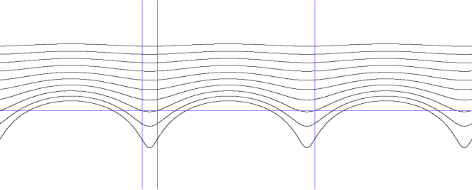
Figure 2. The black curves are the images of some horizontal lines by $Y_{r}$. The vertical lines in blue, from left to right, are the images of the vertical lines $\operatorname{Re}w=-1$, $\operatorname{Re}w=0$, and $\operatorname{Re}w=1/\alpha$, under $Y_{r}$. Here, $r=1/(10+1/(1+1/(1+\dots)))$.

Lemma 3.1.

For every $r\in(0,1/2]$, $Y_{r}$ is injective on $\overline{{\mathbb{H}}^{\prime}}$ and its image is contained in ${\mathbb{H}}^{\prime}$.

Proof.

Using $0\leq r\leq 1/2$, $3\leq\pi\leq 4$, and $10\leq e^{12/5}$, we obtain

$$\log(4+3\pi r)+2\pi r\leq\log(e^{12/5})+\pi\leq\log e^{4\pi/5}+\pi\leq 9\pi/5.$$

Thus, for all $r\in[0,1/2]$, we have $e^{9\pi/5}\geq(4+3\pi r)e^{2\pi r}$, and hence

$$\pi e^{\pi r}(e^{9\pi/5}-(4+3\pi r)e^{2\pi r}))\geq 0.$$

Now, fix $r\in[0,1/2]$. One may integrate the above inequality from $0$ to $r$, to obtain

$$e^{9\pi/5}(e^{\pi r}-1)-(\pi r+1)e^{3\pi r}+1\geq 0.$$

This implies that for all $r\in(0,1/2]$,

(3.1) $$\frac{e^{\pi r}-1}{(\pi r+1)e^{3\pi r}-1}\geq e^{-9\pi/5}.$$

On the other hand, for $w\in\overline{{\mathbb{H}}^{\prime}}$, by the triangle inequality,

$$|e^{-3\pi r}-e^{-\pi ri}e^{-2\pi riw}|\geq|e^{-\pi ri}e^{-2\pi riw}|-|e^{-3\pi r}|\geq e^{-2\pi r}-e^{-3\pi r},$$

and

$$|e^{-3\pi r}-e^{\pi ri}|\leq|e^{-3\pi r}-1|+|1-e^{\pi ri}|\leq(1-e^{-3\pi r})+\pi r.$$

Combining the above three inequalities, we obtain

$$\left|\frac{e^{-3\pi r}-e^{-\pi ri}e^{-2\pi riw}}{e^{-3\pi r}-e^{\pi ri}}\right|\geq\frac{e^{-2\pi r}-e^{-3\pi r}}{\pi r+1-e^{-3\pi r}}=\frac{e^{\pi r}-1}{(\pi r+1)e^{3\pi r}-1}\geq e^{-9\pi/5}.$$

This implies that for all $w\in{\mathbb{H}}^{\prime}$ we have

$$\operatorname{Im}Y_{r}(w)\geq\frac{1}{2\pi}\log e^{-9\pi/5}>-1.$$

In particular, $Y_{r}$ is well-defined, and maps $\overline{{\mathbb{H}}^{\prime}}$ into ${\mathbb{H}}^{\prime}$.

Let $w_{1}\neq w_{2}$ be arbitrary points in $\overline{{\mathbb{H}}^{\prime}}$. If $\operatorname{Re}w_{1}\neq\operatorname{Re}w_{2}$, then $\operatorname{Re}Y_{r}(w_{1})\neq\operatorname{Re}Y_{r}(w_{2})$. If $\operatorname{Re}w_{1}=\operatorname{Re}w_{2}$ but $\operatorname{Im}w_{1}\neq\operatorname{Im}w_{2}$, then

$$|e^{-3\pi r}-e^{-\pi ri}e^{-2\pi riw_{1}}|\neq|e^{-3\pi r}-e^{-\pi ri}e^{-2\pi riw_{2}}|.$$

This implies that $\operatorname{Im}Y_{r}(w_{1})\neq\operatorname{Im}Y_{r}(w_{2})$. These show that $Y_{r}$ is injective. ∎

Lemma 3.2.

For every $r\in(0,1/2)$, we have

• for every $w\in\overline{{\mathbb{H}}^{\prime}}$,

  $$Y_{r}(w+1/r)=Y_{r}(w)+1$$

• for every $t\geq-1$,

  $$Y_{r}(it+1/r-1)=Y_{r}(it)+1-r.$$

Proof.

Part (i) of the lemma readily follows from the formula defining $Y_{r}$.

To prove part (ii) of the lemma, first note that

$$\big{|}e^{-3\pi r}-e^{-\pi ri}e^{-2\pi ri(it+1/r-1)}\big{|} =\big{|}e^{-3\pi r}-e^{-\pi ri}e^{2\pi rt}e^{2\pi ri}\big{|}$$

$$=\big{|}e^{-3\pi r}-e^{\pi ri}e^{2\pi rt}\big{|}=\big{|}e^{-3\pi r}-e^{-\pi ri}e^{2\pi rt}\big{|}.$$

Above, the first and second “$=$” are simple multiplications of complex numbers, while for the third “$=$” we have used that $|x-z|=|x-\overline{z}|$, for real $x$ and complex $z$. Thus,

$$Y_{r}(it+1/r-1)=r(1/r-1)+\frac{i}{2\pi}\log\Big{|}\frac{e^{-3\pi r}-e^{-\pi ri}e^{2\pi rt}}{e^{-3\pi r}-e^{\pi ri}}\Big{|}=(1-r)+Y_{r}(it).\qed$$

Lemma 3.3.

For every $r\in(0,1/2)$, and every $w_{1},w_{2}$ in $\overline{{\mathbb{H}}^{\prime}}$, we have

$$|Y_{r}(w_{1})-Y_{r}(w_{2})|\leq 0.9|w_{1}-w_{2}|.$$

The precise contraction factor $0.9$ in the above lemma is not crucial; any constant less than $1$ suffices.

Proof.

Let $g(w)=(e^{-3\pi r}-e^{-\pi ri}e^{-2\pi riw})(e^{-3\pi r}-e^{\pi ri}e^{2\pi ri\overline{w}})$. Then, $g(w)$ is of the form $\zeta\overline{\zeta}$, for some $\zeta\in{\mathbb{C}}$, and hence it produces positive real values for $w\in\overline{{\mathbb{H}}^{\prime}}$. We have

$$\partial g(w)/\partial w=2\pi rie^{-\pi ri}e^{-2\pi riw}(e^{-3\pi r}-e^{\pi ri}e^{2\pi ri\overline{w}}),$$

and

$$\partial g(w)/\partial\overline{w}=-2\pi rie^{\pi ri}e^{2\pi ri\overline{w}}(e^{-3\pi r}-e^{-\pi ri}e^{-2\pi riw}).$$

Therefore, by the complex chain rule,

$$\frac{\partial}{\partial w}\big{(}\log g(w)\big{)}=\frac{1}{g(w)}\frac{\partial g}{\partial w}=\frac{2\pi rie^{-\pi ri}e^{-2\pi riw}}{e^{-3\pi r}-e^{-\pi ri}e^{-2\pi riw}}=\frac{2\pi ri}{e^{-3\pi r}e^{\pi ri}e^{2\pi riw}-1},$$

and

$$\frac{\partial}{\partial\overline{w}}\big{(}\log g(w)\big{)}=\frac{1}{g(w)}\frac{\partial g}{\partial\overline{w}}=\frac{-2\pi rie^{\pi ri}e^{2\pi ri\overline{w}}}{e^{-3\pi r}-e^{\pi ri}e^{2\pi ri\overline{w}}}=\frac{-2\pi ri}{e^{-3\pi r}e^{-\pi ri}e^{-2\pi ri\overline{w}}-1}.$$

We rewrite $Y_{r}$ in the following form

$$Y_{r}(w)=r\cdot\frac{w+\overline{w}}{2}+\frac{i}{2\pi}\cdot\frac{1}{2}\log g(w)-\frac{i}{2\pi}\log|e^{-3\pi r}-e^{\pi ri}|.$$

Then, by the above calculations,

$$\frac{\partial Y_{r}}{\partial w}(w)=\frac{r}{2}+\frac{i}{4\pi}\cdot\frac{2\pi ri}{e^{-3\pi r}e^{\pi ri}e^{2\pi riw}-1}=\frac{r}{2}\Big{(}1-\frac{1}{e^{-3\pi r}e^{\pi ri}e^{2\pi riw}-1}\Big{)},$$

and

$$\frac{\partial Y_{r}}{\partial\overline{w}}(w)=\frac{r}{2}+\frac{i}{4\pi}\cdot\frac{-2\pi ri}{e^{-3\pi r}e^{-\pi ri}e^{-2\pi ri\overline{w}}-1}=\frac{r}{2}\Big{(}1+\frac{1}{e^{-3\pi r}e^{-\pi ri}e^{-2\pi ri\overline{w}}-1}\Big{)}.$$

Let $\xi=e^{-3\pi r}e^{\pi ri}e^{2\pi riw}$. For $w\in\overline{{\mathbb{H}}^{\prime}}$, $|\xi|\leq e^{-\pi r}$. For the maximum size of the directional derivative of $Y_{r}$ we have

$$\max_{\theta\in[0,2\pi]}\big{|}\operatorname{D}Y_{r}(w)\cdot e^{i\theta}\big{|} =\Big{|}\frac{\partial Y_{r}}{\partial w}(w)\Big{|}+\Big{|}\frac{\partial Y_{r}}{\partial\overline{w}}(w)\Big{|}$$

$$\leq\frac{r}{2}\cdot\Big{|}1-\frac{1}{\xi-1}\Big{|}+\frac{r}{2}\cdot\Big{|}1+\frac{1}{\overline{\xi}-1}\Big{|}$$

$$\leq\frac{r}{2}\cdot\frac{2+e^{-\pi r}}{1-e^{-\pi r}}+\frac{r}{2}\cdot\frac{e^{-\pi r}}{1-e^{-\pi r}}=r\cdot\frac{e^{\pi r}+1}{e^{\pi r}-1}.$$

For $r\geq 0$, $e^{\pi r}-1\geq\pi r+\pi^{2}r^{2}/2$, (the first two terms of the Taylor series with positive terms). This gives us

$$r\cdot\frac{e^{\pi r}+1}{e^{\pi r}-1}=r\left(1+\frac{2}{e^{\pi r}-1}\right)\leq r\left(1+\frac{2}{\pi r+\pi^{2}r^{2}/2}\right)=\frac{2\pi r+\pi^{2}r^{2}+4}{2\pi+\pi^{2}r}.$$

The last function in the above equation is increasing on $(0,1/2)$, because it has a non-negative derivative $(4\pi r+\pi^{2}r^{2})/(2+\pi r)^{2}$. Then, it is bounded by its value at $1/2$, which, using $\pi\geq 3$, gives us

$$\frac{2\pi r+\pi^{2}r^{2}+4}{2\pi+\pi^{2}r}\leq\frac{\pi+\pi^{2}/4+4}{2\pi+\pi^{2}/2}=\frac{1}{2}+\frac{4}{2\pi+\pi^{2}/2}\leq\frac{1}{2}+\frac{4}{6+4}=\frac{9}{10}.\qed$$

Recall the map $h_{r}$ defined in Sec. 2 , that is, a diffeomorphism from ${\mathbb{R}}$ onto $(0,+\infty)$. The map $Y_{r}$ closely traces the behaviour of $h_{r}^{-1}$. By some elementary calculations, one can see that for all $r\in(0,1/2]$ and all $y\geq 1$, we have

(3.2) $$|2\pi\operatorname{Im}Y_{r}(iy/(2\pi))-h_{r}^{-1}(y)|\leq\pi.$$

Also, $Y_{r}$ captures the remarkable functional relation for the Brjuno function. By elementary calculations, one can see that for all $r\in(0,1/2]$, and all $y\geq 0$, we have

(3.3) $$2\pi ry+\log(1/r)-4\leq 2\pi\operatorname{Im}Y_{r}(1/(2r)+iy)\leq 2\pi ry+\log(1/r)+2.$$

Compare this with the second functional equation in (2.6). In particular, $Y_{r}(1/(2r))$ is uniformly close to $1/2+i(\log 1/r)/(2\pi)$.

3.2. The straight topological model

Recall the sequence $\{\alpha_{n}\}_{n=0}^{\infty}$ introduced in Sec. 2.1. Let $s(w)=\overline{w}$ denote the complex conjugation map. For $n\geq 0$ we define the maps $Y_{n}:\overline{\mathbb{H}^{\prime}}\to\mathbb{H}^{\prime}$ as

(3.4) $$Y_{n}(w)=\begin{cases}Y_{\alpha_{n}}(w)&\text{if }\varepsilon_{n}=-1,\\ -s\circ Y_{\alpha_{n}}(w)&\text{if }\varepsilon_{n}=+1.\end{cases}$$

Each $Y_{n}$ is either orientation preserving or reversing, depending on the sign of $\varepsilon_{n}$. For $n\geq 0$, we have

(3.5) $$Y_{n}(i[-1,+\infty))\subset i(-1,+\infty),\;Y_{n}(0)=0.$$

It follows from Lem 3.2 that for all $n\geq 0$ and all $w\in\overline{{\mathbb{H}}^{\prime}}$,

(3.6) $$Y_{n}(w+1/\alpha_{n})=\begin{cases}Y_{n}(w)+1&\text{if }\varepsilon_{n}=-1,\\ Y_{n}(w)-1&\text{if }\varepsilon_{n}=+1.\end{cases}$$

Also, by the same lemma, for all $n\geq 0$, and all $t\geq-1$,

(3.7) $$Y_{n}(it+1/\alpha_{n}-1)=\begin{cases}Y_{n}(it)+(1-\alpha_{n})&\text{if }\varepsilon_{n}=-1,\\ Y_{n}(it)+(\alpha_{n}-1)&\text{if }\varepsilon_{n}=+1.\end{cases}$$

Lem 3.3 implies that for all $n\geq 0$ and all $w_{1},w_{2}$ in $\overline{{\mathbb{H}}^{\prime}}$, we have

(3.8) $$|Y_{n}(w_{1})-Y_{n}(w_{2})|\leq 0.9|w_{1}-w_{2}|.$$

For $n\geq 0$ let

(3.9) $$\begin{gathered}M_{n}^{0}=\{w\in\overline{{\mathbb{H}}^{\prime}}\mid\operatorname{Re}w\in[0,1/\alpha_{n}]\},\\ J_{n}^{0}=\{w\in M_{n}^{0}\mid\operatorname{Re}w\in[1/\alpha_{n}-1,1/\alpha_{n}]\},\\ K_{n}^{0}=\{w\in M_{n}^{0}\mid\operatorname{Re}w\in[0,1/\alpha_{n}-1]\}.\end{gathered}$$

We inductively defined the sets $M_{n}^{j}$, $J_{n}^{j}$, and $K_{n}^{j}$, for $j\geq 1$ and $n\geq 0$. Assume that $M_{n}^{j}$, $J_{n}^{j}$, and $K_{n}^{j}$ are defined for some $j\geq 0$ and all $n\geq 0$. We define these sets for $j+1$ and all $n\geq 0$ as follows. Fix an arbitrary $n\geq 0$. If $\varepsilon_{n+1}=-1$, let

(3.10) $$M_{n}^{j+1}=\bigcup_{l=0}^{a_{n}-2}\big{(}Y_{n+1}(M_{n+1}^{j})+l\big{)}\bigcup\big{(}Y_{n+1}(K_{n+1}^{j})+a_{n}-1\big{)}.$$

If $\varepsilon_{n+1}=+1$, let

(3.11) $$M_{n}^{j+1}=\bigcup_{l=1}^{a_{n}}\big{(}Y_{n+1}(M_{n+1}^{j})+l\big{)}\bigcup\big{(}Y_{n+1}(J_{n+1}^{j})+a_{n}+1\big{)}.$$

Regardless of the sign of $\varepsilon_{n+1}$, define

$$J_{n}^{j+1}=\{w\in M_{n}^{j+1}\mid\operatorname{Re}w\in[1/\alpha_{n}-1,1/\alpha_{n}]\},$$

$$K_{n}^{j+1}=\{w\in M_{n}^{j+1}\mid\operatorname{Re}w\in[0,1/\alpha_{n}-1]\}.$$

Fig 3 presents two generations of these domains.

Figure 3. In the left hand column $\varepsilon_{n}=-1$ and in the right hand column $\varepsilon_{n}=+1$. The sets $K_{n}^{0}$ and $J_{n}^{0}$ are on the lower row, and the set $M_{n-1}^{1}$ is on the upper row.

For all $n\geq 0$ and $j\geq 0$, the sets $M_{n}^{j}$, $J_{n}^{j}$, and $K_{n}^{j}$ are closed and connected subsets of ${\mathbb{C}}$, and are bounded by piece-wise analytic curves. Moreover,

$$\{\operatorname{Re}w\mid w\in M_{n}^{j}\}=[0,1/\alpha_{n}].$$

The functional relations in (3.6) and (3.7) allow us to align together the pieces in the unions (3.10) and (3.11). More precisely, we have the following property of the sets $M_{n}^{j}$.

Corollary 3.4.

For every $n\geq 0$ and $j\geq 0$, the following hold:

• for all $w\in\mathbb{C}$ satisfying $\operatorname{Re}w\in[0,1/\alpha_{n}-1]$, $w\in M_{n}^{j}$ if and only if $w+1\in M_{n}^{j}$;

• for all $t\in\mathbb{R}$, $it\in M_{n}^{j}$ if and only if $it+1/\alpha_{n}\in M_{n}^{j}$.

Recall that $\alpha_{-1}=+1$. Let $M_{-1}^{0}=\{w\in\overline{{\mathbb{H}}^{\prime}}\mid\operatorname{Re}w\in[0,1/\alpha_{-1}]\}$, and for $j\geq 1$, consider the sets

$$M_{-1}^{j}=Y_{0}(M_{0}^{j-1})+(\varepsilon_{0}+1)/2.$$

By Lem 3.1, $M_{n}^{1}\subset M_{n}^{0}$, for $n\geq-1$. By an inductive argument, this implies that for all $n\geq-1$ and all $j\geq 0$,

(3.12) $$M_{n}^{j+1}\subset M_{n}^{j}.$$

For $n\geq-1$, we define

$$M_{n}=\bigcap_{j\geq 1}M_{n}^{j}.$$

Each $M_{n}$ consists of closed half-infinite vertical lines tending to $+i\infty$. However, $M_{n}$ may or may not be connected. We note that $\operatorname{Re}M_{-1}\subset[0,1]$. Indeed, by Cor 3.4, for real $t$, $it\in M_{-1}$ if and only if $(it+1)\in M_{-1}$. We may define the set

(3.13) $$\begin{gathered}A_{\alpha}=\left\{s(e^{2\pi iw})\mid w\in M_{-1},\operatorname{Im}w\leq p_{-1}(\operatorname{Re}w)\right\},\quad\text{if }\alpha\in{\mathscr{B}},\\ A_{\alpha}=\left\{s(e^{2\pi iw})\mid w\in M_{-1}\right\}\cup\left\{0\right\},\quad\text{if }\alpha\notin{\mathscr{B}}.\end{gathered}$$

The set $A_{\alpha}$ is our topological model for the post-critical set. It is defined for irrational values of $\alpha$, and depends only on the arithmetic of $\alpha$.

3.3. Hairy Cantor sets and Cantor bouquets

We shall describe the topology of $A_{\alpha}$ in Section 3.4.

The simplest scenario is when $A_{\alpha}$ is a Jordan curve. However, there are other possibilities, which we present below.

A Cantor bouquet is any subset of the plane which is ambiently homeomorphic to a set of the form

$$\{re^{2\pi i\theta}\in{\mathbb{C}}\mid 0\leq\theta\leq 1,0\leq r\leq R(\theta)\}$$

where $R:{\mathbb{R}}/{\mathbb{Z}}\to[0,1]$ satisfies the following:

• $R=0$ on a dense subset of ${\mathbb{R}}/{\mathbb{Z}}$, and $R>0$ on a dense subset of ${\mathbb{R}}/{\mathbb{Z}}$,

• for each $\theta_{0}\in{\mathbb{R}}/{\mathbb{Z}}$ we have

  $$\limsup_{\theta\to\theta_{0}^{+}}R(\theta)=R(\theta_{0})=\limsup_{\theta\to\theta_{0}^{-}}R(\theta).$$

A one-sided hairy Jordan curve is any subset of the plane which is ambiently homeomorphic to a set of the form

$$\{re^{2\pi i\theta}\in{\mathbb{C}}\mid 0\leq\theta\leq 1,1\leq r\leq 1+R(\theta)\}$$

where $R:{\mathbb{R}}/{\mathbb{Z}}\to[0,1]$ satisfies properties (a) and (b) in the above definition.

Remark 3.5.

The Cantor bouquet and one-sided hairy Jordan curve enjoy similar topological features as the standard Cantor set. Under an additional mild condition (topological smoothness) they are uniquely characterised by some topological axioms, see [AO93].

An alternative approach for building a topological model for $\Lambda(f)$ was studied by Buff and Chéritat in 2009 [BC09]. In their model, they use rational approximation of $\alpha$, and some conformal changes of coordinates, to build topological models for some invariant sets for maps with a parabolic fixed point. Then, the model for irrational values of $\alpha$ is obtained from taking Hausdorff limits of those objects. Naturally, one looses control along the limit. This has been the main reason behind the construction in [Che21], which is summarised here.

3.4. Topology of the model

Recall that the sets $M_{n}^{j}$ and $M_{n}$ consist of closed half-infinite vertical lines. Thus, each of these sets lies above the graph of a function, which may be conveniently used to explain the topological structure of the sets $M_{n}$. For $n\geq-1$, and $j\geq 0$, define the function $b_{n}^{j}:[0,1/\alpha_{n}]\to[-1,+\infty)$ as

(3.14) $$b_{n}^{j}(x)=\min\{y\mid x+iy\in M_{n}^{j}\}.$$

Since each $Y_{n}$ preserves vertical lines, it follows that

$$M_{n}^{j}=\{w\in{\mathbb{C}}\mid 0\leq\operatorname{Re}w\leq 1/\alpha_{n},\operatorname{Im}w\geq b_{n}^{j}(\operatorname{Re}w)\}.$$

It follows from the definition of the sets $M_{n}^{j}$, and the functional equations (3.6)–(3.7), one may see that for all $n\geq-1$ and $j\geq 0$, $b_{n}^{j}:[0,1/\alpha_{n}]\to[-1,+\infty)$ is continuous. Moreover, by (3.12), we must have $b_{n}^{j+1}\geq b_{n}^{j}$ on $[0,1/\alpha_{n}]$. Thus, for $n\geq-1$, we may define $b_{n}:[0,1/\alpha_{n}]\to[-1,+\infty]$ as

$$b_{n}(x)=\lim_{j\to+\infty}b_{n}^{j}(x)=\sup_{j\geq 0}b_{n}^{j}(x).$$

Note that $b_{n}$ is allowed to attain $+\infty$. Evidently, the function $b_{n}$ describes the set $M_{n}$ as follow

(3.15) $$M_{n}=\{w\in{\mathbb{C}}\mid 0\leq\operatorname{Re}w\leq 1/\alpha_{n},\operatorname{Im}w\geq b_{n}(\operatorname{Re}w)\}.$$

By Cor 3.4, $b_{n}^{j}(0)=b_{n}^{j}(1/\alpha_{n})$, and $b_{n}^{j}(x+1)=b_{n}^{j}(x)$ for all $x\in[0,1/\alpha_{n}-1]$. Taking limits as $j\to+\infty$, we conclude that for all $n\geq-1$

(3.16) $$b_{n}(0)=b_{n}(1/\alpha_{n}),\quad\text{and}\quad b_{n}(x+1)=b_{n}(x),\,\forall x\in[0,1/\alpha_{n}-1].$$

The collection of the functions $b_{n}^{j}$ and $b_{n}$ enjoy an equivariant relation induced by the maps $Y_{n}$. That is, the graph of $b_{n}$ is obtained from the graph of $b_{n+1}$ by applying the map $Y_{n+1}$ and its translations. Each of the maps $Y_{n}$ exhibits two distinct behaviour. Above the horizontal line $\operatorname{Im}w=1/\alpha_{n}$ it nearly acts as the linear map multiplication by $\alpha_{n}$. Below that horizontal line, there is a logarithmic behaviour in imaginary direction. The functions $b_{n}$ mostly capture the behaviour of the collection of maps $Y_{n}$ near the lower end of their domains. There is another collection of functions which captures the behaviour of the collection of maps $Y_{n}$ for the top regions. Indeed, near the bottom end of the top regions. As we shall see in a moment, these are only relevant for Brjuno values of $\alpha$. We present these functions below.

Assume that $\alpha$ is a Brjuno number. For $n\geq-1$ and $j\geq 0$ we inductively define the functions

$$p_{n}^{j}:[0,1/\alpha_{n}]\to[-1,+\infty).$$

For all $n\geq-1$, we set $p_{n}^{0}\equiv({\mathcal{B}}(\alpha_{n+1})+5\pi)/(2\pi)$. Assuming that $p_{n}^{j}$ is defined for some $j\geq 0$ and all $n\geq-1$, we define $p_{n}^{j+1}$ on $[0,1/\alpha_{n}]$ as follows. For $x_{n}\in[0,1/\alpha_{n}]$, we find $x_{n+1}\in[0,1/\alpha_{n+1}]$ and $l_{n}\in{\mathbb{Z}}$ such that $-\varepsilon_{n+1}\alpha_{n+1}x_{n+1}=x_{n}-l_{n}$, and define

$$p_{n}^{j+1}(x_{n})=\operatorname{Im}Y_{n+1}\big{(}x_{n+1}+ip_{n+1}^{j}(x_{n+1})\big{)}.$$

In other words, the graph of $p_{n}^{j+1}$ is obtained from applying $Y_{n+1}$ to the graph of $p_{n+1}^{j}$ on $[0,1/\alpha_{n+1}]$, and translating it by some integers.

Evidently, for all $n\geq-1$ and all $j\geq 0$, we have $p_{n}^{j+1}(x+1)=p_{n}^{j+1}(x)$, for $x\in[0,1/\alpha_{n}-1]$. Moreover, it follows from (3.6) and (3.7) that each $p_{n}^{j}:[0,1/\alpha_{n}]\to{\mathbb{R}}$ is continuous, and $p_{n}^{j}(0)=p_{n}^{j}(1/\alpha_{n})$.

Because of the choice of the constant $(5\pi)/(2\pi)$ in the definition of $p_{n}^{0}$, some calculations of the formula for $Y_{n}$ may be used to show that $p_{n}^{1}\leq p_{n}^{0}$, for all $n\geq-1$. Then, using an induction argument, one may show that for all $n\geq-1$ and $j\geq 0$ we have

$$p_{n}^{j+1}(x)\leq p_{n}^{j}(x),\quad\forall x\in[0,1/\alpha_{n}].$$

Therefore, we may define the functions

$$p_{n}(x)=\lim_{j\to+\infty}p_{n}^{j}(x),\quad\forall x\in[0,1/\alpha_{n}].$$

A main difference with the functions $b_{n}^{j}$ is that the convergence in the above equation is uniform on all of $[0,1/\alpha_{n}]$. This is mainly because the maps $Y_{n}$ behave better near the top end of $M_{n}^{0}$; they are close to multiplication by $\alpha_{n}$. In particular, we conclude that for $n\geq-1$, $p_{n}:[0,1/\alpha_{n}]\to[1,+\infty)$ is continuous. Moreover, the functional relations for $p_{n}^{j}$ imply that

(3.17) $$p_{n}(0)=p_{n}(1/\alpha_{n}),\quad p_{n}(x)=p_{n}(x+1),\forall x\in[0,1/\alpha_{n}-1].$$

By definition, $p_{n}^{0}\geq b_{n}^{0}$, for all $n\geq-1$. Since the graphs of $b_{n+1}^{0}$ and $p_{n+1}^{0}$ are mapped to the graphs of $b_{n}^{1}$ and $p_{n}^{1}$, respectively, under $Y_{n+1}$ and its translations, we must have $p_{n}^{1}\geq b_{n}^{1}$, for all $n\geq-1$. By induction, this implies that for all $n\geq-1$ and all $j\geq 0$, $p_{n}^{j}(x)\geq b_{n}^{j}(x)$, for all $x\in[0,1/\alpha_{n}]$. In particular,

(3.18) $$p_{n}(x)\geq b_{n}(x),\quad\forall x\in[0,1/\alpha_{n}].$$

Because for all $\alpha\in\mathbb{R}\setminus\mathbb{Q}$, $Y_{n}(0)=0$ for all $n\geq 0$, and all of $Y_{n}$ are uniformly contracting, one may see that for all $n\geq-1$,

(3.19) $$b_{n}(0)=0.$$

Employing the periodicity of the functions $b_{n}$, and their equivariant relations induced from the maps $Y_{n}$, one concludes that or every $n\geq-1$, $b_{n}<+\infty$ holds on a dense subset of $[0,1/\alpha_{n}]$. In the same fashion, if some $b_{m}$ attains $+\infty$ at a single point, then every $b_{n}$ attains $+\infty$ on a dense subset of $[0,1/\alpha_{n}]$. The question of whether this happens or not depends on the arithmetic of $\alpha$. Indeed, because of the functional relations in (2.6) and (3.3), an explicit calculation show that for all $n\geq-1$ we have

(3.20) $$\Big{|}2\pi\sup_{x\in[0,1/\alpha_{n}]}b_{n}(x)-{\mathcal{B}}(\alpha_{n+1})\Big{|}\leq 5\pi.$$

In the above relation, $\infty-\infty$ is assumed to be $0$. In particular, if $\alpha$ is a Brjuno number, every $b_{n}$ is bounded, and if $\alpha$ is not a Brjuno number, every $b_{n}$ attains $+\infty$ on a dense set of points.

The estimate in (3.20) also implies that when $\alpha$ is a Brjuno number, $b_{n}$ is uniformly close to $p_{n}$ at some points. By the uniform contraction of the maps $Y_{n}$, and the equivariant property of the collections of functions $b_{n}$ and $p_{n}$, we must have $p_{n}(x)=b_{n}(x)$ on a dense set of points in $[0,1/\alpha_{n}]$. Alternatively, one may see that these equalities occur due to the particular contracting factor of each map $Y_{n}$ near the vertical line $\operatorname{Re}w=1/(2\alpha_{n})$. Among the vertical lines in the domain of $Y_{n}$, the least amount of contraction occurs near the vertical line $\operatorname{Re}w=0$. So, $0$ is the least likely place where $b_{n}$ and $p_{n}$ become equal. Indeed, the answer to this question depends on the arithmetic of $\alpha$ as we explain below.

Because of the uniform contraction of the maps $h_{\alpha_{n}}$, the criterion for the Herman numbers is stable under uniform changes to the maps $h_{\alpha_{n}}$. More precisely, if one replaces $h_{\alpha_{n}}$ by uniformly nearby maps, say $Y_{n}^{-1}$, the corresponding set of rotation numbers stays the same. Indeed, one may employ the estimate in (3.2) to show that for integers $m>n\geq 0$ and $y\in(1,+\infty)$,

$$\big{|}2\pi\operatorname{Im}Y_{n}\circ\dots\circ Y_{m}(iy/(2\pi))-h_{\alpha_{n}}^{-1}\circ\dots\circ h_{\alpha_{m}}^{-1}(y)\big{|}\leq 10\pi,$$

provided $h_{\alpha_{n}}^{-1}\circ\dots\circ h_{\alpha_{m}}^{-1}(y)$ is defined. The uniform estimate above, and the uniform contraction of the maps $Y_{n}$ may be used to show that an irrational number $\alpha$ belongs to ${\mathscr{H}}$, if and only if, for all $x>0$ there is $m\geq 1$ such that

$$\operatorname{Im}Y_{0}\circ\dots\circ Y_{m-1}(i{\mathcal{B}}(\alpha_{m})/(2\pi))\leq x.$$

In particular, this implies that for Brjuno values of $\alpha$, $\alpha$ is a Herman number if and only if $p_{n}(0)=0$ for all $n\geq-1$. Combining with earlier arguments, we conclude that when $\alpha$ is a Herman number, we have $b_{n}\equiv p_{n}$, and when $\alpha$ is a Brjuno but not a Herman number, $b_{n}<p_{n}$ holds on a dense subset of $[0,1/\alpha_{n}]$.

Because each $M_{n}$ is a closed set, for every $x\in[0,1/\alpha_{n})$, $\liminf_{s\to x^{+}}b_{n}(s)\geq b_{n}(x)$, and for all $x\in(0,1/\alpha_{n}]$, $\liminf_{s\to x^{-}}b_{n}(s)\geq b_{n}(x)$. In fact, both of “$\geq$” are “$=$”. That is because, for large values of $m$, $b_{n+m}$ is periodic of period $+1$. Employing the equivariant property of the maps $b_{j}$, and the uniform contraction of the maps $Y_{j}$, one may obtain a sequence of points on the graph of $b_{n}$ which converges to $(x,b_{n}(x))$. With a detailed analysis of the trajectories of points in the tower of maps $Y_{j}$, one can see that this can be done from both sides. These relations imply the property (b) in the definition of the hairy Jordan curve and the Cantor bouquet.

Combining the properties we summarised in this section, we obtain the following classification.

Theorem 3.6 ([Che21]).

Let $\alpha$ be an irrational number. We have,

• if $\alpha$ is a Herman number, then $A_{\alpha}$ is a closed Jordan curve;

• if $\alpha$ is a Brjuno but not a Herman number, then $A_{\alpha}$ is a one-sided hairy Jordan curve;

• if $\alpha$ is not a Brjuno number, then $A_{\alpha}$ is a Cantor Bouquet.

3.5. Dynamics on the topological model

In this section we introduce a map

(3.21) $$T_{\alpha}:A_{\alpha}\to A_{\alpha},$$

which serves as the model for the map $f$ on $\Lambda(f)$. We summarise the dynamical properties of this map which were obtained in [Che21].

Let us fix $\alpha\in{\mathbb{R}}\setminus{\mathbb{Q}}$, and let $M_{-1}$ be the corresponding topological model defined in Sec. 3.2. Given $w_{-1}\in M_{-1}$, we inductively identify the integers $l_{i}$, and then the points $w_{i+1}\in M_{i+1}$ such that

(3.22) $$\begin{gathered}0\leq\operatorname{Re}(w_{i}-l_{i})<1,\quad\text{if }\varepsilon_{i+1}=-1,\\ \quad-1<\operatorname{Re}(w_{i}-l_{i})\leq 0,\quad\text{if }\varepsilon_{i+1}=+1,\\ \quad Y_{i+1}(w_{i+1})+l_{i}=w_{i}.\end{gathered}$$

It follows that for all $n\geq 0$, we have

(3.23) $$w_{-1}=(Y_{0}+l_{-1})\circ(Y_{1}+l_{0})\circ\dots\circ(Y_{n}+1_{n-1})(w_{n}).$$

Also, by the definition of $M_{i}$ in (3.10) and (3.11), for all $i\geq 0$,

(3.24) $$0\leq l_{i}\leq a_{i}+\varepsilon_{i+1},\quad\text{ and }\quad 0\leq\operatorname{Re}w_{i}<1/\alpha_{i}.$$

We refer to the sequence $(w_{i};l_{i})_{i\geq-1}$ as the trajectory of $w_{-1}$, with respect to $\alpha$, or simply, as the trajectory of $w_{-1}$, when it is clear from the context what irrational number is used.

Consider the map

(3.25) $$\tilde{T}_{\alpha}:M_{-1}\to M_{-1},$$

defined as follows. For an arbitrary point $w_{-1}$ in $M_{-1}$ with trajectory $(w_{i};l_{i})_{i\geq-1}$,

• if there is $n\geq 0$ such that $w_{n}\in K_{n}$, and for all $0\leq i\leq n-1$, $w_{i}\in M_{i}\setminus K_{i}$, then

  $$\tilde{T}_{\alpha}(w_{-1})=\left(Y_{0}+\frac{\varepsilon_{0}+1}{2}\right)\circ\left(Y_{1}+\frac{\varepsilon_{1}+1}{2}\right)\circ\cdots\circ\left(Y_{n}+\frac{\varepsilon_{n}+1}{2}\right)(w_{n}+1);$$

• if for all $n\geq 0$, $w_{n}\in M_{n}\setminus K_{n}$, then

  $$\tilde{T}_{\alpha}(w_{-1})=\lim_{n\to+\infty}\left(Y_{0}+\frac{\varepsilon_{0}+1}{2}\right)\circ\left(Y_{1}+\frac{\varepsilon_{1}+1}{2}\right)\circ\cdots\circ\left(Y_{n}+\frac{\varepsilon_{n}+1}{2}\right)(w_{n}+1-1/\alpha_{n}).$$

Evidently, item (i) leads to continuous maps on pieces of $M_{-1}$. There might be a vertical half-infinite line where item (ii) above applies. On that set, the uniform contraction of the maps $Y_{j}$ implies that the maps converge to a well-defined map. It follows from the functional equations (3.6) and (3.7) that these pieces match together and produce a well-define homeomorphism

$$\tilde{T}_{\alpha}:M_{-1}/{\mathbb{Z}}\to M_{-1}/{\mathbb{Z}}.$$

One may compare the above definition of the map $\tilde{T}_{\alpha}$ to the action of the map $f$ on its renormalisation tower in Sec. 7.4. By the definition of $A_{\alpha}$ in (3.13), $\tilde{T}_{\alpha}$ induces a homeomorphism

$$T_{\alpha}:A_{\alpha}\to A_{\alpha}.$$

Recall that a map $f:X\to X$, of a topological space $X$, is called topologically recurrent, if for every $x\in X$ there is a strictly increasing sequence of positive integers $(m_{i})_{i\geq 0}$ such that $f^{\circ{m_{i}}}(x)\to x$ as $i\to+\infty$. Also, recall that a set $K\subset A_{\alpha}$ is called invariant under $T_{\alpha}$, if $T_{\alpha}(K)=K=T_{\alpha}^{-1}(K)$.

Define $r_{\alpha}\in[0,1]$ according to

$$[r_{\alpha},1]=\{z\in A_{\alpha}\mid\operatorname{Im}z=0,\operatorname{Re}z\geq 0\}.$$

Below we summarise the dynamical behaviour of $T_{\alpha}$ on $A_{\alpha}$ which are obtained in [Che21].

In the next theorem, $\omega(z)$ denotes the set of accumulation points of the orbit of the point $z$.

Theorem 3.7.

For every $\alpha\in\mathbb{R}\setminus\mathbb{Q}$ the map $T_{\alpha}:A_{\alpha}\to A_{\alpha}$ satisfies the following properties.

• $T_{\alpha}:A_{\alpha}\to A_{\alpha}$ is topologically recurrent.

• The map

  $$\omega:[r_{\alpha},1]\to\{X\subseteq A_{\alpha}\mid X\text{ is non-empty, closed and invariant}\}$$

  is a homeomorphism with respect to the Hausdorff metric on the range. In particular, every non-empty closed invariant subset of $A_{\alpha}$ is equal $\omega(z)$, for some $z\in A_{\alpha}$.

• The map $\omega$ on $[r_{\alpha},1]$ is strictly increasing with respect to the linear order on $[r_{\alpha},1]$ and the inclusion on the range.

• If $\alpha$ is not a Brjuno number, for every $t\in(r_{\alpha},1]$, $\omega(t)$ is a Cantor bouquet.

• If $\alpha$ is a Brjuno number, for every $t\in(r_{\alpha},1]$, $\omega(t)$ is a hairy Jordan curve.

4. Near-parabolic renormalisation scheme

In this section we present the rear-parabolic renormalisation scheme introduced by Inou and Shishikura [IS06]. This consists of a class of maps discussed in Section 4.1, and a renormalisation operator acting on that class discussed in Section 4.2. Our presentation of the renormalisation process is slightly different from the one by Inou and Shishikura, but produces the same map.

4.1. Inou-Shishikura class of maps

Let $\hat{\mathbb{C}}$ denote the Riemann sphere. Consider the filled-in ellipse

$$E=\Big{\{}x+iy\in{\mathbb{C}}\;\Big{|}\;\Big{(}\frac{x+0.18}{1.24}\Big{)}^{2}+\Big{(}\frac{y}{1.04}\Big{)}^{2}\leq 1\Big{\}},$$

and the domain

(4.1) $$U=g(\hat{\mathbb{C}}\setminus E),\text{ where }g(z)=\frac{-4z}{(1+z)^{2}}.$$

The domain $U$ is simply connected and contains $0$.

The restriction of the polynomial $P(z)=z(1+z)^{2}$ on $U$ has a specific covering structure which plays a central role in this renormalisation scheme. The polynomial $P$ has a parabolic fixed point at $0$ with multiplier $P^{\prime}(0)=1$. It has a simple critical point at $\textup{cp}_{P}=-1/3\in U$ and a critical point of order two at $-1\in{\mathbb{C}}\setminus\overline{U}$. The critical point $-1/3$ is mapped to $\textup{cv}_{P}=-4/27\in U$, and $-1$ is mapped to $0$.

Let $\mathcal{I}\mathcal{S}$ denote the class of all maps of the form

$$h=P\circ\varphi^{-1}\!\!:U_{h}\rightarrow{\mathbb{C}}$$

where

• $\varphi\colon U\rightarrow U_{h}$ is holomorphic, one-to-one, onto; and

• $\varphi(0)=0$ and $\varphi^{\prime}(0)=1$.

By (i), every map in $\mathcal{I}\mathcal{S}$ has the same covering structure on its domain as the one of $P$ on $U$. By (ii), every map in $\mathcal{I}\mathcal{S}$ has a fixed point at $0$ with multiplier $+1$, and a unique critical point at $\textup{cp}_{h}=\varphi(-1/3)\in U_{h}$ which is mapped to $\textup{cv}_{h}=-4/27$.

For $\alpha\in{\mathbb{R}}$, let $R_{\alpha}(z)=e^{2\pi\alpha i}z$. Define

$$\mathcal{I}\mathcal{S}_{\alpha}=\{h\circ R_{\alpha}\mid h\in\mathcal{I}\mathcal{S}\}.$$

We continue to use the notation $U_{h}$ to denote the domain of definition of $h\in\mathcal{I}\mathcal{S}_{\alpha}$. That is, if $h=f\circ R_{\alpha}$ with $f\in\mathcal{I}\mathcal{S}$, then $U_{h}=R_{\alpha}^{-1}(U_{f})$.

We equip $\cup_{\alpha\in{\mathbb{R}}}\mathcal{I}\mathcal{S}_{\alpha}$ with the topology of uniform convergence on compact sets. That is, given a map $h:U_{h}\to{\mathbb{C}}$, a compact set $K\subset U_{h}$, and an $\varepsilon>0$, a neighbourhood of $h$ (in the compact-open topology) is defined as the set of maps $g\in\cup_{\alpha\in{\mathbb{R}}}\mathcal{I}\mathcal{S}_{\alpha}$ such that $K\subset U_{g}$ and for all $z\in K$ we have $|g(z)-h(z)|<\varepsilon$. There is a one-to-one correspondence between $\mathcal{I}\mathcal{S}$ and the space of normalised univalent maps on the unit disk. By the Koebe distortion theorem [Dur83, Thm 2.5], for any compact set $A\subset{\mathbb{R}}$, the set $\cup_{\alpha\in A}\mathcal{I}\mathcal{S}_{\alpha}$ is pre-compact in this topology.

We normalise the family of quadratic polynomials by placing a fixed point at $0$ and the finite critical value at $-4/27$;

$$Q_{\alpha}(z)=e^{2\pi\alpha i}z+\frac{27}{16}e^{4\pi\alpha i}z^{2}.$$

Then, $Q_{\alpha}$ has a fixed point at $0$ with multiplier $e^{2\pi\alpha i}$, and a critical point at $-8e^{-2\pi\alpha i}/27$ which is mapped to $-4/27$. We shall use the notation

$$\mathcal{Q}\mathcal{I}\mathcal{S}_{\alpha}=\mathcal{I}\mathcal{S}_{\alpha}\cup\{Q_{\alpha}\}.$$

When $h=Q_{\alpha}$, we set $U_{h}={\mathbb{C}}$.

Let $h=h_{0}\circ R_{\alpha}\in\mathcal{I}\mathcal{S}_{\alpha}$ with $h_{0}\in\mathcal{I}\mathcal{S}$ and $\alpha\in\mathbb{R}$. The map $h_{0}$ has a double fixed point at $0$. For $\alpha$ small enough and non-zero, $h$ is a small perturbation of $h_{0}$, and hence, it has a non-zero fixed point near $0$ which has split from $0$ at $\alpha=0$. We denote this fixed point by $\sigma_{h}$. It follows that $\sigma_{h}$ depends continuously on $h_{0}$ and $\alpha$, with asymptotic expansion $\sigma_{h}=-4\pi\alpha i/h_{0}^{\prime\prime}(0)+o(\alpha)$, as $\alpha$ tends to $0$. Evidently, $\sigma_{h}\rightarrow 0$ as $\alpha\rightarrow 0$.

Proposition 4.1 ([IS06]).

There is $r_{1}>0$ such that for every $h\colon U_{h}\rightarrow{\mathbb{C}}$ in $\mathcal{Q}\mathcal{I}\mathcal{S}_{\alpha}$ with $\alpha\in(0,r_{1}]$, there exist a simply connected domain ${\mathcal{P}}_{h}\subset U_{h}$ and a univalent map $\Phi_{h}\colon{\mathcal{P}}_{h}\rightarrow{\mathbb{C}}$ satisfying the following properties:

• ${\mathcal{P}}_{h}$ is bounded by piecewise smooth curves and is compactly contained in $U_{h}$;

• $\textup{cp}_{h}$, $0$, and $\sigma_{h}$ belong to the boundary of ${\mathcal{P}}_{h}$, while $\textup{cv}_{h}$ belongs to the interior of ${\mathcal{P}}_{h}$;

• $\Phi_{h}({\mathcal{P}}_{h})$ contains the set $\{w\in\mathbb{C}\mid\operatorname{Re}w\in(0,1]\}$;

• $\Phi_{h}(\textup{cv}_{h})=1$, $\operatorname{Im}\Phi_{h}(z)\rightarrow+\infty$ as $z\to 0$ in ${\mathcal{P}}_{h}$, and $\operatorname{Im}\Phi_{h}(z)\rightarrow-\infty$ as $z\to\sigma_{h}$ in ${\mathcal{P}}_{h}$;

• If $z$ and $h(z)$ belong to ${\mathcal{P}}_{h}$, then

  $$\Phi_{h}(h(z))=\Phi_{h}(z)+1;$$

• the induced map $\Phi_{h}:{\mathcal{P}}_{h}/{\sim}\to{\mathbb{C}}/{\mathbb{Z}}$, where $z\sim h(z)$, is a biholomorphism;

• $\Phi_{h}$ is unique, and depends continuously on $h$.

The class $\mathcal{I}\mathcal{S}$ is denoted by $\mathcal{F}_{1}$ in [IS06]. One may refer to Theorem 2.1 as well as Main Theorems 1 and 3 in [IS06], for further details on the above proposition. A precise value for $r_{1}$ is not known to date.

There are fundamental geometric properties of ${\mathcal{P}}_{h}$ and $\Phi_{h}$ that are crucial for applications of near-parabolic renormalisation scheme. We state these in the next proposition.

Figure 4. The domain ${\mathcal{P}}_{h}$ and the special points associated to some $h\in\mathcal{I}\mathcal{S}_{\alpha}$. The alternating coloured croissants are the pre-images of vertical strips of width one by $\Phi_{h}$.

Proposition 4.2.

There exist $r_{2}\in(0,r_{1}]$, as well as integers $c_{1}\leq 1/r_{2}-3/2$ and $c_{2}$ such that for every map $h\colon U_{h}\rightarrow{\mathbb{C}}$ in $\mathcal{Q}\mathcal{I}\mathcal{S}_{\alpha}$ with $\alpha\in(0,r_{2}]$, the domain ${\mathcal{P}}_{h}\subset U_{h}$ in Prop 4.1 may be chosen to satisfy the additional properties:

• there exists a continuous branch of argument defined on ${\mathcal{P}}_{h}$ such that

  $$\max_{w,w^{\prime}\in{\mathcal{P}}_{h}}|\arg(w)-\arg(w^{\prime})|\leq 2\pi c_{2},$$

• $\Phi_{h}({\mathcal{P}}_{h})=\{w\in{\mathbb{C}}\mid 0<\operatorname{Re}(w)<\alpha^{-1}-c_{1}\}$.

See [Che13, Prop. 2.4] or [BC12, Prop. 12] for proofs. The map $\Phi_{h}:\mathcal{P}_{h}\to{\mathbb{C}}$ is called the perturbed Fatou coordinate or simply the Fatou coordinate of $h$. See Figure 4.

4.2. Near-parabolic renormalisation operator

Let $h\colon U_{h}\rightarrow{\mathbb{C}}$ be a map in $\mathcal{Q}\mathcal{I}\mathcal{S}_{\alpha}$ with $\alpha\in(0,r_{2}]$, and let $\Phi_{h}\colon{\mathcal{P}}_{h}\rightarrow{\mathbb{C}}$ denote the Fatou coordinate of $h$ introduced in the previous section. Let

(4.2) $$\begin{gathered}A_{h}=\{z\in{\mathcal{P}}_{h}:1/2\leq\operatorname{Re}(\Phi_{h}(z))\leq 3/2\>,\>-2\leq\operatorname{Im}\Phi_{h}(z)\leq 2\},\\ B_{h}=\{z\in{\mathcal{P}}_{h}:1/2\leq\operatorname{Re}(\Phi_{h}(z))\leq 3/2\>,\>2\leq\operatorname{Im}\Phi_{h}(z)\}.\end{gathered}$$

By Prop 4.1, $\textup{cv}_{h}$ belongs to the interior of $A_{h}$ and $0$ belongs to the boundary of $B_{h}$. See Figure 5.

It follows from [IS06] (see Rem 4.4 below) that there is a positive integer $k_{h}$, depending on $h$, such that the following four properties hold:

• For every integer $k$, with $1\leq k\leq k_{h}$, there exists a unique connected component of $h^{-k}(B_{h})$ which is compactly contained in $U_{h}$ and contains $0$ on its boundary. We denote this component by $B_{h}^{-k}$.

• For every integer $k$, with $1\leq k\leq k_{h}$, there exists a unique connected component of $h^{-k}(A_{h})$ which has non-empty intersection with $B_{h}^{-k}$, and is compactly contained in $U_{h}$. This component is denoted by $A_{h}^{-k}$.

• The sets $A_{h}^{-k_{h}}$ and $B_{h}^{-k_{h}}$ are contained in

  $$\big{\{}z\in{\mathcal{P}}_{h}\mid 1/2<\operatorname{Re}\Phi_{h}(z)<1/\alpha-c_{1}\big{\}}.$$

• The maps $h:A_{h}^{-k}\to A_{h}^{-k+1}$, for $2\leq k\leq k_{h}$, and $h:B_{h}^{-k}\to B_{h}^{-k+1}$, for $1\leq k\leq k_{h}$, are one-to-one. The map $h:A_{h}^{-1}\to A_{h}$ is a degree two proper branched covering.

Assume that $k_{h}$ is the smallest positive integer for which the above properties hold. Define

$$S_{h}=A_{h}^{-k_{h}}\cup B_{h}^{-k_{h}}.$$

Proposition 4.3.

The is a constant $k\in{\mathbb{Z}}$ such that for all $h\in\mathcal{Q}\mathcal{I}\mathcal{S}$, $k_{h}\leq k$.

See [Che13] or [Che19] for the proof of the above proposition.

Figure 5. Illustration of the sets $A_{h}$, $B_{h}$,…, $A_{h}^{-k_{h}}$, $B_{h}^{-k_{h}}$, and the sector $S_{h}$. The amoeba shaped red curve denotes a large number of iterates of $\textup{cp}_{h}$ under $h$.

Since $h^{\circ{k_{h}}}:S_{h}\to A_{h}\cup B_{h}$, the composition

(4.3) $$E_{h}=\Phi_{h}\circ h^{\circ{k_{h}}}\circ\Phi_{h}^{-1}:\Phi_{h}(S_{h})\rightarrow{\mathbb{C}}$$

is a well-defined map. Moreover, by Prop 4.1-(e), $E_{h}(w+1)=E_{h}(w)+1$, when both $w$ and $w+1$ belong to the closure of $\Phi_{h}(S_{h})$.

Consider the covering map

(4.4) $$\operatorname{\mathbb{E}xp}(w)=(-4/27)e^{2\pi iw}.$$

Since $E_{h}$ commutes with the translation by $+1$, it induces via $\operatorname{\mathbb{E}xp}$ a unique map $\operatorname{\mathcal{R}}(h)$ defined on a set containing a punctured neighbourhood of $0$. Since $\operatorname{\mathcal{R}}(h)(z)\to 0$ as $z\to 0$, $0$ is a removable singularity of $\operatorname{\mathcal{R}}(h)$. Basic calculation shows that near $0$,

$$\operatorname{\mathcal{R}}(h)(z)=e^{2\pi\frac{-1}{\alpha}i}z+O(z^{2}).$$

The map $\operatorname{\mathcal{R}}(h)$, restricted to the interior of $\frac{-4}{27}e^{2\pi i(\Phi_{h}(S_{h}))}$, is called the near-parabolic renormalisation of $h$. We may simply refer to this operator as renormalisation.

Note that $\Phi_{h}(\textup{cv}_{h})=+1$, and the projection $w\mapsto\frac{-4}{27}e^{2\pi iw}$ maps integers to $-4/27$. Hence, the critical value of $\operatorname{\mathcal{R}}(h)$ is placed at $-4/27$. See Figure  5. It is also worth noting that the action of the renormalisation on the asymptotic rotation number at $0$ is

$$\alpha\mapsto-1/\alpha\mod{\mathbb{Z}}.$$

Remark 4.4.

Inou and Shishikura give a somewhat different definition of this renormalisation operator using slightly different regions $A_{h}$ and $B_{h}$ compared to the ones here. However, the two processes produce the same map $\operatorname{\mathcal{R}}(h)$ modulo their domains of definition. More precisely, there is a natural extension of $\Phi_{h}$ onto the sets $A_{h}^{-k}\cup B_{h}^{-k}$, for $0\leq k\leq k_{h}$, such that each set $\Phi_{h}(A_{h}^{-k}\cup B_{h}^{-k})$ is contained in the union

$$D^{\sharp}_{-k}\cup D_{-k}\cup D^{\prime\prime}_{-k}\cup D^{\prime}_{-k+1}\cup D_{-k+1}\cup D^{\sharp}_{-k+1}$$

in the notations used in [IS06, Section 5.A].

Consider the domain

(4.5) $$V=P^{-1}\big{(}B(0,4e^{4\pi}/27)\big{)}\setminus\big{(}(-\infty,-1]\cup B\big{)}$$

where $B$ is the component of $P^{-1}(B(0,4e^{-4\pi}/27))$ containing $-1$. By an explicit calculation (see [IS06, Prop. 5.2]) one can see that the closure of $U$ is contained in the interior of $V$. See Figure 6.

Figure 6. Covering structure of the polynomial $P$; similar colors and line styles are mapped on one another.

A remarkable result by Inou and Shishikura [IS06, Main thm 3] guarantees that the renormalisation $\operatorname{\mathcal{R}}$ is defined at all maps in $\mathcal{Q}\mathcal{I}\mathcal{S}_{\alpha}$, provided $\alpha$ is small enough. Moreover, it produces a map with the same covering structure as the one of $P$ on $U$.

Theorem 4.5 (Inou-Shishikura).

There exist $r_{3}\in(0,r_{2}]$ such that if $h\in\mathcal{Q}\mathcal{I}\mathcal{S}_{\alpha}$ with $\alpha\in(0,r_{3}]$, then $\operatorname{\mathcal{R}}(h)$ is well-defined and belongs to the class $\mathcal{I}\mathcal{S}_{-1/\alpha}$. That is, there exists a one-to-one holomorphic map $\psi:U\to{\mathbb{C}}$ with $\psi(0)=0$ and $\psi^{\prime}(0)=1$ so that

$$\operatorname{\mathcal{R}}(h)(z)=P\circ\psi^{-1}(e^{-2\pi i/\alpha}z),\;\forall z\in\psi(U)\cdot e^{2\pi i/\alpha}.$$

Furthermore, $\psi:U\to{\mathbb{C}}$ extends to a univalent map on $V$.

Thm 4.5 is a refinement of earlier constructions by Shishikura [Shi98] and Lavaurs [Lav89]. The theorem provides a powerful tool to study the dynamics of the underlying maps. It has been used recently to obtain a number of significant results, notably, [BC12, Che19, Che13, AC18, CC15, CS15, SY18]. All the main results in the introduction, along many other technical statements proved along the way apply to all the maps in $\mathcal{I}\mathcal{S}_{\alpha}$, provided $\alpha$ is of high type.

Slightly modified renormalisation schemes have been constructed for uni-singular maps in [Che14], and for cubic maps in [Yan15]. It is likely that the same line of argument presented here can be applied in those cases, in order to prove similar results for those classes of maps.

5. Comparing the changes of coordinates

Given $\alpha\in(0,r_{3}]$ and $h\in\mathcal{Q}\mathcal{I}\mathcal{S}_{\alpha}$, the change of coordinate $\operatorname{\mathbb{E}xp}\circ\Phi_{h}$ relates the iterates of $h$ to the iterates of $\operatorname{\mathcal{R}}(h)$. When studying repeated renormalisations, one needs to study long compositions of such changes of coordinates. It is convenient to consider the inverse maps, that is, maps of the form $\operatorname{\mathbb{E}xp}^{-1}\circ\Phi_{h}^{-1}$, where $\operatorname{\mathbb{E}xp}^{-1}$ is a suitable inverse branch of $\operatorname{\mathbb{E}xp}$ on ${\mathcal{P}}_{h}$. In this section we aim to show that $\operatorname{\mathbb{E}xp}^{-1}\circ\Phi_{h}^{-1}$ behaves like $Y_{\alpha}$.

5.1. Change of coordinates

Let $\alpha\in(0,r_{3}]$ and $h\in\mathcal{Q}\mathcal{I}\mathcal{S}_{\alpha}$. Recall that by Propositions 4.1 and 4.2, there is a simply connected Jordan domain ${\mathcal{P}}_{h}\subset\operatorname{Dom}h$ and a univalent map

$$\Phi_{h}:{\mathcal{P}}_{h}\to\{w\in{\mathbb{C}}\mid 0\leq\operatorname{Re}w\leq 1/\alpha-c_{1}\}.$$

The fundamental functional equation for $\Phi_{h}$ in Prop 4.1-(e) allows one to extend $\Phi_{h}^{-1}$ onto larger domains, using the iterates of $h$. We discuss this below.

Recall that by the definition of renormalisation in Section 4.2, there is a domain $S_{h}$ and an integer $k_{h}$ such that $S_{h}\subset{\mathcal{P}}_{h}$ and $h^{\circ{k_{h}}}(S_{h})\subset{\mathcal{P}}_{h}$. Consider the set

$$\Pi_{h}=\{w\in{\mathbb{C}}\mid 0<\operatorname{Re}w\leq 1/\alpha-c_{1},\operatorname{Im}w\geq-2\}\cup\{\Phi_{h}(S_{h})+l\mid l\in{\mathbb{Z}},0\leq l\leq k_{h}\}.$$

There is a holomorphic map $\Phi_{h}^{-1}:\Pi_{h}\to{\mathbb{C}}\setminus\{0\}$, which matches $\Phi_{h}^{-1}$ on $\Phi_{h}({\mathcal{P}}_{h})$. For $w\in\Phi_{h}(S_{h})+l$ one defines $\Phi_{h}^{-1}(w)=h^{\circ{l}}\circ\Phi_{h}^{-1}(w-l)$. Since, $\Phi_{h}^{-1}(w-l)\in S_{h}$ and $0\leq l\leq k_{h}$, $h^{\circ{l}}\circ\Phi_{h}^{-1}(w-l)$ is defined. It follows from the functional equation in Prop 4.1-(e) that this is a well-defined holomorphic map, which satisfies $\Phi_{h}^{-1}(w+1)=h\circ\Phi_{h}^{-1}(w)$ whenever both sides are defined. However, $\Phi_{h}^{-1}:\Pi_{h}\to{\mathbb{C}}\setminus\{0\}$ is not univalent any more. It has a critical point which is mapped to $-4/27$.

We may lift the map $\Phi_{h}^{-1}:\Pi_{h}\to{\mathbb{C}}\setminus\{0\}$ via the covering map $\operatorname{\mathbb{E}xp}:{\mathbb{C}}\to{\mathbb{C}}\setminus\{0\}$ to define the holomorphic map

(5.1) $$\Upsilon_{h}=\operatorname{\mathbb{E}xp}^{-1}\circ\Phi_{h}^{-1}:\Pi_{h}\to{\mathbb{C}},\quad\Upsilon_{h}(+1)=+1.$$

5.2. Estimates on Fatou coordinate

To understand the behaviour of $\Upsilon_{h}$, we need some estimates on $\Phi_{h}$. However, estimates on $\Phi_{h}$ are non-trivial to obtain, and often have significant consequences, see for instance [Shi98]. A general idea is to compare $\Phi_{h}$ to an explicit formula, as we explain below.

Recall that $h$ has two fixed points on $\partial{\mathcal{P}}_{h}$; $0$ and $\sigma_{h}$. Consider the covering map

$$\tau_{h}(\zeta)=\frac{\sigma_{h}}{1-e^{-2\pi\alpha i\zeta}}:{\mathbb{C}}\to\hat{{\mathbb{C}}}\setminus\{0,\sigma_{h}\}.$$

Note that $\tau_{h}(\zeta+1/\alpha)=\tau_{h}(\zeta)$. Moreover, as $\operatorname{Im}\zeta\to+\infty$, $\tau_{h}(\zeta)\to 0$, and as $\operatorname{Im}\zeta\to-\infty$, $\tau_{h}(\zeta)\to\sigma_{h}$.

We may lift $\Phi_{h}^{-1}:\Pi_{h}\to{\mathbb{C}}\setminus\{0,\sigma_{h}\}$ via the covering map $\tau_{h}:{\mathbb{C}}\to\hat{{\mathbb{C}}}\setminus\{0,\sigma_{h}\}$, to define a holomorphic map

$$L_{h}:\Pi_{h}\to{\mathbb{C}}.$$

That is, $\tau_{h}\circ L_{h}=\Phi_{h}^{-1}$ on $\Pi_{h}$. However, this map is only determined up to translation by elements of ${\mathbb{Z}}/\alpha$. Below we make a unique choice for this lift.

Note that $\Phi_{h}^{-1}(\Pi_{h})\subset{\mathbb{C}}$, and $\tau_{h}({\mathbb{Z}}/\alpha)$ is the point at infinity of $\hat{{\mathbb{C}}}$. Hence, $L_{h}(\Pi_{h})\cap({\mathbb{Z}}/\alpha)=\emptyset$. On the other hand, the simply connected region ${\mathcal{P}}_{h}$ lifts under $\tau_{h}$ to a periodic set of period ${\mathbb{Z}}/\alpha$. Each connected component of $\tau_{h}^{-1}({\mathcal{P}}_{h})$ is a simply connected region in ${\mathbb{C}}\setminus({\mathbb{Z}}/\alpha)$, which spreads from $+i\infty$ to $-i\infty$. We choose the lift $L_{h}$ so that $L_{h}(\Pi_{h})$ separates $0$ from $1/\alpha$.

Estimates on $L_{h}$ lead to estimates on $\Phi_{h}$ through the explicit formula $\tau_{h}$. In the following proposition, we collect some estimates on $L_{h}$. One may refer to [Che13, Section 5] and [Che19, Section 5] for a detailed study of estimates on $L_{h}$.

Proposition 5.1.

There is a constant $C_{1}$ such that for all $\alpha\in(0,r_{3}]$ and all $h\in\mathcal{Q}\mathcal{I}\mathcal{S}_{\alpha}$, we have

• for all $w\in\Pi_{h}$, $|L_{h}(w)-w|\leq C_{1}\log(1+\alpha^{-1})$,

• for all $w\in\Pi_{h}$, $|L_{h}(w)-w|\leq C_{1}\log(1+d(w,{\mathbb{Z}}/\alpha))$,

• for all $w\in\Pi_{h}$ with $\operatorname{Im}w\geq 1$, $|L^{\prime}_{h}(w)-1|\leq C_{1}/\operatorname{Im}w$,

• as $\operatorname{Im}w\to+\infty$ in $\Pi_{h}$, $L_{h}(w)-w$ tends to a constant,

• for all $w\in\Pi_{h}$ with $\operatorname{Re}w\geq 1/2$, $|L_{h}^{\prime}(w)|\leq C_{1}$.

By part (iii) of the above Proposition, and differentiation of the explicit formula $\tau_{h}$, we get

(5.2) $$\lim_{\operatorname{Im}w\to+\infty,w\in\Pi_{h}}\Upsilon_{h}^{\prime}(w)=\alpha.$$

5.3. Dropping the non-linearity

We aim to compare $\Upsilon_{h}$ to $Y_{\alpha}$, but a priori these maps have different domains of definition. Below, we state a general form of such estimates, and later apply it to more specific domains. Recall that $Y_{\alpha}$ is defined on ${\mathbb{H}}^{\prime}=\{w\in{\mathbb{C}}\mid\operatorname{Im}w>-1\}$.

Proposition 5.2.

There is a constant $C_{3}$ such that for all $\alpha\in(0,r_{3}]$, all $h\in\mathcal{Q}\mathcal{I}\mathcal{S}_{\alpha}$, all $w_{1}\in{\mathbb{H}}^{\prime}$, and all $w_{2}\in\Pi_{h}$, we have

$$|\Upsilon_{h}(w_{2})-Y_{\alpha}(w_{1})|\leq C_{3}\max\{1,|w_{1}-w_{2}|\}.$$

Proof.

We shall use the decomposition of $\Upsilon_{h}$ as $\operatorname{\mathbb{E}xp}^{-1}\circ\tau_{h}\circ L_{h}$ on $\Pi_{h}$. Let $g_{h}=\operatorname{\mathbb{E}xp}^{-1}\circ\tau_{h}$; the explicit part of $\Upsilon_{h}$. First we compare $g_{h}$ to $Y_{\alpha}$. That is, there is a constant $D_{1}$, independent of $\alpha$ and $h$, such that for every $w_{1}\in{\mathbb{H}}^{\prime}$, we have

(5.3) $$|g_{h}(w_{1}+1/2+3i/2)-Y_{\alpha}(w_{1})|\leq D_{1}.$$

We estimate the imaginary and real parts separately. For the imaginary part we have

$$|\operatorname{Im}g_{h}(w_{1}+1/2+3i/2) -\operatorname{Im}Y_{\alpha}(w_{1})|=\frac{1}{2\pi}\log\Big{|}\frac{27e^{-3\pi\alpha}\sigma_{h}}{4(e^{-3\pi\alpha}-e^{\pi\alpha i})}\Big{|}$$

Using the Koebe distortion theorem, one may see that $\{h^{\prime\prime}(0)\mid h\in\mathcal{I}\mathcal{S}\}$ is relatively compact in ${\mathbb{C}}\setminus\{0\}$, see [IS06] for more details. This implies that there is a constant $D$, independent of $\alpha$ and $h$, such that $\alpha/D\leq|\sigma_{h}|\leq D\alpha$. Note that for all $\alpha\in(0,1/2]$, we have

(5.4) $$|e^{-3\pi\alpha}-e^{\pi\alpha i}|\leq|e^{-3\pi\alpha}-1|+|1-e^{\pi\alpha i}|\leq 3\pi\alpha+\pi\alpha=4\pi\alpha,$$

and

(5.5) $$|e^{-3\pi\alpha}-e^{\pi\alpha i}|\geq|\operatorname{Im}(e^{-3\pi\alpha}-e^{\pi\alpha i})|=\sin(\pi\alpha)\geq\pi\alpha/2.$$

These imply that $1/(4\pi D)\leq|\sigma_{h}/(e^{-3\pi\alpha}-e^{\pi\alpha i})|\leq 2D/\pi$. Note that $e^{-3\pi/2}\leq e^{-3\pi\alpha}\leq 1$. Combining these estimates, we note that $|\operatorname{Im}g_{h}(w_{1}+1/2+3i/2)-\operatorname{Im}Y_{\alpha}(w_{1})|$ is uniformly bounded from above, independent of $\alpha$, $h$, and $w_{1}$.

On the other hand, $g_{h}$ maps the set $\{w\in{\mathbb{C}}\mid 0\leq\operatorname{Re}w\leq 1/\alpha,\operatorname{Im}w\geq 1/2\}$ into a vertical strip of width $+1$ whose projection onto the real axis contains $+1$. Similarly, $Y_{\alpha}$ maps $\{w\in{\mathbb{H}}^{\prime}\mid 0\leq\operatorname{Re}w\leq 1/\alpha\}$ into the vertical strip $\{w\in{\mathbb{C}}\mid 0\leq\operatorname{Re}w\leq 1\}$. Using $Y_{\alpha}(w+1/\alpha)=Y_{\alpha}(w)+1$ and $g_{h}(w+1/\alpha)=g_{h}(w)+1$, one concludes that

$$|\operatorname{Re}g_{h}(w_{2})-\operatorname{Re}Y_{\alpha}(w_{1})|=|\operatorname{Re}g_{h}(w_{2})-\operatorname{Re}Y_{\alpha}(w_{2})|+|\operatorname{Re}Y_{\alpha}(w_{2})-\operatorname{Re}Y_{\alpha}(w_{1})|\leq 2+\alpha/2\leq 9/4.$$

This completes the proof of the first step; the existence of $D_{1}$.

The next step is to show that there is a constant $D_{2}$, independent of $\alpha$ and $h$, such that for all $w_{3}\in\Pi_{h}$ and all $w_{4}\in{\mathbb{C}}$ with $\operatorname{Im}w_{4}\geq 1/2$ we have

(5.6) $$\big{|}g_{h}\circ L_{h}(w_{3})-g_{h}(w_{4})\big{|}\leq D_{2}\max\{1,|w_{3}-w_{4}|\}.$$

The above inequality follows from the bounds on $L_{h}(w)-w$ in Prop 5.1 and elementary estimates on $\tau_{h}$. We break the details into three cases. Recall the constant $C_{1}$ from Prop 5.1, and choose a constant $D$ such that $D/\alpha-C_{1}\log(1+1/\alpha)\geq 1/\alpha$.

Assume that $\operatorname{Im}w_{3}\geq D/\alpha$. By Prop 5.1-(i), $|L_{h}(w_{3})-w_{3}|\leq C_{1}\log(1+1/\alpha)$, and hence $\operatorname{Im}L_{h}(w_{3})\geq 1/\alpha$. By elementary calculations one may see that for $\operatorname{Im}w\geq 1/\alpha$, $|\tau^{\prime}(w)|=O(\alpha)$, and for $\operatorname{Im}w\geq 1/2$ we have $|\tau_{h}^{\prime}(w)|=O(1)$. Then, using $\alpha\leq 1/2$, we obtain

$$|g_{h}\circ L_{h}(w_{3})-g_{h}(w_{4})| \leq|g_{h}\circ L_{h}(w_{3})-g_{h}(w_{3})|+|g_{h}(w_{3})-g_{h}(w_{4})|$$

$$\leq O(\alpha)\cdot|L_{h}(w_{3})-w_{3}|+O(1)\cdot|w_{3}-w_{4}|$$

$$\leq O(\alpha)\cdot O(\log(1/\alpha))+O(|w_{3}-w_{4}|)\leq O(1)+O(|w_{3}-w_{4}|).$$

Assume that $1/2\leq\operatorname{Im}w_{3}\leq D/\alpha$. By Prop 5.1, $|L_{h}(w_{3})-w_{3}|\leq C_{1}\log(1+d(w_{3},{\mathbb{Z}}/\alpha))$. On the other hand, by elementary calculations, for $1/2\leq\operatorname{Im}w\leq D/\alpha$ we have $|\tau^{\prime}(w)|=O(1/d(w,{\mathbb{Z}}/\alpha))$. Since, $\log(1+d(w,{\mathbb{Z}}/\alpha))\cdot 1/d(w,{\mathbb{Z}}/\alpha)$ is uniformly bounded from above, we conclude that $|g_{h}\circ L_{h}(w_{3})-g_{h}(w_{3})|$ is uniformly bounded from above. As in the above equation, one obtains the desired inequality in this case as well.

Assume that $\operatorname{Im}w_{3}\leq 1/2$. Let $w_{3}^{\prime}=\operatorname{Re}L_{h}(w_{3})+i/2$. Then, $|w_{3}-w_{3}^{\prime}|$ is uniformly bounded, and hence

$$|g_{h}\circ L_{h}(w_{3})|-g_{h}(w_{4})| \leq|g_{h}\circ L_{h}(w_{3})|-g_{h}(w_{3}^{\prime})|+|g_{h}(w_{3}^{\prime})-g_{h}(w_{4})|=O(1)+O(|w_{3}-w_{4}|).$$

We combine (5.3) and (5.6) with the triangle inequality

$$\big{|}\Upsilon_{h}(w_{2})-Y_{\alpha}(w_{1})\big{|} \leq\big{|}g_{h}\circ L_{h}(w_{2})-g_{h}(w_{1}+1/2+3i/2)\big{|}+\big{|}g_{h}(w_{1}+1/2+3i/2)-Y_{\alpha}(w_{1})\big{|}$$

to deduce the inequality in the proposition. ∎

Proposition 5.3.

For all $\alpha\in(0,r_{3}]$ and all $h\in\mathcal{Q}\mathcal{I}\mathcal{S}_{\alpha}$,

$$\lim_{\operatorname{Im}w\to+\infty;w\in\Pi_{h}}(\Upsilon_{h}(w)-Y_{\alpha}(w)),$$

exists and is finite.

Proof.

As in the proof of the previous proposition, we use the decomposition of $\Upsilon_{h}$ as $\operatorname{\mathbb{E}xp}^{-1}\circ\tau_{h}\circ L_{h}$ on $\Pi_{h}$. Let $g_{h}=\operatorname{\mathbb{E}xp}^{-1}\circ\tau_{h}$. By elementary calculations one may see that $g_{h}(w)-Y_{\alpha}(w)$ tends to a finite constant as $\operatorname{Im}w\to+\infty$. Also, for all $w_{1}$ and $w_{2}\in{\mathbb{C}}$, $g_{h}(w_{1}+w_{2})-g_{h}(w_{1})$ tends to a finite constant, as $\operatorname{Im}w_{1}\to+\infty$. On the other hand, by Prop 5.1-(iv), $L_{h}(w)-w$ tends to a constant, as $\operatorname{Im}w\to+\infty$ within $\Pi_{h}$. ∎

6. Marked critical curve

Later in Sec. 7 we will build a nest of domains shrinking to the post-critical set in the same fashion that we built the sets $M_{n}^{j}$ shirking to the topological model in Section 3. The invariance of the vertical line $i[0,+\infty)$ under the model maps $Y_{n}$ plays a crucial role in building the sets $M_{n}^{j}$. In this section we identify a simple curve, with a special parametrisation (marking), which satisfies an equivariant property under the renormalisation change of coordinates $\Upsilon_{h}$. This curve connects $+1$ to $+i\infty$ and plays the role of the vertical line $i[0,+\infty)$ for the maps $Y_{n}$. As we shall see, this curve is mapped by $\Phi_{h}^{-1}$ to a Jordan curve connecting the critical value of $h$ at $-4/27$ to the fixed point at $0$, and projects under $\operatorname{\mathbb{E}xp}$ to a Jordan curve connecting the critical value of $\operatorname{\mathcal{R}}(h)$ at $-4/27$ to $0$. All iterates of these curves under $h$ (and $\operatorname{\mathcal{R}}(h)$, respectively) are pairwise disjoint.

6.1. Repeated renormalisations

Let $\alpha\in{\mathbb{R}}\setminus{\mathbb{Q}}$, and $\alpha_{i}$, for $i\geq 0$, denote the sequence generated by the modified continued fraction algorithm in Sec. 2.1. Recall the complex conjugation map $s(z)=\overline{z}$.

Proposition 6.1.

There exists a positive integer $N$ such that for all $\alpha\in\mathrm{HT}_{N}$ and all $f\in\mathcal{Q}\mathcal{I}\mathcal{S}_{\alpha}$, there is a sequence of maps $f_{n}$, for $n\geq 0$, satisfying

$$f_{0}=\begin{cases}f&\text{if }\varepsilon_{0}=+1,\\ s\circ f\circ s&\text{if }\varepsilon_{0}=-1,\end{cases}\qquad f_{n+1}=\begin{cases}\operatorname{\mathcal{R}}(f_{n})&\text{ if }\varepsilon_{n+1}=-1,\\ s\circ\operatorname{\mathcal{R}}(f_{n})\circ s&\text{ if }\varepsilon_{n+1}=+1.\end{cases}$$

Moreover, $f_{0}\in\mathcal{Q}\mathcal{I}\mathcal{S}_{\alpha_{0}}$ and $f_{n}\in\mathcal{I}\mathcal{S}_{\alpha_{n}}$, for $n\geq 1$;

$$f_{n}:\operatorname{Dom}f_{n}\to{\mathbb{C}},\quad f_{n}(0)=0,\quad f_{n}^{\prime}(0)=e^{2\pi i\alpha_{n}}.$$

Proof.

Let $N\geq 1/r_{3}+1/2$, where $r_{3}$ is the constant in Thm 4.5. Fix an arbitrary $\alpha=a_{-1}+\varepsilon_{0}/(a_{0}+\varepsilon_{1}/(a_{1}+\dots))\in\mathrm{HT}_{N}$, that is, $a_{i}\geq N$, for all $i\geq 0$. Then, for all $i\geq 0$,

$$1/\alpha_{i}=a_{i}+\varepsilon_{i+1}\alpha_{i+1}\geq N-1/2\geq 1/r_{3}.$$

Thus, $\alpha\in\mathrm{HT}_{N}$ implies that for all $i\geq 0$, $\alpha_{i}\in(0,r_{3}]$.

We note that if $h\in\mathcal{Q}\mathcal{I}\mathcal{S}_{\alpha}$, $s\circ h\circ s\in\mathcal{Q}\mathcal{I}\mathcal{S}_{-\alpha}$. To see this, first assume that $h\in\mathcal{I}\mathcal{S}_{\alpha}$, with $h(z)=P\circ\psi^{-1}(e^{2\pi i\alpha}z)$. Since, $s\circ P=P\circ s$,

$$s\circ h\circ s(z)=s\circ P\circ\psi^{-1}(e^{2\pi i\alpha}\overline{z})=P\circ s\circ\psi^{-1}\circ s(e^{-2\pi i\alpha}z).$$

Recall that the domain $U$ in the definition of $\mathcal{I}\mathcal{S}$ is symmetric with respect to the real line, that is, $s(U)=U$. Then, $s\circ\psi\circ s:U\to{\mathbb{C}}$ is holomorphic, maps $0$ to $0$, and has derivative $+1$ at $0$. This shows that $s\circ h\circ s$ belongs to $\mathcal{I}\mathcal{S}_{-\alpha}$. Evidently, $s\circ Q_{\alpha}\circ s=Q_{-\alpha}$.

We define the maps $f_{n}$ by induction on $n$. If $\varepsilon_{0}=+1$, then $\alpha=a_{-1}+\alpha_{0}$ with $\alpha_{0}\in(0,r_{3}]$. Hence, $f_{0}=f\in\mathcal{Q}\mathcal{I}\mathcal{S}_{\alpha}=\mathcal{Q}\mathcal{I}\mathcal{S}_{\alpha_{0}}$. If $\varepsilon_{0}=-1$, then $\alpha=a_{-1}-\alpha_{0}$ with $\alpha_{0}\in(0,r_{3}]$. Then $f\in\mathcal{Q}\mathcal{I}\mathcal{S}_{\alpha}=\mathcal{Q}\mathcal{I}\mathcal{S}_{-\alpha_{0}}$, and by the above paragraph, $f_{0}=s\circ f\circ s\in\mathcal{Q}\mathcal{I}\mathcal{S}_{\alpha_{0}}$.

Now assume that $f_{n}$ is defined and belongs to $\mathcal{I}\mathcal{S}_{\alpha_{n}}$. Since $\alpha_{n}\in(0,r_{3}]$, by Thm 4.5, $\operatorname{\mathcal{R}}(f_{n})$ is defined and belongs to $\mathcal{I}\mathcal{S}_{-1/\alpha_{n}}$. Recall that $-1/\alpha_{n}=-a_{n}-\varepsilon_{n+1}\alpha_{n+1}$, which gives $\operatorname{\mathcal{R}}(f_{n})\in\mathcal{I}\mathcal{S}_{-\varepsilon_{n+1}\alpha_{n+1}}$. If $\varepsilon_{n+1}=+1$, by the above paragraph, $f_{n+1}=s\circ\operatorname{\mathcal{R}}(f_{n})\circ s\in\mathcal{I}\mathcal{S}_{\alpha_{n+1}}$. If $\varepsilon_{n+1}=-1$, then $f_{n+1}=\operatorname{\mathcal{R}}(f_{n})\in\mathcal{I}\mathcal{S}_{\alpha_{n+1}}$. ∎

6.2. Successive changes of coordinates

Recall the set $\Pi_{h}$, $\Phi_{h}^{-1}:\Pi_{h}\to{\mathbb{C}}\setminus\{0\}$, and $\Upsilon_{h}:\Pi_{h}\to{\mathbb{C}}$ defined in Section 5.1. For $n\geq 0$, we use the notations

$$\Pi_{n}=\Pi_{f_{n}},\quad\Phi_{n}^{-1}=\Phi_{f_{n}}^{-1}:\Pi_{n}\to{\mathbb{C}}\setminus\{0\},$$

(6.1) $$\Upsilon_{n}=\begin{cases}\operatorname{\mathbb{E}xp}^{-1}\circ\Phi_{n}^{-1}&\text{if }\varepsilon_{n}=-1,\\ \operatorname{\mathbb{E}xp}^{-1}\circ s\circ\Phi_{n}^{-1}&\text{if }\varepsilon_{n}=+1,\end{cases}$$

with the normalisations

(6.2) $$\Upsilon_{n}(+1)=+1.$$

Note that each $\Upsilon_{n}$ is either holomorphic or anti-holomorphic.

Consider the set

$$\Pi=\{w\in{\mathbb{C}}\mid 1/2\leq\operatorname{Re}w\leq 3/2,\operatorname{Im}w\geq-2\}.$$

Lemma 6.2.

There is a constant $\delta_{1}>0$ such that for all $\alpha\in(0,r_{3}]$ and all $h\in\mathcal{Q}\mathcal{I}\mathcal{S}_{\alpha}$, we have

$$B_{\delta_{1}}(\Upsilon_{h}(\Pi))\subseteq\Pi.$$

Proof.

By [IS06], for every $h\in\mathcal{Q}\mathcal{I}\mathcal{S}_{0}$, the sets $A_{h}^{-k}$ and $B_{h}^{-k}$ are defined for all $k\geq 0$. Indeed, for large enough $k$, $A_{h}\cup B_{h}$ is contained in the repelling Fatou coordinate of $h$. Comparing to their notations, $A_{h}\cup B_{h}$ is contained in the union

$$\psi_{0}(D_{0})\cup\psi_{0}(D_{1})\cup\psi_{0}(D_{0}^{\sharp})\cup\psi_{0}(D_{1}^{\sharp}),$$

where $\psi_{0}(z)=-4/z$. See Section 5.A–Outline of the proof in [IS06]. They prove in Propositions 5.6 and 5.7 that the closure of the set $D_{0}\cup D_{1}\cup D_{0}^{\sharp}\cup D_{1}^{\sharp}$ does not intersect the negative real axis. In particular, it follows that for all $z\in A_{h}\cup B_{h}$, $d(\operatorname{Re}\operatorname{\mathbb{E}xp}^{-1}(z),{\mathbb{Z}})<1/2$. By the pre-compactness of the class of maps $\mathcal{Q}\mathcal{I}\mathcal{S}_{0}$, there is a constant $C<1/2$ such that for all $h\in\mathcal{Q}\mathcal{I}\mathcal{S}_{0}$ and all $z\in A_{h}\cup B_{h}$, $d(\operatorname{Re}\operatorname{\mathbb{E}xp}^{-1}(z),{\mathbb{Z}})<C$. Then, by the continuous dependence of the Fatou coordinate on the map, one may guarantee that for small enough $\alpha$, all $h\in\mathcal{Q}\mathcal{I}\mathcal{S}_{\alpha}$, and all $z\in A_{h}\cup B_{h}$, $d(\operatorname{Re}\operatorname{\mathbb{E}xp}^{-1}(z),{\mathbb{Z}})<C^{\prime}<1/2$. Since, $\Phi_{h}^{-1}(\Pi)=A_{h}\cup B_{h}$, we conclude that there is $\delta_{1}>0$ such that

$$B_{\delta_{1}}(\Upsilon_{h}(\Pi))\subset\{w\in{\mathbb{C}}\mid 1/2\leq\operatorname{Re}w\leq 3/2\}.$$

On the other hand, we note that $A_{h}\cup B_{h}$ is contained in the range of $h$, with the latter set contained well-inside the disk of radius $4e^{4\pi}/27$ centred at $0$. Therefore, by making $\delta_{1}$ small enough, we have the inclusion in the lemma for small enough $\alpha$.

In [IS06], the constant $r_{3}$ in Thm 4.5 is obtained from a continuity property of the locations of the domains $D_{0}\cup D_{1}\cup D_{0}^{\sharp}\cup D_{1}^{\sharp}$ with respect to $h$. As such, it is implicitly assumed that the inclusion in the lemma also holds for small perturbations of the maps $h\in\mathcal{Q}\mathcal{I}\mathcal{S}_{0}$. Because of this we do not introduce a new constant for small enough $\alpha$, and assume that the same constant $r_{3}$ works here as well. ∎

Let $\rho(z)|dz|$ denote the hyperbolic metric of constant curvature $-1$ on $\Pi$. Let $\Upsilon_{n}^{*}\rho$ denote the pull back of $\rho$ by $\Upsilon_{n}$, that is, $(\Upsilon_{n}^{*}\rho)(w)=\rho(\Upsilon_{n}(w))\cdot|\Upsilon_{n}^{\prime}(w)|$.

Proposition 6.3.

There exists a constant $\delta_{2}<1$ such that for every $n\geq 0$ and every $w\in\Pi$ we have

$$(\Upsilon_{n}^{*}\rho)(w)\leq\delta_{2}\rho(w).$$

In other words, the maps $\Upsilon_{n}:\Pi\to\Pi$ are uniformly contracting with respect to the hyperbolic metric $\rho$, with a uniform contraction factor independent of $n$.

It is classic in complex analysis that when $f:{\mathbb{D}}\to{\mathbb{D}}$ is a holomorphic map with $f({\mathbb{D}})$ compactly contained in ${\mathbb{D}}$, then $f$ is uniformly contracting with respect to the hyperbolic metric on ${\mathbb{D}}$. However, here $\Upsilon_{n}(\Pi)$ is not compactly contained in $\Pi$. But the uniform space provided in Lem 6.2 is enough to secure uniform contraction, independent of $n$. We present the details below.

Proof.

Let $\rho_{n}(z)|dz|$ denote the Poincaré metric on the domain $\Upsilon_{n}(\Pi)$. By the Schwartz-Pick Lemma, the map $\Upsilon_{n}:(\Pi,\rho)\to(\Upsilon_{n}(\Pi),\rho_{n})$ is non-expanding. It is enough to show that the inclusion map from $(\Upsilon_{n}(\Pi),\rho_{n})$ to $(\Pi,\rho)$ is uniformly contracting.

Fix an arbitrary point $\xi_{0}$ in $\Upsilon_{n}(\Pi)$. Recall the constant $\delta_{1}$ from Lem 6.2, and consider the map $H:\Upsilon_{n}(\Pi)\to{\mathbb{C}}$ defined as

$$H(\xi)=\xi+\frac{\delta_{1}(\xi-\xi_{0})}{\xi-\xi_{0}+2}.$$

For $\xi\in\Upsilon_{n}(\Pi)$ we have $|\operatorname{Re}(\xi-\xi_{0})|<1$. This implies that $|\xi-\xi_{0}|<|\xi-\xi_{0}+2|$, and hence $|H(\xi)-\xi|<\delta_{1}$. It follows from Lem 6.2 that $H$ maps $\Upsilon_{n}(\Pi)$ into $\Pi$. By Schwartz-Pick Lemma, $H$ is non-expanding, with respect to the corresponding hyperbolic metrics. In particular, at $H(\xi_{0})=\xi_{0}$ we obtain

$$\rho(\xi_{0})|H^{\prime}(\xi_{0})|=\rho(\xi_{0})(1+\delta_{1}/2)\leq\rho_{n}(\xi_{0}).$$

Hence,

$$\rho(\xi_{0})\leq\big{(}\frac{2}{2+\delta_{1}}\big{)}\rho_{n}(\xi_{0}).$$

The contraction factor is $\delta_{2}=2/(2+\delta_{1})$. ∎

6.3. Critical curve

Inductively, we define the curves

$$u_{n}^{j}:i[0,+\infty)\to\Pi,$$

for $j\geq 0$ and $n\geq-1$. For $j=0$ and all $n\geq-1$, let

$$u_{n}^{0}(it)=1+it.$$

Assume that for some $j\geq 0$, and all $n\geq-1$, $u_{n}^{j}$ is defined. We define $u_{n}^{j+1}$, for $n\geq-1$, as

(6.3) $$u_{n}^{j+1}(it)=\Upsilon_{n+1}\circ u_{n+1}^{j}\circ Y_{n+1}^{-1}(it),\;\text{for }t\geq 0.$$

Lemma 6.4.

For all $n\geq-1$ and $j\geq 0$, $u_{n}^{j}:i[0,+\infty)\to\Pi$ is a well-defined analytic map satisfying $u_{n}^{j}(0)=+1$.

Proof.

For $j=0$ and all $n\geq-1$, $u_{n}^{0}$ maps $i[0,+\infty)$ into $\Pi$, $u_{n}^{0}(0)=+1$, and $u_{n}^{0}$ is analytic. Assume that for some $j\geq 0$, and all $n\geq-1$, $u_{n}^{j}$ is defined, maps $i[0,+\infty)$ into $\Pi$, $u_{n}^{j}(0)=+1$, and $u_{n}^{j}$ is analytic.

By (3.5), for every $t\geq 0$, $\operatorname{Im}Y_{n+1}^{-1}(t)\in[0,+\infty)$. Hence, $u_{n+1}^{j}(Y_{n+1}^{-1}(it))$ is defined, and belongs to $\Pi$. This implies that $\Upsilon_{n+1}\circ u_{n+1}^{j}\circ Y_{n+1}^{-1}(it)$ is defined. By Lem 6.2, the image of $u_{n}^{j+1}$ is contained in $\Pi$. Each $\Upsilon_{n}$ is either holomorphic or anti-holomorphic, and each $Y_{n}$ is real analytic on $i(-1,+\infty)$. Therefore, each $u_{n}^{j+1}$ is analytic. Also, since $Y_{n+1}(0)=0$ and $\Upsilon_{n+1}(+1)=+1$, for all $n\geq-1$, the induction hypothesis $u_{n+1}^{j}(0)=1$ implies that $u_{n}^{j+1}(0)=1$. ∎

Recall the constant $\delta_{2}$ introduced in Prop 6.3.

Proposition 6.5.

There is a constant $C_{2}$ such that for every $n\geq-1$, every $j\geq 0$, and every $t\geq 0$,

$$|u_{n}^{j+1}(it)-u_{n}^{j}(it)|\leq C_{2}(\delta_{2})^{j}.$$

In particular, for every $n\geq-1$, as $j\to+\infty$, $u_{n}^{j}$ converges to a continuous map $u_{n}:i[0,+\infty)\to\Pi$.

Proof.

We use Prop 5.2 with $\alpha=\alpha_{n+1}$, $h=f_{n+1}$, $w_{1}=Y_{n+1}^{-1}(it)$ and $w_{2}=Y_{n+1}^{-1}(it)+1$, to conclude that for all $n\geq-1$ and all $t\geq 0$,

$$|u_{n}^{1}(it)-u_{n}^{0}(it)| =|\Upsilon_{n+1}(Y_{n+1}^{-1}(it)+1)-(it+1)|$$

$$\leq|\Upsilon_{n+1}(Y_{n+1}^{-1}(it)+1)-Y_{n+1}(Y_{n+1}^{-1}(it))|+1\leq C_{3}+1.$$

Recall the hyperbolic metric $\rho(z)|dz|$ on $\Pi$. One has the classic inequalities $1/(2d(z,\partial\Pi))\leq\rho(z)\leq 2/d(z,\partial\Pi)$. In particular, $\rho\geq 1$ on $\Pi$. On the other hand, by Lem 6.2, $d(u_{n}^{1}(it),\partial\Pi)\geq\delta_{1}$ which implies that $d_{\rho}(u_{n}^{1}(it),u_{n}^{0}(it))\leq 2(C_{3}+1)/\delta_{1}$, for all $n\geq-1$ and all $t\geq 0$.

Now we apply the uniform contraction of the maps $\Upsilon_{l}$ with respect to the hyperbolic metric, Prop 6.3, to conclude that for $j\geq 1$,

$$d_{\rho}(u_{n}^{j+1}(it),u_{n}^{j}(it)) =d_{\rho}\left(\Upsilon_{n+1}\circ u_{n+1}^{j}\circ Y_{n+1}^{-1}(it),\Upsilon_{n+1}\circ u_{n+1}^{j-1}\circ Y_{n+1}^{-1}(it)\right)$$

$$\leq\delta_{2}d_{\rho}\left(u_{n+1}^{j}(Y_{n+1}^{-1}(it),u_{n+1}^{j-1}(Y_{n+1}^{-1}(it)\right)$$

$$\leq(\delta_{2})^{j}d_{\rho}\left(u_{n+j}^{1}(it^{\prime}),u_{n+j}^{0}(it^{\prime})\right),$$

where $it^{\prime}=Y_{n+j}^{-1}\circ\dots\circ Y_{n+1}^{-1}(it)$. Therefore, as $\rho\geq 1$ on $\Pi$,

(6.4) $$|u_{n}^{j+1}(it)-u_{n}^{j}(it)|\leq d_{\rho}(u_{n}^{j+1}(it),u_{n}^{j}(it))\leq(\delta_{2})^{j}d_{\rho}(u_{n+j}^{1}(it^{\prime}),u_{n+j}^{0}(it^{\prime}))\leq(\delta_{2})^{j}2(C_{3}+1)/\delta_{1}.$$

By the above inequality, for each $n\geq-1$, $u_{n}^{j}$ forms a Cauchy sequence on $i[0,+\infty)$. This implies that $u_{n}^{j}$ converges to a continuous map $u_{n}$, as $j\to+\infty$. ∎

Proposition 6.6.

For every $n\geq 0$ and every $t\geq 0$ we have

$$\Upsilon_{n}\circ u_{n}(it)=u_{n-1}\circ Y_{n}(it),\;\text{ and }\;u_{n}(0)=1.$$

Proof.

These relations are obtained from taking limits as $j\to+\infty$ in (6.3) and the latter part of Lem 6.4. ∎

Proposition 6.7.

For every $n\geq-1$, and every $t\geq 0$, we have

$$|u_{n}(it)-(1+it)|\leq C_{2}/(1-\delta_{2}).$$

Proof.

Using Prop 6.5, for every $j\geq 1$ and $t\geq 0$, we have

(6.5) $$|u_{n}^{j}(it)-(1+it)| =|u_{n}^{j}(it)-u_{n}^{0}(it)|$$

$$=\big{|}\sum_{l=1}^{j}(u_{n}^{l}(it)-u_{n}^{l-1}(it))\big{|}\leq\sum_{l=1}^{j}C_{2}(\delta_{2})^{l-1}\leq C_{2}/(1-\delta_{2}).$$

Taking limit as $j\to+\infty$, we conclude the inequality in the proposition. ∎

Proposition 6.8.

For every $n\geq-1$, $u_{n}:i[0,+\infty)\to\Pi$ is injective.

Proof.

Fix an arbitrary $n\geq-1$. Let $0\leq t_{n}<s_{n}$ be arbitrary real values. Define the sequence of numbers $t_{l+1}=\operatorname{Im}Y_{l+1}^{-1}(it_{l})$ and $s_{l+1}=\operatorname{Im}Y_{l+1}^{-1}(is_{l})$, for $l\geq n$. By (3.8), for $l\geq n$, $|t_{l}-s_{l}|\geq(10/9)^{l-n}|t_{n}-s_{n}|$. In particular, for large enough $l$, $|t_{l}-s_{l}|\geq 3C_{2}/(1-\delta_{2})$. By virtue of Prop 6.7, this implies that $u_{l}(it_{l})\neq u_{l}(is_{l})$. Now, inductively using the commutative relation in Prop 6.6, and the injectivity of $Y_{k}$ and $\Upsilon_{k}$ for all $k$, we conclude that $u_{n}(it_{n})\neq u_{n}(is_{n})$. ∎

Proposition 6.9.

For every $n\geq-1$, $\lim_{t\to+\infty}(u_{n}(it)-(1+it))$ exists and is finite.

Proof.

By Prop 5.3 and the explicit formula for $Y_{n+1}$, the following limit exists and is finite

$$\lim_{t\to+\infty}(u_{n}^{1}(it)-u_{n}^{0}(it)) =\lim_{t\to+\infty}\left(\Upsilon_{n+1}(Y_{n+1}^{-1}(it)+1)-(1+it)\right)$$

$$=\lim_{t\to+\infty}\left(\Upsilon_{n+1}(Y_{n+1}^{-1}(it)+1)-Y_{n+1}(Y_{n+1}^{-1}(it)+1)\right)$$

$$\qquad+\lim_{t\to+\infty}\left(Y_{n+1}(Y_{n+1}^{-1}(it)+1)-Y_{n+1}(Y_{n+1}^{-1}(it))\right)-1.$$

By an inductive argument, one may see that for every $j\geq 1$, $\lim_{t\to+\infty}(u_{n}^{j}(it)-u_{n}^{j-1}(it))$ exists and is finite. Indeed, by (6.4), the absolute value of this limit is bounded from above by $(\delta_{2})^{j-1}2(C_{3}+1)/\delta_{1}$. It follows that $\lim_{t\to+\infty}(u_{n}^{j}(it)-(1+it))$ exists and is finite. Since $u_{n}^{j}$ converges to $u_{n}$ uniformly on $i[0,+\infty)$, we conclude the proposition. ∎

Remark 6.10.

It should be clear from the argument in this section that the limiting curves $u_{n}$ and their parametrisation do not depend on the particular choice of $u_{n}^{0}$. Any other choice for $u_{n}^{0}$ which lies within some uniform distance from $u_{n}^{0}$ leads the same limiting curve $u_{n}$. For this reason, one may see that when $\alpha\in{\mathscr{B}}$, the intersection of $\Phi_{n}^{-1}(u_{n})$ and the Siegel Siegel of $f_{n}$ coincides with an internal ray of the Siegel disk of $f_{n}$.

6.4. An equivariant extension of the critical curve

We need to extend the domain of definition of each $u_{n}$ to $i[-1,+\infty)$, so that the extended maps collectively satisfy the functional relation in Prop 6.6. There are many choices for such extensions, as we present the details below.

Let us define the numbers $t_{n}^{j}$, for $n\geq-1$ and $j\geq 0$ according to

$$t_{n}^{0}=-1,\;\text{for }n\geq-1,\quad\text{ and }\quad t_{n}^{j}=\operatorname{Im}Y_{n+1}(it_{n+1}^{j-1}),\;\text{for }n\geq-1\text{ and }j\geq 1.$$

Lemma 6.11.

For every $n\geq-1$, we have $t_{n}^{0}<t_{n}^{1}<t_{n}^{2}<\dots<0$ with $t_{n}^{j}\to 0$ as $j\to+\infty$.

Proof.

It follows from Lem 3.1 and the definition of $Y_{n}$ in (3.4) that for every $n\geq-1$, $\operatorname{Im}Y_{n+1}(-i)>-1$. This implies that $t_{n}^{0}<t_{n}^{1}$, for all $n\geq-1$. Since each $Y_{n}$ is injective and maps $i[-1,+\infty)$ into itself, the map $t\to\operatorname{Im}Y_{n}(it)$ is order preserving, for all $n\geq 0$. This implies that for all $n\geq-1$ and $j\geq 0$, $t_{n}^{j}<t_{n}^{j+1}$.

Finally, by (3.8), $|t_{n}^{j}|\leq(9/10)^{j}$, which implies the latter part of the lemma. ∎

Recall the set $\Pi_{n}=\Pi_{f_{n}}$ defined in Section 6.2.

Lemma 6.12.

For each $n\geq-1$, there is a continuous and injective map

$$u_{n}^{0}:i[t_{n}^{0},t_{n}^{1}]\to\Pi\setminus\operatorname{int}\,\left(\Upsilon_{n+1}(\Pi_{n+1})\right)$$

such that

• $u_{n}^{0}(it_{n}^{0})=1-2i$ and $u_{n}^{0}(it_{n}^{1})=\Upsilon_{n+1}(1-2i)$,

• $\sup\{\operatorname{Im}u_{n}^{0}(is)\mid n\geq-1,t_{n}^{0}\leq s\leq t_{n}^{1}\}<+\infty$,

• $u_{n}^{0}(i(t_{n}^{0},t_{n}^{1}))\subset\operatorname{int}\,(\Pi\setminus\Upsilon_{n+1}(\Pi_{n+1})$.

Proof.

Recall that $\operatorname{\mathbb{E}xp}(1-2i)=-4e^{4\pi}/27$, and $\operatorname{\mathbb{E}xp}(\Upsilon_{n+1}(1-2i))$ is either equal to $\Phi_{n+1}^{-1}(1-2i)$ or $s\circ\Phi_{n+1}^{-1}(1-2i)$ depending on $\varepsilon_{n+1}$. Also, recall that $\Phi_{n+1}^{-1}(\Pi_{n+1})$ is a finite union of sectors bounded by analytic curves landing at $0$. Moreover, this set contains a punctured neighbourhood of $0$, is compactly contained in $B(0,4e^{4\pi}/27)$, and $\Phi_{n+1}^{-1}(1-2i)$ lies on its boundary. Let us assume that $\varepsilon_{n+1}=-1$. There is a continuous curve $\gamma:[0,1]\to B(0,-4e^{4\pi}/27)$ such that $\gamma(0)=-4e^{4\pi}/27$, $\gamma(1)=\Phi_{n+1}^{-1}(1-2i)$, and $\gamma((0,1))$ does not meet the sets $\Phi_{n+1}^{-1}(\Pi_{n+1})$ and $[0,+\infty)$. We may choose this curve to be uniformly away from $0$. One may lift the curve $\gamma$ via $\operatorname{\mathbb{E}xp}$ to define the desired curve $u_{n}^{0}$, which may be re-parametrised on $i[t_{n}^{0},t_{n}^{1}]$.

When $\varepsilon_{n+1}=+1$, one only needs to insert the complex conjugation map $s$ in the appropriate places in the above argument. ∎

By induction on $j\geq 0$, we define the maps $u_{n}^{j}$ on $i[t_{n}^{j},t_{n}^{j+1}]$, for all $n\geq-1$. For $j=0$ we let $u_{n}^{0}$ denote the map introduced in Lem 6.12. Assume that for some $j\geq 0$ and all $n\geq-1$, $u_{n}^{j}$ is defined on $i[t_{n}^{j},t_{n}^{j+1}]$. For all $n\geq-1$, we define $u_{n}^{j+1}$ on $i[t_{n}^{j+1},t_{n}^{j+2}]$ as

(6.6) $$u_{n}^{j+1}(it)=\Upsilon_{n+1}\circ u_{n+1}^{j}\circ Y_{n+1}^{-1}(it).$$

Note that, by Lem 6.12-(i),

$$u_{n}^{1}(it_{n}^{1})=\Upsilon_{n+1}\circ u_{n+1}^{0}\circ Y_{n+1}^{-1}(it_{n}^{1})=\Upsilon_{n+1}\circ u_{n+1}^{0}(i6_{n}^{0})=\Upsilon_{n+1}(1-2i)=u_{n}^{0}(it_{n}^{1}).$$

In other words, the maps $u_{n}^{0}$ and $u_{n}^{1}$ match at the boundary of their respective domains of definitions. Repeating the above argument inductively, one may see that for all $n\geq-1$ and $j\geq 0$, $u_{n}^{j+1}(it_{n}^{j+1})=u_{n}^{j}(it_{n}^{j+1})$. Thus we may define the map $u_{n}$ on $i[-1,0)$ as

$$u_{n}(it)=u_{n}^{j}(it),\;\text{for }t\in[t_{n}^{j},t_{n}^{j+1}].$$

We set $u_{n}(0)=+1$, for each $n\geq-1$.

Lemma 6.13.

For every $n\geq-1$, $u_{n}:i[-1,0]\to\Pi$ is continuous. Moreover, there is $C_{5}>0$ such that for all $n\geq-1$ and all $t\in[-1,0]$ we have $|u_{n}(it)-(1+it)|\leq C_{5}$.

Proof.

Fix an arbitrary $n\geq-1$. By Lem 6.12 and (6.6), the restriction of $u_{n}$ to each closed interval $i[t_{n}^{j},t_{n}^{j+1}]$ is continuous, for $j\geq 0$. Hence, $u_{n}$ is continuous on $i[-1,0)$.

Fix an arbitrary $n\geq-1$ and an arbitrary $j\geq 1$. By Lem 6.12-(ii), the Euclidean diameter of the curve $u_{n+j}(i[t_{n+j}^{0},t_{n+j}^{1}])$ is uniformly bounded from above. By the pre-compactness of the class of maps $IS$, it follows that the Euclidean diameter of the curve $\Upsilon_{n+j}(u_{n+j}(i[t_{n+j}^{0},t_{n+j}^{1}]))$ is uniformly bounded from above, independent of $n+j$. On the other hand, this curve also lies in $\Upsilon_{n+j}(\Pi)$, which is contained well inside the set $\Pi$, by Lem 6.2. These imply that the hyperbolic diameter of the curve $\Upsilon_{n+j}(u_{n+j}(i[t_{n+j}^{0},t_{n+j}^{1}]))$ in $\Pi$ is uniformly bounded from above, independent of $n+j$. Then, we employ Prop 7.7, to conclude that there is a constant $C$, independent of $n$ and $j$, such that the hyperbolic diameter of the curve $\Upsilon_{n+1}\circ\dots\circ\Upsilon_{n+j}(u_{n+j}(i[t_{n+j}^{0},t_{n+j}^{1}]))$ is bounded from above by $C(\delta_{2})^{j-1}$. Similarly, by making $C$ larger if necessary, we also conclude that the hyperbolic distance from $\Upsilon_{n+1}\circ\dots\circ\Upsilon_{n+j}(u_{n+j}(it_{n+j}^{1}))$ to $+1$ is bounded from above by $C(\delta_{2})^{j-1}$.

By (6.6), $\Upsilon_{n+1}\circ\dots\circ\Upsilon_{n+j}(u_{n+j}(i[-1,t_{n+j}^{1}]))=u_{n}(i[t_{n}^{j},t_{n}^{j+1}])$, and $\Upsilon_{n+1}\circ\dots\circ\Upsilon_{n+j}(u_{n+j}(it_{n+j}^{1}))=u_{n}(it_{n}^{j+1})$. Thus, by the above paragraph, the hyperbolic diameter of $u_{n}(i[t_{n}^{j},t_{n}^{j+1}])$ is bounded from above by $C(\delta_{2})^{j-1}$, and the hyperbolic distance from $u_{n}(it_{n}^{j+1})$ to $+1$ is bounded from above by $C(\delta_{2})^{j-1}$. These imply that the map $u_{n}$ is continuous at $0$. Moreover, the hyperbolic diameter of the curve $u_{n}(i[t_{n}^{1},0])$ is bounded from above by $C\sum_{j=1}^{\infty}(\delta_{2})^{j-1}=C/(1-\delta_{2})$. In particular, combining with Lem 6.12-(ii), we conclude that the Euclidean diameter of the curve $u_{n}(i[-1,0])$ is uniformly bounded from above, independent of $n$. This implies the latter part of the lemma. ∎

Proposition 6.14.

For every $n\geq-1$, $u_{n}:i[-1,+\infty)\to\Pi$ is injective.

Proof.

Fix an arbitrary $n\geq-1$. We already proved in Prop 6.8 that $u_{n}$ is injective on $i[0,+\infty)$.

Let us fix arbitrary points $y_{n}<x_{n}$ in $[-1,+\infty)$ with $y_{n}<0$. We aim to show that $u_{n}(iy_{n})\neq u_{n}(ix_{n})$. First assume that there is $j\geq 0$ such that both $x_{n}$ and $y_{n}$ belong to the same interval $[t_{n}^{j},t_{n}^{j+1}]$. Then, $u_{n}$ on $i[t_{n}^{j},t_{n}^{j+1}]$ is given by

$$u_{n}=\Upsilon_{n+1}\circ\dots\circ\Upsilon_{n+j}\circ u_{n+j}\circ Y_{n+j}^{-1}\circ\dots\circ Y_{n+1}^{-1},$$

while

$$Y_{n+j}^{-1}\circ\dots\circ Y_{n+1}^{-1}(i[t_{n}^{j},t_{n}^{j+1}])=i[t_{n+j}^{0},t_{n+j}^{1}].$$

However, each $\Upsilon_{l}$ is injective on $\Pi$, $Y_{l}$ is injective on its domain, and by Lem 6.12, $u_{n}$ is injective on $i[t_{n+j}^{0},t_{n+j}^{1}]$. In particular, $u_{n}(iy_{n})\neq u_{n}(ix_{n})$.

Now assume that both $x_{n}$ and $y_{n}$ do not belong to one interval $[t_{n}^{j},t_{n}^{j+1}]$. By Lem 6.11, there is $j\geq 0$ such that $t_{n}^{j}\leq y_{n}<t_{n}^{j+1}<x_{n}$. Let $y_{l+1}=\operatorname{Im}Y_{l+1}^{-1}(iy_{l})$ and $x_{l+1}=\operatorname{Im}Y_{l+1}^{-1}(ix_{l})$, for $n\leq l\leq n+j-1$. By the choice of $j$, we have $-1\leq y_{n+j}<t_{n+j}^{1}<x_{n+j}$. On the other hand, by Lem 6.2 (and $y_{n+j}<t_{n+j}^{1}$),

$$u_{n+j}(iy_{n+j})\in\Pi\setminus\Upsilon_{n+j+1}(\Pi_{n+j+1}),$$

while

$$u_{n+j}(ix_{n+j})=\Upsilon_{n+j+1}\circ u_{n+j+1}\circ Y_{n+j+1}^{-1}(ix_{n+j})\subset\Upsilon_{n+j+1}(\Pi)\subset\Upsilon_{n+j+1}(\Pi_{n+j+1}).$$

In particular, $u_{n+j}(ix_{n+j})\neq u_{n+j}(iy_{n+j})$. Now, inductively one uses the commutative relation in (6.6), and the injectivity of the maps $Y_{l}$ on its domain and $\Upsilon_{l}$ on $\Pi$, to conclude that $u_{n}(ix_{n})\neq u_{n}(iy_{n})$. ∎

The particular choice of the above curve and its parametrisation does not play any role in the sequel. But the feature we shall use is the commutative property

(6.7) $$\Upsilon_{n+1}\circ u_{n+1}(it)=u_{n}\circ Y_{n+1}(it),\;t\in[-1,0].$$

7. Marked dynamical partitions for the post-critical set

In this section we define a nest of sets in the phase space, in analogy with the nest of sets used to define the arithmetic model in Sec. 3. Each element of the nest consists of a finite number of Jordan domains. Each piece comes with a marking of its boundary, and the markings match where the boundaries meet. This nest is similar to the nest of partitions $\Omega_{n}^{j}$ introduced in the papers [Che13, Che19, AC18]. However, the nest we introduce here has a simpler combinatorial and geometric features in terms of the number of pieces and overlaps.

7.1. Marked curves $w_{n}^{\pm}$ and $v_{n}^{\pm}$

Recall the curves $u_{n}:i[-1,+\infty)\to\Pi$, for $n\geq-1$, defined in Sections 6.3 and 6.4, as well as the sets $\Pi_{n}$ and the maps $\Upsilon_{n}:\Pi_{n}\to{\mathbb{C}}$ defined in Sec. 6.2.

For the map $\Upsilon_{n}$, the curve $u_{n}(i[-1,+\infty))$ plays the role of the vertical line $i[-1,+\infty)$ for the map $Y_{n}$. Here we define two other curves for $\Upsilon_{n}$ which play the analogous role of the vertical lines $1/\alpha_{n}+i[-1,+\infty)$ and $1/\alpha_{n}-1+i[-1,+\infty)$ for $Y_{n}$ (see (3.6) and (3.7)). However, due to the presence of a critical point for $\Upsilon_{n}$, as opposed to the injectivity of $Y_{n}$, we need to consider a pair of curves for the role of $1/\alpha_{n}-1+i[-1,+\infty)$. These curves are denoted by $w_{n}^{+}$ and $v_{n}^{\pm}$, respectively. For the sake of simplifying the arguments, we parametrise $w_{n}^{+}$ on $1/\alpha_{n}+i[-1,+\infty)$ and the pair of curves $v_{n}^{\pm}$ on $1/\alpha_{n}-1+i[-1,+\infty)$.

Proposition 7.1.

For every $n\geq 0$, there are continuous and injective maps

$$w_{n}^{+}:1/\alpha_{n}+i[-1,+\infty)\to\Pi_{n},\qquad w_{n}^{-}:1/\alpha_{n}+i[-1,+\infty)\to\Pi_{n}$$

such that

• for all $t\in[-1,+\infty)$ we have

  $$\Upsilon_{n}\circ w_{n}^{+}(1/\alpha_{n}+it)=\Upsilon_{n}\circ w_{n}^{-}(1/\alpha_{n}+it)=\Upsilon_{n}\circ u_{n}(it)-\varepsilon_{n},$$

• on $1/\alpha_{n}+i(0,+\infty)$, $w_{n}^{+}=w_{n}^{-}$,

• $w_{n}^{+}(1/\alpha_{n}+i[-1,0))\cap w_{n}^{-}(1/\alpha_{n}+i[-1,0))=\emptyset$,

• $\Upsilon_{n}$ has a critical point at $w_{n}^{+}(1/\alpha_{n})=w_{n}^{-}(1/\alpha_{n})$.

Proof.

From Sec. 4.2, recall the sets $A_{n}=A_{f_{n}}$, $B_{n}=B_{f_{n}}$, and $S_{n}=S_{f_{n}}$, as well as the integer $k_{n}=k_{f_{n}}$, associated to the map $h=f_{n}$. Also, recall from Sec. 6 that $u_{n}(i[-1,+\infty))$ is contained in $\Pi=\Phi_{n}(A_{n}\cup B_{n})\subset\Pi_{n}$. Then, $\Phi_{n}^{-1}\circ u_{n}(i[-1,+\infty))$ is contained in $A_{n}\cup B_{n}$.

The map $\Phi_{n}^{-1}:\Pi_{n}\to{\mathbb{C}}$ covers the set $A_{n}\cup B_{n}$ several times. Its restriction $\Phi_{n}^{-1}:\Pi\to A_{n}\cup B_{n}$ is univalent. But its restriction $\Phi_{n}^{-1}:\Phi_{n}(S_{n})+k_{n}\to A_{n}\cup B_{n}$ has a specific covering structure; it covers $B_{n}$ in a one-to-one fashion, and covers $A_{n}$ by a two-to-one proper branched covering map. The branch point is mapped to $-4/27=\Phi_{n}^{-1}(+1)$; the critical value of $f_{n}$. See the discussion in Sec. 4.2. In particular, there is a unique continuous curve $w_{n}^{+}:1/\alpha_{n}+i[0,+\infty)\to\Phi_{n}(S_{n})+k_{n}$, such that

(7.1) $$\Phi_{n}^{-1}(w_{n}^{+}(1/\alpha_{n}+it))=\Phi_{n}^{-1}(u_{n}(it)),$$

This defines $w_{n}^{+}$ on $1/\alpha_{n}+i[0,+\infty)$. We let $w_{n}^{-}=w_{n}^{+}$ on $1/\alpha_{n}+i[0,+\infty)$.

There are two ways to extend the map $w_{n}^{+}$ on $1/\alpha_{n}+i[-1,0)$ so that the above equation holds. These come from the double covering structure of the map $\Phi_{n}^{-1}$ from $\Phi_{n}(A_{n}^{-k_{n}})+k_{n}$ onto $A_{n}$. Let us denote these maps by $w_{n}^{+}$ and $w_{n}^{-}$. The three curves $w_{n}^{+}(1/\alpha_{n}+i[-1,0])$, $w_{n}^{-}(1/\alpha_{n}+i[-1,0])$, and $w_{n}^{+}(1/\alpha_{n}+i[0,+\infty))$ land at $w_{n}^{+}(1/\alpha_{n})$. There is a cyclic order on these curves consistent with the positive orientation on an infinitesimal circle at $w_{n}^{+}(1/\alpha_{n})$. We relabel these curves so that $w_{n}^{+}(1/\alpha_{n}+i[0,+\infty))<w_{n}^{+}(1/\alpha_{n}+i[-1,0])<w_{n}^{-}(1/\alpha_{n}+i[-1,0])$. See Fig 7. Evidently, $\Upsilon_{n}$ has a critical point at $w_{n}^{+}(1/\alpha_{n})$, and $w_{n}^{+}(1/\alpha_{n}+i[0,+\infty))\cap w_{n}^{-}(1/\alpha_{n}+i[0,+\infty))=\emptyset$.

By the above argument, the images of the curves $w_{n}^{\pm}$ are contained in $\Phi_{n}(S_{n})+k_{n}$, that is, for all $s\in\{+,-\}$,

(7.2) $$w_{n}^{s}:1/\alpha_{n}+i[-1,+\infty)\to\Phi_{n}(S_{n})+k_{n}.$$

Recall that $\Upsilon_{n}=\operatorname{\mathbb{E}xp}^{-1}\circ s\circ\Phi_{n}^{-1}$ or $\Upsilon_{n}=\operatorname{\mathbb{E}xp}^{-1}\circ\Phi_{n}^{-1}$, depending on the sign $\varepsilon_{n}$. Therefore, by (7.1) and the continuity of $u_{n}$, $w_{n}^{+}$, and $\Upsilon_{n}$, there is an integer $i_{n}$ such that for $s\in\{+,-\}$ and all $t\geq-1$, $\Upsilon_{n}\circ w_{n}^{s}(1/\alpha_{n}+it)=\Upsilon_{n}\circ u_{n}(it)+i_{n}$. On the other hand, the region bounded by the curves $u_{n}$ and $w_{n}^{+}$ near $+i\infty$ is mapped by $\Phi_{n}^{-1}$ to a slit neighbourhood of $0$ in a one-to-one fashion. It follows that $i_{n}=-\varepsilon_{n}$. ∎

Proposition 7.2.

There exists a constant $C_{6}$ such that for every $n\geq 0$, and every $t\geq-1$,

$$|w_{n}^{+}(it+1/\alpha_{n})-(u_{n}(it)+1/\alpha_{n})|\leq C_{6}.$$

Moreover, for every $\varepsilon>0$ there is $C_{\varepsilon}$ such that for every $n\geq 0$ and every $t\geq C_{\varepsilon}$, we have

$$|w_{n}^{+}(1/\alpha_{n}+it)-(u_{n}(it)+1/\alpha_{n})|\leq\varepsilon.$$

Proof.

Consider the map $\mathcal{E}_{n}=\Phi_{n}\circ\Phi_{n}^{-1}:\Phi_{n}(S_{n})+k_{n}\to\Pi$; compare with (4.3). By the functional relation for the Fatou coordinate in Prop 4.1, this map commutes with the translation by $+1$. Therefore, $\mathcal{E}_{n}$ induces a holomorphic map, say $\tilde{\mathcal{E}}_{n}$, from $\Phi_{n}(S_{n})/{\mathbb{Z}}\subset{\mathbb{C}}/{\mathbb{Z}}$ onto $\{w\in{\mathbb{C}}/{\mathbb{Z}}\mid\operatorname{Im}w\geq 2\}$. Moreover, by (7.1), $\tilde{\mathcal{E}}_{n}$ maps $w_{n}^{+}/{\mathbb{Z}}$ to $u_{n}/{\mathbb{Z}}$.

The image of $\tilde{\mathcal{E}}_{n}$ covers the region above the circle $\operatorname{Im}=+2$ in a univalent fashion. Also, we have $\lim_{\operatorname{Im}w\to+\infty}\operatorname{Im}\tilde{\mathcal{E}}_{n}(w)=+\infty$. We may apply the Koebe distortion theorem to $\tilde{\mathcal{E}}_{n}^{-1}$ on the annulus $\{w\in{\mathbb{C}}/{\mathbb{Z}}\mid\operatorname{Im}w>2\}$. It implies that there is a constant $c_{n}$ such that $|u_{n}(it)+c_{n}-w_{n}^{+}(1/\alpha_{n}+it)|$ converges to $0$, uniformly independent of $n$, as $t\to+\infty$. Moreover, $|u_{n}(it)+c_{n}-w_{n}^{+}(1/\alpha_{n}+it)|$ is uniformly bounded from above when $\operatorname{Im}u_{n}(it)\geq 3$. By (5.2), $c_{n}=1/\alpha_{n}$.

By Prop 6.7, if $t\geq C_{2}/(1-\delta_{2})+3$, we get $\operatorname{Im}u_{n}(it)\geq 3$. On the other hand, for $-1\leq t\leq C_{2}/(1-\delta_{2})+3$ we employ the pre-compactness of the class $\mathcal{Q}\mathcal{I}\mathcal{S}$, and the continuous dependence of the map $\Phi_{h}$ on $h\in\mathcal{Q}\mathcal{I}\mathcal{S}$, to conclude that $u_{n}(it)+1/\alpha_{n}-w_{n}^{+}(1/\alpha_{n}+it)$ is uniformly bounded from above. This proves the existence of the constant $C_{6}$. ∎

For $n\geq 0$, we consider the maps

$$v_{n}^{+}:1/\alpha_{n}-1+i[-1,+\infty)\to\Pi_{n},\quad v_{n}^{-}:1/\alpha_{n}-1+i[-1,+\infty)\to\Pi_{n}$$

defined as

(7.3) $$v_{n}^{+}(1/\alpha_{n}-1+it)=w_{n}^{+}(1/\alpha_{n}+it)-1,\quad v_{n}^{-}(1/\alpha_{n}-1+it)=w_{n}^{-}(1/\alpha_{n}+it)-1.$$

Proposition 7.3.

For every $n\geq 0$ and every $t\geq-1$ the following hold:

• if $\varepsilon_{n+1}=-1$, then

  $$\Upsilon_{n+1}\circ v_{n+1}^{+}(1/\alpha_{n+1}-1+it)+a_{n}+\varepsilon_{n+1}=w_{n}^{+}(Y_{n+1}(it)+1/\alpha_{n}),$$

  $$\Upsilon_{n+1}\circ v_{n+1}^{-}(1/\alpha_{n+1}-1+it)+a_{n}+\varepsilon_{n+1}=w_{n}^{-}(Y_{n+1}(it)+1/\alpha_{n}),$$

• if $\varepsilon_{n+1}=+1$, then

  $$\Upsilon_{n+1}\circ v_{n+1}^{+}(1/\alpha_{n+1}-1+it)+a_{n}+\varepsilon_{n+1}=w_{n}^{-}(Y_{n+1}(it)+1/\alpha_{n}),$$

  $$\Upsilon_{n+1}\circ v_{n+1}^{-}(1/\alpha_{n+1}-1+it)+a_{n}+\varepsilon_{n+1}=w_{n}^{+}(Y_{n+1}(it)+1/\alpha_{n}).$$

Proof.

Fix an arbitrary $n\geq 0$ and $s\in\{+,-\}$. Let us first assume that $\varepsilon_{n+1}=-1$ so that $f_{n+1}=\operatorname{\mathcal{R}}(f_{n})$.

By (7.2), for all $t^{\prime}\geq-1$, $w_{n}^{s}(1/\alpha_{n}+it^{\prime})-k_{n}\in\Phi_{n}(S_{n})$. By Prop 4.1-(e), and (7.1),

$$f_{n}^{k_{n}}\left(\Phi_{n}^{-1}\left(w_{n}^{s}(1/\alpha_{n}+it^{\prime})-k_{n}\right)\right)=\Phi_{n}^{-1}(w_{n}^{s}(1/\alpha_{n}+it^{\prime}))=\Phi_{n}^{-1}(u_{n}(it^{\prime})).$$

Hence, by the definition of renormalisation $\operatorname{\mathcal{R}}(f_{n})=f_{n+1}$, see (4.3), the above relation implies that

(7.4) $$f_{n+1}\left(\operatorname{\mathbb{E}xp}\left(w_{n}^{s}(1/\alpha_{n}+it^{\prime})\right)\right) =f_{n+1}\left(\operatorname{\mathbb{E}xp}\left(w_{n}^{s}(1/\alpha_{n}+it^{\prime})-k_{n}\right)\right)$$

$$=\operatorname{\mathbb{E}xp}(u_{n}(it^{\prime})).$$

Let $it^{\prime}=Y_{n+1}(it)$. The right hand side of the above equation becomes

$$\operatorname{\mathbb{E}xp}(u_{n}(it^{\prime}))=\operatorname{\mathbb{E}xp}(u_{n}(Y_{n+1}(it))) =\operatorname{\mathbb{E}xp}\circ\Upsilon_{n+1}\circ u_{n+1}(it) (\text{Prop\leavevmode\nobreak\ \ref{P:comm-u-Y-upsilon}})$$

$$=\Phi_{n+1}^{-1}(u_{n+1}(it)) (\text{\eqref{E:gU-defn}})$$

$$=\Phi_{n+1}^{-1}(w_{n+1}^{s}(1/\alpha_{n+1}+it)) (\text{\eqref{E:P:w_n-marking-1}})$$

$$=f_{n+1}\circ\Phi_{n+1}^{-1}(w_{n+1}^{s}(1/\alpha_{n+1}+it)-1) (\text{Prop\leavevmode\nobreak\ \ref{P:Ino-Shi1}-e})$$

$$=f_{n+1}\circ\Phi_{n+1}^{-1}(v_{n+1}^{s}(1/\alpha_{n+1}-1+it)). (\text{\eqref{E:v_n-def}})$$

Combining the above equations, we conclude that

$$f_{n+1}\left(\operatorname{\mathbb{E}xp}\left(w_{n}^{s}(1/\alpha_{n}+Y_{n+1}(it)\right)\right)=f_{n+1}\left(\Phi_{n+1}^{-1}(v_{n+1}^{s}(1/\alpha_{n+1}-1+it))\right).$$

The above equation implies that

$$\operatorname{\mathbb{E}xp}\left(w_{n}^{s}(1/\alpha_{n}+Y_{n+1}(it))\right) =\Phi_{n+1}^{-1}(v_{n+1}^{s}(1/\alpha_{n+1}-1+it))$$

$$=\operatorname{\mathbb{E}xp}\circ\Upsilon_{n+1}(v_{n+1}^{s}(1/\alpha_{n+1}-1+it)) (\text{\eqref{E:gU-defn}})$$

As $\operatorname{\mathbb{E}xp}(w)=\operatorname{\mathbb{E}xp}(w^{\prime})$ iff $w-w^{\prime}\in{\mathbb{Z}}$, the above relation implies that for any $t\geq-1$, there must be an integer $l_{t}$, such that

$$w_{n}^{s}(1/\alpha_{n}+Y_{n+1}(it))=\Upsilon_{n+1}(v_{n+1}^{s}(1/\alpha_{n+1}-1+it))+l_{t}.$$

However, since $\Upsilon_{n+1}(v_{n+1}^{s}(1/\alpha_{n+1}-1+it))$ and $w_{n}^{s}(1/\alpha_{n}+Y_{n+1}(it))$ depend continuously on $t$, $l_{t}$ must be independent of $t$. In order to identify the value of $l_{t}$ we look at the limiting behaviour of the relation as $t\to+\infty$.

By Prop 7.2,

$$\lim_{t\to+\infty} \left(\operatorname{Re}\left(v_{n+1}^{s}(1/\alpha_{n+1}-1+it)-u_{n+1}(it)\right)\right)$$

$$=\lim_{t\to+\infty}\left(\operatorname{Re}(w_{n+1}^{s}(1/\alpha_{n+1}+it)-u_{n+1}(it))\right)-1=1/\alpha_{n+1}-1.$$

Applying $\Upsilon_{n+1}$ and using (5.2),

$$\lim_{t\to+\infty}\left(\operatorname{Re}\left(\Upsilon_{n+1}(v_{n+1}^{s}(1/\alpha_{n+1}-1+it))-\Upsilon_{n+1}(u_{n+1}(it))\right)\right)=\alpha_{n+1}(1/\alpha_{n+1}-1)=1-\alpha_{n+1}.$$

On the other hand, by Propositions 6.6 and 7.2, we have

$$\lim_{t\to+\infty}\operatorname{Re} (w_{n}^{s}(1/\alpha_{n}+Y_{n+1}(it))-\Upsilon_{n+1}(u_{n+1}(it))$$

$$=\lim_{t\to+\infty}\operatorname{Re}(w_{n}^{s}(1/\alpha_{n}+Y_{n+1}(it))-u_{n}(Y_{n+1}(it)))=1/\alpha_{n}.$$

Hence, we must have $1-\alpha_{n+1}+l_{t}=1/\alpha_{n}$, which by (2.2) and $\varepsilon_{n+1}=-1$, implies that $l_{t}=a_{n}-1=a_{n}+\varepsilon_{n+1}$. This completes the proof of the desired relation in the proposition when $\varepsilon_{n+1}=-1$.

Now assume that $\varepsilon_{n+1}=+1$. The argument is similar in this case, so we only look at the relation for $v_{n}^{+}$, and emphasis the differences with the above argument. As in the above argument, we have

$$f_{n}^{k_{n}}\left(\Phi_{n}^{-1}\left(w_{n}^{-}(1/\alpha_{n}+it^{\prime})-k_{n}\right)\right)=\Phi_{n}^{-1}(u_{n}(it^{\prime})).$$

When $\varepsilon_{n+1}=+1$, $\operatorname{\mathcal{R}}(f_{n})=s\circ f_{n+1}\circ s$. Therefore,

$$s\circ f_{n+1}\circ s\left(\operatorname{\mathbb{E}xp}\left(w_{n}^{-}(1/\alpha_{n}+it^{\prime})\right)\right) =\operatorname{\mathbb{E}xp}(u_{n}(it^{\prime})).$$

Let $it^{\prime}=Y_{n+1}(it)$. The right hand side of the above equation becomes

$$\operatorname{\mathbb{E}xp}(u_{n}(it^{\prime}))=\operatorname{\mathbb{E}xp}(u_{n}(Y_{n+1}(it))) =\operatorname{\mathbb{E}xp}\circ\Upsilon_{n+1}\circ u_{n+1}(it) (\text{Prop\leavevmode\nobreak\ \ref{P:comm-u-Y-upsilon}})$$

$$=s\circ\Phi_{n+1}^{-1}(u_{n+1}(it)) (\text{\eqref{E:gU-defn}})$$

$$=s\circ f_{n+1}\circ\Phi_{n+1}^{-1}(v_{n+1}^{-}(1/\alpha_{n+1}-1+it)). (\text{\eqref{E:v_n-def}})$$

Combining the above equations, we conclude that

$$s\circ f_{n+1}\circ s\left(\operatorname{\mathbb{E}xp}\left(w_{n}^{-}(1/\alpha_{n}+Y_{n+1}(it)\right)\right)=s\circ f_{n+1}\left(\Phi_{n+1}^{-1}(v_{n+1}^{-}(1/\alpha_{n+1}-1+it))\right).$$

The above equation implies that

$$s\circ\operatorname{\mathbb{E}xp}\left(w_{n}^{-}(1/\alpha_{n}+Y_{n+1}(it))\right) =\Phi_{n+1}^{-1}(v_{n+1}^{+}(1/\alpha_{n+1}-1+it))$$

$$=s\circ\operatorname{\mathbb{E}xp}\circ\Upsilon_{n+1}(v_{n+1}^{+}(1/\alpha_{n+1}-1+it)) (\text{\eqref{E:gU-defn}})$$

Note that the change from $v_{n+1}^{-}$ to $v_{n+1}^{+}$ in the above relation is due to the orientation reversing effect of $s\circ\operatorname{\mathbb{E}xp}$ on the left-hand side as opposed to the orientation preserving effect of $s\circ\operatorname{\mathbb{E}xp}\circ\Upsilon_{n+1}$ on the right hand side of the equation.

As in the previous case, there is an integer $l_{t}$, independent of $t$, such that

$$w_{n}^{+}(1/\alpha_{n}+Y_{n+1}(it))=\Upsilon_{n+1}(v_{n+1}^{-}(1/\alpha_{n+1}-1+it))+l_{t}.$$

Since $\Upsilon_{n+1}^{\prime}$ is asymptotically equal to $-\alpha_{n+1}$ near $+i\infty$, in this case we obtain

$$\lim_{t\to+\infty}\left(\operatorname{Re}\left(\Upsilon_{n+1}(v_{n+1}^{-}(1/\alpha_{n+1}-1+it))-\Upsilon_{n+1}(u_{n+1}(it))\right)\right)=-\alpha_{n+1}(1/\alpha_{n+1}-1)=\alpha_{n+1}-1.$$

Hence, $\alpha_{n+1}-1+l_{t}=1/\alpha_{n}$, which by (2.2) and $\varepsilon_{n+1}=+1$, implies that $l_{t}=a_{n}+\varepsilon_{n+1}$. ∎

Recall the numbers $t_{n}^{1}=\operatorname{Im}Y_{n+1}(-i)\in(-1,0)$, for $n\geq-1$.

Proposition 7.4.

For all $n\geq 0$ and $s\in\{+,-\}$, we have

$$\begin{gathered}w_{n}^{+}(1/\alpha_{n}+i[t_{n}^{1},+\infty))\cap(u_{n}(i[t_{n}^{1},+\infty)+{\mathbb{Z}})=\emptyset,\\ v_{n}^{s}(1/\alpha_{n}-1+i[t_{n}^{1},+\infty))\cap(u_{n}(i[t_{n}^{1},+\infty)+{\mathbb{Z}})=\emptyset,\\ v_{n}^{s}(1/\alpha_{n}-1+i[-1,+\infty))\cap w_{n}^{+}(1/\alpha_{n}+i[-1,+\infty))=\emptyset.\\ \end{gathered}$$

Proof.

First assume that $\varepsilon_{n}=-1$ so that $\operatorname{\mathcal{R}}(f_{n})=f_{n+1}$. Recall from Sec. 6 that $u_{n+1}(i(-1,+\infty))$ lies in $\operatorname{int}\,(\Pi)$. Moreover, by Prop 6.6 and (6.7), we have

$$\operatorname{\mathbb{E}xp}\circ u_{n}(i(t_{n}^{1},+\infty))=\Phi_{n+1}^{-1}(u_{n+1}(i(-1,+\infty)).$$

Thus, $\operatorname{\mathbb{E}xp}\circ u_{n}(i(t_{n}^{1},+\infty))$ is contained in the interior of $A_{n+1}\cup B_{n+1}=\Phi_{n+1}^{-1}(\Pi)$. It follows from (7.4) that $\operatorname{\mathbb{E}xp}\circ w_{n}^{\pm}(1/\alpha_{n}+i(t_{n}^{1},+\infty))$ is contained in the interior of $A_{n+1}^{-1}\cup B_{n+1}^{-1}$. As the interiors of $A_{n+1}\cup B_{n+1}$ and $A_{n+1}^{-1}\cup B_{n+1}^{-1}$ are disjoint, we conclude that

$$\operatorname{\mathbb{E}xp}\circ u_{n}(i(t_{n}^{1},+\infty))\cap\operatorname{\mathbb{E}xp}\circ w_{n}^{\pm}(1/\alpha_{n}+i(t_{n}^{1},+\infty))=\emptyset.$$

Moreover, by Lem 6.12-(i) and (7.4),

$$\operatorname{\mathbb{E}xp}\circ u_{n}(it_{n}^{1})=\Phi_{n+1}^{-1}(u_{n+1}(-i))=\Phi_{n+1}^{-1}(1-2i)\neq\Phi_{n+1}^{-1}(-2i)\ni\operatorname{\mathbb{E}xp}\circ w_{n}^{\pm}(1/\alpha_{n}+it_{n}^{1}).$$

Combining the above equations, we have

$$\left(\operatorname{\mathbb{E}xp}\circ u_{n}(i[t_{n}^{1},+\infty)\right)\cap\left(\operatorname{\mathbb{E}xp}\circ w_{n}^{\pm}(1/\alpha_{n}+i[t_{n}^{1},+\infty))\right)=\emptyset.$$

By the definition of $v_{n}^{\pm}$ in terms of $w_{n}^{\pm}$, the above equation implies the first two properties in the proposition.

Since $u_{n}(i(-1,+\infty))$ lies in the interior of $\Pi$, $w_{n}^{\pm}(1/\alpha_{n}+i(-1,+\infty))$ must lie in the interior of $\Phi_{n}(S_{n})+k_{n}$. The sets $\operatorname{int}\,(\Phi_{n}(S_{n})+k_{n})$ and $\operatorname{int}\,(\Phi_{n}(S_{n})+k_{n}-1)$ do not meet. Hence, $v_{n}^{\pm}(1/\alpha_{n}-1+i(-1,+\infty))$ are disjoint from $w_{n}^{+}(1/\alpha_{n}+i(-1,+\infty))$. Evidently, $v_{n}^{\pm}(1/\alpha_{n}-1-i)\neq w_{n}^{+}(1/\alpha_{n}-i)$. These imply the last property in the proposition.

The proof for $\varepsilon_{n}=+1$ is similar. ∎

7.2. Elements of the dynamical partition

Fix an arbitrary $n\geq 0$. By Prop 7.4, the curves $u_{n}(i(-1,+\infty))$, $v_{n}^{\pm}(1/\alpha_{n}-1+i(-1,+\infty))$ and $w_{n}^{+}(1/\alpha_{n}+i(-1,+\infty))$ are disjoint. These curves lie in the interior of $\Pi_{n}$, with their end points, $u_{n}(-i)$, $v_{n}^{\pm}(1/\alpha_{n}-1-i)$ and $w_{n}^{+}(1/\alpha_{n}-i)$, on the boundary of $\Pi_{n}$. Therefore, the curves $u_{n}$ and $w_{n}^{+}$ cut off a region of $\Pi_{n}$ which contains $v_{n}^{\pm}$. Let us denote the closure of that region with $\Delta_{n}^{0}$. The curves $v_{n}^{+}(1/\alpha_{n}-1+i[-1,0])$ and $v_{n}^{-}(1/\alpha_{n}-1+i[-1,0])$ divide the set $\Delta_{n}^{0}$ into two components. We denote the closure of the component containing $v_{n}^{\pm}(1/\alpha_{n}-1+i(0,+\infty))$ with ${\mathcal{M}}_{n}^{0}$.

Figure 7. Illustration of the curves $u_{n}$, $v_{n}^{\pm}$ and $w_{n}^{\pm}$. The set $\mathcal{K}_{n}^{0}$ is coloured in blue and the set $\mathcal{J}_{n}^{0}$ is coloured in orange.

The curve $v_{n}^{+}(1/\alpha_{n}-1+i[0,+\infty))$ divides ${\mathcal{M}}_{n}^{0}$ into two disjoint sets. Let ${\mathcal{J}}_{n}^{0}$ be the closure of the component of ${\mathcal{M}}_{n}^{0}\setminus v_{n}^{+}(1/\alpha_{n}-1+i[0,+\infty))$ which contains $w_{n}^{+}$, and let ${\mathcal{K}}_{n}^{0}$ denote the closure of the connected component of ${\mathcal{M}}_{n}^{0}\setminus v_{n}^{+}(1/\alpha_{n}-1+i[0,+\infty))$ which contains $u_{n}$. We have ${\mathcal{M}}_{n}^{0}={\mathcal{K}}_{n}^{0}\cup{\mathcal{J}}_{n}^{0}$. These are in analogy with the sets $M_{n}^{0}$, $J_{n}^{0}$, and $K_{n}^{0}$ defined in Sec. 3.2. See Fig 7 for an illustration of the sets ${\mathcal{K}}_{n}^{0}$ and ${\mathcal{J}}_{n}^{0}$.

For every $n\geq 0$ the map $\Upsilon_{n}$ is defined on ${\mathcal{M}}_{n}^{0}$, and gives values in $\{w\in{\mathbb{C}}\mid\operatorname{Im}w\geq-2\}$. Each $\Upsilon_{n}$ is either holomorphic or anti-holomorphic, depending on the sign of $\varepsilon_{n}$, and $\Upsilon_{n}(+1)=+1$.

Lemma 7.5.

For every $n\geq 0$, $\Upsilon_{n}$ is injective on ${\mathcal{M}}_{n}^{0}$.

Proof.

Fix an arbitrary $n\geq 0$. By the definition of the curve $w_{n}^{+}$, the map $\Phi_{n}^{-1}$ is injective on the set ${\mathcal{M}}_{n}^{0}\setminus(u_{n}\cup w_{n}^{+})$; turn to the proof of Prop 7.1. This implies that $\Upsilon_{n}$, which is either equal to $\operatorname{\mathbb{E}xp}^{-1}\circ\Phi_{n}^{-1}$ or $\operatorname{\mathbb{E}xp}^{-1}\circ s\circ\Phi_{n}^{-1}$, is injective on that set. On the other hand, by Prop 7.1, the curves $u_{n}$ and $w_{n}^{+}$ are mapped to disjoint curves under $\Upsilon_{n}$, lying on the boundary of $\Upsilon_{n}(\operatorname{int}\,{\mathcal{M}}_{n}^{0})$. Therefore, $\Upsilon_{n}$ is injective on ${\mathcal{M}}_{n}^{0}$. ∎

Below we define the connected sets ${\mathcal{M}}_{n}^{j}$, ${\mathcal{J}}_{n}^{j}$, and ${\mathcal{K}}_{n}^{j}$, for $n\geq 0$ and $j\geq 0$, in analogy with the sets $M_{n}^{j}$, $J_{n}^{j}$ and $K_{n}^{j}$ in Section 3.2. Assume that ${\mathcal{M}}_{n}^{j}$, ${\mathcal{J}}_{n}^{j}$, and ${\mathcal{K}}_{n}^{j}$ are defined for some $j\geq 0$ and all $n\geq 0$. We define these sets for $j+1$ and all $n\geq 0$ as follows.

When $\varepsilon_{n+1}=-1$, by Prop 7.1, the set $\Upsilon_{n+1}({\mathcal{M}}_{n+1}^{j-1})$ is bounded by the curves $u_{n}$ and $u_{n}+1$. Also, in this case, by Prop 7.3, $\Upsilon_{n+1}({\mathcal{K}}_{n+1}^{j})+a_{n}-1$ is bounded by the curves $u_{n}+a_{n}-1$ and $w_{n}^{+}$. So, for $\varepsilon_{n+1}=-1$, we let

(7.5) $${\mathcal{M}}_{n}^{j+1}=\bigcup_{l=0}^{a_{n}-2}\big{(}\Upsilon_{n+1}({\mathcal{M}}_{n+1}^{j})+l\big{)}\bigcup\big{(}\Upsilon_{n+1}({\mathcal{K}}_{n+1}^{j})+a_{n}-1\big{)}.$$

On the other hand, when $\varepsilon_{n+1}=+1$, by Prop 7.1, the set $\Upsilon_{n+1}({\mathcal{M}}_{n+1}^{j-1})$ is bounded by the curves $u_{n}-1$ and $u_{n}$. Also, in this case, by Prop 7.3, $\Upsilon_{n+1}({\mathcal{J}}_{n+1}^{j})+a_{n}+1$ is bounded by the curves $u_{n}+a_{n}$ and $w_{n}^{+}$. So, for $\varepsilon_{n+1}=+1$, we let

(7.6) $${\mathcal{M}}_{n}^{j+1}=\bigcup_{l=1}^{a_{n}}\big{(}\Upsilon_{n+1}({\mathcal{M}}_{n+1}^{j})+l\big{)}\bigcup\big{(}\Upsilon_{n+1}({\mathcal{J}}_{n+1}^{j})+a_{n}+1\big{)}.$$

The set ${\mathcal{M}}_{n}^{j+1}$ is closed, and bounded by piece-wise analytic curves. The interior of this set is connected. To see more details, recall the numbers $t_{n}^{j}=\operatorname{Im}Y_{n+1}(it_{n+1}^{j-1})$, with $t_{n}^{0}=-1$, for $n\geq-1$ and $j\geq 0$. One may see that when $\varepsilon_{n+1}=-1$,

$$u_{n}\left(i[t_{n}^{j},+\infty)\right)\subset\partial{\mathcal{M}}_{n}^{j},\;\Upsilon_{n+1}\left(v_{n+1}^{+}\left(1/\alpha_{n+1}-1+i[t_{n+1}^{j-1},\infty)\right)\right)+a_{n}-1\subset\partial{\mathcal{M}}_{n}^{j}.$$

When $\varepsilon_{n+1}=+1$,

$$\Upsilon_{n+1}\left(w_{n+1}^{+}\left(1/\alpha_{n+1}+i[t_{n+1}^{j-1},+\infty)\right)\right)+1\subset\partial{\mathcal{M}}_{n}^{j},$$

and

$$\Upsilon_{n+1}\left(v_{n+1}^{-}\left(1/\alpha_{n+1}-1+i[t_{n+1}^{j-1},\infty)\right)\right)+a_{n}+1\subset\partial{\mathcal{M}}_{n}^{j}.$$

By Prop 7.3,

$$\Upsilon_{n+1}(v_{n+1}^{+}(1/\alpha_{n+1}-1+i[0,+\infty))+a_{n}+\varepsilon_{n+1}-1=v_{n}^{+}(1/\alpha_{n}-1+i[0,+\infty)).$$

In particular, $v_{n}^{+}(1/\alpha_{n}-1+i[0,+\infty))$ divides ${\mathcal{M}}_{n}^{j+1}$ into two connected components. Let ${\mathcal{J}}_{n}^{j+1}$ denote the closure of the connected component of ${\mathcal{M}}_{n}^{j+1}\setminus v_{n}^{+}(1/\alpha_{n}-1+i[0,+\infty))$ which meets $w_{n}^{+}$, and let ${\mathcal{K}}_{n}^{j+1}$ denote the closure of the connected component of ${\mathcal{M}}_{n}^{j+1}\setminus v_{n}^{+}(1/\alpha_{n}-1+i[0,+\infty))$ which intersects $u_{n}$. This completes the induction step to define the sets ${\mathcal{M}}_{n}^{j}$, ${\mathcal{K}}_{n}^{j}$, and ${\mathcal{J}}_{n}^{k}$, for $n\geq 0$ and $j\geq 0$.

For $n=-1$, we may let

$${\mathcal{M}}_{-1}^{j}=\Upsilon_{0}({\mathcal{M}}_{0}^{j+1})+(\varepsilon_{0}+1)/2.$$

For each $n\geq-1$, the sets ${\mathcal{M}}_{n}^{j}$, for $j\geq 0$, form a nest of closed sets, that is, ${\mathcal{M}}_{n}^{j+1}\subset{\mathcal{M}}_{n}^{j}$. Let

(7.7) $${\mathcal{M}}_{n}=\bigcap_{j=0}^{+\infty}{\mathcal{M}}_{n}^{j}.$$

7.3. Uniform contraction of the change of coordinates in renormalisation

In this section we establish a uniform contraction property of the maps $\Upsilon_{n}$ on ${\mathcal{M}}_{n}^{0}$, with respect to suitable hyperbolic metrics on the domain and range. This will be carried out in the fashion of Lem 6.2 and Prop 6.3.

Lemma 7.6.

There is $\delta_{3}>0$ satisfying the following property. For every $n\geq 0$, there are open sets $\tilde{{\mathcal{M}}}_{n}^{0}$, $\tilde{{\mathcal{K}}}_{n}^{0}$ and $\tilde{{\mathcal{J}}}_{n}^{0}$, with

$${\mathcal{M}}_{n}^{0}\subset\tilde{{\mathcal{M}}}_{n}^{0},\qquad{\mathcal{K}}_{n}^{0}\subset\tilde{{\mathcal{K}}}_{n}^{0}\subset\tilde{{\mathcal{M}}}_{n}^{0},\qquad{\mathcal{J}}_{n}^{0}\subset\tilde{{\mathcal{J}}}_{n}^{0}\subset\tilde{{\mathcal{M}}}_{n}^{0},$$

such that $\Upsilon_{n}$ is defined on $\tilde{{\mathcal{M}}}_{n}^{0}$, and the following hold

• for all integers $l$ with $(\varepsilon_{n+1}+1)/2\leq l\leq a_{n}+\varepsilon_{n+1}-1$, $B_{\delta_{3}}(\Upsilon_{n+1}(\tilde{{\mathcal{M}}}_{n+1}^{0})+l)\subset\tilde{{\mathcal{M}}}_{n}^{0}$;

• if $\varepsilon_{n+1}=-1$, $B_{\delta_{3}}(\Upsilon_{n+1}(\tilde{{\mathcal{K}}}_{n+1}^{0})+a_{n}-1)\subset\tilde{{\mathcal{M}}}_{n}^{0}$;

• if $\varepsilon_{n+1}=+1$, $B_{\delta_{3}}(\Upsilon_{n+1}(\tilde{{\mathcal{J}}}_{n+1}^{0})+a_{n}+1)\subset\tilde{{\mathcal{M}}}_{n}^{0}$.

Proof.

Recall from Prop 6.3 that $\Upsilon_{n}:\Pi\to\Pi$ is uniformly contracting with respect to the hyperbolic metric $\rho$ on $\Pi$. The uniform contraction factor is $\delta_{2}$. Fix arbitrary constants $R>0$ and $R^{\prime}$ such that $\delta_{2}R<R^{\prime}<R$. There are continuous and injective maps $\gamma_{n}^{+}$ and $\gamma_{n}^{-}$ from $i[-1,+\infty)$ to $\Pi$ such that $\gamma_{n}^{+}(-i)=\gamma_{n}^{-}(-i)=u_{n}(-i)$, and for all $t>-1$, $R^{\prime}\leq d_{\rho}(\gamma_{n}^{+}(it),u_{n}(it))\leq R$, and $R^{\prime}\leq d_{\rho}(\gamma_{n}^{-}(it),u_{n}(it))\leq R$. Moreover, we may choose $\gamma_{n}^{-}$ lying on the left hand side of $u_{n}$ and $\gamma_{n}^{+}$ lying on the right hand side of $u_{n}$. We consider these curves for all $n\geq 0$, but using the same constants $R$ and $R^{\prime}$.

As in the proof of Prop 7.1, we may use the map $\Phi_{n}\circ\Phi_{n}^{-1}$ to pull-back the curves $\gamma_{n}^{-}$ and $\gamma_{n}^{+}$ to define the curves $\eta_{n}^{\pm}:1/\alpha_{n}+i[-1,+\infty)\to\Pi_{n}$ such that

$$\Phi_{n}^{-1}(\gamma_{n}^{+}(it))=\Phi_{n}^{-1}(\eta_{n}^{+})(1/\alpha_{n}+it),\quad\Phi_{n}^{-1}(\gamma_{n}^{-}(t))=\Phi_{n}^{-1}(\eta_{n}^{-}(1/\alpha_{n}+it))$$

so that $\eta_{n}^{+}$ lies to the right hand side of $w_{n}^{-}$ with $\eta_{n}^{+}(1/\alpha_{n}-i)=w_{n}^{-}(1/\alpha_{n}-i)$ and $\eta_{n}^{-}$ lies to the left hand side of $w_{n}^{+}$ with $\eta_{n}^{-}(1/\alpha_{n}-i)=w_{n}^{+}(1/\alpha_{n}-i)$. Similarly, we define

$$\nu_{n}^{+}(1/\alpha_{n}-1+it)=\eta_{n}^{+}(1/\alpha_{n}+it)-1,\quad\nu_{n}^{-}(1/\alpha_{n}-1+it)=\eta_{n}^{-}(1/\alpha_{n}+it).$$

Then, $\nu_{n}^{+}$ lies on the right hand side of $v_{n}^{-}$ with $\nu_{n}^{+}(1/\alpha_{n}-1-i)=v_{n}^{-}(1/\alpha_{n}-1-i)$, and $\nu_{n}^{-}$ lies on the left hand side of $v_{n}^{+}$ with $\nu_{n}^{-}(1/\alpha_{n}-1-i)=v_{n}^{+}(1/\alpha_{n}-1-i)$. See Fig 8 for an illustration of these curves.

Figure 8. Illustration of the curves $\gamma_{n}^{\pm}$, $\nu_{n}^{\pm}$ and $\eta_{n}^{\pm}$ in the proof of Lem 7.6. The set $\tilde{\mathcal{K}}_{n}^{0}$ is drawn in blue and the set $\tilde{\mathcal{J}}_{n}^{0}$ is drawn in red. These two sets overlap on the darker red set.

We define the domain $\tilde{{\mathcal{M}}}_{n}^{0}$ as the region inside $\Pi_{n}$ cut off by the curves $\gamma_{n}^{-}$ and $\eta_{n}^{+}$. Also, $\tilde{{\mathcal{K}}}_{n}^{0}$ denotes the region inside $\Pi_{n}$ cut off by the curves $\gamma_{n}^{-}$ and $\nu_{n}^{+}$. Similarly, $\tilde{{\mathcal{J}}}_{n}^{0}$ denotes the region inside $\Pi_{n}$ cut off by the curves $\nu_{n}^{-}$ and $\eta_{n}^{+}$. We have $\tilde{{\mathcal{M}}}_{n}^{0}=\tilde{{\mathcal{K}}}_{n}^{0}\cup\tilde{{\mathcal{J}}}_{n}^{0}$.

Let $V_{n}$ denote the region in $\Pi$ enclosed by $\gamma_{n}^{-}\cup\gamma_{n}^{+}$. Since $\Upsilon_{n+1}$ sends $u_{n+1}$ to $u_{n}$, and is uniformly contracting with respect to $\rho$, it maps $V_{n+1}$ inside $V_{n}$. Indeed, it follows from Lem 6.2 that $\rho$ is uniformly bounded from above and below on $\Upsilon_{n+1}(V_{n+1})$. This implies that there is $\delta>0$, independent of $n$, such that $B_{\delta}(\Upsilon_{n+1}(V_{n+1}))\subset V_{n}$. It follows that when $\varepsilon_{n+1}=-1$, the $\delta$-neighbourhood of the curves $\Upsilon_{n+1}(\gamma_{n+1}^{-})$ and $\Upsilon_{n+1}(\nu_{n+1}^{+})+a_{n}-1$ are contained in ${\mathcal{M}}_{n}^{0}$. Similarly, when $\varepsilon_{n+1}=+1$, the $\delta$-neighbourhood of the curves $\Upsilon_{n+1}(\eta_{n+1}^{-})+1$ and $\Upsilon_{n+1}(\nu_{n+1}^{+})+a_{n}+1$ are contained in ${\mathcal{M}}_{n}^{0}$.

The set $\cup_{i=0}^{k_{n}}f_{n}^{\circ i}(S_{n})$ is compactly contained in the domain of $f_{n}$ and also compactly contained in the image of $f_{n}$. Note that by Prop 4.3, $k_{n}$ is uniformly bounded from above, independent of $n$. By the pre-compactness of the class $\mathcal{Q}\mathcal{I}\mathcal{S}$, there is $\delta^{\prime}>0$, independent of $n$, such that $\delta^{\prime}$-neighbourhood of $\cup_{i=0}^{k_{n}}f_{n}^{\circ i}(S_{n})$ is contained in the domain and also in the image of $f_{n}$. This implies that there is $\delta^{\prime}>0$, independent of $n$, such that $\delta^{\prime}$-neighbourhood of $\Upsilon_{n}(\partial\tilde{{\mathcal{M}}}_{n}^{0}\setminus(\gamma_{n}^{-}\cup\eta_{n}^{+}))$ is contained in ${\mathcal{M}}_{n-1}^{0}$.

We define $\delta_{3}=\min\{\delta,\delta^{\prime}\}$. ∎

Let $\varrho_{n}|dz|$ denote the hyperbolic metric of constant curvature $-1$ on $\tilde{{\mathcal{M}}}_{n}^{0}$, for $n\geq 0$.

Proposition 7.7.

There is a constant $\delta_{5}\in(0,1)$ such that for all $n\geq 0$ we have,

• for all integers $l$ with $(\varepsilon_{n+1}+1)/2\leq l\leq a_{n}+\varepsilon_{n+1}-1$, and all $z\in{\mathcal{M}}_{n+1}^{0}$,

  $$(\Upsilon_{n+1}+l)^{*}\varrho_{n}(z)\leq\delta_{5}\varrho_{n+1}(z);$$

• if $\varepsilon_{n+1}=-1$, for all $z\in{\mathcal{K}}_{n+1}^{0}$, $(\Upsilon_{n+1}+a_{n}-1)^{*}\varrho_{n}(z)\leq\delta_{5}\varrho_{n+1}(z)$;

• if $\varepsilon_{n+1}=+1$, for all $z\in{\mathcal{J}}_{n+1}^{0}$, $(\Upsilon_{n+1}+a_{n}+1)^{*}\varrho_{n}(z)\leq\delta_{5}\varrho_{n+1}(z)$.

Proof.

One may repeat the proof of Prop 6.3; replacing Lem 6.2 by Lem 7.6. We obtain the uniform contractions with respect to the corresponding hyperbolic metrics on $\tilde{{\mathcal{M}}}_{n+1}^{0}$ and $\tilde{{\mathcal{M}}}_{n}^{0}$. In particular, the uniform contractions also hold on ${\mathcal{M}}_{n+1}^{0}$, ${\mathcal{K}}_{n+1}^{0}$, and ${\mathcal{J}}_{n+1}^{0}$. ∎

7.4. Iterates, shifts, and lifts

Here we related the iterates of the map $f$ to the translations by integers and lifts in the renormalisation tower of $f$. To do that we need to define the notion of trajectory for a given point in ${\mathcal{M}}_{-1}$. This is in analogy with the corresponding notion for points in the arithmetic model $M_{-1}$, presented in Sec. 3.5.

Given $z_{-1}\in{\mathcal{M}}_{-1}$, we inductively define $z_{i}\in{\mathcal{M}}_{i}$ and $l_{i}\in{\mathbb{Z}}$, for $i\geq 0$, as follows. There is a unique $z_{0}\in{\mathcal{M}}_{0}$ such that $z_{-1}=\Upsilon_{0}(z_{0})+({\varepsilon_{0}}+1)/2$. Then, inductively identify the integer $l_{i}$ and the point $z_{i+1}\in{\mathcal{M}}_{i+1}$, for $i\geq 0$, so that

(7.8) $$z_{i}-l_{i}\in\Upsilon_{i+1}({\mathcal{M}}_{i+1}),\qquad\Upsilon_{i+1}(z_{i+1})+l_{i}=z_{i}.$$

It follows that for all $n\geq 0$, we have

(7.9) $$z_{-1}=(\Upsilon_{0}+(\varepsilon_{0}+1)/2)\circ(\Upsilon_{1}+l_{0})\circ\dots\circ(\Upsilon_{n}+l_{n-1})(z_{n}),$$

and by (7.5) and (7.6), for all $i\geq 0$,

(7.10) $$(1+\varepsilon_{i+1})/2\leq l_{i}\leq a_{i}+\varepsilon_{i+1}.$$

We refer to the sequence $(z_{i};l_{i})_{i\geq 0}$ as the trajectory of $z_{-1}$, in the renormalisation tower of $f$, or simply, as the trajectory of $z_{-1}$, when it is clear what map is involved. This algorithm might not associate a unique sequence $(z_{i};l_{i})_{i\geq 0}$ to some $z_{-1}$. That is because, for some $z_{i}$ there might be two integers $l_{i}$ satisfying (7.8). By the trajectory of $z_{-1}$, we mean any sequence $(z_{i};l_{i})_{i\geq 0}$ which satisfies both (7.9) and (7.10).

Lemma 7.8.

Let $p\geq 0$, and assume that we have $w_{1}\in{\mathcal{J}}_{p}^{0}$, $w_{2}\in\Upsilon_{p+1}({\mathcal{M}}_{p+1}^{0})+(\varepsilon_{p}+1)/2$, and $\operatorname{\mathcal{R}}(f_{p})(\operatorname{\mathbb{E}xp}(w_{1}))=\operatorname{\mathbb{E}xp}(w_{2})$. Then, $f_{p}(\Phi_{p}^{-1}(w_{1}))=\Phi_{p}^{-1}(w_{2})$.

Proof.

Recall the set $S_{p}=S_{f_{p}}$ from Sec. 4.2, and that $\operatorname{\mathbb{E}xp}(\Phi_{p}(S_{p}))=\operatorname{Dom}\operatorname{\mathcal{R}}(f_{p})$. Since $\operatorname{\mathbb{E}xp}(w_{1})$ belongs to $\operatorname{Dom}\operatorname{\mathcal{R}}(f_{p})$, there is an integer $l_{1}$ such that $w_{1}-l_{1}\in\Phi_{p}(S_{p})$. By the definition of renormalisation, see Sec. 4.2,

$$\operatorname{\mathbb{E}xp}\circ\Phi_{p}\circ f_{p}^{\circ{k_{p}}}\circ\Phi_{p}^{-1}(w_{1}-l_{1})=\operatorname{\mathcal{R}}(f_{p})(\operatorname{\mathbb{E}xp}(w_{1})).$$

Therefore, by the hypothesis in the lemma, we must have

$$\operatorname{\mathbb{E}xp}\circ\Phi_{p}\circ f_{p}^{\circ{k_{p}}}\circ\Phi_{p}^{-1}(w_{1}-l_{1})=\operatorname{\mathbb{E}xp}(w_{2}).$$

This implies that there is $l_{2}\in{\mathbb{Z}}$ such that

$$\Phi_{p}\circ f_{p}^{\circ{k_{p}}}\circ\Phi_{p}^{-1}(w_{1}-l_{1})+l_{2}=w_{2}.$$

Now we look at the relation between $l_{1}$ and $l_{2}$. Recall that ${\mathcal{J}}_{p}^{0}$ is bounded by the curves $w_{p}^{+}$, $v_{p}^{-}=w_{p}^{-}-1$, and part of the boundary of $\Phi_{p}(S_{p})+{\mathbb{Z}}$. By (7.2), $w_{p}^{+}$ is contained in $\Phi_{p}(S_{p})+k_{p}$ and $v_{p}^{-}$ is contained in $\Phi_{p}(S_{p})+k_{p}-1$. Thus, ${\mathcal{J}}_{p}^{0}\subset(\Phi_{p}(S_{p})+k_{p}-1)\cup(\Phi_{p}(S_{p})+k_{p})$. Since $w_{1}-l_{1}\in\Phi_{p}(S_{p})$, we conclude that either $l_{1}=k_{p}$ or $l_{1}=k_{p}-1$.

Recall that the curves $u_{p}$ and $u_{p}+1$ lie on the boundary of $\Upsilon_{p+1}({\mathcal{M}}_{p+1}^{0})+(\varepsilon_{p}+1)/2$, and $u_{p}$ is contained in $\Pi=\Phi_{p}(A_{f_{p}}\cup B_{f_{p}})$. In particular, $l_{2}\in\{0,1\}$. However, using (7.1), we note that when $l_{1}=k_{p}$, we must have $l_{2}=1$. Similarly, when $l_{1}=k_{p}-1$, we must have $l_{2}=0$. In each of these cases we look back at the above equation. In the former case, we obtain $\Phi_{p}\circ f_{p}^{\circ{k_{p}}}\circ\Phi_{p}^{-1}(w_{1}-k_{p})+1=w_{2}$. Applying $\Phi_{p}^{-1}$ and using 4.1-(e), we conclude that

$$\Phi_{p}^{-1}(w_{2})=\Phi_{p}^{-1}\left(\Phi_{p}\circ f_{p}^{\circ{k_{p}}}\circ\Phi_{p}^{-1}(w_{1}-k_{p})+1\right)=f\circ\left(f_{p}^{\circ{k_{p}}}\circ\Phi_{p}^{-1}(w_{1}-k_{p})\right)=f_{p}(\Phi_{p}^{-1}(w_{1})).$$

The latter case directly gives the desired relation in the proposition. ∎

Recall that for each $n\geq 0$, ${\mathcal{M}}_{n}\subset{\mathcal{M}}_{n}^{0}={\mathcal{K}}_{n}^{0}\cup{\mathcal{J}}_{n}^{0}$. For $n\geq 0$, we consider the map

(7.11) $$\mathcal{E}_{n}:J_{n}^{0}\to{\mathcal{M}}_{n}^{0},\quad\mathcal{E}_{n}(z)=\Phi_{n}\circ f_{n}\circ\Phi_{n}^{-1}(z).$$

Compare the above map to the one in (4.3).

Proposition 7.9.

Assume that $\alpha\in\mathrm{HT}_{N}$, $f\in\mathcal{Q}\mathcal{I}\mathcal{S}_{\alpha}$, and $z_{-1}\in{\mathcal{M}}_{-1}$ is an arbitrary point with trajectory $(z_{i};l_{i})_{i\geq 0}$. The following hold:

• if there is $n\geq 0$ such that $z_{n}\in{\mathcal{K}}_{n}$ and for all $0\leq i\leq n-1$, $z_{i}\in{\mathcal{M}}_{i}\setminus{\mathcal{K}}_{i}$, then

  $$s\circ f\circ s(\operatorname{\mathbb{E}xp}(z_{-1}))=\operatorname{\mathbb{E}xp}\left(\Upsilon_{0}+\frac{\varepsilon_{0}+1}{2}\right)\circ\left(\Upsilon_{1}+\frac{\varepsilon_{1}+1}{2}\right)\circ\cdots\circ\left(\Upsilon_{n}+\frac{\varepsilon_{n}+1}{2}\right)(z_{n}+1).$$

• if for all $i\geq 0$, $z_{i}\in{\mathcal{M}}_{i}\setminus{\mathcal{K}}_{i}$, then for all $n\geq 0$,

  $$s\circ f\circ s(\operatorname{\mathbb{E}xp}(z_{-1}))=\operatorname{\mathbb{E}xp}\left(\Upsilon_{0}+\frac{\varepsilon_{0}+1}{2}\right)\circ\left(\Upsilon_{1}+\frac{\varepsilon_{1}+1}{2}\right)\circ\cdots\circ\left(\Upsilon_{n}+\frac{\varepsilon_{n}+1}{2}\right)(\mathcal{E}_{n}(z_{n})).$$

Proof.

Part (i). Since $z_{n}\in{\mathcal{K}}_{n}^{0}$, $z_{n}+1\in{\mathcal{M}}_{n}^{0}$ and $\Upsilon_{n}(z_{n}+1)+(\varepsilon_{n}+1)/2$ is defined and belongs to ${\mathcal{M}}_{n-1}^{0}$.

By the functional equation for the Fatou coordinates in Prop 4.1-(e), we have

(7.12) $$f_{n}\circ\Phi_{n}^{-1}(z_{n})=\Phi_{n}^{-1}(z_{n}+1).$$

Now we consider two cases, based on whether $n=0$ or $n\geq 1$.

First assume that $n=0$. If $\varepsilon_{0}=-1$, then, by Prop 6.1, $f_{0}=s\circ f\circ s$, and by (6.1), $\operatorname{\mathbb{E}xp}\circ\Upsilon_{0}=\Phi_{0}^{-1}$. Moreover, by the definition of trajectory, $\operatorname{\mathbb{E}xp}(z_{-1})=\Phi_{0}^{-1}(z_{0})$. Thus, using (7.12) with $n=0$, and Prop 4.1-(e), we get

$$s\circ f\circ s(\operatorname{\mathbb{E}xp}(z_{-1}))=f_{0}(\Phi_{0}^{-1}(z_{0})) =\Phi_{0}^{-1}(z_{0}+1)$$

$$=\operatorname{\mathbb{E}xp}\circ\Upsilon_{0}(z_{0}+1)=\operatorname{\mathbb{E}xp}(\Upsilon_{0}+(\varepsilon_{0}+1)/2)(z_{0}+1).$$

Similarly, if $\varepsilon_{0}=+1$, $f_{0}=f$ and $\operatorname{\mathbb{E}xp}\circ\Upsilon_{0}=s\circ\Phi_{0}^{-1}$. Then, $\operatorname{\mathbb{E}xp}(z_{-1})=s\circ\Phi_{0}^{-1}(z_{0})$. Therefore,

$$s\circ f\circ s(\operatorname{\mathbb{E}xp}(z_{-1}))=s\circ f(\Phi_{0}^{-1}(z_{0})) =s\circ f_{0}(\Phi_{0}^{-1}(z_{0}))$$

$$=s\circ\Phi_{0}^{-1}(z_{0}+1)=\operatorname{\mathbb{E}xp}(\Upsilon_{0}+(\varepsilon_{0}+1)/2)(z_{0}+1).$$

This completes the proof when $n=0$.

Now assume that $n\geq 1$. By considering two cases based on $\varepsilon_{n}=\pm 1$, as in the previous case, one may see that (7.12) and (7.8), imply that

(7.13) $$\operatorname{\mathcal{R}}(f_{n-1})(\operatorname{\mathbb{E}xp}(z_{n-1}))=\operatorname{\mathbb{E}xp}\left(\Upsilon_{n}+\frac{\varepsilon_{n}+1}{2}\right)(z_{n}+1).$$

Then, we apply Lem 7.8, with $p=n-1$, $w_{2}=(\Upsilon_{n}+(\varepsilon_{n}+1)/2)(z_{n}+1)$, and $w_{1}=z_{n-1}$ to obtain

(7.14) $$f_{n-1}\circ\Phi_{n-1}^{-1}(z_{n-1})=\Phi_{n-1}^{-1}(\Upsilon_{n}+(\varepsilon_{n}+1)/2)(z_{n}+1).$$

Compare the above relation to the one in (7.12).

We repeat the above process, replacing the relation in (7.12) with the one in (7.14). If $n-1=0$, we conclude that

$$s\circ f\circ s(\operatorname{\mathbb{E}xp}(z_{n-2}))=\operatorname{\mathbb{E}xp}\left(\Upsilon_{n-1}+\frac{\varepsilon_{n-1}+1}{2}\right)\circ\left(\Upsilon_{n}+\frac{\varepsilon_{n}+1}{2}\right)(z_{n}+1).$$

This is the desired relation in Part (i), when $n-1=0$. If $n-1\geq 1$, (7.14) implies that

$$\operatorname{\mathcal{R}}(f_{n-2})(\operatorname{\mathbb{E}xp}(z_{n-2}))=\operatorname{\mathbb{E}xp}\left(\Upsilon_{n-1}+\frac{\varepsilon_{n-1}+1}{2}\right)\circ\left(\Upsilon_{n}+\frac{\varepsilon_{n}+1}{2}\right)(z_{n}+1).$$

Repeating the above process, until we reach level $0$, leads to the desired relation in Part (i).

Part(ii). By the definition of renormalisation in Sec. 4.2, the map $\mathcal{E}_{n}$ induces the relation

$$\operatorname{\mathcal{R}}(f_{n})(\operatorname{\mathbb{E}xp}(z_{n}))=\operatorname{\mathbb{E}xp}(\mathcal{E}_{n}(z_{n})).$$

By Lem 7.8, the above relation implies that

(7.15) $$f_{n}\circ\Phi_{n}^{-1}(z_{n})=\Phi_{n}^{-1}(\mathcal{E}_{n}(z_{n})).$$

Now one may repeat the argument in Part (i); replacing (7.12) with (7.15). ∎

Proposition 7.10.

Assume that $\alpha\in\mathrm{HT}_{N}$, $f\in\mathcal{Q}\mathcal{I}\mathcal{S}_{\alpha}$, and $z_{-1}\in{\mathcal{M}}_{-1}$ with trajectory $(z_{i};l_{i})_{i\geq 0}$. For every $m\geq 1$, there is a sequence of integers $(p_{i})_{i=0}^{v}$ such that either

(7.16) $$s\circ f^{\circ{m}}\circ s(\operatorname{\mathbb{E}xp}(z_{-1}))\\ =\operatorname{\mathbb{E}xp}\circ(\Upsilon_{0}+(\varepsilon_{0}+1)/2)\circ(\Upsilon_{1}+p_{0})\circ(\Upsilon_{2}+p_{1})\circ\cdots\circ(\Upsilon_{v}+p_{v-1})(z_{v}+p_{v}),$$

or

(7.17) $$s\circ f^{\circ{m}}\circ s(\operatorname{\mathbb{E}xp}(z_{-1}))\\ =\operatorname{\mathbb{E}xp}\circ(\Upsilon_{0}+(\varepsilon_{0}+1)/2)\circ(\Upsilon_{1}+p_{0})\circ(\Upsilon_{2}+p_{1})\circ\cdots\circ(\Upsilon_{v}+p_{v-1})(\mathcal{E}_{v}(z_{v})).$$

Each map $\Upsilon_{j}$ in the above proposition is only considered on the set ${\mathcal{M}}_{j}$.

Proof.

We prove the proposition by induction on $m$. The statement for $m=1$ follows directly from Prop 7.9. Assume that the statement holds for some $m-1\geq 1$. We aim to prove it for $m$.

By the induction hypothesis, there is a finite sequence of integers $(j_{i})_{i=0}^{n}$ such that either

(7.18) $$s\circ f^{\circ{m-1}}\circ s(\operatorname{\mathbb{E}xp}(z_{-1}))\\ =\operatorname{\mathbb{E}xp}\circ(\Upsilon_{0}+(\varepsilon_{0}+1)/2)\circ(\Upsilon_{1}+j_{0})\circ(\Upsilon_{2}+j_{1})\circ\cdots\circ(\Upsilon_{n}+j_{n-1})(z_{n}+j_{n}).$$

or

(7.19) $$s\circ f^{\circ{m-1}}\circ s(\operatorname{\mathbb{E}xp}(z_{-1}))\\ =\operatorname{\mathbb{E}xp}\circ(\Upsilon_{0}+(\varepsilon_{0}+1)/2)\circ(\Upsilon_{1}+j_{0})\circ(\Upsilon_{2}+j_{1})\circ\cdots\circ(\Upsilon_{n}+j_{n-1})(\mathcal{E}_{n}(z_{n})).$$

Let us first assume that (7.18) holds. Define

$$w_{-1}=(\Upsilon_{0}+(\varepsilon_{0}+1)/2)\circ(\Upsilon_{1}+j_{0})\circ(\Upsilon_{2}+j_{1})\circ\cdots\circ(\Upsilon_{n}+j_{n-1})(z_{n}+j_{n}).$$

The point $w_{-1}$ has a trajectory $(w_{i};s_{i})_{i\geq 0}$ which satisfies the relations

(7.20) $$w_{i}=(\Upsilon_{i+1}+j_{i})\circ\cdots\circ(\Upsilon_{n}+j_{n-1})(z_{n}+j_{n}),\quad\text{for }0\leq i\leq n-1,$$

(7.21) $$w_{n}=z_{n}+j_{n},$$

(7.22) $$w_{i}=z_{i},\quad\text{for }i\geq n+1.$$

By (7.18),

(7.23) $$s\circ f^{\circ{m}}\circ s(\operatorname{\mathbb{E}xp}(z_{-1}))=(s\circ f\circ s)\circ s\circ f^{\circ{m-1}}\circ s(\operatorname{\mathbb{E}xp}(z_{-1}))=s\circ f\circ s(\operatorname{\mathbb{E}xp}(w_{-1})).$$

Now, we consider two cases:

Case 1: There is $m\geq 0$ such that $w_{m}\in{\mathcal{K}}_{m}^{0}$, and for all $0\leq i\leq m-1$, $w_{i}\in{\mathcal{M}}_{i}\setminus{\mathcal{K}}_{i}$.

In this case, we may employ Prop 7.9, to obtain

(7.24) $$s\circ f\circ s(\operatorname{\mathbb{E}xp}(w_{-1}))\\ =\operatorname{\mathbb{E}xp}\left(\Upsilon_{0}+\frac{\varepsilon_{0}+1}{2}\right)\circ\left(\Upsilon_{1}+\frac{\varepsilon_{1}+1}{2}\right)\circ\cdots\circ\left(\Upsilon_{m}+\frac{\varepsilon_{m}+1}{2}\right)(w_{m}+1).$$

There are three scenarios based on the value of $m$ relative $n$.

If $m\leq n-1$, by (7.20),

$$\operatorname{\mathbb{E}xp}\left(\Upsilon_{0}+\frac{\varepsilon_{0}+1}{2}\right)\circ\left(\Upsilon_{1}+\frac{\varepsilon_{1}+1}{2}\right)\circ\cdots\circ\left(\Upsilon_{m}+\frac{\varepsilon_{m}+1}{2}\right)(w_{m}+1)\\ =\operatorname{\mathbb{E}xp}\left(\Upsilon_{0}+\frac{\varepsilon_{0}+1}{2}\right)\circ\left(\Upsilon_{1}+\frac{\varepsilon_{1}+1}{2}\right)\circ\cdots\circ\left(\Upsilon_{m}+\frac{\varepsilon_{m}+1}{2}\right)\\ \circ\left(\Upsilon_{m+1}+j_{m}+1\right)\circ\cdots\circ\left(\Upsilon_{n}+j_{n-1}\right)(z_{n}+j_{n}).$$

If $m=n$, by (7.21),

$$\operatorname{\mathbb{E}xp}\left(\Upsilon_{0}+\frac{\varepsilon_{0}+1}{2}\right)\circ\left(\Upsilon_{1}+\frac{\varepsilon_{1}+1}{2}\right)\circ\cdots\circ\left(\Upsilon_{m}+\frac{\varepsilon_{m}+1}{2}\right)(w_{m}+1)\\ =\operatorname{\mathbb{E}xp}\left(\Upsilon_{0}+\frac{\varepsilon_{0}+1}{2}\right)\circ\left(\Upsilon_{1}+\frac{\varepsilon_{1}+1}{2}\right)\circ\cdots\circ\left(\Upsilon_{n}+\frac{\varepsilon_{n}+1}{2}\right)(z_{n}+j_{n}+1).$$

If $m\geq n+1$, by (7.22),

$$\operatorname{\mathbb{E}xp}\left(\Upsilon_{0}+\frac{\varepsilon_{0}+1}{2}\right)\circ\left(\Upsilon_{1}+\frac{\varepsilon_{1}+1}{2}\right)\circ\cdots\circ\left(\Upsilon_{m}+\frac{\varepsilon_{m}+1}{2}\right)(w_{m}+1)\\ =\operatorname{\mathbb{E}xp}\left(\Upsilon_{0}+\frac{\varepsilon_{0}+1}{2}\right)\circ\left(\Upsilon_{1}+\frac{\varepsilon_{1}+1}{2}\right)\circ\cdots\circ\left(\Upsilon_{m}+\frac{\varepsilon_{m}+1}{2}\right)(z_{m}+1).$$

Combining the above relations with (7.23) and (7.24), we conclude that (7.16) holds, for some integers $j_{i}$.

Case 2: There is no $m\geq 0$ with $w_{m}\in{\mathcal{K}}_{m}$.

By Prop 7.9, and (7.22), we obtain

$$s\circ f\circ s(\operatorname{\mathbb{E}xp}(w_{-1}))\\ =\operatorname{\mathbb{E}xp}\left(\Upsilon_{0}+\frac{\varepsilon_{0}+1}{2}\right)\circ\left(\Upsilon_{1}+\frac{\varepsilon_{1}+1}{2}\right)\circ\cdots\circ\left(\Upsilon_{n+1}+\frac{\varepsilon_{n+1}+1}{2}\right)(\mathcal{E}_{n+1}(w_{n+1}))\\ =\operatorname{\mathbb{E}xp}\left(\Upsilon_{0}+\frac{\varepsilon_{0}+1}{2}\right)\circ\left(\Upsilon_{1}+\frac{\varepsilon_{1}+1}{2}\right)\circ\cdots\circ\left(\Upsilon_{n+1}+\frac{\varepsilon_{n+1}+1}{2}\right)(\mathcal{E}_{n+1}(z_{n+1})).$$

This implies that (7.17) holds, for some integers $j_{i}$.

Now assume that (7.19) holds. Define

$$w_{-1}=(\Upsilon_{0}+(\varepsilon_{0}+1)/2)\circ(\Upsilon_{1}+j_{0})\circ(\Upsilon_{2}+j_{1})\circ\cdots\circ(\Upsilon_{n}+j_{n-1})(\mathcal{E}_{n}(z_{n})).$$

The point $w_{-1}$ has a trajectory $(w_{i};s_{i})_{i\geq 0}$ which satisfies

(7.25) $$w_{i}=(\Upsilon_{i+1}+j_{i})\circ\cdots\circ(\Upsilon_{n}+j_{n-1})(\mathcal{E}_{n}(z_{n})),\quad\text{for }0\leq i\leq n-1,$$

(7.26) $$w_{n}=\mathcal{E}_{n}(z_{n}).$$

By (7.19),

(7.27) $$s\circ f^{\circ{m}}\circ s(\operatorname{\mathbb{E}xp}(z_{-1}))=(s\circ f\circ s)\circ s\circ f^{\circ{m-1}}\circ s(\operatorname{\mathbb{E}xp}(z_{-1}))=s\circ f\circ s(\operatorname{\mathbb{E}xp}(w_{-1})).$$

Now we consider two cases.

Case 1: There is $m\leq n-1$, such that $w_{m}\in{\mathcal{K}}_{m}^{0}$, and for all $0\leq i\leq m-1$, we have $w_{i}\in{\mathcal{M}}_{i}^{0}\setminus{\mathcal{K}}_{i}^{0}$.

In this case, using Prop 7.9, and (7.25),

$$s\circ f\circ s(\operatorname{\mathbb{E}xp}(w_{-1}))\\ =\operatorname{\mathbb{E}xp}\left(\Upsilon_{0}+\frac{\varepsilon_{0}+1}{2}\right)\circ\left(\Upsilon_{1}+\frac{\varepsilon_{1}+1}{2}\right)\circ\cdots\circ\left(\Upsilon_{m}+\frac{\varepsilon_{m}+1}{2}\right)(w_{m}+1)\\ =\operatorname{\mathbb{E}xp}\left(\Upsilon_{0}+\frac{\varepsilon_{0}+1}{2}\right)\circ\left(\Upsilon_{1}+\frac{\varepsilon_{1}+1}{2}\right)\circ\cdots\circ\left(\Upsilon_{m}+\frac{\varepsilon_{m}+1}{2}\right)\\ \circ\left(\Upsilon_{m+1}+j_{m}+1\right)\circ\cdots\circ\left(\Upsilon_{n}+j_{n-1}\right)(\mathcal{E}_{n}(z_{n})).$$

Case 2: For all $i$ with $0\leq i\leq n-1$, $w_{i}\in{\mathcal{M}}_{i}^{0}\setminus{\mathcal{K}}_{i}^{0}$.

By Prop 7.9,

(7.28) $$s\circ f\circ s(\operatorname{\mathbb{E}xp}(w_{-1}))\\ =\operatorname{\mathbb{E}xp}\left(\Upsilon_{0}+\frac{\varepsilon_{0}+1}{2}\right)\circ\left(\Upsilon_{1}+\frac{\varepsilon_{1}+1}{2}\right)\circ\cdots\circ\left(\Upsilon_{n}+\frac{\varepsilon_{n}+1}{2}\right)(w_{n}+1)$$

There are two scenarios based on whether $z_{n+1}\in{\mathcal{K}}_{n+1}^{0}$, or not.

If $z_{n+1}\in{\mathcal{K}}_{n+1}$, then $z_{n+1}+1\in{\mathcal{M}}_{n+1}$, and hence $f_{n+1}\circ\Phi_{n+1}^{-1}(z_{n+1})=\Phi_{n+1}^{-1}(z_{n+1}+1)$. The latter relation implies that

$$\operatorname{\mathcal{R}}(f_{n})(\operatorname{\mathbb{E}xp}(z_{n}))=\operatorname{\mathbb{E}xp}\circ(\Upsilon_{n+1}+(\varepsilon_{n+1}+1)/2)(z_{n+1}+1).$$

We may apply Lem 7.8, to get

$$f_{n}\circ\Phi_{n}^{-1}(z_{n})=\Phi_{n}^{-1}\circ(\Upsilon_{n+1}+(\varepsilon_{n+1}+1)/2)(z_{n+1}+1).$$

This implies that

$$\mathcal{E}_{n}(z_{n})=\Phi_{n}\circ f_{n}\circ\Phi_{n}^{-1}(z_{n})=(\Upsilon_{n+1}+(\varepsilon_{n+1}+1)/2)(z_{n+1}+1).$$

By (7.26), and the above relation, we obtain

$$\operatorname{\mathbb{E}xp}\left(\Upsilon_{0}+\frac{\varepsilon_{0}+1}{2}\right)\circ\left(\Upsilon_{1}+\frac{\varepsilon_{1}+1}{2}\right)\circ\cdots\circ\left(\Upsilon_{n}+\frac{\varepsilon_{n}+1}{2}\right)(w_{n}+1)\\ =\operatorname{\mathbb{E}xp}\left(\Upsilon_{0}+\frac{\varepsilon_{0}+1}{2}\right)\circ\left(\Upsilon_{1}+\frac{\varepsilon_{1}+1}{2}\right)\circ\cdots\circ\left(\Upsilon_{n}+\frac{\varepsilon_{n}+1}{2}\right)(\mathcal{E}_{n}(z_{n})+1)\\ =\operatorname{\mathbb{E}xp}\left(\Upsilon_{0}+\frac{\varepsilon_{0}+1}{2}\right)\circ\left(\Upsilon_{1}+\frac{\varepsilon_{1}+1}{2}\right)\circ\cdots\circ\left(\Upsilon_{n}+\frac{\varepsilon_{n}+1}{2}\right)\\ \circ\left(\Upsilon_{n+1}+\frac{\varepsilon_{n+1}+1}{2}+1\right)(z_{n+1}+1).$$

If $z_{n+1}\in{\mathcal{M}}_{n+1}\setminus{\mathcal{K}}_{n+1}$, as in the previous case, one may see that

$$\mathcal{E}_{n}(z_{n})=(\Upsilon_{n+1}+(\varepsilon_{n+1}+1)/2)(\mathcal{E}_{n+1}(z_{n+1})).$$

Therefore, by (7.26), and the above relation, we obtain

$$\operatorname{\mathbb{E}xp}\left(\Upsilon_{0}+\frac{\varepsilon_{0}+1}{2}\right)\circ\left(\Upsilon_{1}+\frac{\varepsilon_{1}+1}{2}\right)\circ\cdots\circ\left(\Upsilon_{n}+\frac{\varepsilon_{n}+1}{2}\right)(w_{n}+1)\\ =\operatorname{\mathbb{E}xp}\left(\Upsilon_{0}+\frac{\varepsilon_{0}+1}{2}\right)\circ\left(\Upsilon_{1}+\frac{\varepsilon_{1}+1}{2}\right)\circ\cdots\circ\left(\Upsilon_{n}+\frac{\varepsilon_{n}+1}{2}\right)(\mathcal{E}_{n}(z_{n})+1)\\ =\operatorname{\mathbb{E}xp}\left(\Upsilon_{0}+\frac{\varepsilon_{0}+1}{2}\right)\circ\left(\Upsilon_{1}+\frac{\varepsilon_{1}+1}{2}\right)\circ\cdots\circ\left(\Upsilon_{n}+\frac{\varepsilon_{n}+1}{2}\right)\\ \circ\left(\Upsilon_{n+1}+\frac{\varepsilon_{n+1}+1}{2}+1\right)(\mathcal{E}_{n+1}(z_{n+1})).$$

This completes the proof of the proposition. ∎

Remark 7.11.

Assume that a point $z_{-1}$ in ${\mathcal{M}}_{-1}$ has a trajectory $(z_{i};l_{i})_{i\geq 0}$ such that there are infinitely many distinct $n\geq 0$ with $z_{n}\in{\mathcal{K}}_{n}^{0}$. It is evident from the proof of Prop 7.10 that for every $m\geq 1$, one may always have (7.16). For instance, when $\varepsilon_{i}=-1$, for all $i\geq 0$, one may employ the uniform contraction in Prop 7.7, to conclude that for every $z_{-1}\in{\mathcal{M}}_{-1}$, infinitely often $z_{n}\in{\mathcal{K}}_{n}^{0}$. This feature holds for many other values of $\alpha$. However, when $\varepsilon_{i}=+1$, for all $i\geq 0$, there are $z_{-1}\in{\mathcal{M}}_{-1}$ such that for all $n\geq 0$, $z_{n}\in{\mathcal{M}}_{n}\setminus{\mathcal{K}}_{n}^{0}$. For such values of $z_{-1}$, it is not possible to have (7.16) for all $m\geq 1$. It may not be clear at this point that the set of such $z_{-1}$ forms a countable union of continuous curves in ${\mathcal{M}}_{-1}$. This will become clear when we establish the relation between ${\mathcal{M}}_{-1}$ and $M_{-1}$ in Sec. 8.

The inverse of the statement in Prop 7.10 is also true, which we state below.

Proposition 7.12.

Assume that $\alpha\in\mathrm{HT}_{N}$, $f\in\mathcal{Q}\mathcal{I}\mathcal{S}_{\alpha}$, and $z_{-1}\in{\mathcal{M}}_{-1}$ is an arbitrary point with trajectory $(z_{i};l_{i})_{i\geq 0}$. Then, the following hold:

• for every sequence of integers $(p_{i})_{i=0}^{v}$ with $p_{v}\geq 1$, there is $m\geq 1$ such that (7.16) holds, provided each $\Upsilon_{j}$ in the right hand side of (7.16) is considered on ${\mathcal{M}}_{j}$.

• for every sequence of integers $(p_{i})_{i=0}^{v-1}$, there is $m\geq 1$ such that (7.17) holds, provided each $\Upsilon_{j}$ in the right hand side of (7.17) is considered on ${\mathcal{M}}_{j}$.

We will not use the above proposition in this paper, it is only stated for the record.

Proof.

This follows from the definition of renormalisation. By Prop 4.1-(e), each translation in ${\mathcal{M}}_{j}$ corresponds to an iterate of $f_{j}$. Each iterate of $f_{j}$ corresponds to an iterate of $\operatorname{\mathcal{R}}(f_{j-1})$. Each iterate of $\operatorname{\mathcal{R}}(f_{j-1})$ corresponds to a finite number of iterates by $f_{j-1}$. Combining these steps, one concludes that the translations and lifts correspond to some iterate of $f$ under the changes of coordinates. The argument is similar to the proof of Lem 7.8, so we leave the details to the reader. One may consult the proofs of similar statements in [Che13, Che19, AC18]. ∎

7.5. Capturing the post-critical set

We define the set

(7.29) $$\begin{gathered}{\mathcal{A}}_{f}=\partial(s\circ\operatorname{\mathbb{E}xp}({\mathcal{M}}_{-1}))\setminus\{0\},\quad\text{if }\alpha\in{\mathscr{B}},\\ {\mathcal{A}}_{f}=s\circ\operatorname{\mathbb{E}xp}({\mathcal{M}}_{-1})\cup\left\{0\right\},\quad\text{if }\alpha\notin{\mathscr{B}}.\end{gathered}$$

Recall from Sec. 1 that the post-critical set of a map $f$ is denoted by $\Lambda(f)$. In this section we prove that $\Lambda(f)\subseteq{\mathcal{A}}_{f}$, and later in Sec. 8.4 we prove that $\Lambda(f)={\mathcal{A}}_{f}$.

Lemma 7.13.

For every $n\geq 0$, and every integer $l$ with $0\leq l\leq a_{n}+\varepsilon_{n}$, we have

$$\begin{gathered}(u_{n}(i[-1,0))+l)\cap{\mathcal{M}}_{n}^{0}=\emptyset,\;w_{n}^{\pm}(1/\alpha_{n}+i[-1,0))\cap{\mathcal{M}}_{n}^{0}=\emptyset,\;v_{n}^{\pm}(1/\alpha_{n}-1+i[-1,0))\cap{\mathcal{M}}_{n}^{0}=\emptyset.\end{gathered}$$

Proof.

Fix arbitrary $n\geq 0$ and $0\leq l\leq a_{n}+\varepsilon_{n}$. Recall from Prop 7.1 and Prop 7.3 that for all $i\geq 0$, $w_{i}^{+}(1/\alpha_{i})=w_{i}^{-}(1/\alpha_{i})$ and $v_{i}^{+}(1/\alpha_{i}-1)=v_{i}^{-}(1/\alpha_{i}-1)$. By propositions 7.1 and 7.3, for every $z_{i}$ in the set $\{u_{i}(0)+l,w_{i}^{+}(1/\alpha_{i}),v_{i}^{+}(1/\alpha_{i}-1)\}$, there are a point $z_{i+1}$ in $\{u_{i+1}(0),w_{i+1}^{+}(1/\alpha_{i}),v_{i+1}^{+}(1/\alpha_{i}-1)\}$ and an integer $j_{i}$ such that $\Upsilon_{i+1}(z_{i+1})+j_{i}=z_{i}$. This implies that $z_{n}$ has a trajectory $(z_{i};j_{i})_{i\geq n+1}$, such that for all $i\geq n+1$, $z_{i}$ is one of the points $u_{i}(0)$, $w_{i}^{+}(1/\alpha_{i})$, or $v_{i}^{+}(1/\alpha_{i}-1)$.

Now assume that there is $t\in[-1,0)$ such that $u_{n}(it)+l$ belongs to ${\mathcal{M}}_{n}$. Let $w_{n}=u_{n}(it)+l$ and $z_{n}=u_{n}(0)+l$. It follows from the propositions 7.1 and 7.3, that $z_{n}$ and $w_{n}$ have trajectories $(z_{i};j_{i})_{i\geq n+1}$ and $(w_{i};j_{i})_{i\geq n+1}$, respectively. That is, the integers $j_{i}$ in the corresponding trajectories are identical. By the definition of trajectories, for all $m\geq n+2$, we have

$$z_{n}=(\Upsilon_{n+1}+(\varepsilon_{n+1}+1)/2+l)\circ(\Upsilon_{n+2}+j_{n+1})\circ\dots\circ(\Upsilon_{m}+j_{m-1})(z_{m}),$$

$$w_{n}=(\Upsilon_{n+1}+(\varepsilon_{n+1}+1)/2+l)\circ(\Upsilon_{n+2}+j_{n+1})\circ\dots\circ(\Upsilon_{m}+j_{m-1})(w_{m}).$$

Recall the hyperbolic metric $\varrho_{m}$ on $\tilde{{\mathcal{M}}}_{m}^{0}\supset{\mathcal{M}}_{m}^{0}$, discussed in Sec. 7.3. Since $z_{m+1}$ and $w_{m+1}$ belong to ${\mathcal{M}}_{m+1}\subset{\mathcal{M}}_{m+1}^{0}\subset\tilde{{\mathcal{M}}}_{m+1}^{0}$, it follows from Lem 7.6, that $z_{m}$ and $w_{m}$ are well-contained in $\tilde{{\mathcal{M}}}_{m}^{0}$. One infers that the distance between $w_{m}$ and $z_{m}$ with respect to $\varrho_{m}$ is uniformly bounded from above, by a constant independent of $m$. Then, by the uniform contraction of the maps $\Upsilon_{i}+j_{i-1}$ in Prop 7.7, we must have $w_{n}=z_{n}$. That is, $u_{n}(0)=u_{n}(it)$. This contradicts the injectivity of $u_{n}$ on $[-1,+\infty)$, proved in Prop 6.8.

The same argument applies to prove the latter two properties in the lemma, where one employs the injectivity of the curves $w_{n}^{\pm}$ and $v_{n}^{\pm}$; see Prop 7.1 and Prop 7.3. ∎

Proposition 7.14.

For all $\alpha\in\mathrm{HT}_{N}$ and $f\in\mathcal{Q}\mathcal{I}\mathcal{S}_{\alpha}$, $\Lambda(f)\subseteq{\mathcal{A}}_{f}$.

Proof.

Recall that $u_{i}(0)=+1$, and $\operatorname{\mathbb{E}xp}(+1)=-4/27$, where $-4/27$ is the critical value of each map $f_{i}$, for $i\geq 0$. By the functional equations in Propositions 7.1 and 7.3, there is a trajectory $(z_{i};l_{i})_{i\geq 0}$ for $z_{-1}=0$ so that for all $i\geq 0$,

$$z_{i}\in\{+1,v_{i}^{+}(1/\alpha_{i}-1),w_{i}^{+}(1/\alpha_{i})\}.$$

Note that

$$\{+1,v_{i}^{+}(1/\alpha_{i}-1),w_{i}^{+}(1/\alpha_{i})\}\subset{\mathcal{M}}_{i}.$$

On the other hand, by Prop 7.10, for every integer $m\geq 0$, there is a sequence of integers $(j_{i})_{i=0}^{n}$ such that either, $z_{n}\in{\mathcal{K}}_{n}^{0}$ and

$$s\circ f^{\circ{m}}\circ s(-4/27)=\operatorname{\mathbb{E}xp}\circ(\Upsilon_{0}+(\varepsilon_{0}+1)/2)\circ(\Upsilon_{1}+j_{0})\circ\cdots\circ(\Upsilon_{n}+j_{n-1})(z_{n}+j_{n}).$$

or, $z_{n}\in{\mathcal{M}}_{n}\setminus{\mathcal{K}}_{n}^{0}$ and

$$s\circ f^{\circ{m}}\circ s(-4/27)=\operatorname{\mathbb{E}xp}\circ(\Upsilon_{0}+(\varepsilon_{0}+1)/2)\circ(\Upsilon_{1}+j_{0})\circ\cdots\circ(\Upsilon_{n}+j_{n-1})(\mathcal{E}_{n}(z_{n})).$$

Recall that $v_{n}^{+}(1/\alpha_{n}-1)+1=w_{n}^{+}(1/\alpha_{n})$, and $\mathcal{E}_{n}(w_{n}^{+}(1/\alpha_{n}))=2$. It follows that $z_{n}+j_{n}$ and $\mathcal{E}_{n}(z_{n})$, in the above equation, belong to ${\mathcal{M}}_{n}$. Therefore, the right hand side of the above equation belongs to $\operatorname{\mathbb{E}xp}({\mathcal{M}}_{-1})$. However, since each map $\Upsilon_{i}$ is injective on ${\mathcal{M}}_{i}^{0}$, see Lem 7.5, and each $\Upsilon_{i}$ is an open mapping, one infers from Lem 7.13 that the right hand side of the above equation must be in $\partial\operatorname{\mathbb{E}xp}({\mathcal{M}}_{-1})$. Thus, the left hand side of the above equation must belong to $\partial\operatorname{\mathbb{E}xp}({\mathcal{M}}_{-1})$. Therefore, the orbit of the critical value of $f$ remains in $s(\partial\operatorname{\mathbb{E}xp}({\mathcal{M}}_{-1}))=\partial(s\circ\operatorname{\mathbb{E}xp}({\mathcal{M}}_{-1}))={\mathcal{A}}_{f}$. Since ${\mathcal{A}}_{f}$ is a compact set, it must contain $\Lambda(f)$. ∎

Proposition 7.15.

For all $\alpha\in\mathrm{HT}_{N}$ and $f\in\mathcal{Q}\mathcal{I}\mathcal{S}_{\alpha}$, $f$ is injective on ${\mathcal{A}}_{f}$.

Proof.

First we note that $f^{-1}(0)\cap{\mathcal{A}}_{f}=\{0\}$. Recall the sets $S_{0}=S_{f_{0}}$ and ${\mathcal{P}}_{0}={\mathcal{P}}_{f_{0}}$, as well as the integer $k_{0}=k_{f_{0}}$, defined in Sec. 4.2. It follows from the properties (i)-(iv) in Sec. 4.2 that there is no pre-image of $0$ by $f_{0}$ within $\cup_{i=0}^{k_{0}}f_{0}^{\circ{i}}(S_{0})\cup{\mathcal{P}}_{0}$. This implies that there is no pre-image of $0$ by $f_{0}$ within $\Phi_{0}^{-1}({\mathcal{M}}_{0}^{0})$. Since $f$ is conjugate to $f_{0}$, by $s$ or the identity map, using (6.1), we conclude that there is no pre-image of $0$ by $f$ within $s\circ\operatorname{\mathbb{E}xp}({\mathcal{M}}_{-1}^{1})=s\circ\operatorname{\mathbb{E}xp}\circ(\Upsilon_{0}+(\varepsilon_{0}+1)/2)({\mathcal{M}}_{0}^{0})$. Note that ${\mathcal{A}}_{f}$ is contained in $s\circ\operatorname{\mathbb{E}xp}({\mathcal{M}}_{-1}^{1})\cup\{0\}$ Thus, the only preimage of $0$ by $f$, which is contained in ${\mathcal{A}}_{f}$, is $0$.

Assume that there are $\zeta$ and $\xi$ in ${\mathcal{A}}_{f}$ such that $f(\zeta)=f(\xi)\neq 0$. Let us choose $\zeta_{-1}$ and $\xi_{-1}$ in ${\mathcal{M}}_{-1}$ such that $s\circ\operatorname{\mathbb{E}xp}(\zeta_{-1})=\zeta$ and $s\circ\operatorname{\mathbb{E}xp}(\xi_{-1})=\xi$. There are unique points $\zeta_{0}$ and $\xi_{0}$ in ${\mathcal{M}}_{0}$ such that $\Upsilon_{0}(\zeta_{0})+(\varepsilon_{0}+1)/2=\zeta_{-1}$ and $\Upsilon_{0}(\xi_{0})+(\varepsilon_{0}+1)/2=\xi_{-1}$.

By Prop 7.9, one of the following holds:

• $\zeta_{0}\in{\mathcal{K}}_{0}^{0}$, and $s\circ f(\zeta)=\operatorname{\mathbb{E}xp}(\Upsilon_{0}+(\varepsilon_{0}+1)/2)(\zeta_{0}+1)$,

• $\zeta_{0}\in{\mathcal{M}}_{0}\setminus{\mathcal{K}}_{0}^{0}$, and $s\circ f(\zeta)=\operatorname{\mathbb{E}xp}(\Upsilon_{0}+(\varepsilon_{0}+1)/2)(\mathcal{E}_{0}(\zeta_{0}))$.

Similarly, we have one of

• $\xi_{0}\in{\mathcal{K}}_{0}^{0}$, and $s\circ f(\xi)=\operatorname{\mathbb{E}xp}(\Upsilon_{0}+(\varepsilon_{0}+1)/2)(\xi_{0}+1)$,

• $\xi_{0}\in{\mathcal{M}}_{0}\setminus{\mathcal{K}}_{0}^{0}$, and $s\circ f(\xi)=\operatorname{\mathbb{E}xp}(\Upsilon_{0}+(\varepsilon_{0}+1)/2)(\mathcal{E}_{0}(\xi_{0}))$.

Since $s\circ f(\zeta)=s\circ f(\xi)$, we conclude that at least one of the following four cases must occur:

• $\zeta_{0}\in{\mathcal{K}}_{0}^{0}$, $\xi_{0}\in{\mathcal{K}}_{0}^{0}$, and $\operatorname{\mathbb{E}xp}\circ\Upsilon_{0}(\zeta_{0}+1)=\operatorname{\mathbb{E}xp}\circ\Upsilon_{0}(\xi_{0}+1)$;

• $\zeta_{0}\in{\mathcal{K}}_{0}^{0}$, $\xi_{0}\in{\mathcal{M}}_{0}\setminus{\mathcal{K}}_{0}^{0}$, and $\operatorname{\mathbb{E}xp}\circ\Upsilon_{0}(\zeta_{0}+1)=\operatorname{\mathbb{E}xp}\circ\Upsilon_{0}(\mathcal{E}_{0}(\xi_{0}))$;

• $\zeta_{0}\in{\mathcal{M}}_{0}\setminus{\mathcal{K}}_{0}^{0}$, $\xi_{0}\in{\mathcal{K}}_{0}^{0}$, and $\operatorname{\mathbb{E}xp}\circ\Upsilon_{0}(\mathcal{E}_{0}(\zeta_{0}))=\operatorname{\mathbb{E}xp}\circ\Upsilon_{0}(\xi_{0}+1)$;

• $\zeta_{0}\in{\mathcal{M}}_{0}\setminus{\mathcal{K}}_{0}^{0}$, $\xi_{0}\in{\mathcal{M}}_{0}\setminus{\mathcal{K}}_{0}^{0}$, and $\operatorname{\mathbb{E}xp}\circ\Upsilon_{0}(\mathcal{E}_{0}(\zeta_{0}))=\operatorname{\mathbb{E}xp}\circ\Upsilon_{0}(\mathcal{E}_{0}(\xi_{0}))$.

It follows from Lem 7.5 and Prop 7.1 that $\operatorname{\mathbb{E}xp}\circ\Upsilon_{0}$ is injective on each of ${\mathcal{K}}_{0}^{0}$ and ${\mathcal{K}}_{0}^{0}+1$.

If (c1) occurs, since $\operatorname{\mathbb{E}xp}\circ\Upsilon_{0}$ is injective on ${\mathcal{K}}_{0}+1$, we must have $\zeta_{0}=\xi_{0}$, and hence $\zeta=\xi$.

If (c2) occurs, there are two possibilities. We must have either

(c2-1) $\zeta_{0}+1=\mathcal{E}_{0}(\xi_{0})$, or

(c2-2) $\zeta_{0}+1\in w_{0}^{+}$, $\mathcal{E}_{0}(\xi_{0})\in u_{0}$, and $\Upsilon_{0}(\mathcal{E}_{0}(\xi_{0}))=\Upsilon_{0}(\zeta_{0}+1)-\varepsilon_{0}$.

If (c2-1) holds, since $\mathcal{E}_{0}(J_{0})$ and $K_{0}^{0}+1$ only meet on $u_{0}+1$, we must have $\zeta_{0}\in u_{0}$ and $\mathcal{E}_{0}(\xi_{0})\in u_{0}+1$. By the definition of $\mathcal{E}_{0}$ in (7.11), and (7.1), the latter relation implies that $\xi_{0}\in w_{0}^{+}$. Thus, there are $t_{1}$ and $t_{2}$ in $[-1,+\infty)$ such that $\zeta_{0}=u_{0}(it_{1})$ and $\xi_{0}=w_{0}^{+}(1/\alpha_{0}+it_{2})$. On the other hand, $\zeta_{0}+1=\mathcal{E}_{0}(\xi_{0})$ implies that $u_{0}(it_{1})=\Phi_{0}\circ f_{0}\circ\Phi_{0}^{-1}(w_{0}^{+}(1/\alpha_{0}+it_{2}))-1$, and hence $\Phi_{0}^{-1}(u_{0}(it_{1}))=\Phi_{0}^{-1}(w_{0}^{+}(1/\alpha_{0}+it_{2}))$. By (7.1), we conclude that $t_{1}=t_{2}$. Then, by Prop 7.1, we must have $\Upsilon_{0}(\xi_{0})=\Upsilon_{0}(\zeta_{0})-\varepsilon_{0}$. Thus, $s(\zeta)=\operatorname{\mathbb{E}xp}\circ\Upsilon_{0}(\zeta_{0})=\operatorname{\mathbb{E}xp}\circ\Upsilon_{0}(\xi_{0})=s(\xi)$, and hence $\zeta=\xi$.

If (c2-2) holds, by Prop 7.1, there is $t\geq-1$ such that $\zeta_{0}+1=w_{0}^{+}(1/\alpha_{0}+it)$ and $\mathcal{E}_{0}(\xi_{0})=u_{0}(it)$. By the definition of $\mathcal{E}_{0}$ in (7.11), and (7.1), the latter relation implies that $\xi_{0}=w_{0}^{-}(1/\alpha_{0}+it)-1$. Since $\zeta_{0}=w_{0}^{+}(1/\alpha_{0}+it)-1=v_{0}^{+}(1/\alpha_{0}-1+it)$ belongs to ${\mathcal{M}}_{0}$, by Lem 7.13, we must have $t\geq 0$. Then, by Prop 7.3, we obtain $\xi_{0}=w_{0}^{-}(1/\alpha_{0}+it)-1=w_{0}^{+}(1/\alpha_{0}+it)-1=\zeta_{0}$. Hence, $\zeta=\xi$.

If (c3) occurs, as in (c2), or by symmetry, we conclude that $\zeta=\xi$.

Assume that (c4) occurs. Since $\mathcal{E}_{0}(\zeta_{0})$ and $\mathcal{E}_{0}(\xi_{0})$ belong to ${\mathcal{K}}_{0}$, and $\operatorname{\mathbb{E}xp}\circ\Upsilon_{0}$ is injective on ${\mathcal{K}}_{0}^{0}$, we must have $\mathcal{E}_{0}(\zeta_{0})=\mathcal{E}_{0}(\xi_{0})$. Since $\mathcal{E}_{0}$ is injective on ${\mathcal{J}}_{0}^{0}$, we conclude that $\xi_{0}=\zeta_{0}$, and then $\zeta=\xi$. ∎

8. Uniformisation of the post-critical set

8.1. Summary of the markings

Let the sets $M_{n}^{j}$ and the maps $Y_{n}$ be the objects for the topological model we introduced in Sec. 3. These correspond to the dynamical objects ${\mathcal{M}}_{n}^{j}$ and the changes of coordinates $\Upsilon_{n}$ we introduced in Sec. 7. In this section we build homeomorphisms from the sets ${\mathcal{M}}_{n}^{j}$ to the sets $M_{n}^{j}$ which “respect” the transformations $Y_{n}$ and $\Upsilon_{n}$.

In Sections 6 and 7 we introduced the curves $u_{n}$, $v_{n}^{\pm}$, and $w_{n}^{\pm}$, for $n\geq 0$. These curves are contained in ${\mathcal{M}}_{n}^{0}$. Also, in those sections we established some remarkable equivariant properties of these curves. Those properties play a key role in this section. For the convenience of the reader, we collect (and reformulate some of) the required relations, and present them below.

For every $n\geq 0$, the following hold:

• $u_{n}:i[-1,+\infty)\to\partial{\mathcal{M}}_{n}^{0}$, and for all $t\geq-1$,

  (8.1) $$\Upsilon_{n}\circ u_{n}(it)=u_{n-1}\circ Y_{n}(it).$$

• $w_{n}^{+}:1/\alpha_{n}+i[-1,+\infty)\to\partial{\mathcal{M}}_{n}^{0}$, $w_{n}^{-}:1/\alpha_{n}+i[-1,+\infty)\to\Pi_{n}$, and for all $t\geq-1$,

  (8.2) $$\Upsilon_{n}\circ w_{n}^{+}(1/\alpha_{n}+it)=\Upsilon_{n}\circ w_{n}^{-}(1/\alpha_{n}+it)=u_{n-1}\circ Y_{n}(it)-\varepsilon_{n};$$

• $v_{n}^{\pm}:(1/\alpha_{n}-1)+i[-1,\infty)\to{\mathcal{M}}_{n}$, and for all $t\geq-1$,

  (8.3) $$\begin{gathered}\Upsilon_{n}\circ v_{n}^{\pm}(1/\alpha_{n}-1+it)+a_{n-1}+\varepsilon_{n}=w_{n-1}^{\pm}(1/\alpha_{n-1}+Y_{n}(it)),\quad\text{if }\varepsilon_{n}=-1,\\ \Upsilon_{n}\circ v_{n}^{\pm}(1/\alpha_{n}-1+it)+a_{n-1}+\varepsilon_{n}=w_{n-1}^{\mp}(1/\alpha_{n-1}+Y_{n}(it)),\quad\text{if }\varepsilon_{n}=+1.\end{gathered}$$

See Fig 9 for an illustration of the above relations.

8.2. Partial uniformisations matching the markings

Let $n\geq 0$ and $j\geq 0$. We say that a map $\Omega:{\mathcal{M}}_{n}^{j}\to M_{n}^{j}$ matches $(u_{n},v_{n}^{\pm},w_{n}^{+})$, if the following four properties hold:

• for every $z\in M_{n}^{j}$ with $\operatorname{Re}z=0$ we have $\Omega\circ u(z)=z$;

• for every $z\in M_{n}^{j}$ with $\operatorname{Re}z=1/\alpha_{n}$ we have $\Omega\circ w_{n}^{+}(z)=z$;

• for every $z\in M_{n}^{j}$ with $\operatorname{Re}z=1/\alpha_{n}-1$ we have $\Omega\circ v_{n}^{+}(z)=z$;

• for every $z\in M_{n}^{j}$ with $\operatorname{Re}z=1/\alpha_{n}-1$ we have $\Omega\circ v_{n}^{-}(z)=z$;

In other words, $\Omega:{\mathcal{M}}_{n}^{j}\to M_{n}^{j}$ matches $(u_{n},v_{n}^{\pm},w_{n}^{+})$ if it is equal to the inverses of the maps $u_{n}$, $v_{n}^{+}$, $v_{n}^{-}$, and $w_{n}^{+}$, where they are defined.

Note that by Propositions 7.1 and 7.4, for all $n\geq 0$, when $t\geq 0$, $v_{n}^{+}(1/\alpha_{n}-1+it)=v_{n}^{-}(1/\alpha_{n}-1+it)$. These mean that items (iii) and (iv) in the above list do not contradict. On the other hand, $v_{n}^{+}(1/\alpha_{n}-1+i[-1,0))\cap v_{n}^{-}(1/\alpha_{n}-1+i[-1,0))=\emptyset$, which means that $\Omega_{n}$ may not be injective. For this reason, we are not able to work with maps from $M_{n}^{j}$ to ${\mathcal{M}}_{n}^{j}$, as any such map must be multivalued; sending $w\in 1/\alpha_{n}-1+i[-1,0)$ to $v_{n}^{+}(w)$ and $v_{n}^{-}(w)$. As we shall see in a moment, this does not cause any problems, since the curves $v_{n}^{+}(1/\alpha_{n}-1+i[-1,0))$ and $v_{n}^{-}(1/\alpha_{n}-1+i[-1,0))$ are not in the post-critical set.

Proposition 8.1.

There is a constant $C_{8}$ such that for every $n\geq 0$ there exists a continuous and surjective map

$$\Omega_{n}^{0}:{\mathcal{M}}_{n}^{0}\to M_{n}^{0}$$

which matches $(u_{n},v_{n}^{\pm},w_{n}^{+})$, and for all $z\in{\mathcal{M}}_{n}^{0}$, $|\Omega_{n}^{0}(z)-z|\leq C_{8}$.

Proof.

Recall that ${\mathcal{M}}_{n}^{0}$ is bounded by the curves $u_{n}$, $w_{n}^{+}$, and some continuous curve $\mu_{n}$ which connects $u_{n}(-i)$ to $w_{n}^{+}(1/\alpha_{n}-i)$. By Propositions 6.7 and 7.2 the maps $u_{n}$, $v_{n}^{\pm}$ and $w_{n}^{+}$ are uniformly close to the identity map. The map $\mu_{n}$ may also be re-parameterised so that it is uniformly close to the identity map. These imply that one can extend these maps from the boundary of $M_{n}^{0}$ to the boundary of ${\mathcal{M}}_{n}^{0}$ to a homeomorphism from $M_{n}^{0}$ to ${\mathcal{M}}_{n}^{0}$. This may be carried out by partitioning the sets $M_{n}^{0}$ and ${\mathcal{M}}_{n}^{0}$ into Jordan domains with uniformly bounded diameters, and then matching the corresponding pieces, while respecting the boundary maps, where they exist. The inverse of this extension is $\Omega_{n}^{0}$. We shall present more details below.

The curves $v_{n}^{\pm}$ lie in ${\mathcal{M}}_{n}^{0}$, and $v_{n}^{\pm}(1/\alpha_{n}-1-i)$ belong to $\mu_{n}$. By Prop 7.4, $v_{n}^{\pm}$ are disjoint from $w_{n}^{+}$ and $u_{n}$. Moreover, by the same proposition, all translations of $u_{n}$ by integers are disjoint from $v_{n}^{\pm}$ and $w_{n}^{+}$. Recall that $\{w\in{\mathbb{C}}\mid 0\leq\operatorname{Re}w\leq 1/\alpha_{n}-c_{1}\}$ is contained in ${\mathcal{M}}_{n}^{0}$, where $c_{1}$ is the constant in Prop 4.2. Thus, for integers $j$ with $0\leq j\leq 1/\alpha_{n}-c_{1}-1$, the curves $u_{n}+j$ are contained in ${\mathcal{M}}_{n}^{0}$ and lie on the left hand side of $v_{n}^{+}$. Moreover, by the definition of $\mu_{n}$, all those curves $u_{n}+j$ meet the curve $\mu_{n}$. Let us define $l_{n}$ as the largest integer less than or equal to $1/\alpha_{n}-c_{1}-1$. The curves $u_{n}+j$, for $0\leq j\leq l_{n}$, $v_{n}^{+}$, and $w_{n}^{+}$ partition ${\mathcal{M}}_{n}^{0}$ into $l_{n}+2$ pieces, say $A_{n,k}^{0}$, for $1\leq k\leq l+2$. Note that each $A_{n,k}^{0}$ is uniformly close to a half-infinite vertical strip of width one. The next step is to divide each $A_{n,k}^{0}$ into infinitely many nearly-square Jordan domains with uniformly bounded diameters. To see this, we note that for each $A_{n,k}^{0}$, with “vertical” boundary curves, say $u_{n}+j$ and $u_{n}+j+1$, and any parameter $t\in[-1,+\infty)$, the points $u_{n}(it)+j$ and $u_{n}(it)+j+1$ may be connected by a path in $A_{n,k}^{0}$, which has a uniformly bounded diameter. We may use countably many such paths to partition each $A_{n,k}^{0}$ into Jordan domains with uniformly bounded diameters. ∎

Proposition 8.2.

Let $n\geq 1$ and $j\geq 0$. Assume that $\Omega_{n}^{j}:{\mathcal{M}}_{n}^{j}\to M_{n}^{j}$ is a continuous and surjective map which matches $(u_{n},v_{n}^{\pm},w_{n}^{+})$. Then, there exists a continuous and surjective map

$$\Omega_{n-1}^{j+1}:{\mathcal{M}}_{n-1}^{j+1}\to M_{n-1}^{j+1}$$

which matches $(u_{n-1},v_{n-1}^{\pm},w_{n-1}^{+})$, and for all integers $l$ satisfying $(\varepsilon_{n}+1)/2\leq l\leq a_{n-1}+(\varepsilon_{n}-1)/2$,

$$\Omega_{n-1}^{j+1}\circ(\Upsilon_{n}(z)+l)=Y_{n}\circ\Omega_{n}^{j}(z)+l,$$

whenever both sides of the equation are defined.

See Fig 9 for an illustration of the proof of Prop 8.2.

Figure 9. Illustration of the system of parameterised curves and commutative relations, when $\epsilon_{n}=-1$.

Proof.

Fix an arbitrary $n\geq 1$ and $j\geq 0$. Let us first assume that $\varepsilon_{n}=-1$. Recall from (3.10) and (7.5) that

$$M_{n-1}^{j+1}=\bigcup_{l=0}^{a_{n-1}-2}\big{(}Y_{n}(M_{n}^{j})+l\big{)}\bigcup\big{(}Y_{n}(K_{n}^{j})+a_{n-1}-1\big{)}.$$

and

$${\mathcal{M}}_{n-1}^{j+1}=\bigcup_{l=0}^{a_{n-1}-2}\big{(}\Upsilon_{n}({\mathcal{M}}_{n}^{j})+l\big{)}\bigcup\big{(}\Upsilon_{n}({\mathcal{K}}_{n}^{j})+a_{n-1}-1\big{)}.$$

For each $0\leq l\leq a_{n-1}-2$, define $\Omega_{n-1}^{j+1}:\Upsilon_{n}({\mathcal{M}}_{n}^{j})+l\to Y_{n}(M_{n}^{j})+l$ as

$$\Omega_{n-1}^{j+1}(z)=Y_{n}\circ\Omega_{n}^{j}\circ\Upsilon_{n}^{-1}(z-l)+l.$$

Since $Y_{n}$, $\Omega_{n}^{j}$, and $\Upsilon_{n}$ are continuous, the above map is continuous. As $\Omega_{n}^{j}$ is surjective, $\Omega_{n-1}^{j+1}$ covers $Y_{n}(M_{n}^{j})+l$. Similarly, we define $\Omega_{n-1}^{j+1}:\Upsilon_{n}({\mathcal{K}}_{n}^{j})+a_{n-1}-1\to Y_{n}(K_{n}^{j})+a_{n-1}-1$ as

$$\Omega_{n-1}^{j+1}(z)=Y_{n}\circ\Omega_{n}^{j}\circ\Upsilon_{n}^{-1}(z-a_{n-1}+1)+a_{n-1}-1.$$

Since $\Omega_{n}^{j}:{\mathcal{M}}_{n}^{j}\to M_{n}^{j}$ matches $u_{n}$ and $v_{n}^{+}$, it follows that $\Omega_{n}^{j}$ maps ${\mathcal{K}}_{n}^{j}$ to $K_{n}^{j}$. In particular, the restriction of $\Omega_{n}^{j}$ to ${\mathcal{K}}_{n}^{j}$ is continuous and covers $K_{n}^{j}$.

We need to show that the map $\Omega_{n-1}^{j+1}$, which is defined in a piece-wise fashion, is well-defined on the common boundaries of $\Upsilon_{n}({\mathcal{M}}_{n}^{j})+l$ and $\Upsilon_{n}({\mathcal{M}}_{n}^{j})+l+1$, for integers $l$ with $0\leq l\leq a_{n-1}-2$. Fix an arbitrary $z$ on the common boundary. There is $t^{\prime}\geq\operatorname{Im}Y_{n}(-i)$ such that $z=u_{n-1}(it^{\prime})+l+1$. Let $it^{\prime}=Y_{n}(it)$, for some $t\geq-1$, (see (3.5)). The map induced from the left-hand component gives us

$$\Omega_{n-1}^{j+1}(z) =Y_{n}\circ\Omega_{n}^{j}\circ\Upsilon_{n}^{-1}(u_{n-1}(it^{\prime})+l+1-l)+l$$

$$=Y_{n}\circ\Omega_{n}^{j}\circ w_{n}^{+}(1/\alpha_{n}+Y_{n}^{-1}(it^{\prime}))+l (\text{\eqref{E:comm-u_n-w_n-Y_n-gU_n}})$$

$$=Y_{n}(1/\alpha_{n}+Y_{n}^{-1}(it^{\prime}))+l (\text{$\Omega_{n}^{j}$ matches $w_{n}^{+}$})$$

$$=it^{\prime}+1+l. (\text{\eqref{E:Y_n-comm-1}})$$

The map induced from the right-hand component gives us

$$\Omega_{n-1}^{j+1}(z) =Y_{n}\circ\Omega_{n}^{j}\circ\Upsilon_{n}^{-1}(u_{n-1}(it^{\prime})+l+1-l-1)+l+1$$

$$=Y_{n}\circ\Omega_{n}^{j}\circ u_{n}(Y_{n}^{-1}(it^{\prime}))+l+1 (\text{\eqref{E:comm-u_n-Y_n-gU_n}})$$

$$=Y_{n}(Y_{n}^{-1}(it^{\prime}))+l+1 (\text{$\Omega_{n}^{j}$ matches $u_{n}$})$$

$$=it^{\prime}+l+1.$$

Thus, the two induced maps are identical on the common boundaries.

By the definition of $\Omega_{n-1}^{j+1}$, the functional equations in the proposition hold. There remains to show that $\Omega_{n-1}^{j+1}$ matches $(u_{n-1},v_{n-1}^{\pm},w_{n-1}^{+})$.

To see that $\Omega_{n-1}^{j+1}$ matches $u_{n-1}$, let $z=u_{n-1}(it^{\prime})$ for some $t^{\prime}\geq\operatorname{Im}Y_{n}(-i)$. Let $it^{\prime}=Y_{n}(it)$, for some $t\geq-1$. By the definition of $\Omega_{n-1}^{j+1}$ (use $l=0$), we have

$$\Omega_{n-1}^{j+1}(u_{n-1}(it^{\prime}))=Y_{n}\circ\Omega_{n}^{j}\circ\Upsilon_{n}^{-1}(u_{n-1}(it^{\prime}))=Y_{n}\circ\Omega_{n}^{j}\circ u_{n}(Y_{n}^{-1}(it^{\prime}))=Y_{n}(Y_{n}^{-1}(it^{\prime}))=it^{\prime}.$$

In the above equation, the second “=” comes from (8.1) and the third “=” is because $\Omega_{n}^{j}$ matches $u_{n}$. Thus, $\Omega_{n-1}^{j+1}$ matches $u_{n-1}$.

To see that $\Omega_{n-1}^{j+1}$ matches $w_{n-1}^{+}$, let $z=w_{n-1}^{+}(it^{\prime}+1/\alpha_{n-1})$ for some $t^{\prime}\geq-1$. Note that $w_{n-1}^{+}(it^{\prime}+1/\alpha_{n-1})\in\Upsilon_{n}({\mathcal{K}}_{n}^{j})+a_{n-1}-1$. Then, by the definition of $\Omega_{n-1}^{j+1}$,

$$\Omega_{n-1}^{j+1}(z) =Y_{n}\circ\Omega_{n}^{j}\circ\Upsilon_{n}^{-1}(w_{n-1}^{+}(it^{\prime}+1/\alpha_{n-1})-(a_{n-1}-1))+a_{n-1}-1$$

$$=Y_{n}\circ\Omega_{n}^{j}\circ v_{n}^{+}(1/\alpha_{n}-1+Y_{n}^{-1}(it^{\prime}))+a_{n-1}-1 (\text{\eqref{E:comm-v_n-w_n-Y_n-gU_n}})$$

$$=Y_{n}(1/\alpha_{n}-1+Y_{n}^{-1}(it^{\prime}))+a_{n-1}-1 (\Omega_{n}^{j}\text{ matches }v_{n}^{+})$$

$$=Y_{n}(Y_{n}^{-1}(it^{\prime})+1-\alpha_{n}+a_{n-1}-1 (\text{\eqref{E:Y_n-comm-2}})$$

$$=it^{\prime}+1/\alpha_{n-1}. (1/\alpha_{n-1}=a_{n-1}-\alpha_{n})$$

Thus, $\Omega_{n-1}^{j+1}$ matches $w_{n-1}^{+}$.

To see that $\Omega_{n-1}^{j+1}$ matches $v_{n-1}^{+}$, let $z=v_{n-1}^{+}(it^{\prime}+1/\alpha_{n-1}-1)$ for some $t^{\prime}\geq-1$. Using $\Omega_{n-1}^{j+1}(z+1)=\Omega_{n-1}^{j+1}(z)+1$, we have

$$\Omega_{n-1}^{j+1}(v_{n-1}^{+}(it^{\prime}+1/\alpha_{n-1}-1)) =\Omega_{n-1}^{j+1}(v_{n-1}^{+}(it^{\prime}+1/\alpha_{n-1}-1)+1)-1$$

$$=\Omega_{n-1}^{j+1}(w_{n-1}^{+}(it^{\prime}+1/\alpha_{n-1}))-1$$

$$=it^{\prime}+1/\alpha_{n-1}-1. (\Omega_{n}^{j}\text{ matches }w_{n}^{+})$$

Thus, $\Omega_{n-1}^{j+1}$ matches $v_{n-1}^{+}$.

To see that $\Omega_{n-1}^{j+1}$ matches $v_{n-1}^{-}$, let $z=v_{n-1}^{-}(it^{\prime}+1/\alpha_{n-1}-1)$ for some $t^{\prime}\geq\operatorname{Im}Y_{n}(-i)$. Let $it^{\prime}=Y_{n}(it)$. Since $\varepsilon_{n}=-1$, $1/\alpha_{n-1}=a_{n-1}+\varepsilon_{n}\alpha_{n}=a_{n-1}-\alpha_{n}$. Thus, $1/\alpha_{n-1}-1$ lies strictly between the integers $a_{n-1}-2$ and $a_{n-1}-1$. By the definition of $\Omega_{n-1}^{j+1}$ (here use $l=a_{n-1}-2$), we have

$$\Omega_{n-1}^{j+1} (v_{n-1}^{-}(it^{\prime}+1/\alpha_{n-1}-1))$$

$$=Y_{n}\circ\Omega_{n}^{j}\circ\Upsilon_{n}^{-1}(v_{n-1}^{-}(it^{\prime}+1/\alpha_{n-1}-1)-(a_{n-1}-2))+a_{n-1}-2$$

$$=Y_{n}\circ\Omega_{n}^{j}\circ\Upsilon_{n}^{-1}(w_{n-1}^{-}(it^{\prime}+1/\alpha_{n-1})-(a_{n-1}-1))+a_{n-1}-2$$

$$=Y_{n}\circ\Omega_{n}^{j}\circ v_{n}^{-}(Y_{n}^{-1}(it^{\prime})+1/\alpha_{n}-1))+a_{n-1}-2 (\text{\eqref{E:comm-v_n-w_n-Y_n-gU_n}})$$

$$=Y_{n}(Y_{n}^{-1}(it^{\prime})+1/\alpha_{n}-1))+a_{n-1}-2 (\Omega_{n}^{j}\text{ matches }v_{n}^{-})$$

$$=Y_{n}(Y_{n}^{-1}(it^{\prime})+1-\alpha_{n}+a_{n-1}-2 (\text{\eqref{E:Y_n-comm-2}})$$

$$=it^{\prime}+1/\alpha_{n-1}-1. (1/\alpha_{n-1}=a_{n-1}-\alpha_{n})$$

Thus, $\Omega_{n-1}^{j+1}$ matches $v_{n-1}^{-}$. This completes the proof of the proposition when $\varepsilon_{n}=-1$.

Now assume that $\varepsilon_{n}=+1$. One may carry out the same argument to prove the proposition in this case as well. We briefly explain two parts of the argument which may require careful attention.

To see that $\Omega_{n-1}^{j+1}$ matches $w_{n-1}^{+}$, let $z=w_{n-1}^{+}(it^{\prime}+1/\alpha_{n-1})$ for some $t^{\prime}\geq-1$. Note that $w_{n-1}^{+}(it^{\prime}+1/\alpha_{n-1})\in\Upsilon_{n}({\mathcal{J}}_{n}^{j})+a_{n-1}+1$. Then, by the definition of $\Omega_{n-1}^{j+1}$,

$$\Omega_{n-1}^{j+1} (w_{n-1}^{+}(it^{\prime}+1/\alpha_{n-1}))$$

$$=Y_{n}\circ\Omega_{n}^{j}\circ\Upsilon_{n}^{-1}(w_{n-1}^{+}(it^{\prime}+1/\alpha_{n-1})-(a_{n-1}+1))+a_{n-1}+1$$

$$=Y_{n}\circ\Omega_{n}^{j}\circ v_{n}^{-}(Y_{n}^{-1}(it^{\prime})+1/\alpha_{n}-1)+a_{n-1}+1 (\text{\eqref{E:comm-v_n-w_n-Y_n-gU_n}})$$

$$=Y_{n}(Y_{n}^{-1}(it^{\prime})+1/\alpha_{n}-1)+a_{n-1}+1 (\Omega_{n}^{j}\text{ matches }v_{n}^{-})$$

$$=Y_{n}(Y_{n}^{-1}(it^{\prime})+\alpha_{n}-1+a_{n-1}+1 (\text{\eqref{E:Y_n-comm-2}})$$

$$=it^{\prime}+1/\alpha_{n-1}. (1/\alpha_{n-1}=a_{n-1}+\alpha_{n})$$

Thus, $\Omega_{n-1}^{j+1}$ matches $w_{n-1}^{+}$.

To see that $\Omega_{n-1}^{j+1}$ matches $v_{n-1}^{-}$, let $z=v_{n-1}^{-}(it^{\prime}+1/\alpha_{n-1}-1)$ for some $t^{\prime}\geq\operatorname{Im}Y_{n}(-i)$. Let $it^{\prime}=Y_{n}(it)$. Since $\varepsilon_{n}=+1$, $1/\alpha_{n-1}=a_{n-1}+\varepsilon_{n}\alpha_{n}=a_{n-1}+\alpha_{n}$. Thus, $1/\alpha_{n-1}-1$ lies strictly between the integers $a_{n-1}-1$ and $a_{n-1}$. By the definition of $\Omega_{n-1}^{j+1}$, we have

$$\Omega_{n-1}^{j+1} (v_{n-1}^{-}(it^{\prime}+1/\alpha_{n-1}-1))$$

$$=Y_{n}\circ\Omega_{n}^{j}\circ\Upsilon_{n}^{-1}(v_{n-1}^{-}(it^{\prime}+1/\alpha_{n-1}-1)-a_{n-1})+a_{n-1}$$

$$=Y_{n}\circ\Omega_{n}^{j}\circ\Upsilon_{n}^{-1}(w_{n-1}^{-}(it^{\prime}+1/\alpha_{n-1})-(a_{n-1}+1))+a_{n-1}$$

$$=Y_{n}\circ\Omega_{n}^{j}\circ v_{n}^{+}(Y_{n}^{-1}(it^{\prime})+1/\alpha_{n}-1))+a_{n-1} (\text{\eqref{E:comm-v_n-w_n-Y_n-gU_n}})$$

$$=Y_{n}(Y_{n}^{-1}(it^{\prime})+1/\alpha_{n}-1)+a_{n-1} (\Omega_{n}^{j}\text{ matches }v_{n}^{+})$$

$$=Y_{n}(Y_{n}^{-1}(it^{\prime})+\alpha_{n}-1+a_{n-1} (\text{\eqref{E:Y_n-comm-2}})$$

$$=it^{\prime}+1/\alpha_{n-1}-1. (1/\alpha_{n-1}=a_{n-1}+\alpha_{n})$$

Thus, $\Omega_{n-1}^{j+1}$ matches $v_{n-1}^{-}$. ∎

8.3. Convergence of the partial uniformisations

Fix an arbitrary $n\geq 0$. By Prop 8.1, for each integer $j\geq 0$, there is a continuous and surjective map $\Omega_{n+j}^{0}:{\mathcal{M}}_{n+j}^{0}\to M_{n+j}^{0}$ which matches $(u_{n+j},v_{n+j}^{\pm},w_{n+j}^{+})$. Inductively applying Prop 8.2 several times, we obtain the continuous and surjective map

$$\Omega_{n}^{j}:{\mathcal{M}}_{n}^{j}\to M_{n}^{j}.$$

Proposition 8.3.

There is a constant $C_{9}$ such that for every $n\geq 0$, every $j\geq 0$, and every $z\in{\mathcal{M}}_{n}^{j+1}$ we have

$$\big{|}\Omega_{n}^{j+1}(z)-\Omega_{n}^{j}(z)\big{|}\leq C_{9}(0.9)^{j}.$$

In particular, for each $n\geq 0$, as $j$ tends to $+\infty$, the sequence of maps $\Omega_{n}^{j}:{\mathcal{M}}_{n}^{j}\to M_{n}^{j}$ converges to a continuous map

$$\Omega_{n}:{\mathcal{M}}_{n}\to M_{n}.$$

Proof.

We prove the inequality in the proposition by induction on $j$. First we prove that there is a constant $C_{9}$ such that the inequality holds for all $n\geq 0$, $j=0$, and $z\in{\mathcal{M}}_{n}^{1}$.

Fix an arbitrary $n\geq 0$, and let $z_{n}\in{\mathcal{M}}_{n}^{1}$. There is an integer $l_{n}$ such that $z_{n}-l_{n}\in\Upsilon_{n+1}({\mathcal{M}}_{n+1}^{0})$ and $z_{n+1}=\Upsilon_{n+1}^{-1}(z_{n}-l_{n})$ is defined. Note that $\Omega_{n}^{0}:{\mathcal{M}}_{n}^{0}\to M_{n}^{0}$ and $\Omega_{n}^{1}:{\mathcal{M}}_{n}^{1}\to M_{n}^{1}$, where ${\mathcal{M}}_{n}^{1}\subset{\mathcal{M}}_{n}^{0}$. Thus, both maps are defined on ${\mathcal{M}}_{n}^{1}$. There is a uniform constant $C\geq 1$, independent of $n$, such that for all $z\in{\mathcal{M}}_{n}^{0}$, $\operatorname{Im}z+C\geq-1$. Let us consider the points

$$w_{1}=\Upsilon_{n+1}^{-1}(z_{n}-l_{n})+C,\qquad w_{2}=\Upsilon_{n+1}^{-1}(z_{n}-l_{n}).$$

By Propositions 5.2 and 8.1, as well as Lem 3.3, we have

$$|\Omega_{n}^{1}(z_{n})-z_{n}| =\left|\left(Y_{n+1}\circ\Omega_{n+1}^{0}\circ\Upsilon_{n+1}^{-1}(z_{n}-l_{n})+l_{n}\right)-z_{n}\right|$$

$$\leq\left|\left(Y_{n+1}\circ\Omega_{n+1}^{0}(w_{2})+l_{n}\right)-\left(Y_{n+1}(w_{1})+l_{n}\right)\right|$$

$$\qquad+\left|\left(Y_{n+1}(w_{1})+l_{n}\right)-(\Upsilon_{n+1}(w_{2})+l_{n})\right|$$

$$\leq 0.9\cdot\left|\Omega_{n+1}^{0}(w_{2})-w_{1}\right|+C_{3}\cdot C.$$

$$\leq 0.9\cdot(C_{8}+C)+C_{3}\cdot C.$$

Therefore,

$$|\Omega_{n}^{1}(z_{n})-\Omega_{n}^{0}(z_{n})|\leq|\Omega_{n}^{1}(z_{n})-z_{n}|+|z_{n}-\Omega_{n}^{0}(z_{n})|\leq 2C_{8}+C(C_{3}+1).$$

Let us introduce $C_{9}$ as $2C_{8}+C(C_{3}+1)$.

Now assume that the inequality holds for some $j-1\geq 0$, all $n\geq 0$, and all $z_{n}\in{\mathcal{M}}_{n}^{j}$. We aim to prove it for $j$. For $z_{n}\in{\mathcal{M}}_{n}^{j+1}$, we note that $\Upsilon_{n+1}^{-1}(z_{n}-l_{n})\in{\mathcal{M}}_{n+1}^{j}$. Using the functional relation in Prop 8.2, the uniform contraction of $Y_{n+1}$ in Lem 3.3, and the induction hypothesis, we obtain

$$\big{|}\Omega_{n}^{j+1}(z_{n})-\Omega_{n}^{j}(z_{n})\big{|} =\big{|}Y_{n+1}\circ\Omega_{n+1}^{j}\circ\Upsilon_{n+1}^{-1}(z_{n}-l_{n})-Y_{n+1}\circ\Omega_{n+1}^{j-1}\circ\Upsilon_{n+1}^{-1}(z_{n}-l_{n})\big{|}$$

$$\leq 0.9\cdot C_{9}(0.9)^{j-1}=C_{9}(0.9)^{j}.$$

This completes the induction step.

By the inequality in the proposition, the sequence of continuous maps $\Omega_{n}^{j}$, for $j\geq 0$, is uniformly Cauchy on ${\mathcal{M}}_{n}\subset{\mathcal{M}}_{n}^{j}$. Hence, the sequence converges to a continuous map on ${\mathcal{M}}_{n}$. ∎

Corollary 8.4.

For every $n\geq 1$, and all integers $l$ with $(\varepsilon_{n}+1)/2\leq l\leq a_{n-1}+(\varepsilon_{n}-1)/2$, we have

$$\Omega_{n-1}\circ(\Upsilon_{n}+l)=Y_{n}\circ\Omega_{n}+l,$$

whenever both sides of the equation are defined.

Proof.

This follows from taking limits in the functional relations of Prop 8.2. ∎

We may define $\Omega_{-1}:{\mathcal{M}}_{-1}\to M_{-1}$, as

$$\Omega_{-1}(z)=Y_{0}\circ\Omega_{0}\circ\Upsilon_{0}^{-1}(z-(\varepsilon_{0}+1)/2)+(\varepsilon_{0}+1)/2).$$

By Prop 7.1, for $t\geq 0$,

$$\Omega_{-1}(it+1)=\Omega_{-1}(it)+1.$$

Proposition 8.5.

There is a constant $C_{10}$ such that for every $n\geq-1$ and every $z\in{\mathcal{M}}_{n}$,

$$|\Omega_{n}(z)-z|\leq C_{10}.$$

Proof.

By Propositions 8.1 and 8.3, for all $n\geq-1$, all $j\geq 0$, and all $z\in{\mathcal{M}}_{n}$ we have

$$\big{|}\Omega_{n}^{j}(z)-z\big{|} \leq\big{|}\Omega_{n}^{j}(z)-\Omega_{n}^{0}(z)\big{|}+\big{|}\Omega_{n}^{0}(z)-z\big{|}$$

$$\leq\sum_{l=0}^{j-1}\big{|}\Omega_{n}^{l+1}(z)-\Omega_{n}^{l}(z)\big{|}+\big{|}\Omega_{n}^{0}(z)-z\big{|}$$

$$\leq\sum_{l=0}^{+\infty}C_{9}(0.9)^{l}+C_{8}=10C_{9}+C_{8}.\qed$$

Proposition 8.6.

For every $n\geq-1$, $\Omega_{n}:{\mathcal{M}}_{n}\to M_{n}$ is injective.

Proof.

Fix an arbitrary $n\geq-1$. Let $z_{n}\neq z^{\prime}_{n}$ be arbitrary points in ${\mathcal{M}}_{n}$. Since ${\mathcal{M}}_{n}=\cap_{j\geq 0}{\mathcal{M}}_{n}^{j}$, we may inductively identify integers $l_{i}$ and $l^{\prime}_{i}$ such that

$$z_{i}-l_{i}\in\Upsilon_{i+1}({\mathcal{M}}_{i+1})\setminus u_{i+1}(i[-1,+\infty)),\quad z^{\prime}_{i}-l^{\prime}_{i}\in\Upsilon_{i+1}({\mathcal{M}}_{i+1})\setminus u_{i+1}(i[-1,+\infty)),$$

with $z_{i+1}=\Upsilon_{i+1}^{-1}(z_{i}-l_{i})$ and $z^{\prime}_{i+1}=\Upsilon_{i+1}^{-1}(z^{\prime}_{i}-l^{\prime}_{i})$ defined.

First assume that there is a smallest $i\geq n$ such that $l_{i}\neq l_{i}^{\prime}$. This implies that $\Omega_{i}(z_{i})\neq\Omega_{i}(z_{i}^{\prime})$. Then, one uses the commutative relations in Corollary 8.4 to conclude that $\Omega_{n}(z_{n})\neq\Omega_{n}(z_{n}^{\prime})$.

On the other hand, assume that for all $i\geq n$, $l_{i}=l_{i}^{\prime}$. Recall the sets $\tilde{{\mathcal{M}}}_{n}^{0}$ and the hyperbolic metrics $\varrho_{n}$ defined in Sec. 7.3. By the uniform contraction of the maps $\Upsilon_{i}+l_{i-1}$ in Prop 7.7, we must have $d_{\varrho_{i}}(z_{i},z_{i}^{\prime})\to+\infty$ as $i\to+\infty$. By Lem 7.6, ${\mathcal{M}}_{n+j}^{1}$ is well-contained in $\tilde{{\mathcal{M}}}_{n+1}^{0}$. This implies that $|z_{i}-z_{i}^{\prime}|\to+\infty$, as $i\to+\infty$. In particular, there is $i\geq n$, such that $|z_{i}-z_{i}^{\prime}|>2C_{10}$. By virtue of Prop 8.5, we must have $\Omega_{i}(z_{i})\neq\Omega_{i}(z_{i}^{\prime})$. Then we use the commutative diagrams in Corollary 8.4 as well as the injectivity of $Y_{l}$ on $M_{l}^{0}$ and $\Upsilon_{l}$ on ${\mathcal{M}}_{l}^{0}$, to conclude that $\Omega_{n}(z_{n})\neq\Omega_{n}(z_{n}^{\prime})$. ∎

Proposition 8.7.

For every $n\geq-1$, $\Omega_{n}:{\mathcal{M}}_{n}\to M_{n}$ is surjective.

Proof.

Fix an arbitrary $n\geq-1$, and $z\in M_{n}$. As $M_{n}=\cap_{j\geq 0}M_{n}^{j}$ and for each $j\geq 0$, $\Omega_{n}^{j}:{\mathcal{M}}_{n}^{j}\to M_{n}^{j}$ is surjective, there is $z_{j}\in{\mathcal{M}}_{n}^{j}$ with $\Omega_{n}^{j}(z_{j})=z$. By Prop 8.5, $z_{j}$ are contained in a bounded subset of ${\mathcal{M}}_{n}^{0}$. Thus, there is a sub-sequence of this sequence, say $z_{j_{k}}$, for $k\geq 1$, which converges to some $z^{\prime}\in{\mathcal{M}}_{n}^{0}$. For every integer $l\geq 0$, $z_{j_{k}}$ is contained in ${\mathcal{M}}_{n}^{l}$, for all $j_{k}\geq l$. Thus, $z^{\prime}$ belongs to ${\mathcal{M}}_{n}^{l}$. As $l$ is arbitrary, $z^{\prime}\in{\mathcal{M}}_{n}$. The uniform convergence of $\Omega_{n}^{j}$ to $\Omega_{n}$ implies that $\Omega_{n}(z^{\prime})=z$. ∎

8.4. The harvest

Let $N$ be the integer introduced in Prop 6.1. Assume that $\alpha\in\mathrm{HT}_{N}$ and $f\in\mathcal{Q}\mathcal{I}\mathcal{S}_{\alpha}$. Recall the straight topological model $A_{\alpha}$ introduced in Section 3.2, and the closed set ${\mathcal{A}}_{f}$, which contains $\Lambda(f)$, introduced in Sec. 7.5. In this section we relate the system $T_{\alpha}:A_{\alpha}\to A_{\alpha}$ to $f:\Lambda(f)\to\Lambda(f)$, and transfer the features of the former system to the latter one.

Recall the map $\Omega_{-1}:\mathcal{M}_{-1}\to M_{-1}$ built in Sec. 8.3. Since $\Omega_{-1}(it+1)=\Omega_{-1}(it)+1$, for $t\geq 0$, by Propositions 8.3, 8.6 and 8.7, $\Omega_{-1}$ induces a homeomorphism

(8.4) $$\Psi_{f}:{\mathcal{A}}_{f}\to A_{\alpha}.$$

Note that $\Psi_{f}$ maps the critical value of $f$, which lies in $\mathcal{A}_{f}$, to $+1$ in $A_{\alpha}$. Recall that by Prop 7.14, $\Lambda(f)\subseteq\mathcal{A}_{f}$.

We are now ready to prove that $f:\Lambda(f)\to\Lambda(f)$ is topologically conjugate to $T_{\alpha}:A_{\alpha}\to A_{\alpha}$.

Theorem 8.8.

Assume that $\alpha\in\mathrm{HT}_{N}$ and $f\in\mathcal{Q}\mathcal{I}\mathcal{S}_{\alpha}$. Then, $\Lambda(f)={\mathcal{A}}_{f}$ and hence $\Psi_{f}:\Lambda(f)\to A_{\alpha}$ is a homeomorphism. Moreover, $T_{\alpha}\circ\Psi_{f}=\Psi_{f}\circ f$ on $\Lambda(f)$.

Proof.

By Prop 7.9 and the definition of $\mathcal{A}_{f}$, $f$ maps $\mathcal{A}_{f}$ into $\mathcal{A}_{f}$. Moreover, it follows from Prop 7.9, the definition of $T_{\alpha}$ in Sec. 3.5, and Corollary 8.4 that $T_{\alpha}\circ\Psi_{f}=\Psi_{f}\circ f$ on $\mathcal{A}_{f}$. Indeed, one only needs to verify the conjugacy relation on the set of points which satisfy item (i) in the definition of $T_{\alpha}$, because the set of such points in dense in $A_{\alpha}$.

Recall that $\Psi_{f}$ maps the critical value of $f$ in $\mathcal{A}_{f}$ to $+1\in A_{\alpha}$. By Thm 3.7, $\omega(+1)=A_{\alpha}$, that is, the orbit of $+1$ by the iterates of $T_{\alpha}$ is dense in $A_{\alpha}$. Since $\Psi_{f}$ is a topological conjugacy of $f:\mathcal{A}_{f}\to\mathcal{A}_{f}$ and $T_{\alpha}:A_{\alpha}\to A_{\alpha}$, we conclude that the orbit of the critical value of $f$ is dense in $\mathcal{A}_{f}$. By the definition of $\Lambda(f)$, we must have $\Lambda(f)=\mathcal{A}_{f}$. ∎

Thm A follows from Thm 8.8 and the trichotomy of $A_{\alpha}$ in Thm 3.6. Theorems B and C follow from Theorems 8.8 and 3.7. Our analysis of the post-critical set in this paper provides more information about the post-critical set than its topology. It also shows some geometric properties of the post-critical set. For example, we have the following result.

Corollary 8.9.

For every non-Brjuno number $\alpha\in\mathrm{HT}_{N}$ and every $f\in\mathcal{Q}\mathcal{I}\mathcal{S}_{\alpha}$, every connected component of $\Lambda(f)\setminus\{0\}$ lands at $0$ at a well-defined angle.

Proof.

By Prop 6.9, for every $n\geq-1$, $\lim_{t\to+\infty}\operatorname{Re}u_{n}(it)$ exists and is finite. This implies that the connected component of $\Lambda(f)\setminus\{0\}$ which contains the critical value of $f$ lands at $0$ at a well-defined angle. Any iterate of this curve by $f$ lands at $0$ at a well-defined angle. Since the set of the angles of all those rays is dense on $\mathbb{R}/\mathbb{Z}$, any other component of $\Lambda(f)\setminus\{0\}$ must also land at $0$ at a well-defined angle. ∎

Given a connected set $X\subset\mathbb{C}$, a point $z\in X$ is called an end point of $X$ if the set $X\setminus\{z\}$ is connected.

In a forthcoming paper [Che22], we employ the tools presented in this paper to show that when $\alpha\in\mathrm{HT}_{N}$ is not a Brjuno number, every component of $\Lambda(f)\setminus\{0\}$ is a $C^{1}$ curve, except possibly at its end point. Similarly, when $\alpha\in\mathrm{HT}_{N}$ is a Brjuno number but not a Herman number, every component of $\Lambda(f)$ minus the Siegel disk of $f$ is a $C^{1}$ curve, except possibly at its end point.

Corollary 8.10.

For every $\alpha\in\mathrm{HT}_{N}\setminus{\mathscr{H}}$ and every $f\in\mathcal{Q}\mathcal{I}\mathcal{S}_{\alpha}$, the critical point and the critical value of $f$ are end points of $\Lambda(f)$.

Proof.

Recall that $\Psi_{f}$ maps the critical value of $f$ to $+1$ in $A_{\alpha}$. By (3.19), $+1$ is an end point of $A_{\alpha}$ when $\alpha$ is an irrational number outside ${\mathscr{H}}$. Since $\Psi_{f}:\Lambda(f)\to A_{\alpha}$ is a homeomorphism, we conclude that the critical value of $f$ is an end point of $\Lambda(f)$. On the other hand, by Propositions 7.14 and 7.15, $f:\Lambda(f)\to\Lambda(f)$ is injective. Thus, the critical point of $f$ is also an end point of $\Lambda(f)$. ∎

As a corollary of Thm 8.8 we obtain the following statement.

Corollary 8.11.

For every $\alpha\in\mathrm{HT}_{N}$ and every $f$ and $g$ in $\mathcal{Q}\mathcal{I}\mathcal{S}_{\alpha}$ with $f^{\prime}(0)=g^{\prime}(0)=e^{2\pi i\alpha}$, $f:\Lambda(f)\to\Lambda(f)$ and $g:\Lambda(g)\to\Lambda(g)$ are topologically conjugate, with a conjugacy which maps the critical point of $f$ to the critical point of $g$.

There is an essentially different proof of the above theorem using the holomorphic motion of the critical orbit of the maps, parametrised over the infinite dimensional complex manifold $\mathcal{I}\mathcal{S}_{\alpha}$. However, the proof of Thm 8.8 only uses the pre-compactness of the class $\mathcal{I}\mathcal{S}_{\alpha}$, and does not require any complex structure on $\mathcal{I}\mathcal{S}_{\alpha}$. By classic results from complex analysis and Teichmüller theory, see [MSS83, Slo91], the conjugacy obtained from the holomorphic motion extends to a quasi-conformal mapping of the complex plane. However, the conjugacy may enjoy higher level of regularity due to general universality features in analytic dynamics.

It is proved in [AC18] that for maps in $\mathcal{Q}\mathcal{I}\mathcal{S}_{\alpha}$ with $\alpha\in\mathrm{HT}_{N}\cap{\mathscr{B}}$, the Siegel disk has the small cycles property. That is, any neighbourhood of the closure of the Siegel disk contains infinitely many periodic cycles. This is a generalisation of Yoccoz’s small-cycles property near $0$ when $Q_{\alpha}$ is not linearisable, [Yoc95b]. If $\alpha\in{\mathscr{B}}\setminus{\mathscr{H}}$, those cycles stay uniformly away from the critical point. By a topological and combinatorial argument this property implies that the critical point of $Q_{\alpha}$ is not accessible through the external rays of the Julia set; see [Dou83, Kiw00] for details. In particular, we obtain the following corollary.

Corollary 8.12.

If $\alpha\in\mathrm{HT}_{N}$ is a Brjuno but not a Herman number, the Julia set of $Q_{\alpha}$ is not locally connected.

In light of Thm A, it is likely that for irrational values of $\alpha$, the Julia set of $Q_{\alpha}$ is locally connected if and only if $\alpha\in{\mathscr{H}}$. In [BBCO10], the authors make progress on describing the topology of the Julia set when it is not locally connected.

In [PM97] Perez-Marco introduced the notion of hedgehogs, or Siegel-compacta, for a general holomorphic map with an irrationally indifferent fixed point. That is, a local invariant compact set containing the fixed point. In general, a Siegel compacta may have a complicated topology, see for instance [Che11]. But, if the holomorphic map is a restriction of an element of $\mathcal{Q}\mathcal{I}\mathcal{S}_{\alpha}$ to a neighbourhood of the fixed point, then the hedgehog may not have a complicated topology, provided $\alpha\in\mathrm{HT}_{N}$. Indeed, using a general result of Mañé, and the lack of expansion along orbits in a Siegel compacta, any Siegel compacta must be contained in the post-critical set of the map. This is true for any element of $\mathcal{Q}\mathcal{I}\mathcal{S}_{\alpha}$, [AC18, Section 4.3]. Thus, such Siegel compacta and hedgehogs must be one of the invariant sets presented in Thm C, and have zero area. Our work suggests that for an arbitrary rational function of the Riemann sphere, every hedgehog has a rather tame topology; either a Cantor bouquet or a hairy ball. In contrast, for an arbitrary holomorphic germ of diffeomorphism of $({\mathbb{C}},0)$, this is far from true as it is shown in [Bis16].

Cantor bouquets are familiar objects in transcendental dynamics, [DK84, AO93, Rem06]. For instance, they appear as the closure of the set of escaping points of the exponential maps $\lambda e^{z}$, for $0<\lambda<1/e$. Part (iii) of Thm A establishes a similarity between the post-critical set of $Q_{\alpha}$ and those objects, widely observed in computer simulations. Naively speaking, this is due to the behaviour of the changes of coordinates that appear in the renormalisation tower of a given map in $\mathcal{Q}\mathcal{I}\mathcal{S}$. That is, below a certain horizontal line, the change of coordinate behaves like an exponential map.

Acknowledgement: The author acknowledges financial support from EPSRC of the UK - grant no EP/M01746X/1 - which made working on this project possible.

References

- [ABC04] Artur Avila, Xavier Buff, and Arnaud Cheritat, Siegel disks with smooth boundaries, Acta Math. 193 (2004), no. 1, 1–30. MR 2155030 (2006e:37073)
- [AC18] Artur Avila and Davoud Cheraghi, Statistical properties of quadratic polynomials with a neutral fixed point, J. Eur. Math. Soc. (JEMS) 20 (2018), no. 8, 2005–2062. MR 3854897
- [ACE] Artur Avila, Davoud Cheraghi, and Alexander Eliad, Analytic maps of parabolic and elliptic type with trivial centralisers, To appear in Ann. Inst. H. Poincaré Anal. Non Linéaire.
- [AO93] Jan M. Aarts and Lex G. Oversteegen, The geometry of Julia sets, Trans. Amer. Math. Soc. 338 (1993), no. 2, 897–918. MR 1182980
- [Arn61] V. I. Arnold, Small denominators. I. Mapping the circle onto itself, Izv. Akad. Nauk SSSR Ser. Mat. 25 (1961), 21–86. MR 0140699
- [BBCO10] A. Blokh, X. Buff, A. Cheritat, and L. Oversteegen, The solar Julia sets of basic quadratic Cremer polynomials, Ergodic Theory Dynam. Systems 30 (2010), no. 1, 51–65. MR 2586345 (2011a:37103)
- [BC04] Xavier Buff and Arnaud Cheritat, Upper bound for the size of quadratic Siegel disks, Invent. Math. 156 (2004), no. 1, 1–24. MR 2047656 (2005a:37075)
- [BC06] by same author, The Brjuno function continuously estimates the size of quadratic Siegel disks, Ann. of Math. (2) 164 (2006), no. 1, 265–312. MR 2233849 (2008f:37098)
- [BC07] by same author, How regular can the boundary of a quadratic Siegel disk be?, Proc. Amer. Math. Soc. 135 (2007), no. 4, 1073–1080 (electronic). MR 2262908 (2008b:37076)
- [BC09] by same author, Arithmetic hedgehogs, unpublished manuscript, 2009.
- [BC12] by same author, Quadratic julia sets with positive area, Ann. of Math. (2) 176 (2012), no. 2, 673–746.
- [BG01] Alberto Berretti and Guido Gentile, Bryuno function and the standard map, Comm. Math. Phys. 220 (2001), no. 3, 623–656. MR 1843777
- [Bis08] Kingshook Biswas, Hedgehogs of Hausdorff dimension one, Ergodic Theory Dynam. Systems 28 (2008), no. 6, 1713–1727. MR 2465597
- [Bis16] by same author, Positive area and inaccessible fixed points for hedgehogs, Ergodic Theory Dynam. Systems 36 (2016), no. 6, 1839–1850. MR 3530468
- [Brj71] Alexander. D. Brjuno, Analytic form of differential equations. I, II, Trudy Moskov. Mat. Obšč. 25 (1971), 119–262; ibid. 26 (1972), 199–239. MR 0377192
- [BZ13] Filippo Bracci and Dmitri Zaitsev, Dynamics of one-resonant biholomorphisms, J. Eur. Math. Soc. (JEMS) 15 (2013), no. 1, 179–200. MR 2998833
- [CC15] Davoud Cheraghi and Arnaud Cheritat, A proof of the Marmi-Moussa-Yoccoz conjecture for rotation numbers of high type, Invent. Math. 202 (2015), no. 2, 677–742. MR 3418243
- [CD22] Davoud Cheraghi and Alexander DeZotti, Optimal regularity of conjugacy near Cremer fixed points, Manuscript in preparation, 2022.
- [Che11] Arnaud Cheritat, Relatively compact Siegel disks with non-locally connected boundaries, Math. Ann. 349 (2011), no. 3, 529–542. MR 2754995 (2012c:37093)
- [Che13] Davoud Cheraghi, Typical orbits of quadratic polynomials with a neutral fixed point: Brjuno type, Comm. Math. Phys. 322 (2013), no. 3, 999–1035. MR 3079339
- [Che14] Arnaud Cheritat, Near parabolic renormalization for unisingular holomorphic maps, Preprint: arXiv:1404.4735, 2014.
- [Che19] Davoud Cheraghi, Typical orbits of quadratic polynomials with a neutral fixed point: non-Brjuno type, Ann. Sci. Éc. Norm. Supér. (4) 52 (2019), no. 1, 59–138. MR 3940907
- [Che21] by same author, Arithmetic geometric models for the renormalisation of irrationally indifferent fixed points, Preprint:, 2021.
- [Che22] by same author, Regular wandering curves in Julia sets, Manuscript in preparation, 2022.
- [Chi08] Douglas K. Childers, Are there critical points on the boundaries of mother hedgehogs?, Holomorphic dynamics and renormalization, Fields Inst. Commun., vol. 53, Amer. Math. Soc., Providence, RI, 2008, pp. 75–87. MR 2477418 (2010b:37136)
- [CM00] Timoteo Carletti and Stefano Marmi, Linearization of analytic and non-analytic germs of diffeomorphisms of , Bull. Soc. Math. France 128 (2000), no. 1, 69–85. MR 1765828
- [CN21] Weiwei Cui and Hongming Nie, Siegel disks of the tangent family, Ann. Fenn. Math. 46 (2021), no. 1, 593–600. MR 4277832
- [CR16] Arnaud Cheritat and Pascale Roesch, Herman’s condition and Siegel disks of bi-critical polynomials, Comm. Math. Phys. 344 (2016), no. 2, 397–426. MR 3500243
- [CS15] Davoud Cheraghi and Mitsuhiro Shishikura, Satellite renormalization of quadratic polynomials, Preprint: arXiv:1509.07843, 2015.
- [CY22] Davoud Cheraghi and Fei Yang, Universal geometry of the irrationally indifferent attractors, Manuscript in preparation, 2022.
- [DK84] Robert L. Devaney and Michał Krych, Dynamics of , Ergodic Theory Dynam. Systems 4 (1984), no. 1, 35–52. MR 758892
- [Dou83] Adrien Douady, Systèmes dynamiques holomorphes, Bourbaki seminar, Vol. 1982/83, Astérisque, vol. 105, Soc. Math. France, Paris, 1983, pp. 39–63. MR 728980
- [Dou87] by same author, Disques de Siegel et anneaux de Herman, Astérisque (1987), no. 152-153, 4, 151–172 (1988), Séminaire Bourbaki, Vol. 1986/87.
- [Dur83] Peter L. Duren, Univalent functions, Grundlehren der Mathematischen Wissenschaften [Fundamental Principles of Mathematical Sciences], vol. 259, Springer-Verlag, New York, 1983. MR 708494 (85j:30034)
- [Fat19] P. Fatou, Sur les équations fonctionnelles, Bull. Soc. Math. France 47 (1919), 161–271.
- [FMS18] Frédéric Fauvet, Frédéric Menous, and David Sauzin, Explicit linearization of one-dimensional germs through tree-expansions, Bull. Soc. Math. France 146 (2018), no. 2, 241–285. MR 3933876
- [Gen07] Guido Gentile, Degenerate lower-dimensional tori under the Bryuno condition, Ergodic Theory Dynam. Systems 27 (2007), no. 2, 427–457. MR 2308140
- [Gey01] Lukas Geyer, Siegel discs, Herman rings and the Arnold family, Trans. Amer. Math. Soc. 353 (2001), no. 9, 3661–3683 (electronic). MR 1837254 (2002d:37071)
- [Gey08] by same author, Smooth Siegel disks without number theory, Math. Proc. Cambridge Philos. Soc. 144 (2008), no. 2, 439–442. MR 2405900
- [Ghy84] Étienne Ghys, Transformations holomorphes au voisinage d’une courbe de Jordan, C. R. Acad. Sci. Paris Sér. I Math. 298 (1984), no. 16, 385–388. MR 748928
- [GLS15] Antonio Giorgilli, Ugo Locatelli, and Marco Sansottera, Improved convergence estimates for the Schröder-Siegel problem, Ann. Mat. Pura Appl. (4) 194 (2015), no. 4, 995–1013. MR 3357691
- [GS03] Jacek Graczyk and Grzegorz Swiatek, Siegel disks with critical points in their boundaries, Duke Math. J. 119 (2003), no. 1, 189–196. MR 1991650 (2005d:37098)
- [Her79] Michael R. Herman, Sur la conjugaison différentiable des difféomorphismes du cercle à des rotations, Inst. Hautes Études Sci. Publ. Math. (1979), no. 49, 5–233. MR 538680
- [Her85] by same author, Are there critical points on the boundaries of singular domains?, Comm. Math. Phys. 99 (1985), no. 4, 593–612. MR 796014 (86j:58067)
- [Her86] Michael Herman, Conjugaison quasi symt́rique des diffómorphismes du cercle à des rotations et applications aux disques singuliers de siegel, unpublished manuscript, 1986.
- [IS06] Hiroyuki Inou and Mitsuhiro Shishikura, The renormalization for parabolic fixed points and their perturbation, Preprint: www.math.kyoto-u.ac.jp/~mitsu/pararenorm/, 2006.
- [JM18] Stéphane Jaffard and Bruno Martin, Multifractal analysis of the Brjuno function, Invent. Math. 212 (2018), no. 1, 109–132. MR 3773789
- [Kiw00] Jan Kiwi, Non-accessible critical points of Cremer polynomials, Ergodic Theory Dynam. Systems 20 (2000), no. 5, 1391–1403. MR 1786720
- [Lav89] Pierre Lavaurs, Systèmes dynamiques holomorphes: explosion de points periodiques paraboliques, Orsay, France, 1989, Thèse de doctrat de l’Université de Paris-Sud.
- [Lin04] Karl-Olof Lindahl, On Siegel’s linearization theorem for fields of prime characteristic, Nonlinearity 17 (2004), no. 3, 745–763. MR 2057125
- [Lyu83] Mikhail Lyubich, Typical behavior of trajectories of the rational mapping of a sphere, Dokl. Akad. Nauk SSSR 268 (1983), no. 1, 29–32.
- [McM98] Curtis T. McMullen, Self-similarity of Siegel disks and Hausdorff dimension of Julia sets, Acta Math. 180 (1998), no. 2, 247–292. MR 1638776 (99f:58172)
- [MMY97] S. Marmi, P. Moussa, and J.-C. Yoccoz, The Brjuno functions and their regularity properties, Comm. Math. Phys. 186 (1997), no. 2, 265–293. MR 1462766 (98e:58137)
- [MMY01] Stefano Marmi, Pierre Moussa, and Jean-Christophe Yoccoz, Complex Brjuno functions, J. Amer. Math. Soc. 14 (2001), no. 4, 783–841 (electronic). MR 1839917 (2003a:37061)
- [MS11] Stefano Marmi and David Sauzin, A quasianalyticity property for monogenic solutions of small divisor problems, Bull. Braz. Math. Soc. (N.S.) 42 (2011), no. 1, 45–74. MR 2774174
- [MSS83] R. Mañé, P. Sad, and D. Sullivan, On the dynamics of rational maps, Ann. Sci. École Norm. Sup. (4) 16 (1983), no. 2, 193–217.
- [Oku04] Yûsuke Okuyama, Nevanlinna, Siegel, and Cremer, Indiana Univ. Math. J. 53 (2004), no. 3, 755–763. MR 2086699 (2006d:37079)
- [Oku05] Yûsuke Okuyama, Linearization problem on structurally finite entire functions, Kodai Math. J. 28 (2005), no. 2, 347–358. MR 2153922
- [Pet96] Carsten Lunde Petersen, Local connectivity of some Julia sets containing a circle with an irrational rotation, Acta Math. 177 (1996), no. 2, 163–224. MR 1440932
- [PM93] Ricardo Pérez-Marco, Sur les dynamiques holomorphes non linéarisables et une conjecture de V. I. Arnold, Ann. Sci. École Norm. Sup. (4) 26 (1993), no. 5, 565–644.
- [PM95] Ricardo Pérez Marco, Nonlinearizable holomorphic dynamics having an uncountable number of symmetries, Invent. Math. 119 (1995), no. 1, 67–127. MR 1309972
- [PM97] Ricardo Pérez-Marco, Fixed points and circle maps, Acta Math. 179 (1997), no. 2, 243–294.
- [Pon10] Mario Ponce, Sur la persistance des courbes invariantes pour les dynamiques holomorphes fibrées lisses, Bull. Soc. Math. France 138 (2010), no. 2, 153–180. MR 2679037
- [PZ04] Carsten L. Petersen and Saeed Zakeri, On the Julia set of a typical quadratic polynomial with a Siegel disk, Ann. of Math. (2) 159 (2004), no. 1, 1–52.
- [Rai10] Jasmin Raissy, Linearization of holomorphic germs with quasi-Brjuno fixed points, Math. Z. 264 (2010), no. 4, 881–900. MR 2593298
- [Rem06] Lasse Rempe, Topological dynamics of exponential maps on their escaping sets, Ergodic Theory Dynam. Systems 26 (2006), no. 6, 1939–1975. MR 2279273
- [Ron08] Feng Rong, Linearization of holomorphic germs with quasi-parabolic fixed points, Ergodic Theory Dynam. Systems 28 (2008), no. 3, 979–986. MR 2422023
- [Shi98] Mitsuhiro Shishikura, The Hausdorff dimension of the boundary of the Mandelbrot set and Julia sets, Ann. of Math. (2) 147 (1998), no. 2, 225–267. MR MR1626737 (2000f:37056)
- [Sie42] Carl Ludwig Siegel, Iteration of analytic functions, Ann. of Math. (2) 43 (1942), 607–612. MR 7044
- [Slo91] Zbigniew Slodkowski, Holomorphic motions and polynomial hulls, Proc. Amer. Math. Soc. 111 (1991), no. 2, 347–355.
- [Sto00] Laurent Stolovitch, Singular complete integrability, Inst. Hautes Études Sci. Publ. Math. (2000), no. 91, 133–210 (2001). MR 1828744
- [Swi98] Grzegorz Swiatek, On critical circle homeomorphisms, Bol. Soc. Brasil. Mat. (N.S.) 29 (1998), no. 2, 329–351. MR 1654840
- [SY18] Mitsuhiro Shishikura and Fei Yang, The high type quadratic siegel disks are jordan domains, Preprint: arXiv:1608.04106, 2018.
- [Yan15] Fei Yang, Parabolic and near parabolic renormalization for local degree three, preprint arXiv:1510.00043, 2015.
- [YG08] Masafumi Yoshino and Todor Gramchev, Simultaneous reduction to normal forms of commuting singular vector fields with linear parts having Jordan blocks, Ann. Inst. Fourier (Grenoble) 58 (2008), no. 1, 263–297. MR 2401222
- [Yoc84] Jean-Christophe Yoccoz, Il n’y a pas de contre-exemple de Denjoy analytique, C. R. Acad. Sci. Paris Sér. I Math. 298 (1984), no. 7, 141–144. MR 741080
- [Yoc88] by same author, Linéarisation des germes de difféomorphismes holomorphes de , C. R. Acad. Sci. Paris Sér. I Math. 306 (1988), no. 1, 55–58. MR 929279
- [Yoc95a] by same author, Recent developments in dynamics, Proceedings of the International Congress of Mathematicians, Vol. 1, 2 (Zürich, 1994), Birkhäuser, Basel, 1995, pp. 246–265. MR 1403926
- [Yoc95b] by same author, Théorème de Siegel, nombres de Bruno et polynômes quadratiques, Astérisque (1995), no. 231, 3–88, Petits diviseurs en dimension . MR 1367353
- [Yoc02] by same author, Analytic linearization of circle diffeomorphisms, Dynamical systems and small divisors (Cetraro, 1998), Lecture Notes in Math., vol. 1784, Springer, Berlin, 2002, pp. 125–173. MR 1924912
- [Zak99] Saeed Zakeri, Dynamics of cubic Siegel polynomials, Comm. Math. Phys. 206 (1999), no. 1, 185–233. MR 1736986
- [Zak10] by same author, On Siegel disks of a class of entire maps, Duke Math. J. 152 (2010), no. 3, 481–532. MR 2654221 (2011e:37102)
- [ZFS20] Song Zhang, Jianxun Fu, and Xujie Shi, Bounded type Siegel disks of a family of sine families, J. Math. Anal. Appl. 488 (2020), no. 1, 124041, 12. MR 4079031
- [Zha11] Gaofei Zhang, All bounded type Siegel disks of rational maps are quasi-disks, Invent. Math. 185 (2011), no. 2, 421–466. MR 2819165
- [Zha16] by same author, On PZ type Siegel disks of the sine family, Ergodic Theory Dynam. Systems 36 (2016), no. 3, 973–1006. MR 3480353