Logic Synthesis for Quantum Computing

Abstract

Today’s rapid advances in the physical implementation of quantum computers call for scalable synthesis methods to map practical logic designs to quantum architectures. We present a synthesis framework to map logic networks into quantum circuits for quantum computing. The synthesis framework is based on LUT networks (lookup-table networks), which play a key role in state-of-the-art conventional logic synthesis. Establishing a connection between LUTs in a LUT network and reversible single-target gates in a reversible network allows us to bridge conventional logic synthesis with logic synthesis for quantum computing—despite several fundamental differences. As a result, our proposed synthesis framework directly benefits from the scientific achievements that were made in logic synthesis during the past decades.

We call our synthesis framework LUT-based Hierarchical Reversible Logic Synthesis (LHRS). Input to LHRS is a classical logic network, e.g., represented as Verilog description; output is a quantum network (realized in terms of Clifford+$T$ gates, the most frequently used gate library in quantum computing). The framework offers to trade-off the number of qubits for the number of quantum gates. In a first step, an initial network is derived that only consists of single-target gates and already completely determines the number of qubits in the final quantum network. Different methods are then used to map each single-target gate into Clifford+$T$ gates, while aiming at optimally using available resources.

We demonstrate the effectiveness of our method in automatically synthesizing IEEE compliant floating point networks up to double precision. As many quantum algorithms target scientific simulation applications, they can make rich use of floating point arithmetic components. But due to the lack of quantum circuit descriptions for those components, it can be difficult to find a realistic cost estimation for the algorithms. Our synthesized benchmarks provide cost estimates that allow quantum algorithm designers to provide the first complete cost estimates for a host of quantum algorithms. Thus, the benchmarks and, more generally, the LHRS framework are an essential step towards the goal of understanding which quantum algorithms will be practical in the first generations of quantum computers.

I Introduction

Recent progress in fabrication makes the practical application of quantum computers a tangible prospect [2, 3, 4, 5]. However, as quantum computers scale up to tackle problems in computational chemistry, machine learning, and cryptoanalysis, design automation will be necessary to fully leverage the power of this emerging computational model.

Quantum circuits differ significantly in comparison to classical circuits. This needs to be addressed by design automation tools:

1. Quantum computers process qubits instead of classical bits. A qubit can be in superposition and several qubits can be entangled. We target purely Boolean functions as input to our synthesis algorithms. At design state, it is sufficient to assume that all input values are Boolean, even though entangled qubits in superposition are eventually acted upon by the quantum hardware.

2. All operations on qubits besides measurement, called quantum gates, must be reversible. Gates with multiple fanout known from classical circuits are therefore not possible. Temporarily computed values must be stored on additional helper qubits, called ancillae. An intensive use of intermediate results therefore increases the qubit requirements of the resulting quantum circuit. Since qubits are a limited resource, the aim is to find circuits with a possibly small number of ancillae. Quantum circuits that compute a purely Boolean function are often referred to as reversible networks.

3. The quantum gates that can be implemented by current quantum computers can act on a single or at most two qubits [3]. Something as simple as an AND operation can therefore not be expressed by a single quantum gate. A universal fault-tolerant quantum gate library is the Clifford+$T$ gate set [3]. In this gate set, the $T$ gate is sufficiently expensive in most approaches to fault tolerant quantum computing such that it is customary to neglect all other gates when costing a quantum circuit [6]. Mapping reversible functions into networks that minimize $T$ gates is therefore a central challenge in quantum computing [7].

4. When executing a quantum circuit on a quantum computer, all qubits must eventually hold either a primary input value, a primary output value, or a constant. A circuit should not expose intermediate results to output lines as this can potentially destroy wanted interference effects, in particular if the circuit is used as a subroutine in a larger quantum computation. Qubits that nevertheless expose intermediate results are sometimes referred to as garbage outputs.

It has recently been shown [8, 9, 10] that hierarchical reversible logic synthesis methods based on logic network representations are able to synthesize large arithmetic designs. The underlying idea is to map subnetworks into reversible networks. Hierarchical refers to the fact that intermediate results computed by the subnetworks must be stored on additional ancilla qubits. If the subnetworks are small enough, one can locally apply less efficient reversible synthesis methods that do not require ancilla qubits and are based on Boolean satisfiability [11], truth tables [12], or decision diagrams [13]. However, state-of-the-art hierarchical synthesis methods mainly suffer from two disadvantages. First, they do not explicitly uncompute the temporary values from the subnetworks and leave garbage outputs. In order to use the network in a quantum computer, one can apply a technique called “Bennett trick” [14], which requires to double the number of gates and add one further ancilla for each primary output. Second, current algorithms do not offer satisfying solutions to trade the number of qubits for the number of $T$ gates. In contrast, many algorithms optimize towards the direction of one extreme [10], i.e., the number of qubits is very small for the cost of a very high number of $T$ gates or vice versa.

This paper presents a hierarchical synthesis framework based on $k$-feasible Boolean logic networks, which find use in conventional logic synthesis. These are logic networks in which every gate has at most $k$ inputs. They are often referred to as $k$-LUT (lookup table) networks. We show that there is a one-to-one correspondence between a $k$-input LUT in a logic network and a reversible single-target gate with $k$ control lines in a reversible network. A single-target gate has a $k$-input control function and a single target line that is inverted if and only if the control function evaluates to 1. The initial reversible network with single-target gates can be derived quickly and provides a skeleton for subsequent synthesis that already fixes the number of qubits in the final quantum network. As a second step, each single-target gate is mapped into a Clifford+$T$ network. We propose different methods for the mapping. A direct method makes use of the exclusive-sum-of-product (ESOP) representation of the control function that can be directly translated into multiple-controlled Toffoli gates [15]. Multiple-controlled Toffoli gates are a specialization of single-target gates for which automated translations into Clifford+$T$ networks exist. Another method tries to remap a single-target gate into a LUT network with fewer number of inputs in the LUTs, by making use of temporarily unused qubits in the overall quantum network. We show that near-optimal Clifford+$T$ networks can be precomputed and stored in a database if such LUT networks require sufficiently few gates.

The presented LHRS algorithm is evaluated both on academic and industrial benchmarks. On the academic EPFL arithmetic benchmarks, we show how the various parameters effect the number of qubits and the number of $T$ gates in the final quantum network as well as the algorithm’s runtime. We also used the algorithm to find quantum networks for several industrial floating point arithmetic networks up to double precision. From these networks we can derive cost estimates for their use in quantum algorithms. This has been a missing information in many proposed algorithms, and arithmetic computation has often not been explicitly taken into account. Our cost estimates show that this is misleading as for some algorithms the arithmetic computation accounts for the dominant cost.

Quantum programming frameworks such as LIQ$Ui|\rangle$ [16] or ProjectQ [17] can link in the Clifford$+T$ circuits that are automatically generated by LHRS.

The paper is structured as follows. The next section introduces definitions and notations. Section III provides the problem definition and gives a coarse outline of the algorithm, separating it into two steps: synthesizing the mapping, described in Sect. IV and mapping single-target gates, described in Sect. V. Section VI discusses the results of the experimental evaluation and Sect. VII concludes.

II Preliminaries

II-A Some Notation

A digraph $G=(V,A)$ is called simple, if $A\subseteq V\times V$, i.e., there can be at most one arc between two vertices for each direction. An acyclic digraph is called a dag. We refer to $d^{-}(v)=\#\{w\mid(w,v)\in A\}$ and $d^{+}(v)=\#\{w\mid(v,w)\in A\}$ as in-degree and out-degree of $v$, respectively.

II-B Boolean Logic Networks

A Boolean logic network is a simple dag whose vertices are primary inputs, primary outputs, and gates and whose arcs connect gates to inputs, outputs, and other gates. Formally, a Boolean logic network $N=(V,A,F)$ consists of a simple dag $(V,A)$ and a function mapping $F$. It has vertices $V=X\cup Y\cup G$ for primary inputs $X$, primary outputs $Y$, and gates $G$. We have $d^{-}(x)=0$ for all $x\in X$ and $d^{+}(y)=0$ for all $y\in Y$. Arcs $A\subseteq(X\cup G\times G\cup Y)$ connect primary inputs and gates to other gates and primary outputs. Each gate $g\in G$ realizes a Boolean function $F(g):\mathds{B}^{d^{-}(g)}\to\mathds{B}$, i.e., the number of inputs in $F(g)$ coincides with the number of ingoing arcs of $g$.

Figure 1: A 4-feasible network with 11 inputs, 3 outputs, and 13 gates.

Example 1

Fig. 1 shows a logic network of the benchmark cm85a obtained using ABC [18]. It has 11 inputs, 3 outputs, and 13 gates. The gate functions are not shown but it can easily be checked that each gate has at most 4 inputs.

The fanin of a gate or output $v\in G\cup Y$, denoted $\operatorname{fanin}(v)$, is the set of source vertices of ingoing arcs:

$$\operatorname{fanin}(v)=\{w\mid(w,v)\in A\}$$ (1)

For a gate $g\in G$, this set is ordered according to the position of variables in $F(g)$. For a primary output $y\in Y$, we have $d^{-}(y)=1$, i.e., $\operatorname{fanin}(y)=\{v\}$ for some $v\in X\cup G$. The vertex $v$ is called driver of $y$ and we introduce the notation $\operatorname{driver}(y)=v$. The transitive fan-in of a vertex $v\in V$, denoted $\operatorname{tfi}(v)$, is the set containing $v$ itself, all primary inputs that can be reached from $v$, and all gates which are on any path from $v$ to the primary inputs. The transitive fan-in can be constructed using the following recursive definition:

$$\operatorname{tfi}(v)=\begin{cases}\{v\}&\text{if $v\in X$,}\\ \{v\}\cup\bigcup\limits_{w\in\operatorname{fanin}(v)}\operatorname{tfi}(w)&\text{otherwise.}\end{cases}$$ (2)

Example 2

The transitive fan-in of output $y_{3}$ in the logic network in Fig. 1 contains $\{y_{3},1,2,4,5,9,13,x_{2},x_{3},x_{4},x_{5},x_{6},x_{7},x_{8},x_{9},x_{10},x_{11}\}$. The driver of $y_{3}$ is gate $13$.

We call a network $k$-feasible if $d^{-}(g)\leq k$ for all $g\in G$. Sometimes $k$-feasible networks are referred to as $k$-LUT networks (LUT is a shorthand for lookup-table) and LUT mapping (see, e.g., [19, 20, 21, 22, 23]) refers to a family of algorithms that obtain $k$-feasible networks, e.g., from homogeneous logic representations such as And-inverter graphs (AIGs, [24]) or Majority-inverter graphs (MIGs, [25]).

Example 3

The logic network in Fig. 1 is 4-feasible.

II-C Reversible Logic Networks

A reversible logic network realizes a reversible function, which makes it very different from conventional logic networks. The number of lines, which correspond to logical qubits, remains the same for the whole network, such that reversible networks are cascades of reversible gates and each gate is applied to the current qubit assignment. The most general reversible gate we consider in this paper is a single-target gate. A single-target gate $\mathrm{T}_{c}(\{x_{1},\dots,x_{k}\},x_{k+1})$ has an ordered set of control lines $\{x_{1},\dots,x_{k}\}$, a target line $x_{k+1}$, and a control function $c:\mathds{B}^{k}\to\mathds{B}$. It realizes the reversible function $f:\mathds{B}^{k+1}\to\mathds{B}^{k+1}$ with $f:x_{i}\mapsto x_{i}$ for $i\leq k$ and $f:x_{k+1}\mapsto x_{k+1}\oplus c(x_{1},\dots,x_{k})$. It is known that all reversible functions can be realized by cascades of single-target gates [26]. We use the ‘$\circ$’ operator for concatenation of gates.

(a)

(b)

(c)

Figure 2: Reversible circuit for a full adder using (a) 2 single-target gates, (b) 3 Toffoli gates and 3 CNOT gates, and (c) 1 Toffoli gate and 6 CNOT gates.

Example 4

Fig. 2(a) shows a reversible circuit that realizes a full adder using two single-target gates, one for each output. Two additional lines, called ancilla and initialized with 0, are added to the network to store the result of the outputs. All inputs are kept as output.

A multiple-controlled Toffoli gate is a single-target gate in which the control function is $1$ (tautology) or can be expressed in terms of a single product term. One can always decompose a single-target gate $\mathrm{T}_{c}(\{x_{1},\dots,x_{k}\},x_{k+1})$ into a cascade of Toffoli gates

$$\mathrm{T}_{c_{1}}(X_{1},x_{k+1})\circ\mathrm{T}_{c_{2}}(X_{2},x_{k+1})\circ\cdots\circ\mathrm{T}_{c_{l}}(X_{l},x_{k+1}),$$ (3)

where $c=c_{1}\oplus c_{2}\oplus\cdots\oplus c_{l}$, each $c_{i}$ is a product term or $1$, and $X_{i}\subseteq\{x_{1},\dots,x_{k}\}$ is the support of $c_{i}$. This decomposition of $c$ is also referred to as ESOP decomposition [27, 28, 29]. ESOP minimization algorithms try to reduce $l$, i.e., the number of product terms in the ESOP expression. Smaller ESOP expressions lead to fewer multiple-controlled Toffoli gates in the decomposition of a single-target gate. If $c=1$, we refer to $\mathrm{T}_{c}(\emptyset,x_{k+1})$ as NOT gate, and if $c=x_{i}$, we refer to $\mathrm{T}_{c}(\{x_{i}\},x_{k+1})$ as CNOT gate.

Example 5

Fig. 2(b) shows the full adder circuit from the previous example in terms of Toffoli gates. Each single-target gate is expressed in terms of $3$ Toffoli gates. Positive and negative control lines of the Toffoli gates are drawn as solid and white dots, respectively. Fig. 2(c) shows an alternative realization of the same output function, albeit with $1$ Toffoli gate.

II-D Mapping to Quantum Networks

Quantum networks are described in terms of a small library of gates that interact with one or two qubits. One of the most frequently considered libraries is the so-called Clifford+$T$ gate library that consists of the reversible CNOT gate, the Hadamard gate, abbreviated $H$, as well as the $T$ gate, and its inverse $T^{\dagger}$. Quantum gates on $n$ qubits are represented as $2^{n}\times 2^{n}$ unitary matrices. We write $T^{\dagger}$ to mean the complex conjugate of $T$, and use the symbol ‘$\dagger$’ also for other quantum gates. The $T$ gate is sufficiently expensive in most approaches to fault tolerant quantum computing [6] that it is customary to neglect all other gates when costing a quantum algorithm. For more details on quantum gates we refer the reader to [30].

(a) 2-control Toffoli gate.

(b) 3-control Toffoli gate (28 $T$ gates).

(c) 3-control Toffoli gate (16 $T$ gates).

Figure 3: Mapping Toffoli gates into Clifford+$T$ networks.

Fig. 3(a) shows one of the many realizations of the 2-control Toffoli gate, which can be found in [7]. It requires 7 $T$ gates which is optimum [6, 31]. Several works from the literature describe how to map larger multiple-controlled Toffoli gates into Clifford+$T$ gates (see, e.g., [6, 32, 33, 7]). Fig. 3(b) shows one way to map the 3-control Toffoli gate using a direct method as proposed by Barenco et al. [34] Given a free ancilla line (that does not need to be initialized to 0), it allows to map any multiple-controlled Toffoli gate into a sequence of 2-control Toffoli gates which can then each be mapped into the optimum network with $T$-count $7$. However, the number of $T$ gates can be reduced by modifying the Toffoli gates slightly. It can easily be seen that the network in Fig. 3(c) is the same as in Fig. 3(b), since the controlled $S^{\dagger}$ gate cancels the controlled $S$ gate and the $V^{\dagger}$ gate cancels the $V$ gate. However, the Toffoli gate combined with a controlled $S$ gate can be realized using only 4 $T$ gates [32], and applying the $V$ to the Clifford+$T$ realization cancels another 3 $T$ gates (see Fig. 3(a) and [35, 7]). In general, a $k$-controlled Toffoli gate can be realized with at most $16(k-1)$ $T$ gates. If the number of ancilla lines is larger or equal to $\lfloor\frac{k-1}{2}\rfloor$, then $8(k-1)$ $T$ gates suffice [34, 7]. Future improvements to the decomposition of multiple-controlled Toffoli gates into Clifford+$T$ networks will have an immediate positive effect on our proposed synthesis method.

Input : Logic network $N$, parameters $p_{\mathrm{Q}}$, parameters $p_{\mathrm{T}}$

Output : Clifford+$T$ network $R$

1

2set $N\leftarrow\operatorname{lut\_mapping}(N,p_{\mathrm{Q}})$;

3 set $R\leftarrow\operatorname{synthesize\_mapping}(N,p_{\mathrm{Q}})$;

4 set $R\leftarrow\operatorname{synthesize\_gates}(R,p_{\mathrm{T}})$;

5 return $R$;

6

Algorithm 1 Overview of the LHRS algorithm.

III Motivation and Problem Definition

A major problem facing quantum computing is the inability of existing hand crafted approaches to generate networks for scientific operations that require a reasonable number of quantum bits and gates. As an example, the quantum linear systems algorithm requires only $100$ (logical) quantum bits to encode a $2^{100}\times 2^{100}$ matrix inversion problem [36, 37], clearly demonstrating the advantage that can be gained by using a quantum computer. However, in prior approaches, the reciprocal step ($1/x$) that is part of the calculation can require in excess of $500$ quantum bits. This means that arithmetic may dominate the number of qubits of that algorithm [38], diminishing the potential improvements of a quantum algorithmic implementation. Similarly, recent quantum chemistry simulation algorithms can provide improved scaling over the best known methods but at the price of requiring the molecular integrals that define the problem to be computed using floating point arithmetic [39]. While floating point addition was studied before [40, 41], currently networks do not exist for more complex floating point operations such as exponential, reciprocal square root, multiplication, and squaring. Without the ability to automatically generate circuits for these operations it will be a difficult task to implement such algorithms on a quantum computer, to estimate their full costs, or to verify that the underlying circuitry is correct.

In this paper we tackle this challenge and address the following problem: Given a conventional combinational logic network that represents a desired target functionality, find a quantum circuit with a reasonable number of qubits and number of $T$ gates. The algorithm should be highly configurable such that instead of a single quantum circuit a whole design space of circuits with several Pareto-optimal solutions can be explored.

Algorithm outline

Alg. 1 illustrates the general outline of the algorithm. The following subsections provide further details. Input to the algorithm is a logic network $N$ and it outputs a Clifford+$T$ quantum network $R$. In addition to $N$, two sets of parameters $p_{\mathrm{Q}}$ and $p_{\mathrm{T}}$ are provided that control detailed behavior of the algorithm. The parameters will be introduced in the following sections and are summarized in Sect. VI-A; but for now it is sufficient to emphasize the role of the parameters. Parameters in $p_{\mathrm{Q}}$ can influence both the number of qubits and $T$ gates in $R$, however, their main purpose is to control the number of qubits. Parameters in $p_{\mathrm{T}}$ only affect the number of $T$ gates.

The first step in Alg. 1 is to derive a LUT mapping from the input logic network. As we will see in Sect. IV, one parameter in $p_{\mathrm{Q}}$ is the LUT size for the mapping which has the strongest influence on the number of qubits in $R$. Given the LUT mapping, one can derive a reversible logic network in which each LUT is translated into one or two single-target gates. In the last step, each of the gates is mapped into Clifford+$T$ gates (Sect. V).

It is important to know that most of the runtime is consumed by the last step in Alg. 1, and that after the first two steps the number of qubits for the final Clifford+$T$ network is already known. This allows us to use the algorithm in an incremental way as follows. First, one explores assignments to parameters in $p_{\mathrm{Q}}$ that lead to a desired number of qubits, particularly by evaluating different LUT sizes. This can be done by calling the first two steps of the algorihm with different values for the parameters in $p_{\mathrm{Q}}$. Afterwards, one can optimize for the number of $T$ gates by calling the last step by sampling the parameters for $p_{\mathrm{T}}$.

IV Synthesizing the Mapping

This section describes how a LUT mapping can be translated into a reversible network. This is the second step of Alg. 1. The first step in Alg. 1 applies conventional LUT mapping algorithms and is not further explained in this paper. The interested reader is referred to the literature [19, 20, 21, 22, 23].

(a) LUT network

(b) Reversible network.

(c) Order: 1, 2, 3, 4, 5.

(d) Order: 1, 2, 4, 5, 3.

Figure 4: Simple LUT network to illustrate order heuristics (dashed lines in the single-target gates mean that the line is not input to the gate).

IV-A Mapping $k$-LUTs into Single-target Gates

Fig. 4 illustrates the general idea how $k$-LUT networks are mapped into reversible logic networks composed of single-target gates with control functions with up to $k$ variables. Fig. 4(a) shows a 2-LUT network with 5 inputs $x_{1},\dots,x_{5}$ and 5 LUTs with names $1$ to $5$. It has two outputs, $y_{1}$ and $y_{2}$, which functions are computed by LUT $3$ and LUT $5$, respectively.

A straightforward way to translate the LUT network is by using one single-target gate for each LUT in topological order. The target of each single-target gate is a 0-initialized new ancilla line. The reversible circuit in Fig. 4(b) results when applying such a procedure. With these five gates, the outputs $y_{1}$ and $y_{2}$ are realized at line 8 and 10 of the reversible circuit. But after these first five gates, the reversible circuit has garbage outputs on lines 6, 7, and 9, indicated by ‘—’, which compute the functions of the inner LUTs of the network. The circuit must be free of garbage outputs in order to be implemented on a quantum computer. This is because the result of the calculation is entangled with the intermediate results and so they cannot be discarded and recycled without damaging the results they are entangled with [30]. To avoid the garbage outputs, we can uncompute the intermediate results by re-applying the single-target gates for the LUTs in reverse topological order. This disentangles the qubits, reverting them all to constant 0s. Fig. 4(c) shows the complete reversible circuit; the last 3 gates uncompute intermediate results at lines 6, 7, and 9.

But we can do better! Once we have computed the LUT for a primary output that does not fan in to another LUT, we can uncompute LUTs that are not used any longer by other outputs. The uncomputed lines restore a 0 that can be used to store the intermediate results of other LUTs instead of creating a new ancilla. For the running example, as shown in Fig. 4(d), we can first compute output $y_{2}$ and then uncompute LUTs 4 and 2, as they are not in the logic cone of output $y_{1}$. The freed ancilla can be used for the single-target gate realizing LUT 3. Compared to the reversible network in Fig. 4(c), this network requires one qubit less by having the exact same gates.

IV-B Bounds on the Number of Ancillae

As we have seen in the previous section, the order in which LUTs are traversed in the LUT network and translated into single-target gates affects the number of qubits. Two questions arise: (i) how many ancillae do we need at least and at most, and (ii) what is a good strategy? We will answer the first question, and then discuss the second one.

The example order that was used in the previous example leading to the network in Fig. 4(c) illustrates an upper bound. We can always use one ancilla for each LUT in the LUT network, postulated in the following lemma.

Lemma 1

When realizing a LUT network $N=(X\cup Y\cup G,A,F)$ by a reversible circuit that uses single-target gates for each LUT, one needs at most $|G|$ ancilla lines.

The optimized order in Fig. 4(d) used the fact, that one can uncompute gates in the transitive fan-in cone of an output, once the output has been computed.

This observation leads to a lemma providing a lower bound.

Lemma 2

Given a LUT network $N=(X\cup Y\cup G,A,F)$, let

$$l=\max\{\#\operatorname{tfi}(y)\mid y\in Y\}$$

be the maximum cone size over all outputs. When realizing the LUT network by a reversible circuit that uses single-target gates for each LUT, we need at least $l$ ancilla lines.

1 function $\operatorname{synthesize\_mapping}(N=(X\cup Y\cup G,A,F),p_{\mathrm{Q}})$

2      set $R\leftarrow$ empty reversible network;

3       set $l\leftarrow 1$;

4       initialize empty stack $C$;

5       initialize empty map $m$;

6       set $S\leftarrow\emptyset$;

7       set $D\leftarrow\{\operatorname{driver}(y)\mid y\in Y\}$;

8       for $g\in G$ do set $r(g)\leftarrow d^{+}(g)-[g\in D]$;

9       for $x\in X$ do

10            add input line with name $x$ to $R$;

11             set $m(x)\leftarrow l$;

12             set $l\leftarrow l+1$;

13            

14       end for

15       for $g\in\operatorname{topo\_order}(G,p_{\mathrm{Q}})$ do

16            set $t\leftarrow\operatorname{request\_constant}()$;

17             append $\mathrm{T}_{F(g)}(m(\operatorname{fanin}(g)),t)$ to $R$;

18             set $m(g)\leftarrow t$;

19             if $r(g)=0$ then

20                  set $S\leftarrow\emptyset$;

21                   $\operatorname{uncompute\_children(g)}$;

22                  

23             end if

24            

25       end for

26       for $y\in Y$ do

27            rename output of line $m(\operatorname{driver}(y))$ in $R$ to $y$;

28            

29       end for

30       return $R$;

31      

32

33

34function $\operatorname{request\_constant}()$

35      if $C$ is not empty then

36            return $C$.$\operatorname{pop}()$;

37            

38      else

39            set $l\leftarrow l+1$;

40             return $l$;

41            

42       end if

43      

44

45

46function $\operatorname{uncompute\_children}(g)$

47      for $g^{\prime}\in\operatorname{fanin}(g)\cap G$ do set $r(g^{\prime})\leftarrow r(g^{\prime})-1$;

48       for $g^{\prime}\in\operatorname{fanin}(g)$ such that $r(g^{\prime})=0$ do

49            $\operatorname{uncompute\_gate}(g^{\prime})$;

50            

51       end for

52      

53

54

55function $\operatorname{uncompute\_gate}(g)$

56      if $g\in S$ then return ;

57       if $g\notin D$ then

58            set $t\leftarrow m(g)$;

59             append $\mathrm{T}_{F(g)}(m(\operatorname{fanin}(g)),m(g))$ to $R$;

60             $C$.$\operatorname{push}(t)$;

61             set $m(t)\leftarrow 0$;

62            

63       set $S\leftarrow S\cup\{g\}$;

64       $\operatorname{uncompute\_children}(g)$;

65      

66

67

Algorithm 2 Synthesizing a LUT mapping into a reversible network with single-target gates.

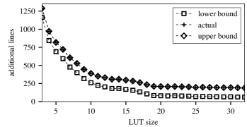
(a) Max: the actual number of additional lines often matches the upper bound; after $k=19$ increasing the LUT size has no strong effect on the number of additional lines.

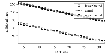
(b) Adder: the actual number of additional lines often matches the upper bound; the additional lines decrease almost linearly when increasing the LUT size.

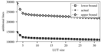
(c) Divisor: the actual number of additional lines often matches the lower bound.

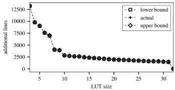
(d) Log2: the upper and lower bound are very close to each other. Note that for $k=32$ the optimum number of additional lines is achieved, since the function has 32 inputs.

Figure 5: The plots show the upper and lower bound according to Lemmas 1 and 2 as well as the actual number of additional lines when synthesizing different arithmetic benchmarks with LUT sizes ranging from 3 to 32. The $x$-axis shows LUT size and the $y$-axis shows the number of additional lines.

The lower bound inspires the following synthesis strategy that minimizes the number of additional lines. One starts by synthesizing a circuit for the output with the maximum cone. Let’s assume that this cone contains $l$ LUTs. These LUTs can be synthesized using $l$ single-target gates. Note that all of these are in fact needed, because in order to uncompute a gate, the intermediate values of children need to be available. From these $l$ gates, $l-1$ gates can be uncomputed (all except the LUT computing the output), and therefore restores $l-1$ lines which hold a constant 0 value. We can easily see that the exact number of required lines may be a bit larger, since all output values need to be kept. Note that this strategy uncomputes all LUTs in the transitive fan-in cone of an output—even if it is part of a fan-in cone of another output. Therefore, some LUTs will lead to more than two single-target gates in the reversible network.

For a good tradeoff between the number of qubits and $T$-count one is interested in the minimum number of qubits such that each LUT is translated into at most two single-target gates in the reversible network. Finding the minimum number of ancillae under such constraints relates to playing the reversible pebble game [42] in minimum time using minimum number of pebbles. More details can be found in [43, 44, 45, 46].

IV-C Synthesizing a LUT Network

Alg. 2 describes in detail how a $k$-LUT network $N=(X\cup Y\cup G,A,F)$ is mapped into a reversible network $R$ that consists of single-target gates with at most $k$ controls. The main entry point is the function ‘$\operatorname{synthesize\_mapping}$’ (line 2). This function keeps track of the current number of lines $l$, available ancillae in a stack $C$, a LUT-to-line mapping $m:G\to\mathds{N}$ that stores which LUT gates are computed on which lines in $R$, and a visited list $S$ (lines 2–2). The reference counter $r(g)$ checks for each LUT $g$ how often it is required as input to other LUTs. For driving LUTs, stored in $D$ (line 2), the reference counter is decreased by 1. It is initialized with the fan-out size and allows us to check if $g$ is not needed any longer such that it can be uncomputed (line 2). This is the case whenever the reference counter is $0$, and therefore the process of uncomputing is triggered by driving LUTs.

(a) Direct mapping.

(b) LUT-based mapping.

Figure 6: Algorithms to map a single-target gate into a Clifford+$T$ network.

Input lines are added to $R$ in lines 2–2. Input vertices are mapped to their line in $R$ using $m$. In lines 2–2 single-target gates to compute and uncompute LUTs are added to $R$. Each gate $g$ is visited in topological order (details on ‘$\operatorname{topo\_order}$’ follow later). First, a 0-initialized line $t$ is requested (line 2). Either there is one in $C$ or we get a new line by incrementing $l$. Given $t$, a single-target gate with control function $F(g)$, controls

$$m(\operatorname{fanin}(g))=\{m(g^{\prime})\mid g^{\prime}\in\operatorname{fanin}(g)\},$$ (4)

and target line $t$ is added $R$ (line 2). The LUT-to-line map is updated according to the newly added gate (line 2). Then, if $g$ is driving an output, i.e., $r(g)=0$ (line 2), we try to uncompute the children recursively by calling $\operatorname{uncompute\_children}$ (line 2). In that function, first the reference counter is decremented for each child $g^{\prime}$ that is not a primary input (line 2). Then, each child $g^{\prime}$ that afterwards has a reference count of $0$, is uncomputed using $\operatorname{uncompute\_gate}$ (line 2). In there, first it is checked whether the child has already been visited (line 2). If the child is not driving an output, a single-target gate to uncompute the line is added to $R$ (line 2). The freed line $t$ is added to $C$ (line 2) and the mapping is cleared accordingly (line 2). The child is stored as visited (line 2), and the function recurs (line 2). After all gates have been computed, outputs are added to lines in $R$ (lines 2–2). This procedure is simplified: two or more outputs may share the same driving LUT. In this case, one needs additional lines and copy the output result using a CNOT gate.

With a given topological order of LUTs, the time complexity of Alg. 2 is linear in the number of LUTs. As seen in the beginning of this section, the order in which LUTs are visited has an effect on the number of qubits. Therefore, there can be several strategies to compute a topological order on the gates. This is handled by the function ‘$\mathrm{topo\_order}$’ that is configured by a parameter in $p_{\mathrm{Q}}$. Besides the default topological order implied by the implementation of $N$ (referred to as topo_def in the following), we also implemented the order topo_tfi_sort, which is inspired by Lemma 2: compute the transitive fan-in cone for each primary output and order them by size in descending order. The topological order is obtained using a depth-first search for each cone by not including duplicates when traversing a cone.

IV-D The Role of the LUT Size

As can be seen from previous discussions, the number of additional lines roughly corresponds to the number of LUTs. Hence, we are interested in logic synthesis algorithms that minimize the number of LUTs. In classical logic synthesis the number of LUT-inputs $k$ needs to be selected according to some target architecture. For example in FPGA mapping, its value is typically 6 or 7. But for our algorithm, we can use $k$ as a parameter that trades off the number of qubits to the number of $T$ gates: If $k$ is small, one needs many LUTs to realize the function, but the small number of inputs also limits the number of control lines when mapping the single-target gates into multiple-controlled Toffoli gates. On the contrary, when $k$ is large, one needs fewer LUTs but the resulting Toffoli gates are larger and therefore require more $T$ gates. Further, since for larger $k$ the LUT functions are getting more complex, the runtime to map a single-target gate into multiple-controlled Toffoli gates increases.

To illustrate the influence of the LUT size we performed the following experiment, illustrated in Fig. 5(a). For four benchmarks and for LUT sizes $k$ from 3 to 32, we computed a LUT mapping using ABC’s [18] command ‘if -K $k$ -a’. The resulting network was used to compute both the upper and lower bound on the number of additional lines according to Lemmas 1 and 2, and to compute the actual number of lines according to Alg. 2 with ‘topo_def’ as topological order. It can be noted that the actual bound often either matches the upper bound or the lower bound. In some cases the bounds are very close to each other, leaving not much flexibility to improve on the number of additional lines. Further, after larger LUT sizes the gain in reducing the number of lines decreases when increasing the LUT size. It should be pointed out that for benchmark ‘Log2’ an optimum number of additional lines can be achieved for $k=32$, because in this case $k$ matches the number of inputs of the function. Consequently, the LUT mapping has as many gates as the number of outputs.

V Mapping Single-target Gates

For the following discussion it is important to understand the representation of the logic network that is given as input to Alg. 1 and the $k$-LUT network that from results the first step. The input network is given as a gate-level logic network, i.e., all gates are simple logic gates. In our experimental evaluation and current implementation the logic network is given as AIG, i.e., a logic network composed of AND gates and inverters. The LUT network is represented by annotating in the gate-level netlist (i) which nodes are LUT outputs and (ii) which nodes are LUT inputs for each LUT. As a result, the function of a LUT is implicitly represented as subnetwork in the gate-level logic network.

V-A Direct Mapping

The idea of direct mapping is to represent the LUT function as ESOP expression, optimize it, and then translate the optimized ESOP into a Clifford+$T$ network. Fig. 6(a) illustrates the complete direct mapping flow. As described above, a LUT function is represented in terms of a multi-level AIG. In order to obtain a 2-level ESOP expression for the LUT function, one needs to collapse the network. This process is called cover extraction and two techniques called AIG extract and BDD extract will be described in this section. The number of product terms in the resulting ESOP expression is typically far from optimal and is reduced using ESOP minimization. The optimized ESOP expression is first translated into a reversible network with multiple-controlled Toffoli gates as described in Section II-D and then each multiple-controlled Toffoli gate is mapped into a Clifford+$T$ with the mapping described in [7].

ESOP cover extraction

There are several ways to extract an ESOP expression from an AIG that represents the same function. Our implementation uses two different methods. The choice of the method has an influence on the initial ESOP expression and therefore affects both the runtime of the algorithm and the number of $T$ gates in the final network.

The method AIG extract computes an ESOP for each node in the AIG in topological order. The final ESOP can then be read from the output node. First, all primary inputs $x_{i}$ are assigned the ESOP expression $x_{i}$. The ESOP expression of an AND gate is computed by conjoining both ESOP expressions of the children, taking into consideration possible complementation. Therefore, the number of product terms for the AND gate can be as large as the product of the number of terms of the children. The final ESOP can be preoptimized by removing terms that occur twice, e.g., $x_{1}\bar{x}_{2}x_{3}\oplus x_{1}\bar{x}_{2}x_{3}=0$, or by merging terms that differ in a single literal, e.g., $x_{1}x_{3}\oplus x_{1}\bar{x}_{2}x_{3}=x_{1}x_{2}x_{3}$ [29]. AIG extract is implemented similar to the command ‘&esop’ in ABC [18]. We were able to increase the performance of our implementation by limiting the number of inputs to 32 bits, which is sufficient in our application, and by using cube hashing [47].

The method BDD extract first expresses the LUT function in terms of an AIG, again by translating each node into a BDD in topological order. From the BDD a Pseudo-Kronecker expression [48, 49] is extracted using the algorithm presented in [50]. A Pseudo-Kronecker expression is a special case of an ESOP expression. For the extracted expression, it can be shown that it is minimum in the number of product terms with respect to a chosen variable order. Therefore, it provides a good starting point for ESOP minimization. In our experiments we noticed that AIG extract was always superior and BDD extract did not show any advantage. BDD extract may be advantageous for larger LUT sizes.

ESOP minimization

In our implementation we use exorcism [29] to minimize the number of terms in the ESOP expression. Exorcism is a heuristic minimization algorithm that applies local rewriting of product terms using the EXORLINK operation [51]. In order to introduce this operation, we need to define the notation of distance. For each product term a variable can either appear as positive literal, as negative literal, or not at all. The distance of two product terms is the number of variables with different appearance in each term. For example, the two product terms $x_{1}x_{3}$ and $x_{1}\bar{x}_{2}x_{3}$ have distance 1, since $x_{2}$ does not appear in the first product term and appears as negative literal in the second one. It can be shown that two product terms with distance $k$ can be rewritten as an equivalent ESOP expression with $k$ product terms in $k!$ different ways. The EXORLINK-$k$ operation is a procedure to enumerate all $k!$ replacements for a product term pair with distance $k$. Applying the EXORLINK operation to product term pairs with a distance of less than 2 immediately leads to a reduction of the number of product terms in an ESOP expression. In fact, as described above, such checks are already applied when creating the initial cover. Applying the EXORLINK-2 operation does not increase the number of product terms but can decrease it, if product terms in the replacement can be combined with other terms. The same applies for distances larger than 2, but it can also lead to an increase in the number of product terms. This can sometimes be helpful to escape local minima. Exorcism implements a default minimization heuristic, referred to as def in the following, that applies different combinations and sequences of EXORLINK-$k$ operations for $2\leq k\leq 4$. We have modified the heuristic by just omitting the EXORLINK-4 operations, referred to as def_wo4 in the following.

Figure 7: Reversible network from Fig. 4(d). Additional lines which have a constant 0 value are drawn thicker. These lines can be used as additional resources when mapping single-target gates.

V-B LUT-based Mapping

This section describes a mapping technique that exploits two observations: (i) when mapping a single-target gate there may be additional lines available with a constant 0 value; and (ii) for single-target gates with few control lines (e.g., up to 4) one can precompute near-optimal Clifford+$T$ networks and store them in a database. Fig. 6(b) illustrates the LUT-based mapping flow. The idea is to apply 4-LUT mapping on the control function of the single-target gate and use available 0-valued lines to store intermediate results from inner LUTs in the mapping. If enough 0-values lines are available, each of the single-target gates resulting from this mapping is directly translated into a near-optimum Clifford+$T$ network that is looked up in a database. The size of the database is compressed by making use of Boolean function classification based on affine input transformations and output complementation. This procedure requires no additional lines being added to the circuit. If the procedure cannot be applied due to too few 0-valued lines, direct mapping is used as fallback.

Available 0-ancilla resources

Fig. 7 shows the same reversible network as in Fig. 4(d) that is obtained from the initial $k$-LUT mapping. However, additional lines that are 0-valued are drawn thicker. We can see that for the realization of the first single-target gate, there are three 0-valued lines, but for the last single-target gate there is only one 0-valued line. This information can easily be obtained from the reversible network resulting from Alg. 2.

The following holds in general. Let $g=\mathrm{T}_{c}(X,t)$ be a single-target gate with $|X|=k$ and let there be $l$ available 0-valued lines, besides a 0-valued line for target line $t$. If $c$ can be realized as a 4-LUT network with at most $l+1$ LUTs, then we can realize it as a reversible network with $2l-1$ single-target gates that realizes function $c$ on target line $t$ such that all inner LUTs compute and uncompute their results on the $l$ available 0-valued lines. This synthesis procedure similar but much simpler than Alg. 2, since $c$ is a single-output function. Therefore, the number of additional lines required for the inner LUTs cannot be improved by a different topological order and is solely determined by the number of LUTs in the mapping.

Near-optimal 4-input single-target gates

There exists $2^{2^{n}}$ Boolean functions over $n$ variables, i.e., $4,16,256$, and $65\,536$ for $n=1,2,3$, and $4$, respectively. Consequently, there are as many different single-target gates $\mathrm{T}_{c}(\{x_{1},\dots,x_{n}\},x_{n+1})$. For this number, it is possible to precompute optimum or near-optimal Clifford+$T$ networks for each of the single-target gates using exact or heuristic optimization methods for Clifford+$T$ gates (see, e.g., [6, 52, 53, 54]), and store them in a database. Mapping single-target gates resulting from the LUT-based mapping technique described in this sections is therefore very efficient. However, the number of functions can be reduced significantly when using affine function classification. Next, we review affine function classification and show that two optimum Clifford+$T$ networks for two single-target gates with affine equivalent functions have the same $T$-count.

For a Boolean function $f(x_{1},\dots,x_{n})$, let us use the notation $f(\vec{x})$, where $\vec{x}=(x_{1},\dots,x_{n})^{T}$. We say that two functions $f$ and $g$ are affine equivalent [55], if there exists an $n\times n$ invertible matrix $A\in\mathrm{GL}_{n}(\mathds{B})$ and a vector $\vec{b}\in\mathds{B}^{n}$ such that

$$g(\vec{x})=f(A\vec{x}+\vec{b})\qquad\text{for all $\vec{x}\in\mathds{B}^{n}$.}$$ (5)

We say that $f$ and $g$ are affine equivalent under negation [56], if either (5) holds or $g(\vec{x})=\bar{f}(A\vec{x}+\vec{b})$ for all $\vec{x}$. For the sake of brevity, we say that $f$ is AN-equivalent to $g$ in the remainder. AN-equivalence is an equivalence relation and allows to partition the set of $2^{2^{n}}$ into much smaller sets of functions. For $n=1,2,3$, and $4$, there only $2,3,6$, and $18$ classes of AN-equivalent functions (see, e.g., [56, 55, 57]. And all $4\,294\,967\,296$ 5-input Boolean functions fall into only $206$ classes of AN-equivalent functions! The database solution proposed in this mapping can therefore scale for 5 variables given a fast way to classify functions. Before we discuss classification algorithms, the following lemma shows that AN-equivalent functions preserve $T$-cost.

Lemma 3

Let $f$ and $g$ be two $n$-variable AN-equivalent functions. Then the $T$-count in Clifford+$T$ networks realizing $\mathrm{T}_{f}$ and $\mathrm{T}_{g}$ is the same.

(a) $\mathrm{T}_{f}$

(b) $\mathrm{T}_{g}$

Figure 8: A single-target gate for $\mathrm{T}_{f}$ and a single target gate for an $\mathrm{T}_{g}$, which can be constructed from $\mathrm{T}_{f}$, since $f$ and $g$ are AN-equivalent.

Proof:

Since $f$ and $g$ are AN-equivalent, there exists $A\in\mathrm{GL}_{n}(\mathds{B})$, $\vec{b}\in\mathds{B}^{n}$, and $p\in\mathds{B}$ such that $g(\vec{x})=p\oplus f(A\vec{x}+\vec{b})$ for all $\vec{x}$. It is possible to create a reversible circuit that takes $\vec{x}\mapsto A\vec{x}+\vec{b}$ using only CNOT gates for $A$ and NOT gates for $\vec{b}$ (see, e.g., [58]). The output can be inverted using a NOT gate. Fig. 8 illustrates the proof. The subcircuit $U_{A}$ realizes the linear transformation using CNOT gates, $U_{\vec{b}}$ realizes the input inversions using NOT gates, and $X^{p}$ represents a NOT gate, if $p=1$, otherwise the identity. ∎

In order to make use of the algorithm we need to compute an optimum or near-optimal circuit for one representative in each equivalence class for up to 4 variables. To match an arbitrary single-target gate with a control function of up to 4 variables in the database, one needs to derive it’s representative. Algorithms as presented in [59] can be used for this purpose.

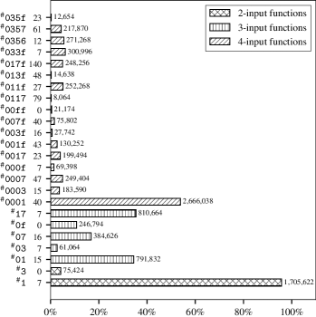
Figure 9: This plot shows the distribution of AN-equivalence classes among all 4-LUTs that have been discovered in all our experimental results (see Sect. VI). The $y$-axis shows from the bottom to the top all 2, 5, and 17 non-constant AN-equivalence classes of 2, 3, and 4 variables. The number right to the truth table is the $T$-count in the best known Clifford+$T$ realization of the corresponding single-target gate. The $x$-axis shows the frequency percentage with respect to other classes that have the same number of variables. The small number next to the bar shows the frequency in absolute values.

Fig. 9 lists all the AN-equivalent classes for 2–4 variables; the class containing the constant functions is omitted. It shows how often they are discovered in a 4-LUT in all our experimental evaluations. Also, it shows the number of $T$ gates in the best-known Clifford+$T$ networks of the corresponding single-target gate. The classes ^#1, ^#01, and ^#0001 occur most frequently. These classes contain among others $x_{1}x_{2}$, $x_{1}x_{2}x_{3}$, and $x_{1}x_{2}x_{3}x_{4}$, and are therefore control functions of the multiple-controlled Toffoli gates. The table can guide to the classes which benefit most from optimizing their $T$-count. Reversible and Clifford+$T$ networks of the best-known realizations can be found at quantumlib.stationq.com.

TABLE I: Parameters for LHRS

Parameter	Values	Description
Parameters $p_{\mathrm{Q}}$ that affect the number of qubits (and $T$ gates)
LUT size	$\{3,\dots,32\}$	Maximum number of inputs to LUTs in the LUT mapping, default: 16
Topo. order	topo_def, topo_tfi_sort	Heuristic in which order to traverse LUTs in the LUT mapping (Sect. IV-C), default: topo_def
area iters. (init)	$\{1,\dots,10\}$	Number of iterations for global area recovery heuristic based on exact area [22, 60], default: 2
flow iters. (init)	$\{1,\dots,10\}$	Number of iterations for local area recovery heursitic based on area flow [61, 62], default: 1
Parameters $p_{\mathrm{T}}$ that only affect the number of $T$ gates
Mapping	direct, hybrid	Mapping method (Sect. V), default: hybrid
ESOP extraction	AIG extract, BDD extract	ESOP extraction method (Sect. V-A), default: AIG extract
ESOP heuristic	none, def, def_wo4	ESOP minimization heuristic (Sect. V-A), none means that no optimization is applied, default: def_wo4
Parameters in hybrid mapping method
area iters.	$\{1,\dots,10\}$	see above
flow iters.	$\{1,\dots,10\}$	see above
SAT-based opt.	true, false	Enables whether 4-LUT networks in the hybrid mapping are post-optimized using the SAT-based technique described in [63], default: false

V-C Hybrid Mapping

LUT-based mapping cannot be applied if the number of available 0-valued lines is insufficient. As fallback, the 4-LUT network is omitted and direct mapping is applied on the $k$-LUT network, therefore not using any of the 0-valued lines at all. The idea of hybrid synthesis is to merge 4-LUTs into larger LUTs. By merging 2 LUTs in the network, the number of LUTs is decreased by 1 and therefore one fewer 0-valued line is required. Our algorithm for hybrid synthesis merges the output LUT with one of its children, thereby generating a larger output LUT. This procedure is repeated until the LUT network is small enough to match the number of 0-valued lines. The topmost LUT is then mapped using direct mapping, while the remaining LUTs are translated using the LUT-mapping technique.

VI Experimental Evaluation

We have implemented LHRS as command ‘lhrs’ in the open source reversible logic synthesis framework RevKit [64]. All experiments have been carried out on an Intel Xeon CPU E5-2680 v3 at 2.50 GHz with 64 GB of main memory running Linux 4.4 and gcc 5.4.

TABLE II: EPFL arithmetic benchmarks

Benchmark	Inputs	Outputs	Original		Best-LUT
			AIG nodes	Levels	LUTs	Levels
Adder	256	129	1020	255	192	64
Barrel shifter	135	128	3,336	12	512	4
Divisor	128	128	44,762	4,470	3268	1,208
Hypotenuse	256	128	214,335	24,801	40,406	4,532
Log2	32	32	32,060	444	6,574	119
Max	512	130	2,865	287	523	189
Multiplier	128	128	27,062	274	4,923	90
Sine	24	25	5,416	225	1,229	55
Square-root	128	64	24,618	5,058	3,077	1,106
Square	64	128	18,484	250	3,246	74

TABLE III: Experimental evaluation of LHRS on the EPFL arithmetic benchmarks

Bechmark	LUT size			def, direct		def_wo4, direct		def, hybrid		def_wo4, hybrid
			qubits	$T$-count	runtime	$T$-count	runtime	$T$-count	runtime	$T$-count	runtime
Adder	6	Best-LUT	448	14,411	0.13	20,487	0.11	12,623	0.18	12,721	0.18
		Original	505	6,670	0.09	6,510	0.08	2,066	0.05	2,066	0.05
	10	Best-LUT	445	18,675	0.14	24,320	0.14	13,576	0.23	13,674	0.21
		Original	490	21,357	0.15	20,313	0.14	2,860	0.05	2,860	0.04
	16	Best-LUT	443	45,577	0.68	50,946	0.37	14,699	0.29	14,797	0.28
		Original	463	313,142	20.19	309,018	19.73	5,122	0.07	5,122	0.05
Barrel shifter	6	Best-LUT	840	32,512	0.22	32,512	0.22	17,024	0.05	17,024	0.04
		Original	584	50,944	0.16	50,944	0.15	76,883	0.46	76,883	0.46
	10	Best-LUT	740	52,986	0.21	52,986	0.20	42,656	0.35	42,656	0.36
		Original	584	50,944	0.15	50,944	0.16	76,883	0.44	76,883	0.45
	16	Best-LUT	595	114,690	0.24	114,690	0.25	79,530	0.38	79,530	0.37
		Original	582	52,480	0.16	52,480	0.14	78,671	0.54	78,671	0.50
Divisor	6	Best-LUT	3,399	346,010	2.77	341,583	2.41	435,568	4.58	435,575	4.56
		Original	12,389	754,587	10.99	754,587	11.40	819,918	4.15	819,918	4.03
	10	Best-LUT	3,226	450,381	3.11	445,567	2.57	510,188	5.29	510,195	5.27
		Original	12,055	875,819	11.73	875,847	11.63	1,073,427	5.36	1,073,427	5.27
	16	Best-LUT	3,017	3,815,286	298.92	3,891,364	167.28	956,116	7.21	956,123	4.17
		Original	11,827	1,415,585	20.79	1,417,387	18.73	1,296,742	5.65	1,296,742	5.48
Hypotenuse	6	Best-LUT	40,611	3,807,147	153.97	3,672,932	152.82	5,050,507	140.24	5,050,521	140.68
		Original	47,814	2,344,226	128.06	2,314,392	126.26	3,571,061	53.98	3,571,071	65.70
	10	Best-LUT	36,443	5,902,745	166.84	5,834,737	157.12	7,893,544	153.64	7,893,427	153.90
		Original	43,871	4,345,646	123.00	4,342,966	98.62	5,430,785	74.84	5,430,737	69.24
	16	Best-LUT	32,336	20,239,832	52,944.40	20,919,129	12,382.30	11,713,691	53.25	11,716,038	48.19
		Original	39,324	22,132,834	79245.00	23,300,693	20,595.10	8,148,322	19.26	8,148,289	18.78
Log2	6	Best-LUT	6,625	664,450	5.85	660,068	4.28	1,363,770	19.69	1,363,770	19.92
		Original	7,611	501,749	4.59	501,789	3.80	996,739	3.64	996,739	3.65
	10	Best-LUT	3,038	2,036,814	45.87	2,050,844	35.18	20,342,942	49.31	20,343,371	48.84
		Original	2,875	3,284,753	70.05	3,314,383	54.05	25,548,190	47.13	25,549,307	44.61
	16	Best-LUT	2,052	56,589,962	54,824.70	59,587,462	16,412.00	44,644,140	1,661.47	44,823,085	770.26
		Original	2,315	61,071,767	94,192.60	64,461,123	27,220.50	64,368,103	1,471.36	64,447,809	448.72
Max	6	Best-LUT	1,036	56,290	0.30	55,970	0.25	19,849	0.31	19,849	0.29
		Original	1,233	71,198	0.37	69,484	0.32	64,933	0.90	64,933	0.90
	10	Best-LUT	840	195,367	1.05	193,683	0.77	25,270	0.34	25,270	0.34
		Original	901	229,669	1.05	222,761	0.70	88,221	0.88	88,221	0.84
	16	Best-LUT	725	1,082,574	57.52	1,077,303	49.81	34,488	0.40	34,400	0.39
		Original	796	748,389	36.09	745,389	30.24	94,758	1.21	94,702	1.19
Multiplier	6	Best-LUT	5,048	683,648	5.32	680,190	4.65	868,688	6.83	868,638	7.03
		Original	5,806	386,999	3.61	387,113	3.09	733,615	1.79	733,615	1.87
	10	Best-LUT	3,418	1,148,166	8.98	1,144,532	6.42	1,368,820	8.69	1,368,802	8.27
		Original	3,105	2,377,198	18.69	2,377,251	11.41	2,519,515	5.22	2,519,355	5.21
	16	Best-LUT	2,552	9,928,094	2,742.34	10,422,808	1,118.93	3,281,867	28.53	3,294,871	12.72
		Original	2,852	8,072,619	1,264.52	8,283,999	489.36	3,189,854	13.34	3,192,826	7.65
Sine	6	Best-LUT	1,277	141,885	0.72	141,456	0.64	211,143	10.36	211,143	10.13
		Original	1,468	87,624	0.76	87,872	0.60	134,664	2.24	134,664	2.29
	10	Best-LUT	557	362,108	3.55	365,175	2.39	715,314	13.20	716,079	12.67
		Original	714	408,996	3.76	411,850	2.50	1,074,871	5.45	1,074,905	5.30
	16	Best-LUT	418	3,730,177	6,579.01	3,953,575	2,210.36	1,759,815	79.38	1,791,503	44.60
		Original	518	3,820,348	1,104.20	3,913,954	390.94	3,007,519	6.86	3,008,373	6.55
Square-root	6	Best-LUT	3,204	368,301	2.76	357,593	2.42	447,805	5.39	447,798	5.40
		Original	8,212	279,275	2.95	279,275	2.97	749,687	1.35	749,687	1.35
	10	Best-LUT	2,874	549,624	4.34	542,394	3.32	566,272	7.28	566,433	7.32
		Original	7,892	323,882	3.01	323,656	3.02	833,700	1.87	833,716	1.83
	16	Best-LUT	2,632	6,158,349	392.85	6,247,981	264.42	1,404,786	16.26	1,408,346	13.51
		Original	7,816	1,524,733	948.33	1,729,343	550.70	1,028,329	1.39	1,028,401	1.34
Square	6	Best-LUT	3,309	299,986	2.54	295,325	2.28	489,565	6.92	489,617	6.85
		Original	4,058	195,290	1.54	195,312	1.78	768,725	1.98	768,725	1.35
	10	Best-LUT	2,882	532,854	2.93	531,211	2.20	826,100	7.17	826,121	7.72
		Original	3,355	464,024	2.14	464,320	1.24	1,243,876	3.38	1,243,988	2.35
	16	Best-LUT	2,303	3,964,800	26,098.40	4,142,416	7,888.93	2,303,327	8,299.69	2,355,942	2,785.77
		Original	2,664	4,249,919	29,866.40	4,470,766	7,080.61	3,075,569	8,800.60	3,156,642	1,947.58

VI-A LHRS Configuration

Table I gives an overview of all parameters that can be given as input to LHRS. The parameters are split into two groups. Parameters in the upper half have mainly an influence on the number of lines and are used to synthesize the initial reversible network that is composed of single-target gates (Sect. IV). Parameters in the lower half only influence the number of $T$ gates by changing how single-target gates are mapped into Clifford+$T$ networks. Each parameter is shown with possible values and some explanation text.

VI-B Benchmarks

We used both academic and industrial benchmarks for our evaluation. As academic benchmarks we used the 10 arithmetic instances of the EPFL combinational logic synthesis benchmarks [65], which are commonly used to evaluate logic synthesis algorithms. In order to investigate the influence of the initial logic representation, we used different realizations of the benchmarks: (i) the original benchmark description in terms of an AIG, called Original, and (ii) the best known 6-LUT network wrt. the number of lines, called Best-LUT. Further statistics about the benchmarks are given in Table II. All experimental results and synthesis outcomes for the academic benchmarks can be viewed and downloaded from quantumlib.stationq.com.

As commercial benchmarks we used Verilog netlists of several arithmetic floating point designs in half (16-bit), single (32-bit), and double (64-bit) precision. For synthesis all Verilog files were translated into AIGs and optimized for size using ABC’s ‘resyn2’ script.

TABLE IV: Experimental evaluation of LHRS on IEEE compliant floating-point designs

Benchmark				$k=6$			$k=10$			$k=16$
	size	logic depth		qubits	$T$ gates	runtime	qubits	$T$ gates	runtime	qubits	$T$ gates	runtime
add-16	788	81		230	18,351	1.03	186	24,067	1.18	156	33,521	1.35
add-32	1763	137		526	40,853	1.43	410	53,060	1.69	368	66,463	1.96
add-64	3934	252		1,194	77,843	1.74	960	109,164	2.30	867	130,990	2.41
cmp-16	110	17		65	3,720	0.16	48	7,959	0.15	40	30,426	0.77
cmp-32	202	29		126	9,261	0.20	95	16,800	0.16	81	29,335	0.21
cmp-64	374	59		245	16,519	0.23	181	34,372	0.19	163	38,967	0.25
div-16	1381	310		300	12,244	0.58	223	28,639	0.82	144	589,721	82.14
div-32	6098	1299		1,260	32,391	0.59	1,106	58,536	0.92	935	289,978	30.04
div-64	28807	5938		5,876	123,912	0.90	5,514	177,343	1.28	5,149	300,721	1.61
exp-16	4240	156		1,371	141,210	1.82	978	252,299	2.46	32	1,193,083	95,269.40
exp-32	16546	339		4,636	488,579	3.11	3,489	662,350	3.85	3,019	792,008	4.49
invsqrt-16	4017	456		899	39,410	2.03	781	119,574	3.34	32	169,282	430.99
invsqrt-32	19495	1915		4,242	118,973	3.01	4,008	349,414	4.99	3,609	703,324	6.22
invsqrt-64	97242	8830		20,874	408,652	6.21	20,274	886,327	7.89	19,536	2,009,862	10.39
ln-16	2601	86		867	139,456	3.43	303	317,543	3.92	32	1,623,461	1115.16
ln-32	11096	274		3,275	334,303	2.63	1,317	5,672,890	8.58	1,033	15,357,188	594.79
ln-64	44929	8800		13,150	254,749	4.69	12,551	370,890	5.07	12,031	1,305,192	16.52
log2-16	2592	69		937	110,827	3.04	312	317,921	3.71	32	850,331	273.23
log2-32	14102	261		4,008	436,039	2.35	1,711	8,079,605	14.81	1,244	17,600,310	496.30
log2-64	23660	3266		6,413	278,109	4.02	6,021	397,363	4.76	5,862	735,507	5.57
mult-16	1923	80		499	43,447	1.63	381	72,307	2.25	267	141,657	3.03
mult-32	5843	146		1,536	157,040	2.41	1,020	423,648	3.32	862	623,438	4.10
mult-64	21457	265		5,495	598,285	2.91	3,253	1,919,743	4.14	2,941	2,266,026	5.09
recip-16	2465	113		623	63,452	2.80	43	89,497	43.40	32	198,167	37.40
recip-32	7605	228		1,914	201,730	3.93	1,194	519,091	5.56	916	1,963,459	7.58
recip-64	42500	555		10,277	1,101,791	5.55	7,111	1,966,791	8.59	5,856	4,025,162	11.16
sincos-16	935	76		367	25,061	0.94	278	40,579	1.20	34	452,129	159.16
sincos-32	5893	201		1,740	148,104	2.25	1,438	184,706	3.14	1,284	226,328	3.46
square-16	479	39		113	12,223	0.49	35	73,381	3.20	32	133,489	6.57
square-32	2260	81		564	34,821	0.86	412	70,945	1.24	269	1,195,946	377.31
square-64	11183	166		2,788	134,370	1.25	2,251	227,490	2.04	1,803	1,054,537	176.85
sqrt-16	563	143		131	10,676	0.63	76	30,880	0.73	32	165,545	59.43
sqrt-32	2759	618		597	26,342	0.72	448	77,226	0.99	320	6,780,943	41,636.45
sqrt-64	13719	2895		2,855	80,194	0.90	2,498	222,445	1.37	2,059	3,655,540	15,194.50
sub-16	789	81		231	17,972	1.01	185	23,164	1.24	156	33,626	1.32
sub-32	1765	120		528	40,310	1.55	405	54,273	1.76	363	71,079	2.03
sub-64	3935	216		1,191	78,388	1.98	963	109,029	2.46	874	135,901	2.49

VI-C Experiments for EPFL Benchmarks

We evaluated LHRS for both realizations (Original and Best-LUT) for all 10 arithmetic benchmarks with a LUT size of 6, 10, and 16. Table III lists all results. We chose LUT size 6, because it is a typical choice for FPGA mapping, and therefore we expect that LUT mapping algorithms perform well for this size. We chose 16, since we noticed in our experiments that it is the largest LUT size for which LHRS performs reasonably fast for most of the benchmarks. LUT size 10 has been chosen, since it is roughly in between the other two. These configurations allow to synthesize 6 different initial single-target gate networks for each benchmark, therefore spanning 6 optimization points in a Pareto set. For each of these configurations, we chose 4 different configurations of parameters in $p_{\mathrm{T}}$, based on values to the mapping method and the ESOP heuristic ($\{\text{\emph{direct}},\text{\emph{hybrid}}\}\times\{\text{\emph{def}},\text{\emph{def\_wo4}}\}$).

The experiments confirm the observation of Sect. IV-D: A larger LUT size leads to a smaller number qubits. In some cases, e.g., Log2, this can be quite significant. A larger LUT size also leads to a larger $T$-count, again very considerable, e.g., for Log2.

Slightly changing the ESOP minimization heuristic (note that def to def_wo4 are very similar) has no strong influence on the number of $T$ gates. There are examples for both the case in which the $T$-count increases and in which it decreases. However, the runtime can be significantly reduced. The choice of the mapping method has a stronger influence. For example, in case of the Adder, the hybrid mapping method is far superior compared to the direct method. In many cases, the hybrid method is advantageous only for a LUT size of 16, but not for the smaller ones. Also, the initial representation of the benchmark has a considerable influence. In many cases, the Best-LUT realizations of the benchmarks require fewer qubits, which—as expected—results in higher $T$-count. The effect is particularly noticeable for the Divisor and Square-root. In some cases, better results in both qubits and $T$-count can be achieved, e.g., for Log2 as Best-LUT with a LUT size of 16, and for the Barrel shifter as Original with a LUT size of 16.

VI-D Experiments for Floating point Library

We reevaluated the LHRS algorithm in its improved implementation and new parameters on the commercial floating point designs, which were already used for the evaluation in [1]. The numbers are listed in Table IV for LUT sizes 6, 10, and 16, mapping method hybrid, and ESOP heuristic def_wo4. Due to the changes and improvements in the implementation and different parameters, the numbers vary. In the vast majority of the cases the numbers improve for qubits, $T$-count, and runtime. Consequently, we did not repeat the comparison to the hierarchical reversible logic synthesis algorithm presented in [9], as the previous numbers already have shown an improvement.

Note that for all benchmarks with 16 inputs (exp-16, invsqrt-16, ln-16, log-16, recip-16, sincos-16, square-16, and sqrt-16), a LUT size 16 leads to qubit-optimum quantum networks, since every output can be represented by a single LUT. Note that LHRS is not aware of this situation, and will realize every output separately. A better runtime, and potentially a better $T$-count, can be achieved by generating the ESOP cover and optimizing it for all outputs at once.

VI-E Compositional Functions

(a) Direct translation.

Design	qubits	$T$ gates	runtime
Direct (a)	6,355	8,960,228	manual
Resynthesis ($k=23$)	6,283	1,850,001	11.28
Resynthesis ($k=9$)	8,124	982,417	9.67

(b) Overview of results.

Figure 10: Direct implementation of the 32-bit Gaussian compared to resynthesis.

The synthesis results of the floating point benchmarks can be used to cost quantum algorithms. This alone provides a useful tool to quantum algorithm designers. However, we show below that using these results to synthesize a composed function can be sub-optimal. This is significant because several quantum algorithms require compositions of several arithmetic functions [36, 39, 66, 67, 68, 69]. We show that by using automatic synthesis with LHRS better quantum networks can be found relative to naïvely summing the costs of the constituent functions in Table IV. To demonstrate this effect, we use a 32-bit implementation of the Gaussian

$$f(x)=ae^{-\frac{(x-b)^{2}}{2c^{2}}},$$ (6)

where besides $x$ also $a,b$, and $c$ are 32-bit inputs to the quantum circuit. We focus on this function because of its importance to quantum chemistry simulation algorithms, wherein the best known simulation methods for solving electronic structure problems within a Gaussian basis need to be able to reversibly compute (6) [39]. The overheads from compiling Gaussians using conventional techniques has, in particular, rendered these simulation methods impractical. This makes improved synthesis methods critical for such applications.

The function has been used in the design of quantum algorithms. We can implement the Gaussian by combining the 32-bit versions of the floating point components (synthesized using $k=16$) in Table IV. This leads to a quantum network as shown in Fig. 10(a). Note that we use the multiplication component with a constant input to realize the denominator in the argument of the exponent. Also, we make sure to uncompute all helper lines. This leads to a quantum network with 6 355 qubits and 8 960 228 $T$ gates.

We also implemented the Gaussian directly in Verilog, optimized the resulting design with logic synthesis (as we did for the individual components in Table IV), and synthesized it using LHRS. To match the quality of the design in Fig. 10(a), we used ‘synthesize_mapping’ (see Alg. 1) to find the smallest $k$ that leads to a number of qubits smaller than 6 355. In this case, $k$ is 23. With this $k$, we synthesize the composed Guassian design using the same parameters $p_{\mathrm{T}}$ as used for synthesizing the components. The result is a quantum network with 6,283 qubits and 1,850,001 $T$ gates, which can be synthesized within 11.28 seconds (see also Fig. 10(b), which summarizes all results of this experiment).

The experiment demonstrated that by resynthesizing composed functions, better networks and better cost estimates can be achieved. The approach also easily enables design space exploration. For example, if one is interested in a quantum network with less than 1,000,000 $T$ gates, one can find a realization with 8,124 qubits and 982,417 $T$ gates, after 9.67 seconds by setting $k$ to $9$.

It can be seen that LHRS finds quantum circuits with much better qubits/$T$ gates tradeoff. Further, LHRS allows for a better selection of results by using the LUT size as a parameter. One strong advantage is that in LHRS one can quickly obtain a skeleton for the final circuit in terms of single-target gates that already has the final number of qubits. If this number matches the design constraints, one can start the computational more challenging task of finding good quantum circuits for each LUT function. Here, several synthesis passes trying different parameter configurations are possible in order to optimize the result. Also post-synthesis optimization techniques likely help to significantly reduce the number of $T$ gates.

VII Conclusion

We presented LHRS, a LUT-based approach to hierarchical reversible circuit synthesis that outperforms existing state-of-the-art hierarchical methods. It allows for much higher flexibility addressing the needs to trade-off qubits to $T$-count when generating high quality quantum networks. The benchmarks that we provide give what is at present the most complete list of costs for elementary functions for scientific computing. Apart from simply showing improvements, these benchmarks provide cost estimates that allow quantum algorithm designers to provide the first complete cost estimates for a host of quantum algorithms. This is an essential step towards the goal of understanding which quantum algorithms will be practical in the first generations of quantum computers.

LHRS can be regarded as a synthesis framework since it consists of several parts that can be optimized separately. As one example, we are currently investigating more advanced mapping strategies that map single-target gates into Clifford+$T$ networks. Also, most of the conventional synthesis approaches that are used in the LHRS flow, e.g., the mapping algorithms to derive the $k$-LUT network, are not quantum-aware, i.e., they do not explicitly optimize wrt. the quality of the resulting quantum network. We expect further improvements, particularly in the number of $T$ gates, by modifying the synthesis algorithms in that direction.

Acknowledgment

We wish to thank Matthew Amy, Olivia Di Matteo, Vadym Kliuchnikov, Giulia Meuli, and Alan Mishchenko for many useful discussions. All circuits in this paper were drawn with the qpic tool [70]. This research was supported by H2020-ERC-2014-ADG 669354 CyberCare, the Swiss National Science Foundation (200021-169084 MAJesty), and the ICT COST Action IC1405.

References

- [1] M. Soeken, M. Roetteler, N. Wiebe, and G. De Micheli, “Hierarchical reversible logic synthesis using LUTs,” in Design Automation Conference, 2017.
- [2] S. Debnath, N. M. Linke, C. Figgatt, K. A. Landsman, K. Wright, and C. Monroe, “Demonstration of a small programmable quantum computer with atomic qubits,” Nature, vol. 536, pp. 63–66, 2016.
- [3] N. M. Linke, D. Maslov, M. Roetteler, S. Debnath, C. Figgatt, K. A. Landsman, K. E. Wright, and C. Monroe, “Experimental comparison of two quantum computing architectures,” Proceedings of the National Academy of Sciences, vol. 114, no. 13, pp. 3305–3310, 2017.
- [4] E. A. Martinez, C. A. Muschik, P. Schindler, D. Nigg, A. Erhard, M. Heyl, P. Hauke, M. Dalmonte, T. Monz, P. Zoller, and R. Blatt, “Real-time dynamics of lattice gauge theories with a few-qubit quantum computer,” Nature, vol. 534, pp. 516–519, 2016.
- [5] P. J. J. O’Malley et al., “Scalable quantum simulation of molecular energies,” Physical Review X, vol. 6, p. 031007, 2016.
- [6] M. Amy, D. Maslov, M. Mosca, and M. Roetteler, “A meet-in-the-middle algorithm for fast synthesis of depth-optimal quantum circuits,” IEEE Trans. on CAD of Integrated Circuits and Systems, vol. 32, no. 6, pp. 818–830, 2013.
- [7] D. Maslov, “Advantages of using relative-phase Toffoli gates with an application to multiple control Toffoli optimization,” Physical Review A, vol. 93, p. 022311, 2016.
- [8] M. Rawski, “Application of functional decomposition in synthesis of reversible circuits,” in Int’l Conf. on Reversible Computation, 2015, pp. 285–290.
- [9] M. Soeken and A. Chattopadhyay, “Unlocking efficiency and scalability of reversible logic synthesis using conventional logic synthesis,” in Design Automation Conference, 2016, pp. 149:1–149:6.
- [10] M. Soeken, M. Roetteler, N. Wiebe, and G. De Micheli, “Design automation and design space exploration for quantum computers,” in Design, Automation and Test in Europe, 2017.
- [11] D. Große, R. Wille, G. W. Dueck, and R. Drechsler, “Exact multiple-control Toffoli network synthesis with SAT techniques,” IEEE Trans. on CAD of Integrated Circuits and Systems, vol. 28, no. 5, pp. 703–715, 2009.
- [12] D. M. Miller, D. Maslov, and G. W. Dueck, “A transformation based algorithm for reversible logic synthesis,” in Design Automation Conference, 2003, pp. 318–323.
- [13] M. Soeken, R. Wille, and R. Drechsler, “Hierarchical synthesis of reversible circuits using positive and negative Davio decomposition,” in Int’l Design and Test Symp., 2010, pp. 143–148.
- [14] C. H. Bennett, “Logical reversibility of computation,” IBM Journal of Research and Development, vol. 17, pp. 525–532, 1973.
- [15] K. Fazel, M. A. Thornton, and J. E. Rice, “ESOP-based Toffoli gate cascade generation,” in Pacific Rim Conference on Communications, Computers and Signal Processing, 2007.
- [16] D. Wecker and K. M. Svore, “LIQ: A software design architecture and domain-specific language for quantum computing,” arXiv preprint arXiv:1402.4467.
- [17] T. Häner, D. Steiger, and M. Troyer, “ProjectQ: An open source software framework for quantum computing,” arXiv preprint arXiv:1612.0809.
- [18] R. K. Brayton and A. Mishchenko, “ABC: an academic industrial-strength verification tool,” in Computer Aided Verification, 2010, pp. 24–40.
- [19] J. Cong and Y. Ding, “FlowMap: an optimal technology mapping algorithm for delay optimization in lookup-table based FPGA designs,” IEEE Trans. on CAD of Integrated Circuits and Systems, vol. 13, no. 1, pp. 1–12, 1994.
- [20] D. Chen and J. Cong, “DAOmap: a depth-optimal area optimization mapping algorithm for FPGA designs,” in Int’l Conf. on Computer-Aided Design, 2004, pp. 752–759.
- [21] A. Mishchenko, S. Cho, S. Chatterjee, and R. K. Brayton, “Combinational and sequential mapping with priority cuts,” in Int’l Conf. on Computer-Aided Design, 2007, pp. 354–361.
- [22] A. Mishchenko, S. Chatterjee, and R. K. Brayton, “Improvements to technology mapping for LUT-based FPGAs,” IEEE Trans. on CAD of Integrated Circuits and Systems, vol. 26, no. 2, pp. 240–253, 2007.
- [23] S. Ray, A. Mishchenko, N. Eén, R. K. Brayton, S. Jang, and C. Chen, “Mapping into LUT structures,” in Design, Automation and Test in Europe, 2012, pp. 1579–1584.
- [24] A. Kuehlmann, V. Paruthi, F. Krohm, and M. K. Ganai, “Robust Boolean reasoning for equivalence checking and functional property verification,” IEEE Trans. on CAD of Integrated Circuits and Systems, vol. 21, no. 12, pp. 1377–1394, 2002.
- [25] L. G. Amarù, P.-E. Gaillardon, and G. De Micheli, “Majority-inverter graph: A new paradigm for logic optimization,” IEEE Trans. on CAD of Integrated Circuits and Systems, vol. 35, no. 5, pp. 806–819, 2016.
- [26] A. De Vos and Y. Van Rentergem, “Young subgroups for reversible computers,” Advances in Mathematics of Communications, vol. 2, no. 2, pp. 183–200, 2008.
- [27] G. Bioul, M. Davio, and J.-P. Deschamps, “Minimization of ring-sum expansions of Boolean functions,” Philips Research Reports, vol. 28, pp. 17–36, 1973.
- [28] S. Stergiou, K. Daskalakis, and G. K. Papakonstantinou, “A fast and efficient heuristic ESOP minimization algorithm,” in ACM Great Lakes Symposium on VLSI, 2004, pp. 78–81.
- [29] A. Mishchenko and M. A. Perkowski, “Fast heuristic minimization of exclusive-sum-of-products,” in Reed-Muller Workshop, 2001.
- [30] M. A. Nielsen and I. L. Chuang, Quantum Computation and Quantum Information. Cambridge University Press, 2000.
- [31] D. Gosset, V. Kliuchnikov, M. Mosca, and V. Russo, “An algorithm for the -count,” Quantum Information and Computation, vol. 14, no. 15–16, pp. 1261–1276, 2014.
- [32] P. Selinger, “Quantum circuits of -depth one,” Physical Review A, vol. 87, p. 042302, 2013.
- [33] N. Abdessaied, M. Amy, M. Soeken, and R. Drechsler, “Technology mapping of reversible circuits to Clifford+ quantum circuits,” in Int’l Symp. on Multiple-Valued Logic, 2016, pp. 150–155.
- [34] A. Barenco, C. H. Bennett, R. Cleve, D. P. DiVincenzo, N. Margolus, P. Shor, T. Sleator, J. A. Smolin, and H. Weinfurter, “Elementary gates for quantum computation,” Physical Review A, vol. 52, no. 5, p. 3457, 1995.
- [35] C. Jones, “Low-overhead constructions for the fault-tolerant Toffoli gate,” Physical Review A, vol. 87, no. 2, p. 022328, 2013.
- [36] A. W. Harrow, A. Hassidim, and S. Lloyd, “Quantum algorithm for linear systems of equations,” Physical Review Letters, vol. 103, no. 15, p. 150502, 2009.
- [37] B. D. Clader, B. C. Jacobs, and C. R. Sprouse, “Preconditioned quantum linear system algorithm,” Physical Review Letters, vol. 110, no. 25, p. 250504, 2013.
- [38] N. Wiebe and M. Roetteler, “Quantum arithmetic and numerical analysis using Repeat-Until-Success circuits,” Quantum Information and Computation, vol. 16, pp. 134–178, 2016.
- [39] R. Babbush, D. W. Berry, I. D. Kivlichan, A. Y. Wei, P. J. Love, and A. Aspuru-Guzik, “Exponentially more precise quantum simulation of fermions in second quantization,” New Journal of Physics, vol. 18, no. 3, p. 033032, 2016.
- [40] T. D. Nguyen and R. Van Meter, “A resource-efficient design for a reversible floating point adder in quantum computing,” ACM Journal on Emerging Technologies in Computing Systems, vol. 11, no. 2, pp. 13:1–13:18, 2014.
- [41] H. Thapliyal, H. R. Arabnia, and A. Vinod, “Combined integer and floating point multiplication architecture (CIFM) for FPGAs and its reversible logic implementation,” arXiv preprint arXiv:cs/0610090.
- [42] C. H. Bennett, “Time/space trade-offs for reversible computation,” SIAM Journal on Computing, vol. 18, no. 4, pp. 766–776, 1989.
- [43] R. Královic, “Time and space complexity of reversible pebbling,” in Conf. on Current Trends in Theory and Practice of Informatics, 2001, pp. 292–303.
- [44] S. M. Chan, “Just a pebble game,” in Conference on Computational Complexity, 2013, pp. 133–143.
- [45] B. Komarath, J. Sarma, and S. Sawlani, “Reversible pebble game on trees,” in Int’l Conf. on Computing and Combinatorics, 2015, pp. 83–94.
- [46] A. Parent, M. Roetteler, and K. M. Svore, “Reversible circuit compilation with space constraints,” arXiv preprint arXiv:1510.00377.
- [47] B. Schmitt, A. Mishchenko, V. N. Kravets, R. K. Brayton, and A. I. Reis, “Fast-extract with cube hashing,” in Asia and South Pacific Design Automation Conference, 2017.
- [48] M. Davio, J.-P. Deschamps, and A. Thayse, Discrete and Switching Functions. McGraw-Hill, 1978.
- [49] T. Sasao, “AND-EXOR expressions and their optimization,” in Logic Synthesis and Optimization, T. Sasao, Ed. Kluwer Academic, 1993.
- [50] R. Drechsler, “Preudo-Kronecker expressions for symmetric functions,” IEEE Trans. on Computers, vol. 48, no. 9, pp. 987–990, 1999.
- [51] N. Song, “Minimization of exclusive sum of product expressions for mutliple-valued input incompletely specified functions,” Master’s thesis, Portland State University, 1992.
- [52] M. Amy, D. Maslov, and M. Mosca, “Polynomial-time -depth optimization of Clifford+ circuits via matroid partitioning,” IEEE Trans. on CAD of Integrated Circuits and Systems, vol. 33, no. 10, pp. 1476–1489, 2014.
- [53] O. D. Matteo and M. Mosca, “Parallelizing quantum circuit synthesis,” Quantum Science and Technology, vol. 1, no. 1, p. 015003, 2016.
- [54] D. M. Miller, M. Soeken, and R. Drechsler, “Mapping NCV circuits to optimized Clifford+ circuits,” in Int’l Conf. on Reversible Computation, 2014, pp. 163–175.
- [55] M. A. Harrison, “On the classification of Boolean functions by the general linear and affine groups,” Journal of the Society for Industrial and Applied Mathematics, vol. 12, no. 2, pp. 285–299, 1964.
- [56] ——, “The number of equivalence classes of Boolean functions under groups containing negation,” IEEE Trans. Electronic Computers, vol. 12, no. 5, pp. 559–561, 1963.
- [57] Y. Zhang, G. Yang, W. N. N. Hung, and J. Zhang, “Computing affine equivalence classes of Boolean functions by group isomorphism,” IEEE Trans. on Computers, vol. 65, no. 12, pp. 3606–3616, 2016.
- [58] M. Soeken, N. Abdessaied, and G. De Micheli, “Enumeration of reversible functions and its application to circuit complexity,” in Int’l Conf. on Reversible Computation, 2016, pp. 255–270.
- [59] M. Soeken, I. Kodrasi, and G. De Micheli, “Boolean function classifiction with -swaps,” in Reed-Muller Workshop, 2017.
- [60] J. Cong and Y. Ding, “On area/depth trade-off in LUT-based FPGA technology mapping,” IEEE Trans. VLSI Syst., vol. 2, no. 2, pp. 137–148, 1994.
- [61] J. Cong, C. Wu, and Y. Ding, “Cut ranking and pruning: Enabling a general and efficient FPGA mapping solution,” in Int’l Symp. on Field Programmable Gate Arrays, 1999, pp. 29–35.
- [62] V. Manohararajah, S. D. Brown, and Z. G. Vranesic, “Heuristics for area minimization in LUT-based FPGA technology mapping,” in Int’l Workshop on Logic and Synthesis, 2004.
- [63] B. Schmitt, A. Mishchenko, and R. K. Brayton, “SAT-based area recovery in technology mapping,” in Int’l Workshop on Logic and Synthesis, 2017.
- [64] M. Soeken, S. Frehse, R. Wille, and R. Drechsler, “RevKit: A toolkit for reversible circuit design,” Multiple-Valued Logic and Soft Computing, vol. 18, no. 1, pp. 55–65, 2012.
- [65] L. Amarù, P.-E. Gaillardon, and G. De Micheli, “The EPFL combinational benchmark suite,” in Int’l Workshop on Logic and Synthesis, 2015.
- [66] A. W. Childs, “On the relationship between continuous- and discrete-time quantum walk,” Communications in Mathematical Physics, vol. 294, no. 2, pp. 581–603, 2010.
- [67] C.-F. Chiang, D. Nagaj, and P. Wocjan, “Efficient circuits for quantum walks,” Quantum Information and Computation, vol. 10, no. 5 & 6, pp. 420–434, 2010.
- [68] D. W. Berry and A. W. Childs, “Black-box Hamiltonian simulation and unitary implementation,” Quantum Information and Computation, vol. 12, no. 1–2, pp. 29–62, 2012.
- [69] M. Ozols, M. Roetteler, and J. Roland, “Quantum rejection sampling,” ACM Trans. on Computation Theory, vol. 5, no. 3, pp. 11:1–11:33, 2013.
- [70] T. Draper and S. Kutin, “qpic: Creating quantum circuit diagrams in TikZ,” github.com/qpic/qpic, 2016.