Mass Formula for Light Nonstrange Mesons and Regge Trajectories in Quark Model

Abstract

We study the Regge-like spectra of light mesons in a relativized quark model. An analytical mass formula is presented for the light unflavored mesons with the help of auxiliary field method, by which a quasi-linear Regge-Chew-Frautschi plot is predicted for the orbitally excited states. We show that the trajectory slope is proportional to the inverse confining parameter $1/a$ up to a factor depending on the strong coupling $\alpha_{s}$ when the orbital quantum number $L$ is large. The result is tested against the experimental data of the spectra of the meson families $\pi/b$,$\rho/a$,$\eta/h$ and $\omega/f$ in the ($L$,$M^{2}$) planes, with the fitted parameters consistent with that in the literatures.

PACS number(s):14.40.Be,12.40.Nn, 12.39.Ki

Key Words Light-light mesons, Regge spectra, Quark model

1 Introduction

It is remarkable experimentally that most hadrons consisting of light quarks fall on straight lines known as ”Regge trajectories” [1],

$$M^{2}=(1/\alpha^{\prime})(J-\alpha_{0}).$$ (1)

This simple relation, referred to as Regge-Chew-Frautschi plot, enable us to group the hadrons with mass $M$ and the angular momentum $J$ into a series of rotational families’. The observation of linear behavior (1) in the hadron spectrum dates back to the 1970’s[2] and remains to be the subject of recent discussions as new states are discovered. In the case of light nonstrange mesons (which we shall discuss in this work) composed of unflavored quark and antiquark the slope parameter $\alpha^{\prime}$ varies only slightly from family to family (by less than $10\%$) [3, 4, 5, 6, 7], by which the linearity of trajectories are assumed. The validity of the linear Regge trajectories were addressed in the literatures, for instance, in [8, 9, 10] on the experimental ground. The correction to the linear trajectory are explored in [11, 12, 6], and recently in Ref. [7] for the light to heavy mesons systematically.

In the picture of AdS/QCD, Forkel et al[13, 14] predicted the mass relation to be of the Regge-like

$$M^{2}=4\lambda^{2}(J+1/2),$$ (2)

for the ground state of the mesons. In quark model, however, the linear behavior of the Regge trajectories remains to be understood[15, 16, 17, 18](to name a few). For further discussions on the Regge-like mesonic spectra, see Refs. [19, 20, 21, 22, 23, 24], for instance. For recent discussions, see Afonin[25, 26, 28] and Masjuan at al.[27] and references therein.

Purpose of this work is to revisit the Regge-like spectra of the light unflavored mesons in relativized quark model. With the help of auxiliary field (AF) method, an analytical mass formula is derived for the orbitally excited unflavored mesons, by which a quasi-linear Regge-Chew-Frautschi plot is predicted. We find that the trajectory slope is inversely proportional to the confining parameter $a$ up to a factor depending on the (averaged) strong coupling $\alpha_{s}$ and the orbital quantum number $L$. We also test the obtained mass formula by fitting the recent observed data of the light meson families’, $\pi/b$,$\rho/a$,$\eta/h$ and $\omega/f$ in the ($L$,$M^{2}$) planes. The best fitted values of model parameters($a=0.164GeV^{2}$, the vacuum constant $V_{0}=-343$MeV and $\alpha_{s}=0.57$) are given and in consistent with that of relativized quark models in the literatures. The limitation of the mass formula is discussed.

The $\eta/h$ trajectory is found to be distinctive (the best fit gives $a=0.226GeV^{2}$ and $V_{0}=-751$MeV), and it suggests that the members of this trajectory have the obvious $\bar{s}s$ component, for which the zero-quark-mass approximation in the model is invalid.

2 Quark model for light unflavored mesons

We use the relativized quark model with Hamiltonian given by [29, 30, 31, 32, 33], with the spin-dependent interactions suppressed for simplicity. The model Hamiltonian is

$$H=\sum_{i=1}^{2}\sqrt{\mathbf{p}^{2}+m_{i}^{2}}+V,$$ (3)

where

$$V=ar-\frac{4\alpha_{s}}{3r}+V_{0},$$ (4)

In (4), the first term is the linear confining potential, with the confining parameter $a$, the second is the color-Coulomb potential with $\alpha_{s}$ the strong coupling constant, and $V_{0}$ the vacuum constant. Here, $r=|\mathbf{x}_{1}-\mathbf{x}_{2}|$ is the relative coordinate of the quark $1$ and antiquark $2$, with the bare masses $m_{1}$ and $m_{2}$, respectively. We assume in our analysis that the two quarks are equal in mass, and make no attempt to differentiate between them. $V$ is the effective confining potential with the form of the linear plus Color-Coulomb parts. In the sector of heavy flavor this fom of the interquark potential is confirmed by Lattice QCD[34]. For the recent interquark potential in Lattice simulation, see [35], with $a=$ $\,0.155(19)$ reported.

We are mainly interested in the quantum-mechanical spectrum of the light mesons in the analytical form. To this aim, the auxiliary field (AF) method[36, 37, 38] is employed to transform the Hamiltonian into an analytically solvable one. The idea of the AF method is to apply the equality $\sqrt{B}=\min_{\lambda}\{\frac{B}{2\lambda}+\frac{\lambda}{2}\}$ (the minimization is achieved when $\lambda=\sqrt{B}$, $\lambda$ is positive) to rewrite the model Hamiltonian (3) as $H=\min_{\mu_{1,2},\nu}\left\{H(\mu_{1,2},\nu)\right\}$, where

$$\begin{array}[c]{c}H(\mu_{1,2},\nu)=\sum_{j=1}^{2}\left[\frac{\mathbf{p}^{2}+m_{j}^{2}}{2\mu_{j}}+\frac{\mu_{j}}{2}\right]+\frac{a^{2}r^{2}}{2\nu}+\frac{\nu}{2}\\ -\frac{4}{3}\frac{\alpha_{s}}{r}+V_{0},\end{array}$$ (5)

and the auxiliary fields, denoted as $\mu_{j}$($j=1,2$) and $\nu$ here, are operators in the quantum-mechanical sense. As a result, $H(\mu_{j},\nu)$ is equivalent to (3) up to the elimination of the fields $(\mu_{1},\mu_{2},\nu)$ with the help of the constraints

$$\begin{array}[c]{c}\delta_{\mu_{j}}H(\mu_{1,2},\nu)=0\Longrightarrow\mu_{j}\rightarrow\mu_{j,0}=\sqrt{\mathbf{p}_{j}^{2}+m_{j}^{2}},\\ \delta_{\nu}H(\mu_{1,2},\nu)=0\Longrightarrow\nu\rightarrow\nu_{0}=a|\mathbf{x}_{1}-\mathbf{x}_{2}|=ar.\end{array}$$ (6)

Here, the expectation average $\langle\mu_{i,0}\rangle$ ($i=1,2$) can be viewed as the dynamical mass of the quark $i$, and $\langle\nu_{i,0}\rangle$ as the static energy of the flux-tube (QCD string) linking the quark $1$ and $2$[39, 18].

Although the auxiliary fields are operators quantum-mechanically, the calculations simplify considerably if one considers them as real $c$-numbers[18]. They are to be eliminated, in the AF method, eventually through a minimization of the mass spectrum with respect to the AF’s, for which the optimal values of $\mu_{1,2}$ and $\nu$ are logically close to $\langle\mu_{i,0}\rangle$ and $\langle\nu_{i,0}\rangle$, respectively. For more details of the AF method applied to the mesons, see [40, 39, 18, 41, 42], and the references therein.

In the center of mass systems where the total momentum vanishes, the Hamiltonian (5) becomes

$$\begin{array}[c]{c}H(\mu_{1,2},\nu)=\frac{\mathbf{p}^{2}}{2\mu}+\frac{1}{2}\mu\omega^{2}r^{2}+\frac{\mu_{M}+\nu}{2}\\ -\frac{A}{2ar}+\frac{m_{1}^{2}}{2\mu_{1}}+\frac{m_{2}^{2}}{2\mu_{2}}+V_{0}\end{array}$$ (7)

in which $\mu_{M}=\mu_{1}+\mu_{2}$, $\mu=\mu_{1}\mu_{2}/\mu_{M}$ is the reduced mass of quark system, and

$$\omega=\frac{a}{\sqrt{\mu\nu}},$$ (8)

$$A=\frac{8}{3}\alpha_{s}a.$$ (9)

Since the first line of (7) is simply the harmonic oscillator Hamiltonian, one can, of course, diagonalize the Hamiltonian $H(\mu_{1,2},\nu)$ in (7) in the harmonic oscillator basis $|nLm\rangle$. As a result, the quantized energy $E_{N}(\mu_{1,2},\nu)=\langle|H(\mu_{1,2},\nu)|\rangle_{nLm}$ of the Hamiltonian (7) is

$$\begin{array}[c]{c}E_{N}(\mu_{1,2},\nu)=\omega\left(N+\frac{3}{2}\right)-\frac{A}{2\nu}\\ +\frac{\mu_{M}+\nu}{2}+\frac{m_{1}^{2}}{2\mu_{1}}+\frac{m_{2}^{2}}{2\mu_{2}}+V_{0},\end{array}$$ (10)

where $N=n+L$, with $n$ and $L$ the radial quantum number and the orbital angular momentum of the bound system, respectively. In deriving (10), we have estimated the contribution of the color-Coulomb term by its quantum average:

$$\begin{array}[c]{c}-\frac{4}{3}\left\langle\frac{\alpha_{s}}{r}\right\rangle\approx-\frac{4\alpha_{s}}{3\langle|\mathbf{x}_{1}-\mathbf{x}_{2}|\rangle}\\ =-\frac{A}{2\nu},\end{array}$$ (11)

where in the last step a simple relation $\langle|\mathbf{x}_{1}-\mathbf{x}_{2}|\rangle=\nu/a$, obtained from (6), has been used. In addition, we use the notation $\alpha_{s}$ again to stand for the expectation $\langle\alpha_{s}\rangle$ for simplicity. But one should bear in mind that $\alpha_{s}$ hereafter represents an appropriate average of the QCD running coupling which differs in implication from the same symbol in (4).

We note that we write presumably the band quantum number $N$ of the harmonic oscillator in (10) in the form $N=n+L$, rather than $N=2n+L$, considering that the superfluous symmetry enters in the Hamiltonian (5) which is absent in the original Hamiltonian (3) when the AF method applied: $r\rightarrow r^{2}$, and it may bring some unphysical degeneracy in the radially excited states that may not be there in the spectrum of the model (3). Another reason is that the ratio of the slope parameters for the radial and angular-momentum trajectories is approximately 1:1, as observed by Anisovich et al.[3] and suggested by Afonin [19, 20, 25, 26], Klempt [21] as well as Shifman et al. [22]. For the orbitally excited states with $n=0$, which we shall consider in this work, it is expected that the superfluous symmetry does not show up.

3 Mass formula and Regge trajectory

We consider only, in this work, the orbitally excited mesons for which the radial quantum number $n$ is set to be zero. To solve the model (3) with the AF method, one has to minimize the energy (10) and thereby eliminate the three auxiliary fields appearing in (10). This amounts to solving simultaneously the three constraints

$$\partial_{I}E_{N}(\mu_{1,2},\nu)=0(I=\mu_{1},\mu_{2},\nu),$$

which are explicitly

$$\frac{a_{N}\nu}{2\sqrt{(\mu\nu)^{3}}}\left(\frac{\mu_{2}}{\mu_{M}}-\frac{\mu_{1}\mu_{2}}{\mu_{M}^{2}}\right) =\frac{1}{2}-\frac{m_{1}^{2}}{2\mu_{1}^{2}},$$ (12)

$$\frac{a_{N}\nu}{2\sqrt{(\mu\nu)^{3}}}\left(\frac{\mu_{1}}{\mu_{M}}-\frac{\mu_{1}\mu_{2}}{\mu_{M}^{2}}\right) =\frac{1}{2}-\frac{m_{2}^{2}}{2\mu_{2}^{2}},$$ (13)

$$\frac{a_{N}\mu}{\sqrt{(\mu\nu)^{3}}} =1+\frac{A}{\nu^{2}},$$ (14)

where we denote $a_{N}\equiv a(L+3/2)$.

Since $m_{i}$ is same for quark and antiquark, one has, by symmetry, $\mu_{1}=\mu_{2}=2\mu$. It follows that $\mu_{i}=\mu_{M}/2$($i=1,2$), or equivalently, $\mu=\mu_{0}\equiv\mu_{M}/4$. Hence, (12) and (13) simplify

$$\frac{a_{N}\nu}{4(\mu\nu)^{3/2}}=1-\frac{4m^{2}}{\mu_{M}^{2}},.$$ (15)

By putting (15) into (14), one finds, with a little algebra

$$\mu_{M}=\frac{4a_{N}^{2}\nu}{(\nu^{2}+A)^{2}}=4\mu_{0},$$ (16)

or,

$$\mu_{1}=\mu_{2}=2\mu_{0}=\frac{2a_{N}^{2}\nu}{(\nu^{2}+A)^{2}}.$$ (17)

Having $\mu$ as a function of $\nu$ one can solve $\nu$ by rewriting the energy (10) as an energy functional of $\nu$. We assume the bare mass $m\simeq 0$ as it should be quite small at the scale of meson mass. When using (17), the energy (10) becomes,

$$E_{N}(\mu_{0},\nu)=\frac{3}{2}\nu+\frac{A}{2\nu}+\frac{2a_{N}^{2}\nu}{(\nu^{2}+A)^{2}}+V_{0},$$ (18)

which is minimized by the constraint equation (that is, $0=\delta_{\nu}E_{N}(\mu_{0},\nu)$)

$$3-\frac{A}{\nu^{2}}+\frac{4a_{N}^{2}}{(\nu^{2}+A)^{2}}-\frac{16a_{N}^{2}\nu^{2}}{(\nu^{2}+A)^{3}}=0.$$ (19)

To solve (19), we firstly consider the case $A/\nu^{2}\ll 1$. To the lowest order, $A/\nu^{2}\rightarrow 0$ yields

$$\nu^{2}=2a_{N}.$$ (20)

By making ansatz $\nu^{2}=2a_{N}+c_{A}A$ and putting it into (19), one can show

$$c_{A}=-\frac{3}{2},$$

which leads to, to the first order of $A/\nu^{2}$,

$$\nu^{2}\simeq 2a_{N}-\frac{3A}{2}.$$ (21)

Hence, the AF equations (12) through (14) can be solved by (17) as well as

$$\nu_{0}=\sqrt{2a\left(L+\frac{3}{2}-2\alpha_{s}\right)}.$$ (22)

Therefore, one finds, from (18)

$$\langle H\rangle_{N}=\left(\frac{3}{2}+\frac{1}{2c_{N}}\right)\nu_{0}+\frac{A}{2\nu_{0}}+V_{0}$$ (23)

with $\nu_{0}$ given by (22). In the case of $\mu_{1}=\mu_{2}$, one obtains a mass formula for the unflavored $\bar{q}q$ mesons,

$$M_{\bar{q}q}=\left(\frac{3}{2}+\frac{1}{2c_{N}}\right)\sqrt{2a\left(L+\frac{3}{2}-2\alpha_{s}\right)}+\frac{4a\alpha_{s}}{3\sqrt{2a\left(L+\frac{3}{2}-2\alpha_{s}\right)}}+V_{0},$$ (24)

in which

$$c_{N} =\frac{(\nu^{2}+A)^{2}}{4a_{N}^{2}}$$

$$=\left(1-\frac{2\alpha_{s}}{3(L+3/2)}\right)^{2}.$$ (25)

We note that $c_{N}\rightarrow 1$ when $L$ becomes large.

It follows, by squaring (24), that

$$\left(M_{\bar{q}q}-V_{0}\right)^{2}=2aw_{N}^{2}\left[L+\frac{3}{2}-2\alpha_{s}+\frac{4}{3}\frac{\alpha_{s}}{w_{N}}+\frac{(4\alpha_{s}/3)^{2}}{(2L+3-4\alpha_{s})w_{N}^{2}}\right],$$ (26)

where $w_{N}\equiv\left(3/2+1/(2c_{N})\right)$ tends to $2$ when $L$ is large. When one ignores the last term in the brackets in the RHS of (26), it leads to a quasi-linear from of the Regge-Chew-Frautschi plot

$$\left(M_{\bar{q}q}-V_{0}\right)^{2}=2a\left(\frac{3}{2}+\frac{1}{2c_{N}}\right)^{2}\left[L+\frac{3}{2}-\frac{5\alpha_{s}}{3}\right].$$ (27)

Here, the limit $w_{N}\rightarrow 2$ has been applied at which $c_{N}\rightarrow 1$.

We see that this quasi-linear plot is comparable to the linear Regge trajectories (1), if $V_{0}$ is small compared to the meson scale, that is, $V_{0}/M_{\bar{q}q}\ll 1$. Further, one can see that the slope parameter $\alpha^{\prime}$ of the trajectory (27) depends upon $L$ weakly,

$$\alpha^{\prime}=\frac{1}{2a}\left(\frac{3}{2}+\frac{1}{2}\left(1-\frac{2\alpha_{s}}{3(L+3/2)}\right)^{-2}\right)^{-2},$$ (28)

in which the relation (25) is used. This slope increases slowly with the quantum number $L$, and tends to $(8a)^{-1}$ when $L$ is very large: $\lim_{L\rightarrow\infty}$($\alpha^{\prime})=(8a)^{-1}$. The slope $(8a)^{-1}$ was also derived in Ref.[15] using the WKB approximation. It is to be compared to the slope $1/(2\pi a)$ predicted by the relativistic string model [43, 44, 45].

The strong coupling $\alpha_{s}$ enters also in both the slope (28) and the intercept,

$$-\alpha_{0} =\frac{3}{2}-2\alpha_{s}+\frac{4}{3}\frac{\alpha_{s}}{w_{N}}+\frac{(4\alpha_{s}/3)^{2}}{(2L+3-4\alpha_{s})w_{N}^{2}},$$ (29)

$$\simeq\frac{3}{2}-\frac{5\alpha_{s}}{3},$$ (30)

with

$$w_{N}\equiv\frac{1}{2}\left[3+\left(1-\frac{4\alpha_{s}}{3(2L+3)}\right)^{-2}\right].$$

It is remarkable that while the intercept (29) depends on the strong coupling $\alpha_{s}$ and $L$ it does not depend on the confining parameter $a$. The trajectory slope (28) is inversely proportional to $a$ when $L$ is large. We note that after the treatment of the color-Coulomb interaction using the AF method in section 2, $\alpha_{s}$ is in fact the averaged values of the strong coupling $\alpha_{s}(r)$ depending on the interquark distance $r$: $\alpha_{s}\rightarrow\langle|\alpha_{s}|\rangle_{N}$, and therefore we do not expect it to agree quantitatively with that of the values measured by QCD lattice simulations.

Although (24), or (26), is quite suited to actual test against the observed spectrum of light mesons, we shall conclude this section with discussion of the extreme situation $A/\nu^{2}\sim 1$ which may go beyond perturbative regime for solving (20) from the AF equation (19).

In the perturbative treatment from (20) to (21), we assumed $A/\nu^{2}\ll 1$, which may be violated when $L$ is small, say, $L=0$. This assumption can not be justified by only requiring $A/(2a_{N})$ to be small, which is case ( $A/(2a_{N})<0.54$) even in the worst case $L=0$ for the parameter setup of the Godfrey-Isgur(GI) model: $a=0.18GeV^{2}$, $\alpha_{s}\simeq 0.6$. At this typical setup, one can show numerically from (19) that $A/\nu^{2}$ decreases from $0.69$ to $0.13$, while in the case of (22) it drops rapidly from $2.67$ to $0.15$, as shown in Table 1 and Table 2, respectively.

One sees that the perturbative solution (22) is less stable near $L=0$ than the numerical one, and fails to satisfies $A/\nu^{2}\ll 1$. We expect, however, that this defect can be cured by the nice linearity[3] of the trajectories of light mesons, as seen in the linear fit(the solid line) shown in FIG. 1. When fitting (24) to the data, we choose the tendency of the theoretical slope in the ($L,M^{2}$) plot to agree with that of linear fitting without the first ($L=0$) states in the trajectories, that is, without the states $\rho(770)1^{--}$, $\eta(548)0^{-+}$,$\omega(782)1^{--}$, respectively. In the case of the $\pi/b$-trajectory, we retain the $L=1$ state $b_{1}(1235)1^{+-}$ since the $L=0$ state in this trajectory is actually the pion, which we exclude in this work due to its abnormally low mass.

TABLE 1. The estimate for $A/\nu^{2}$ in the case of the parameter setup of the GI model, made by the numerical solution($\nu_{0}$) to (23). The resulted trajectory parameters defined by (26) are also listed.

$L$	$0$	$1$	$2$	$3$	$4$	$5$
$A/\nu^{2}$	$0.69$	$0.37$	$0.26$	$0.19$	$0.16$	$0.13$
$\alpha^{\prime}(GeV^{-2})$	$0.86$	$0.80$	$0.77$	$0.75$	$0.74$	$0.74$
Intercept($\alpha_{0}$)	$1.12$	$0.65$	$0.58$	$0.56$	$0.55$	$0.54$

TABLE 2. The estimate for ${A/\nu}^{2}$ for the parameter setup of the GI model, made by solution (22), with the corresponding trajectory parameters listed also, defined by (26).

$L$	$0$	$1$	$2$	$3$	$4$	$5$
$A/\nu^{2}$	$2.67$	$0.62$	$0.35$	$0.24$	$0.18$	$0.15$
$\alpha^{\prime}(GeV^{-2})$	$0.86$	$0.80$	$0.77$	$0.75$	$0.74$	$0.74$
Intercept($\alpha_{0}$)	$1.12$	$0.65$	$0.58$	$0.56$	$0.55$	$0.54$

From Table 1 one sees that $A/\nu^{2}\ll 1$ is qualitatively justified when $L$ $\geq 2$. Generally, the smaller $\alpha_{s}$, the easier for this requirement to hold. In addition, the trajectory slope $\alpha^{\prime}$ increases slowly with $L$, while the intercept $\alpha_{0}$ decreases slowly when $L\geq 2$. To reduce effects due to the derivation of $\nu$ from the perturbative solution (22) at small $L$, we combine the guiding from the linear trajectory with the parameter range predicted by the relativized quark models [29, 30, 31, 32, 33] when confronting (24) with the data. Though the GI setup of the model parameters may not be the best fit in order to reproduce the trajectories of the four families’ considered, it is quite useful for the parameter searching for the best fit, as illustrated in the following section.

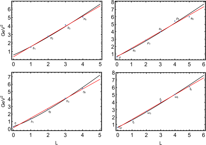
Figure 1: The linear (the solid lines) and the quasi-linear (the dashed lines) fit of the masses of the meson members in the trajectoires of the $\pi/b,\rho/a,\eta/h$ and $\omega/a$ families. The quasi-linear fit is done by the mass formula (24). The solid circles correspond to the observed data.

4 The parameters and masses

In this work, the light mesons are all assumed to be pure $\bar{q}q$ states consisting of the up or down quarks with equal mass $m\simeq 0$. To test the mass formula (24), we choose four families of light mesons, marked by $\pi/b$, $\rho/a$, $\eta/h$ and $\omega/f$, respectively. The corresponding experimental data for the family members is taken entirely from the Particle Data Group’s (PDG) 2016 Review of Particle Physics[46]. Part of the family members have been explored in Refs. [11, 3, 6], and a detailed studies were given in Refs. [17, 4, 7] associated with the Regge trajectory. The members of each trajectory has at least three states. Meanwhile, they have a feature associated with $J^{PC}$ quantum number that the orbital quantum number $L$ changes successively in trajectory, given that the pure $\bar{q}q$ state has the parity $P=(-)^{L+1}$ and $C=(-)^{L+S}$. To apply the linear-trajectory guiding mentioned in section 3 at relatively larger $L$ to the our quasi-linear fit, we list below some details of the linear fits for the trajectories selected.

(i) The $\pi/b$ trajectory($I=1$): It includes the states $b_{1}(1235)1^{+-},\pi_{2}(1670$) $2^{-+}$, $b_{3}(2030)3^{+-}$, $\pi_{4}(2250)4^{-+}$. The lowest($L=0$) state, the pion, which should have been in this trajectory, was excluded from trajectory analysis since it has abnormally low mass. The corresponding linear fit($L=1,2,3,4$), to the most recently observed data, is

$$M^{2}(\pi/b)=1.199(L+0.314),\chi_{MS}^{2}=0.0205$$

with the mean squared (MS) error $\chi_{MS}^{2}$ for the fit added. The fit is depicted in the FIG. 1(a)(the solid line), including the experimental data (the solid circles) for comparison. Here, the MS error is defined by $\chi_{MS}^{2}=\sum_{L}(M_{L}^{Th}-M_{L}^{Exp})^{2}/(L_{\max}-1)$ where the index $L$ runs from $0(1$ for the $\pi/b$ trajectory$)$ to the maximal value $L_{\max}$ of the orbital number.

(ii) The $\rho/a$ trajectory($I=1$): The members chosen are the states $\rho(770)1^{--}$, $a_{2}(1320)2^{++}$,$\rho_{3}(1690)3^{--}$, $a_{4}(2040)4^{++}$, $\rho_{5}(2350)5^{--}$ and $a_{6}(2450$) $6^{++}$. The linear fit ($L=0,1,2,3,4,5$) and its MS error are

$$M^{2}(\rho/a)=1.120(L+\allowbreak 0.565),\chi_{MS}^{2}=0.0387$$

The results of the fit is shown in the FIG. 1(b)(the solid line), compared to the data(the solid circles). In the following the same mark convention will be used when plotting the trajectories of the $\eta/h$ and $\omega/f$).

(iii) The $\eta/h$ trajectory($I=0$): The members are the states $\eta(548)0^{-+}$, $h_{1}(1170)1^{+-}$,$\eta_{2}(1645)2^{-+}$, $h_{3}(2025)3^{+-}$ and $\eta_{4}(2330)4^{-+}$. The result of the linear fit ($L=0,1,2,3,4$) is

$$M^{2}(\eta/h)=1.297(L+0.128),\chi_{MS}^{2}=0.0181$$

and depicted in the FIG. 2 (c)(the solid line).

(iv) The $\omega/f$ trajectory($I=0$): It is composed of the state members $\omega(782)1^{--}$, $f_{2}(1270)2^{++}$, $\omega_{3}(1670)3^{--}$, $f_{4}(2050)4^{++}$, $\omega_{5}(2250)5^{--}$ and $f_{6}(2510)6^{++}$. The linear fit ($L=0,1,2,3,4,5$) gives

$$M^{2}(\omega/f)=1.115(L+0.527),\chi_{MS}^{2}=0.0081$$

and is depicted in the FIG. 2 (d)(the solid line).

One sees that in its nätive form the linear formula (2) applies for the $\rho/a$ and $\omega/f$ trajectories for which $-\alpha_{0}\simeq 0.5$, but fails somehow in the case of the $\pi/b$ and $\eta/h$ trajectories for which $-\alpha_{0}\simeq 0.3$ and $0.1$, respectively.

We use (24), with $c_{N}$ given by (25), to fit the above four meson families in the ($L$, $M^{2}$) plane (we set $n=0$). The optimal parameters ($a,\alpha_{s}$,$V_{0}$) fitted to the data are shown in Table 2, in which the notation Num. stands for the number of the data coordinates. In Table 3, we show the mass values calculated from the mass formula (24) and masses of the experiment (PDG) [46], with the corresponding MS error $\chi_{MS}^{2}$ listed also.

TABLE 3. The optimal values for the confining parameter($a$), the strong coupling($\alpha_{s}$) averaged and the vacuum constant $V_{0}$ for fitting (24) to the experimental (PDG) mass data[46]. The calculated trajectory parameters, when $L=4$(for $\pi/b,\eta/h$) and $L=5$(for $\rho/a,\omega/f$), and the MS error $\chi_{MS}^{2}$ for fitting are also listed.

Traj.	Num.	$a$(GeV2)	$\alpha_{s}$	$V_{0}$(GeV)	$\chi_{MS}^{2}$(GeV)
$\pi/b$	$4$	$0.165$	$0.584$	$-0.351$	$0.00299$
$\rho/a$	$6$	$0.167$	$0.562$	$-0.360$	$0.00255$
$\eta/h$	$5$	$0.226$	$0.581$	$-0.751$	$0.00335$
$\omega/f$	$6$	$0.159$	$0.562$	$-0.325$	$0.00176$

        

It can been seen from Table 3 that the optimal values of the model parameters (confining parameter $a$, strong coupling $\alpha_{s}$, vacuum constant $V_{0}$) fall in the regime around the GI setup, except for the $\eta/h$ trajectory for which $a$ and $-V_{0}$ are obviously larger. One can explain this exceptional case as an indication that the members of $\eta/h$ trajectory may have hidden $\bar{s}s$ component, which goes beyond the approximation $m\simeq 0$ taken in this work. When the $\eta/h$ trajectory removed, the fitted values of $a,\alpha_{s}$ and $V_{0}$ vary slightly at the level of $1.5\%$, $2.3\%$ and $9\%$ respectively. In this sense, we conclude that three model parameters $a,\alpha_{s}$ and $V_{0}$ are universal, and has a globally fit at about

$$a=0.164\text{GeV}^{2}\text{,}V_{0}=-343\text{MeV, }\alpha_{s}=0.57\text{.}$$ (31)

The trajectory slope at the global fit is

$$\alpha^{\prime}=0.871(6)\text{GeV}^{-2}\text{.}$$ (32)

For the intercept, no universal fit can be found. The above prediction for $\alpha^{\prime}$ is in good agreement with that of the models in the literatures, say, $0.886GeV^{2}$ in Ref.[11], $0.887GeV^{2}$ in Ref.[17](for the $\rho$ parent trajectory), $0.884$ in Ref.[7], and $0.893$($=1/1.12$) in Ref.[4].

On the other hand, the study[47] of the parameters of the relativized quark model provides a constraint on them: $200$MeV$\leq-V_{0}\leq 470$MeV. This constraints are fulfilled by all fitted parameters in Table 3, except for the $\eta/h$ trajectory. Given that $\alpha_{s}$ is the averaged value of the strong coupling in (3) the fit (31) agrees well with the parameter setup of the GI model[32](where $\alpha_{s}\leq 0.60$). For the parameter $a$, the fit in (31) is compatible with the results of the literatures:$a=0.180$ in Ref.[31];$a=0.192$ in Ref.[33];$a=0.191$ in Ref.[48];$a=0.183$ in Ref.[49]. We stress here that our fit for $a$ in (31) is closer to the confining parameter $\sigma$ in the recent lattice simulation[35]: $(0.394(17))^{2}\simeq 0.155(19)$.

TABLE 4. The calculated masses(MeV) and that of the experiment (PDG) [46] for the four light meson families. The states marked with solid triangles are the established states given in the PDG summary tables, while those marked an ‘f.’ are the less established mesons given in further states. The notation ”Num.” stands for the numerical prediction by solving the model (24).

Traj.	$\begin{array}[c]{r}\text{{\ mesons }}}{\\ \text{(}J^{PC}\text{ {\small Status})}\end{array}$	Exp.	This work	Num.	$\par\begin{array}[c]{r}\text{{\small Calculations in Refs.\ }}\\ \text{{\small GI\cite[cite]{[\@@bibref{}{GodfreyIsgur:85}{}{}]},EF\cite[cite]{[\@@bibref{}{EbertFG:D09}{}{}]},SW\cite[cite]{[\@@bibref{}{SonnenscheinW:JHEP14}{}{}]}}}\end{array}$
$\begin{array}[c]{r}\pi/b\\ (I=1)\end{array}$	$\begin{array}[c]{rrr}b_{1}&1^{+-}&\blacktriangle\\ \pi_{2}&2^{-+}&\blacktriangle\\ b_{3}&3^{+-}&\text{f }\\ \pi_{4}&4^{-+}&\text{f }\end{array}$	$\begin{array}[c]{r}1229\\ 1672\\ 2030\\ 2250\end{array}$	$\begin{array}[c]{r}1302\\ 1666\\ 1972\\ 2242\end{array}$	$\begin{array}[c]{r}1241\\ 1631\\ 1951\\ 2230\end{array}$	$\begin{array}[c]{rrr}1220&1258&1257\\ 1680&1643&1650\\ 2030&2164&1965\\ 2330&2344&2236\end{array}$
$\begin{array}[c]{r}\rho/a\\ (I=1)\end{array}$	$\begin{array}[c]{rrr}\rho&1^{--}&\blacktriangle\\ a_{2}&2^{++}&\blacktriangle\\ \rho_{3}&3^{--}&\blacktriangle\\ a_{4}&4^{++}&\blacktriangle\\ \rho_{5}&5^{--}&\\ a_{6}&6^{++}&\end{array}$	$\begin{array}[c]{r}775\\ 1318\\ 1689\\ 1995\\ 2330\\ 2450\end{array}$	$\begin{array}[c]{r}839\\ 1310\\ 1675\\ 1982\\ 2253\\ 2497\end{array}$	$\begin{array}[c]{r}678.5\\ 1243\\ 1634\\ 1956\\ 2236\\ 2487\end{array}$	$\begin{array}[c]{rrr}770&776&776\\ 1310&1317&1324\\ 1680&1714&1701\\ 2010&2018&2008\\ 2300&2264&2274\\ &2475&2511\end{array}$
$\begin{array}[c]{r}\eta/h\\ (I=0)\end{array}$	$\begin{array}[c]{rrr}\eta&0^{-+}&\blacktriangle\\ h_{1}&1^{+-}&\blacktriangle\\ \eta_{2}&2^{-+}&\blacktriangle\\ h_{3}&3^{+-}&\text{f }\\ \eta_{4}&4^{-+}&\text{f }\end{array}$	$\begin{array}[c]{r}548\\ 1170\\ 1617\\ 2025\\ 2328\end{array}$	$\begin{array}[c]{r}638\\ 1185\\ 1611\\ 1969\\ 2285\end{array}$	$\begin{array}[c]{r}462.6\\ 1124\\ 1581\\ 1955\\ 2282\end{array}$	$\begin{array}[c]{rrr}520&&545\\ 1220&1485&1206\\ 1680&1909&1612\\ 2030&2209&1933\\ 2330&2806&2208\end{array}$
$\begin{array}[c]{r}\omega/f\\ (I=0)\end{array}$	$\begin{array}[c]{rrr}\omega&1^{--}&\blacktriangle\\ f_{2}&2^{++}&\blacktriangle\\ \omega_{3}&3^{--}&\blacktriangle\\ f_{4}&4^{++}&\blacktriangle\\ \omega_{5}&5^{--}&\text{f }\\ f_{6}&6^{++}&\text{f }\end{array}$	$\begin{array}[c]{r}783\\ 1275\\ 1667\\ 2018\\ 2250\\ 2469\end{array}$	$\begin{array}[c]{r}846\\ 1305\\ 1661\\ 1961\\ 2225\\ 2464\end{array}$	$\begin{array}[c]{r}695.4\\ 1247\\ 1628\\ 1942\\ 2215\\ 2461\end{array}$	$\begin{array}[c]{rrr}780&&768\\ 1280&1529&1319\\ 1680&1950&1698\\ 2010&2286&2006\\ 2300&2559&2271\\ &2465&2509\end{array}$

From Tables 4 we observe that the calculated masses from (24) are systematically larger than the experimental values as well as that of the references cited in the case of the low-$L$ states($L=0,1$). The ratio between the prediction in this work and the experiment is about $1.04-1.14$ for the ($L=1$) states $b_{1}(1235)1^{+-}$ and the ($L=0$) states,$\rho(770)1^{--}$, $\eta(548)0^{-+}$, $\omega(782)1^{--}$. This should not be surprise considering that the perturbative solution (22) fails to satisfy $A/\nu^{2}\ll 1$ near $L=0$ and $1$, as seen from Table 1. This entails the nonperturbatively solving of the AF equation (19) for the static energy $\nu$ of string. One simple and direct way to do this is, for instance, to promote (22) into an ansatz $\nu_{0}^{2}=2a\left(L+\frac{3}{2}-f(\alpha_{s})\right)$ and solve the unknown function $f(\alpha_{s})$ numerically or analytically (such a work is under way).

One of other limitations of the mass formula (24) comes from the chiral limt (zero-mass limit) approximation for the light quark. This approximation fails when meson has mixed hidden $\bar{s}s$(or $\bar{c}c$) component in its internal structure. In this case, the calculation by the mixed state $|\bar{q}q\rangle+|\bar{s}s\rangle$ is needed, for which the strange quark mass $m_{s}$ is expected to enter in the mass formula (24). Another limitation comes from the two-quark state ($\bar{q}q$) assumption for mesons. This assumption may not be true when a meson has exotic structure, such as components of gluoballs and/or multiquark states. This goes beyond the picture of the native quark model used in this work and may make the mass formula (24) insufficient.

5 Summary

We re-visit the orbital Regge spectra of the light unflavored mesons in the framework of relativized quark model. By applying the auxiliary field method to model, an analytical mass formula is proposed for the orbitally excited unflavored mesons, by which a quasi-linear Regge-Chew-Frautschi plot is predicted. We test the mass formula by fitting the observed data of the light meson families’, $\pi/b$,$\rho/a$,$\eta/h$ and $\omega/f$ in the ($L$,$M^{2}$) planes, and find that the optimal values of the model parameters are consistent with that of the relativized quark models in the literatures. An agreement of the mass predicted by the mass formula with the experimental data is achieved for the meson families considered.

It is also shown for large orbital quantum number $L$ that the trajectory slope is inversely proportional to the confining parameter $a$, while the intercept depends on the strong coupling $\alpha_{s}$, independent of $a$.

The anomaly is observed in the fitted parameters when comforting the mass formula with the experimental spectra of the $\eta/h$ trajectory. This may imply that the unflavored states $\eta(548)0^{-+}$, $h_{1}(1170)1^{+-}$ and others in the $\eta/h$ trajectory either have mixed with hidden $\bar{s}s$(or $\bar{c}c$) component in its internal structure or go beyond the two-quark picture.

Acknoledgements

D. J thanks X. Liu for useful discussions. D. J is supported by the National Natural Science Foundation of China under the no. 11565023 and the Feitian Distinguished Professor Program of Gansu(2014-2016). C-Q. P is supported by the High-End Creative Talent Thousand People Plan of Qinghai Province, No. 0042801 and the Applied Basic Research Project of Qinghai Province, No. 2017-ZJ-748. A.H is supported by Grants-in-Aid for Scientific Research (Grants No. JP26400273(C) and JP25247036(A)).

References

- [1] G. F. Chew, and S. C. Frautschi, Phys. Rev. Lett. 7,394 (1961).
- [2] P. Collins, An Introduction to Regge Theory and High Energy Physics, (Cambridge Univ. Press, Cambridge,1977,456).
- [3] A. Anisovich, V. Anisovich, and A. Sarantsev, Phys.Rev. D 62,051502 (2000);[hep-ph/0003113].
- [4] Pere Masjuan,E. R. Arriola and W. Broniowski, Phys.Rev. D 85, 094006 (2012).
- [5] G. Sharov, String Models, Stability and Regge Trajectories for Hadron States, arXiv:1305.3985.
- [6] A. Selem and F. Wilczek, Hadron systematics and emergent diquarks, [hep-ph/0602128].
- [7] J. Sonnenschein and D. Weissman, JHEP 1408,013 (2014); [arXiv:1402.5603].
- [8] A. Inopin, and G. S. Sharov, Phys. Rev. D 63 ,054023 (2001).
- [9] A. Tang and J. W. Norbury, Phys.Rev. D 62 , 016006 (2000); [hep-ph/0004078].
- [10] Xin-Heng Guo, Ke-Wei Wei, X. H. Wu, Phys.Rev. D 78, 056005 (2008).
- [11] K. Johnson and C. Nohl, Phys.Rev. D 79, 291 (1979).
- [12] M.M. Brisudova, L. Burakovsky and T. Goldman, Phys.Rev. D 61, 054013 (2000).
- [13] H. Forkel, M. Beyer, and T. Frederico, Int. J. Mod. Phys. E 16, 2794 (2007).
- [14] H. Forkel, M. Beyer, and T. Frederico, JHEP 07,077 (2007).
- [15] J. S. Kang and H. J. Schnitzer, Phys. Rev. D 12,841 (1975).
- [16] K. M. Maung, D. E. Kahana and J. W. Norbury,Phys. Rev. D 47, 1182 (1993).
- [17] D. Ebert, R. Faustov, and V. Galkin, Phys. Rev. D 79,114029 (2009); [arXiv:0903.5183].
- [18] B. Silvestre-Brac, C. Semay and F. Buisseret, J. Phys. A 41, 425301 (2008).
- [19] S. S. Afonin, Mod. Phys. Lett. A 22, 1359 (2007).
- [20] S. S. Afonin, Phys.Rev. C 76, 015202 (2007).
- [21] E. Klempt and A. Zaitsev, Phys. Rep 454, 1 (2007).
- [22] M. Shifman and A. Vainshtein, Phys. Rev. D 77, 034002(2008).
- [23] S. S. Afonin, Int. J. Mod. Phys. A 22, 4537 (2007).
- [24] S. S. Afonin, Int. J. Mod. Phys. A 23, 4205 (2008).
- [25] S. S. Afonin and I. V. Pusenkov, Phys. Rev. D 90, 094020 (2014).
- [26] S. S. Afonin and I. V. Pusenkov, Mod. Phys. Lett. A 29, 1450193 (2014).
- [27] P. Masjuan, E. R. Arriola and W. Broniowski, EPJ Web Conf. 73, 04021 (2014).
- [28] S. S. Afonin, Acta Phys.Polon.Supp. 9, 597(2016).
- [29] B. Durand and L. Durand, Phys. Rev. D 25, 2312 (1982).
- [30] D. B. Lichtenberg, W. Namgung, E. Predazzi, and J. G. Wills, Phys. Rev. Lett. 48, 1653 (1982).
- [31] B. Durand and L. Durand, Phys. Rev. D 30, 1904 (1984).
- [32] S. Godfrey and N. Isgur, Phys. Rev. D 32,189 (1985).
- [33] S. Jacobs, M. G. Olsson, and C. J. Suchyta III, Phys. Rev. D 33, 3338 (1986)
- [34] G.S. Bali, Phys. Rept. 343, 1 (2001).
- [35] T. Kawanai and S. Sasaki, Prog. Part. Nucl. Phys. 67, 130 (2012).
- [36] A.M. Polyakov, Gauge Fields and Strings, (Harwood Academic Publishers,Poststrasse,1987).
- [37] E. L. Gubankova and A. Yu. Dubin, Phys. Lett. B 334, 180 (1994); [hep-ph/9408278].
- [38] L. Morgunov, A. V. Nefediev and Yu. A. Simonov, Phys. Lett. B 459, 653 (1999).
- [39] C. Semay, B. Silvestre-Brac and I. M. Narodetskii,Phys. Rev. D 69,014003 (2004).
- [40] Yu.S. Kalashnikova, A.V. Nefediev, Phys. Lett. B 492, 91 (2000).
- [41] Yu. A. Simonov, Phys. Lett. 226, 151 (1988).
- [42] 42. Yu. S. Kalashnikova and A. V. Nefediev, Phys. At. Nucl. 60, 1389 (1997).
- [43] T. Goto, Prog. Theor. Phys. 46,1560 (1971).
- [44] P. Goddard, J. Goldstone, C. Rebbi, C.B. Thorn, Nucl.Phys. B 56,109 (1973).
- [45] Y. Nambu, Phys. Rev. D 10, 4262 (1974).
- [46] C. Patrignani et al. (Particle Data Group),Chin.Phys. C 40, 100001 (2016).
- [47] S. Veseli and M. G. Olsson, Phys.Lett. B 383, 109 (1996).
- [48] L. P. Fulcher, Z. Chen and K. C. Yeong, Phys. Rev. D 47,4122 (1993).
- [49] D. S. Hwang and G.-H. Kim, Phys. Rev. D 53, 3659 (1996).