A new temperature dependent hyperonic equation of state: application to rotating neutron star models and $I$-$Q$-relations.

Abstract

In this work we present a newly constructed equation of state (EoS) –applicable to stellar core collapse and neutron star mergers–, including the entire baryon octet. Our EoS is compatible with the main constraints from nuclear physics and, in particular, with a maximum mass for cold $\beta$-equilibrated neutron stars of $2M_{\odot}$ in agreement with recent observations. As an application of our new EoS, we compute numerical stationary models for rapidly (rigidly) rotating hot neutron stars. We consider maximum masses of hot stars, such as proto-neutron stars or hypermassive neutron stars in the post-merger phase of binary neutron star coalescence. The universality of $I$-$Q$-relations at nonzero temperature for fast rotating models, comparing a purely nuclear EoS with its counterparts containing $\Lambda$-hyperons or the entire baryon octet, respectively, is discussed, too. We find that the $I$-$Q$ universality is broken in our models when thermal effects become important, independent on the presence of entropy gradients. Thus, the use of $I$-$Q$ relations for the analysis of proto neutron stars or merger remnant data, including gravitational wave signals from the last stages of binary neutron star mergers, should be regarded with care.

I Introduction

Neutron stars are among the most extreme objects in the universe. They represent unique laboratories for probing strongly interacting matter at ultra high densities –exceeding that in atomic nuclei–, as well as gravity for strong fields. They are formed in a core-collapse supernovae (CCSN) and cool down mainly by neutrino emission to form a catalyzed cold neutron star on a timescale of several minutes. Thus, in the early post bounce phase, as proto-neutron stars (PNS), they do not contain only ultra-dense matter, but they are hot objects, too, reaching temperatures of the order $\sim 50$ MeV Burrows and Lattimer (1986); Keil and Janka (1995); Pons et al. (1999). In addition, matter in a PNS is not transparent to neutrinos, being thus lepton rich. Temperature and lepton content are important ingredients to describe the physics of PNSs, be it matter composition and stability of the PNS against collapse to a black hole Keil and Janka (1995); Baumgarte et al. (1996); Pons et al. (2001); Ishizuka et al. (2008); Sumiyoshi et al. (2009); Nakazato et al. (2010, 2012); Hempel et al. (2012); Peres et al. (2013); Steiner et al. (2013); Char et al. (2015) or dynamical properties such as frequencies and damping times of quasi-normal modes and consequently the emitted gravitational wave signal Ferrari et al. (2003).

In the post-merger phase of a binary neutron star coalescence, a rapidly rotating neutron star could be formed which temporarily resists to a black hole collapse Sekiguchi et al. (2011), even if its mass exceeds the maximum mass of a cold non-rotating neutron star. Within these merger remnants, temperatures of the same order as for CCSN and PNSs are reached. Both, PNSs and merger remnants can rotate at rather high frequencies, with potentially a differential rotation profile.

The temperatures of 50-100 MeV, reached in these astrophysical environments are such that thermal effects on the EoS become important. They have in particular a non-negligible effect on the composition, favoring the production of non-nucleonic degrees of freedom such as hyperons, nuclear resonances, or mesons. Even a transition to the quark-gluon plasma could take place. The impact of these additional particles on the evolution of PNSs has a long history, see e.g. Prakash et al. (1997) for an early review. Most models employ EoS for homogeneous matter, neglecting inhomogeneous matter in the outer layers and the formation of a crust, see e.g. Pons et al. (2001, 2000); Nicotra et al. (2006); Menezes and Providencia (2007); Dexheimer and Schramm (2008); Yasutake and Kashiwa (2009); Bombaci et al. (2007); Burgio et al. (2011); Chen et al. (2012).

Currently, only a few EoSs are available covering in a consistent way the whole necessary domain in temperature $T$, baryon number density $n_{B}$ and electron fraction, $Y_{e}=n_{e}/n_{B}$ where $n_{e}$ is the electron number density. We will call them general purpose EoS. In the last years, a series of new EoS models has been developed, see e.g. Botvina and Mishustin (2010); Typel et al. (2010); Hempel and Schaffner-Bielich (2010); Shen et al. (2011a, b); Raduta and Gulminelli (2010); Steiner et al. (2013); Hempel et al. (2012); Furusawa et al. (2013); Togashi et al. (2017); Furusawa et al. (2017), focused mainly on the treatment of the inhomogeneous part and correct nuclear abundances, and/or nuclear interactions at high densities. Triggered by investigations of stellar black hole formation, some effort has recently been devoted to extend the existing purely nuclear models to include non-nucleonic degrees of freedom –hyperons, pions or quarks– at high densities and temperatures, too, see e.g. Ishizuka et al. (2008); Nakazato et al. (2008); Sagert et al. (2009); Shen et al. (2011); Oertel et al. (2012); Gulminelli et al. (2013); Banik et al. (2014). The latter are very important for the description of PNSs and merger remnants in view of the high densities combined with high temperatures which are attained within these objects. However, up to now none of these extended models is really satisfactory, since either not compatible with constraints from nuclear physics or neutron star masses Demorest et al. (2010); Antoniadis et al. (2013); Fonseca et al. (2016), or containing only a limited selection of additional degrees of freedom, typically $\Lambda$-hyperons. Here, we will present for the first time an EoS taking into account the entire baryon octet and being well compatible with the main present constraints.

As an application of our new EoS, we will compute stationary models of (rotating) hot stars and study the influence of hyperons on PNS and merger remnant properties. Most studies of PNS evolution are based on sequences of quasi-equilibrium models, an assumption which is well justified in view of the hydrodynamic timescale ($\lesssim 10^{-3}$ s) being much smaller than the timescale on which thermodynamic properties are modified considerably ($\approx 1$ s), see e.g. Burrows and Lattimer (1986); Pons et al. (2001); Villain et al. (2004). Although merger remnants cannot be well approximated as being in a quasi-equilibrium state, interest in stationary models of these stars arise in order to understand the physical mechanism stabilizing the hypermassive star without performing a complete numerical merger simulation.

Stationary models of (cold) relativistic stars have been extensively explored in the literature. The first models, the famous Tolman-Oppenheimer-Volkoff solutions, describing spherically symmetric (therefore non-rotating) stars, date from the late 1930’s Tolman (1939); Oppenheimer and Volkoff (1939). Hartle and Thorne proposed the first axisymmetric rotating solutions from a perturbative approach in the slow rotation approximation Hartle and Thorne (1968). Nowadays several publicly available codes are able to obtain precise numerical solutions up to the mass shedding limit Nozawa et al. (1998); Ansorg et al. (2009), at the Kepler frequency, see e.g. the textbook by Friedman and Stergioulas (2013). However, all these solutions only treat cold $\beta$-equilibrated stars with a barotropic EoS. Goussard et al. Goussard et al. (1998, 1997) have introduced the first models including the effect of finite temperature, restricting their solution however to the isentropic or isothermal case in $\beta$-equilibrium with several fixed overall lepton fractions, where the EoS effectively reduces to a barotropic one. Refs. Martinon et al. (2014); Camelio et al. (2016) propose general solutions within a perturbative slow rotation approach. In this work, we follow Ref. Villain et al. (2004) to consistently compute stationary rapidly rotating hot stars based on the publicly available numerical library lorene Gourgoulhon et al. (2016).

The paper is organized as follows. In Sec. II we present the new EoS model and in Sec. III some of its properties and in particular its compatibility with available constraints. In Sec. IV we present the formalism to treat stationary rotating relativistic stars at nonzero temperature. Sec. V shows first applications of our models, discussing maximum masses of hot stars and $I$-$Q$ relations, i.e., universal relations among the moment of inertia and the quadrupole moment. We conclude in Sec. VI. Throughout the paper we use natural units with $c=\hbar=k_{B}=1$ where appropriate.

II Equation of state

Although the transition to the quark-gluon plasma is very interesting, as it could facilitate the supernova explosion Sagert et al. (2009), explain some gamma-ray bursts Pili et al. (2016), or – within the scenario of “quark-novae” – some unusual supernova lightcurves Ouyed et al. (2002, 2013); Buballa et al. (2014), we will concentrate here on hyperonic degrees of freedom. Presently available general purpose EoS models including all hyperons and covering the entire range in baryon number density, $n_{B}$, temperature $T$ and hadronic charge fraction, $Y_{Q}=n_{Q}/n_{B}=Y_{e}$  necessary for applications in CCSN or binary mergers, are either not compatible with some constraints from nuclear physics and/or a neutron star maximum mass of $2M_{\odot}$, see e.g. Ishizuka et al. (2008); Oertel et al. (2012) or consider only $\Lambda$-hyperons (e.g. Banik et al. (2014)). Our new EoS, taking into account the entire baryon octet, is well compatible with the main present constraints, see Sec. III for details.

II.1 Statistical model for inhomogeneous matter

At subsaturation densities and low temperatures, nucleonic matter is unstable with respect to variations in the particle densities and becomes inhomogeneous, i.e. nuclei or more generally nuclear clusters are formed. The critical temperature is of the order $\sim 15$ MeV just below saturation and decreases to about 1 MeV at lower densities. Below a density of roughly $n_{B}\sim 10^{-4}\mathrm{fm}^{-3}$, the cluster size is very small compared with its mean free path, such that matter can be described as a non-interacting gas of nuclei, nucleons and leptons in thermodynamic equilibrium. This approach is generally called “nuclear statistical equilibrium” (NSE). In the last years several models have been developed to go beyond a pure NSE and take into account nucleon interactions and the interaction of clusters with the surrounding medium at higher densities (see e.g. Raduta and Gulminelli (2010); Gulminelli and Raduta (2015); Hempel and Schaffner-Bielich (2010); Typel et al. (2010); Sumiyoshi and Röpke (2008); Buyukcizmeci et al. (2014); Heckel et al. (2009)). In stellar matter particular attention has to be paid to the interplay between the short-range nuclear interaction and the long-range Coulomb interaction, which determines sizes and shapes of the nuclear clusters and influences thus strongly the transition to homogeneous matter Gulminelli et al. (2003); Gulminelli and Raduta (2012).

In the present EoS, clustered matter is described within the extended NSE model of Hempel & Schaffner-Bielich Hempel and Schaffner-Bielich (2010); Hempel et al. (2012). Nuclei are treated as classical Maxwell-Boltzmann particles. For the description of nucleons, a relativistic mean field (RMF) approach is employed (see Section II.2 for details) with the same parameterization as for the description of homogeneous matter. Several thousands of nuclei are considered, including light ones other than the $\alpha$-particle. If available, nuclear binding energies are taken from experimental measurements Audi et al. (2003). In particular for neutron rich nuclei, where no measurement exists, they are complemented with values from theoretical nuclear structure calculations Möller et al. (1995). Several corrections are considered to describe the modifications of cluster properties in medium: screening of the Coulomb energies by the surrounding gas of electrons, excited states, and excluded-volume effects.

II.2 Homogeneous matter

Homogeneous matter is described within a phenomenological RMF. The basic idea of this type of models is that the interaction between baryons is mediated by meson fields inspired by the meson exchange models of the nucleon-nucleon interaction. Within RMF models, these are, however, not real mesons, but introduced on a phenomenological basis with their quantum numbers in different interaction channels. The coupling constants are adjusted to a chosen set of nuclear observables. Earlier models introduce non-linear self-couplings of the meson fields in order to reproduce correctly nuclear matter saturation properties, whereas more recently density-dependent couplings between baryons and the meson fields have been widely used. The literature on those models is large and many different parameterizations exist (see e.g. Dutra et al. (2014)).

In the present paper, we will use models with density dependent couplings. The Lagrangian density can be written in the following form 

$${\mathcal{L}} = \sum_{j\in\mathcal{B}}-\bar{\psi}_{j}\left(\gamma_{\mu}\partial^{\mu}+m_{j}-g_{\sigma j}\sigma-g_{\sigma^{*}j}\sigma^{*}\right.$$ (1)

$$\left.-i\,g_{\omega j}\gamma_{\mu}\omega^{\mu}-i\,g_{\phi j}\gamma_{\mu}\phi^{\mu}-i\,g_{\rho j}\gamma_{\mu}\vec{\rho}^{\mu}\cdot\vec{I}_{j}\right)\psi_{j}$$

$$-\frac{1}{2}(\partial_{\mu}\sigma\partial^{\mu}\sigma+m_{\sigma}^{2}\sigma^{2})$$

$$-\frac{1}{2}(\partial_{\mu}\sigma^{*}\partial^{\mu}\sigma^{*}+m_{\sigma^{*}}^{2}{\sigma^{*}}^{2})$$

$$-\frac{1}{4}W^{\dagger}_{\mu\nu}W^{\mu\nu}-\frac{1}{4}P^{\dagger}_{\mu\nu}P^{\mu\nu}-\frac{1}{4}\vec{R}^{\dagger}_{\mu\nu}\cdot\vec{R}^{\mu\nu}$$

$$-\frac{1}{2}m^{2}_{\omega}\omega_{\mu}\omega^{\mu}$$

$$-\frac{1}{2}m^{2}_{\phi}\phi_{\mu}\phi^{\mu}-\frac{1}{2}m^{2}_{\rho}\vec{\rho}_{\mu}\cdot\vec{\rho}^{\mu}~{},$$

where $\psi_{j}$ denotes the field of baryon $j$, and $W_{\mu\nu},P_{\mu\nu},\vec{R}_{\mu\nu}$ are the field tensors of the vector mesons, $\omega$ (isoscalar), $\phi$ (isoscalar), and $\rho$ (isovector), of the form

$$V^{\mu\nu}=\partial^{\mu}V^{\nu}-\partial^{\nu}V^{\mu}~{}.$$ (2)

$\sigma,\sigma^{*}$ are scalar-isoscalar meson fields, coupling to all baryons ($\sigma$) and to strange baryons ($\sigma^{*}$), respectively. Some models introduce an additional scalar-isovector coupling via a $\vec{\delta}$-meson, which we do not consider here. The values of the baryon masses $m_{j}$ are chosen as follows: $m_{n}=939.565346,m_{p}=938.272013,m_{\Lambda}=1115.683,m_{\Sigma}=1190,m_{\Xi^{-}}=1321.68,m_{\Xi^{0}}=1314.83$ MeV.

In mean field approximation, the meson fields are replaced by their respective mean-field expectation values, which are given in uniform matter as

$$m_{\sigma}^{2}\bar{\sigma} = \sum_{j\in B}g_{\sigma j}n_{j}^{s}$$ (3)

$$m_{\sigma^{*}}^{2}\bar{\sigma}^{*} = \sum_{j\in B}g_{\sigma^{*}j}n_{j}^{s}$$ (4)

$$m_{\omega}^{2}\bar{\omega} = \sum_{j\in B}g_{\omega j}n_{j}$$ (5)

$$m_{\phi}^{2}\bar{\phi} = \sum_{j\in B}g_{\phi j}n_{j}$$ (6)

$$m_{\rho}^{2}\bar{\rho} = \sum_{j\in B}g_{\rho i}t_{3j}n_{j}~{},$$ (7)

where $\bar{\rho}=\langle\rho_{3}^{0}\rangle$, $\bar{\omega}=\langle\omega^{0}\rangle$, $\bar{\phi}=\langle\phi^{0}\rangle$, and $t_{3j}$ represents the third component of isospin of baryon $j$ with the convention that $t_{3p}=1/2$. The scalar density of baryon $j$ is given by

$$n^{s}_{j}=\langle\bar{\psi}_{j}\psi_{j}\rangle=\frac{1}{\pi^{2}}\int k^{2}\frac{M^{*}_{j}}{\sqrt{k^{2}+M^{*2}_{j}}}\{f[\epsilon_{j}(k)]+\bar{f}[\epsilon_{j}(k)]\}dk~{},$$ (8)

and the number density by

$$n_{j}=i\,\langle\bar{\psi}_{j}\gamma^{0}\psi_{j}\rangle=\frac{1}{\pi^{2}}\int k^{2}(f[\epsilon_{j}(k)]-\bar{f}[\epsilon_{j}(k)])dk~{}.$$ (9)

$f$ and $\bar{f}$ represent here the occupation numbers of the respective particle and antiparticle states with $\epsilon_{j}(k)=\sqrt{k^{2}+M^{*2}_{j}}$, and effective chemical potentials $\mu^{*}_{j}$. They reduce to a step function at zero temperature. The effective baryon mass $M^{*}_{j}$ depends on the scalar mean fields as

$$M^{*}_{j}=M_{j}-g_{\sigma j}\bar{\sigma}-g_{\sigma^{*}j}\bar{\sigma}^{*}~{},$$ (10)

and the effective chemical potentials are related to the chemical potentials via

$$\mu_{j}^{*}=\mu_{j}-g_{\omega j}\bar{\omega}-g_{\rho j}\,t_{3j}\bar{\rho}-g_{\phi j}\bar{\phi}-\Sigma_{0}^{R}~{}.$$ (11)

The rearrangement term $\Sigma_{0}^{R}$ is present in models with density-dependent couplings of meson $M$ to baryon $j$,

$$g_{Mj}(n_{B})=g_{Mj}(n_{0})h_{M}(x)~{},\quad x=n_{B}/n_{0}~{},$$ (12)

to ensure thermodynamic consistency. It is given by

$$\Sigma_{0}^{R} = \sum_{j\in B}\left(\frac{\partial g_{\omega j}}{\partial n_{j}}\bar{\omega}n_{j}+t_{3j}\frac{\partial g_{\rho j}}{\partial n_{j}}\bar{\rho}n_{j}+\frac{\partial g_{\phi j}}{\partial n_{j}}\bar{\phi}n_{j}\right.$$ (13)

$$\left.-\frac{\partial g_{\sigma j}}{\partial n_{j}}\bar{\sigma}n_{j}^{s}-\frac{\partial g_{\sigma^{*}j}}{\partial n_{j}}\bar{\sigma}^{*}n_{j}^{s}\right)~{}.$$

The density $n_{0}$ is a normalization constant, usually taken to be the saturation density $n_{0}=n_{\mathit{sat}}$ of symmetric nuclear matter.

In the present paper we will consider the DD2 parameterization Typel et al. (2010), where the following form for the density dependence of the isoscalar couplings is assumed Typel et al. (2010),

$$h_{M}(x)=a_{M}\frac{1+b_{M}(x+d_{M})^{2}}{1+c_{M}(x+d_{M})^{2}}$$ (14)

and

$$h_{M}(x)=a_{M}\,\exp[-b_{M}(x-1)]-c_{M}(x-d_{M})~{}.$$ (15)

for the isovector ones. The values of the parameters $a_{M},b_{M},c_{M},$ and $d_{M}$ are listed in Ref. Typel et al. (2010).

Similar to many recent works Weissenborn et al. (2012); Banik et al. (2014); Miyatsu et al. (2013), for the hyperonic coupling constants, we will follow a symmetry inspired procedure. The individual isoscalar vector meson-baryon couplings are expressed in terms of $g_{\omega N}$ and a few additional parameters, $\alpha,\theta,z=g_{1}/g_{8}$, see e.g. Schaffner and Mishustin (1996), as follows

$$\frac{g_{\omega\Lambda}}{g_{\omega N}} = \frac{1-\frac{2z}{\sqrt{3}}(1-\alpha)\tan\theta}{1-\frac{z}{\sqrt{3}}(1-4\alpha)\tan\theta}~{},\ \frac{g_{\phi\Lambda}}{g_{\omega N}}=-\frac{\tan\theta+\frac{2z}{\sqrt{3}}(1-\alpha)}{1-\frac{z}{\sqrt{3}}(1-4\alpha)\tan\theta}~{},$$

$$\frac{g_{\omega\Xi}}{g_{\omega N}} = \frac{1-\frac{z}{\sqrt{3}}(1+2\alpha)\tan\theta}{1-\frac{z}{\sqrt{3}}(1-4\alpha)\tan\theta}~{},\ \frac{g_{\phi\Xi}}{g_{\omega N}}=-\frac{\tan\theta+\frac{z}{\sqrt{3}}(1+2\alpha)}{1-\frac{z}{\sqrt{3}}(1-4\alpha)\tan\theta}~{},$$

$$\frac{g_{\omega\Sigma}}{g_{\omega N}} = \frac{1+\frac{2z}{\sqrt{3}}(1-\alpha)\tan\theta}{1-\frac{z}{\sqrt{3}}(1-4\alpha)\tan\theta}~{},\ \frac{g_{\phi\Sigma}}{g_{\omega N}}=\frac{-\tan\theta+\frac{2z}{\sqrt{3}}(1-\alpha)}{1-\frac{z}{\sqrt{3}}(1-4\alpha)\tan\theta}~{},$$

$$\frac{g_{\phi N}}{g_{\omega N}} = -\frac{\tan\theta+\frac{z}{\sqrt{3}}(1-4\alpha)}{1-\frac{z}{\sqrt{3}}(1-4\alpha)\tan\theta}~{}.$$ (16)

Assuming an underlying $SU(6)$-symmetry, we will take $\tan\theta=1/\sqrt{2}$, corresponding to ideal $\omega$-$\phi$-mixing, $\alpha=1$, and $z=1/\sqrt{6}$. Extending the above procedure to the isovector sector would lead to contradictions with the observed nuclear symmetry energy. $g_{\rho N}$ is therefore left as a free parameter and the remaining hyperonic isovector couplings are fixed by isospin symmetry.

The information from hypernuclear data on hyperonic single-particle mean field potentials is then used to constrain the scalar coupling constants. The potential for particle $j$ in $k$-particle matter is given by

$$U_{j}^{(k)}(n_{k})=M^{*}_{j}-M_{j}+\mu_{j}-\mu^{*}_{j}~{}.$$ (17)

We will assume here standard values Weissenborn et al. (2012); Banik et al. (2014); Fortin et al. (2017) in symmetric nuclear matter at saturation density, $n_{\mathit{sat}}$: $U_{\Lambda}^{(N)}(n_{\mathit{sat}})=-30$ MeV, $U_{\Xi}^{(N)}(n_{\mathit{sat}})=-18$ MeV, and $U_{\Sigma}^{(N)}(n_{\mathit{sat}})=+30$ MeV. The resulting values are in the range obtained by calculating directly properties of single $\Lambda$ hypernuclei, see Refs. van Dalen et al. (2014); Fortin et al. (2017).

Apart from a few light double-$\Lambda$-hypernuclei, that constrain only the low density behavior, almost no information is available on the hyperon-hyperon ($YY$)-interaction and the corresponding couplings, in particular $\sigma^{*}$ and $\phi$, are only very poorly constrained. As mentioned above, we fix the $\phi$-couplings via the relations in Eqs. (16) and neglect $\sigma^{*}$ for simplicity in the main version of our EoS, named “DD2Y” hereafter. Without the coupling to $\sigma^{*}$, the $YY$-interaction is very repulsive already at low densities. We obtain $U_{\Lambda}^{(\Lambda)}(n_{\mathit{sat}}/5)=7$ MeV, $U_{\Xi}^{(\Xi)}(n_{\mathit{sat}}/5)=47$ MeV, and $U_{\Sigma}^{(\Sigma)}(n_{\mathit{sat}}/5)=26$ MeV, whereas the data on double-$\Lambda$-hypernuclei suggest a weakly attractive potential at least for $\Lambda$-hyperons, $U_{\Lambda}^{(\Lambda)}(n_{\mathit{sat}}/5)\approx-1$–$-5$MeV Vidaña et al. (2001); Khan et al. (2015); Fortin et al. (2017). Although, as shown e.g. in Oertel et al. (2015, 2016), the $\sigma^{*}$ has only a weak influence on the EoS and (proto)-neutron star properties, we include a second version (named “DD2Y$\sigma^{*}$” hereafter) of the EoS with a $\sigma^{*}$-coupling adjusted to have $U_{\Lambda}^{(\Lambda)}(n_{\mathit{sat}}/5)=-0.4$ MeV, $U_{\Xi}^{(\Xi)}(n_{\mathit{sat}}/5)=-0.4$ MeV, and $U_{\Sigma}^{(\Sigma)}(n_{\mathit{sat}}/5)=-0.4$ MeV. Table 1 summarizes the values of the scalar meson hyperon couplings in both models obtained from the above described procedure.

Model	$R_{\sigma\Lambda}$	$R_{\sigma^{*}\Lambda}$	$R_{\sigma\Sigma}$	$R_{\sigma^{*}\Sigma}$	$R_{\sigma\Xi}$	$R_{\sigma^{*}\Xi}$
DD2Y	0.62	0	0.48	0	0.32	0
DD2Y$\sigma^{*}$	0.62	0.46	0.48	0.84	0.32	1.11

Table 1: Coupling constants of the scalar mesons to different hyperons within the two models presented here, normalized to the $\sigma N$- coupling from the DD2 parameter set, i.e. $R_{Mj}=g_{Mj}/g_{\sigma N}$.

Note that the couplings to $\Lambda$ in model DD2Y are the same as in the BHB$\Lambda\phi$ EoS Banik et al. (2014), where exactly the same procedure has been followed.

II.3 Combining different parts of the EoS

The HS(DD2) EOS contains the transition from inhomogeneous or clusterized matter to uniform nucleonic matter. This is done via the excluded volume mechanism, which suppresses nuclei around and above nuclear saturation density. On top of that, for some thermodynamic conditions a Maxwell construction over a small range in density is necessary, for details see Ref. Hempel et al. (2012).

Here the situation is slightly more complicated, since homogeneous matter might contain hyperons. In the simplest case, hyperons appear within homogeneous (nucleonic) matter and it is sufficient to minimize the free energy of the homogeneous system to decide upon the particle content of matter. Such a situation occurs at low temperatures and high densities.

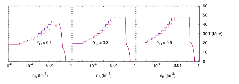
Figure 1: (color online) The lines delimit the regions in temperature and baryon number density for which the overall hyperon fraction exceeds $10^{-4}$, which are situated above the lines. The dark thick purple line corresponds to the BHB$\Lambda\phi$ model and light thin red line to the DD2Y model. Different charge fractions are shown as indicated within the panels.

In some parts of the $T$-$n_{B}$ diagram, however, a transition from inhomogeneous matter directly to hyperonic homogeneous matter is observed. This is the case at low densities and high temperatures, i.e. the density regions up to the bumps in Fig. 1. There, light clusters compete with hyperonic degrees of freedom with only very small differences in free energy which are of the order of the numerical accuracy of the EoS calculation. To technically construct the transition in this region, we follow a similar prescription as in Ref. Banik et al. (2014) and introduce a threshold value for the total hyperon fraction, $Y_{\mathit{hyperons}}=\sum_{j\in B_{Y}}n_{j}/n_{B}$. We let hyperonic matter appear only if $Y_{\mathit{hyperons}}>10^{-6}$. Note that the hyperon fraction is not the same as the strangeness fraction, $Y_{S}$, defined as the sum of all particle fractions multiplied by their respective strangeness quantum numbers, $Y_{S}=\sum_{j\in B}S_{j}n_{j}/n_{B}$.

Although the above described procedure allows to construct a smooth transition between the different parts of the EoS, it is of course not completely consistent. In principle, whenever hyperons compete with light nuclear clusters, the free energy of the system should be minimized allowing simultaneously for all different possibilities, e.g. a coexistence of light clusters with hyperons. In view of the tiny differences in free energy and the small fractions of particles other than nucleons, electrons, and photons in the transition region, a completely consistent treatment is left for future work.

III Equation of state properties

III.1 Compatibility with constraints

The interaction between nucleons can be constrained by data of finite nuclei and nuclear matter properties. The latter are chosen in general as the coefficients of a Taylor expansion of the energy per baryon of isospin symmetric nuclear matter around saturation. Values with a reasonable precision can be obtained for the saturation density ($n_{\mathit{sat}}$), binding energy ($E_{B}$), incompressibility ($K$), symmetry energy ($E_{\rm sym}$) and its slope ($L$). In addition, much effort has been recently devoted to theoretical ab-initio calculations of pure neutron matter in order to constrain the equation of state. This is particularly interesting for the EoS of compact stars, completing the information about symmetric matter. The only robust constraint on the interactions at super-saturation density arises from the recent observation of two massive neutron stars, indicating the maximum mass of a cold, non- or slowly-rotating (therefore spherically symmetric) neutron star should be above $2M_{\odot}$. A summary and discussion of some of the most important available constraints can be found e.g. in Oertel et al. (2017).

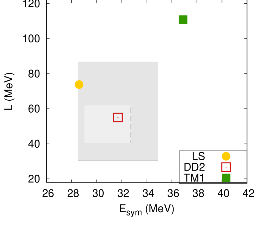
Figure 2: (color online) Values of $E_{\rm sym}$ and $L$ in different nuclear interaction models. The two gray rectangles correspond to the range for $E_{\rm sym}$ and $L$ derived in Ref. Lattimer and Lim (2013) (light Gray) and Ref. Oertel et al. (2017) (dark gray) from nuclear experiments and some neutron star observations.

The present parameterization, DD2, has been chosen since it agrees well with most of the established constraints. The values for $n_{\mathit{sat}}=0.149$ fm^-3, $E_{B}=16.0$ MeV and $K=243$ MeV are within standard ranges Oertel et al. (2017). The compatibility of $E_{\rm sym}$ and $L$ with ranges derived in Ref. Lattimer and Lim (2013) (light gray rectangle) and in Ref. Oertel et al. (2017) (dark gray rectangle), respectively, are shown in Fig. 2. For comparison we show the values for two other interactions, that of the Lattimer and Swesty EoS (LS) Lattimer and Swesty (1991) and that for the TM1 parameterization Sugahara and Toki (1994), too. These two interactions have been employed in other recently developed general purpose EoS, including non-nucleonic degrees of freedom, e.g. Ishizuka et al. (2008); Shen et al. (2011); Oertel et al. (2012).

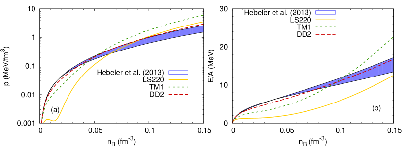
Figure 3: (color online) Pressure (left panel) and energy per baryon (right panel) of pure neutron matter as functions of baryon number density within different nuclear interaction models compared with the ab-initio calculations of Ref. Hebeler et al. (2013), indicated by the blue band.

In Fig. 3 pressure and energy per baryon for pure neutron matter are shown below saturation density. The blue band represents the results from the ab initio calculations from Ref. Hebeler et al. (2013) including an estimate of the corresponding uncertainties. In contrast to LS and TM1, the interaction DD2 employed here is in reasonable agreement with the ab initio calculations.

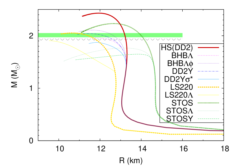
Figure 4: (color online) Gravitational mass versus circumferential equatorial radius for cold spherically symmetric neutron stars within different EoS models. The two horizontal bars indicate the two recent precise NS mass determinations, PSR J1614-2230 Demorest et al. (2010); Fonseca et al. (2016) (hatched gray) and PSR J0348+0432 Antoniadis et al. (2013) (green).

The mass-radius relation of cold spherically symmetric neutron stars within different general purpose EoS models is displayed in Fig. 4. Purely nucleonic versions are shown with solid lines, models including $\Lambda$-hyperons with dotted lines, and those including the entire baryon octet with dashed-dotted lines. These are the LS EoS Lattimer and Swesty (1991), its extension with $\Lambda$-hyperons (“LS220$\Lambda$”) Peres et al. (2013), the EoS by Shen et al. (“STOS”) employing the TM1 interaction Shen et al. (1998), its extension with $\Lambda$-hyperons (“STOS$\Lambda$”) Shen et al. (2011) and all hyperons (“STOSY”) Ishizuka et al. (2008), as well as the two models including $\Lambda$-hyperons within the same nuclear model as the present one from Ref. Banik et al. (2014), (“BHB$\Lambda$”) and (“BHB$\Lambda\phi$”). It is evident from the figure that there are only two EoSs including hyperons compatible with the $2M_{\odot}$-constraint: BHB$\Lambda\phi$ containing only $\Lambda$-hyperons and the present DD2Y. Both models are the same, except for the particle content. The additional hyperonic degrees of freedom in DD2Y slightly reduce the maximum mass with respect to BHB$\Lambda\phi$, but it remains above $2M_{\odot}$. The additional attractive $YY$-interaction in DD2Y$\sigma^{*}$ reduces the maximum mass to 1.87 $M_{\odot}$, thus slightly below the observational limit. A summary of cold neutron star properties for the different EoSs is given in Table 2.

III.2 Hyperon content and thermodynamic properties

As already mentioned in Ref. Oertel et al. (2016), the overall hyperon content within the EoS remains similar between the models containing only $\Lambda$-hyperons and the corresponding ones with the full baryonic octet. For cold NSs, this can be seen from Table 2. In Fig. 1, the regions where the overall hyperon fraction exceeds $10^{-4}$ are compared for BHB$\Lambda$ and DD2Y. Although, as expected, hyperons are slightly more abundant in the full model, the shape of the regions remains the same and only small quantitative differences are observed. The bump in the curves, i.e., the part of the lines above approximately 20 MeV, where the abundance of hyperons is still below $10^{-4}$, arises from the competition between light nuclear clusters and hyperons in this particular temperature and density domain and does not exist in the EoSs built on nuclear models without light clusters, see Ref. Oertel et al. (2017).

Model	$M_{g}^{\mathit{max}}$	$M_{B}^{\mathit{max}}$	$R_{1.4}$	$f_{S}$	$n_{B}^{(c)}$
	$[M_{\odot}]$	[$M_{\odot}$]	[km]		[fm-3]
HS(DD2)	2.43	2.90	13.27	-	0.84
BHB$\Lambda$	1.96	2.26	13.27	0.05	0.95
BHB$\Lambda\phi$	2.11	2.47	13.27	0.05	0.96
DD2Y	2.04	2.36	13.27	0.04	1.00
DD2Y$\sigma^{*}$	1.87	2.15	13.27	0.04	0.98

Table 2: Properties of cold spherically symmetric neutron stars in neutrinoless $\beta$-equilibrium: Maximum gravitational and baryonic masses, respectively, radius at a fiducial mass of $M_{g}=1.4M_{\odot}$, the total strangeness fraction, $f_{S}$, representing the integral of the strangeness fraction $Y_{S}/3$ over the whole star, defined as in Ref. Weissenborn et al. (2012), and the central baryon number density. The latter two quantities are given for the maximum mass configuration. In addition to the EoSs presented here, for comparison the values for the purely nucleonic version HS(DD2) Fischer et al. (2014) and the two versions including only $\Lambda$-hyperons from Ref. Banik et al. (2014) are listed.

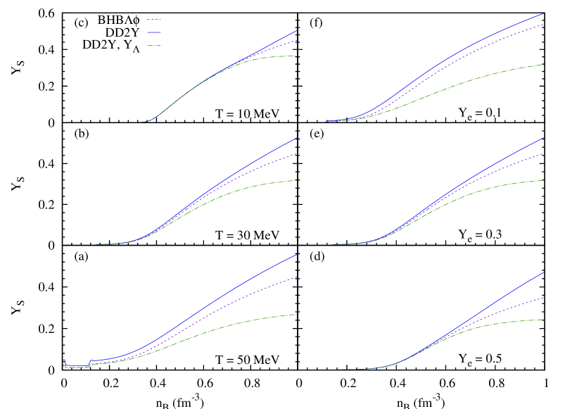
Figure 5: (color online) Total strangeness fraction as function of baryon number density for different values of fixed temperature and electron fraction $Y_{e}$ within BHB$\Lambda\phi$ (dotted lines) and DD2Y (solid lines) EoS. In panels (a-c), $Y_{e}=0.3$ and in panels (d-f), $T=30$ MeV. For information, the $\Lambda$-fraction in model DD2Y is indicated, too (dash-dotted lines).

In Fig. 5, the overall strangeness fraction is shown as function of baryon number density for different values of fixed temperature and electron fraction for both models, BHB$\Lambda\phi$ and DD2Y. As mentioned before, the hyperon onset density remains similar in both models and the decrease in $\Lambda$-fraction in DD2Y with respect to BHB$\Lambda\phi$ at high densities is compensated by the presence of other hyperons such that the overall strangeness fraction is larger in DD2Y. Note that here the strangeness fraction $Y_{S}$ has been taken and not the hyperon fraction. Naturally, the difference between both models increases with increasing temperature. With increasing $Y_{e}$, as expected, in both models the overall strangeness fraction decreases. The effect is, however, less pronounced in DD2Y since the population of neutral cascades and $\Sigma^{+}$ compensates partially the suppression of other hyperonic degrees of freedom.

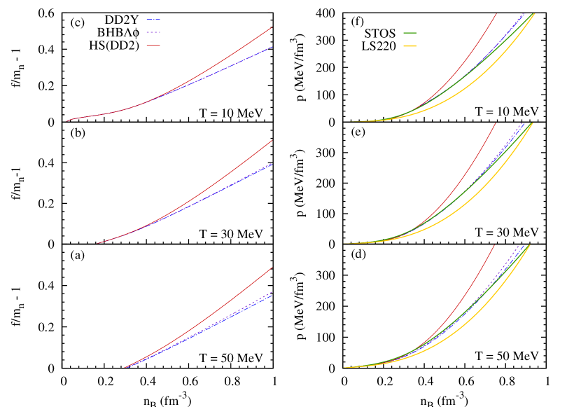
Figure 6: (color online) Pressure (panels d-f) and normalised free energy per baryon (panels a-c) as function of baryon number density for different values of fixed temperature and $Y_{e}=0.3$ within the three different EoS, HS(DD2), BHB$\Lambda\phi$ and DD2Y. For information, the pressure in the classical models LS220 and STOS is displayed, too.

Pressure and free energy per baryon are considerably reduced above roughly 2-3 times nuclear saturation density in the models with hyperons compared with the purely nucleonic HS(DD2) EoS, see Figs. 6 and 7. It is not surprising that the reduction is most important for high temperatures and low electron fractions. The presence of the full baryon octet in DD2Y leads only to a small further reduction with repsect to the model BHB$\Lambda\phi$, containing only $\Lambda$-hyperons. This is due to the fact that the overall hyperon fraction is very similar in both models, see the discussion above.

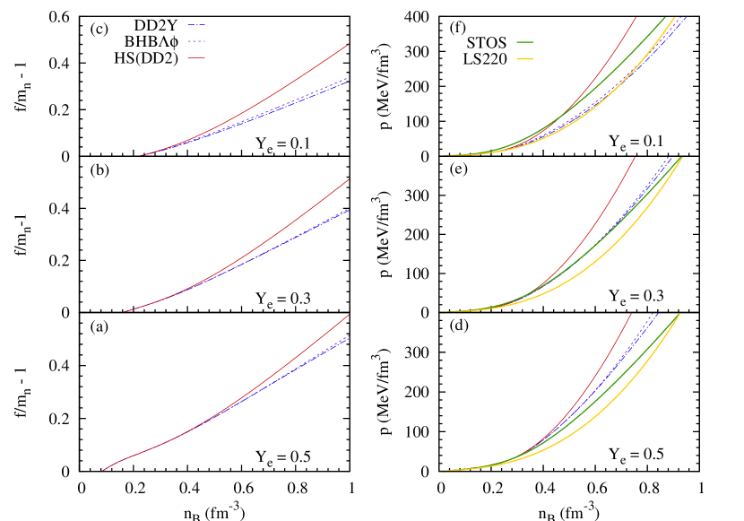
Figure 7: (color online) Same as Fig. 6, but for $T=30$ MeV and different fixed values of $Y_{e}$.

IV Temperature dependent stellar structure

In this section, we describe our strategy to solve for the star’s structure, following Ref. Villain et al. (2004). Equilibrium equations will be solved together with Einstein equations, assuming stationarity and axisymmetry. In addition, the matter content (represented by the energy momentum tensor) should fulfill the circularity condition, i.e. the absence of meridional convective currents. An EoS will close the system of equations. In full generality the EoS depends on temperature and on the different particle number densities or thermodynamically equivalent variables. Conditions for electromagnetic and strong equilibrium reduce the number of degrees of freedom in the EoS to three, related to baryon number density $n_{B}$, electron number density $n_{e}$ and temperature $T$. In neutron stars older than several minutes, the temperature can be considered as vanishing and neutrinoless weak $\beta$-equilibrium is achieved, such that the EoS becomes effectively barotropic, i.e. depends only on baryon number density or a thermodynamically equivalent variable. Neither in PNSs nor in merger remnants these conditions are fulfilled and in particular a nonzero temperature has to be considered.

Here, we will allow for an EoS with an explicit temperature dependence. Under the current assumptions, in particular stationarity, the most general solution for the star’s structure becomes again barotropic, and a relation $T(n_{B})$ (or thermodynamically equivalent) has to be provided Goussard et al. (1998, 1997); Villain et al. (2004). For simplicity we will restrict the results within the present work either to neutrinoless $\beta$-equilibrium or to a constant lepton fraction $Y_{L}=(n_{e}+n_{\nu})/n_{B}=n_{L}/n_{B}$ ($n_{\nu}$ and $n_{L}$ being, respectively, neutrino and lepton number densities). Following the standard presentation of the formalism (see e.g. Bonazzola et al. (1993); Villain et al. (2004)), Latin letters $i,j,\dots$ are used for spatial indices only, whereas Greek letters $\alpha,\beta,\dots$ denote spacetime indices.

IV.1 Einstein equations

General-relativistic models shall be described within the 3+1 formulation, where spacetime is foliated by a family of spacelike hypersurfaces $\Sigma_{t}$, labeled by the time coordinate $t$. Introducing coordinates ($x^{i}$) on each hypersurface, the line element can be written as

$$ds^{2}=-N^{2}dt^{2}+\gamma_{ij}\left(dx^{i}+\beta^{i}dt\right)\left(dx^{j}+\beta^{j}dt\right)~{}.$$ (18)

$N$ represents the lapse function, $\beta^{i}$ the shift vector and $\gamma_{ij}$ the 3-metric on each hypersurface $\Sigma_{t}$, thus defining the spacetime metric $g_{\alpha\beta}$. More details can be found e.g. in Gourgoulhon (2012).

The assumptions of stationarity, axisymmetry and asymptotic flatness imply the existence of two commuting Killing vector fields, given as $\vec{\zeta}=\partial/\partial_{t}$ and $\vec{\chi}=\partial/\partial_{\varphi}$ in an adapted coordinate system $(t,x^{1},x^{2},\varphi)$. The two remaining coordinates are chosen to be spherical, i.e. $x^{1}=r,x^{2}=\theta$. These adapted coordinates simplify the expression of the metric: $\beta^{r}=\beta^{\theta}=0$ and $\gamma_{r\varphi}=\gamma_{\theta\varphi}=0$. Finally, following Bonazzola et al. (1993); Villain et al. (2004) we use a quasi-isotropic gauge, which additionally gives $\gamma_{r\theta}=0$, such that the line element (18) becomes

$$ds^{2} = -N^{2}dt^{2}+A^{2}\left(dr^{2}+r^{2}d\theta^{2}\right)$$ (19)

$$+B^{2}r^{2}\sin^{2}\theta\left(d\varphi^{2}+\beta^{\varphi}dt\right)^{2},$$

with the notations $A^{2}=\gamma_{rr}=\gamma{\theta\theta}/r^{2}$ and $B^{2}=\gamma_{\varphi\varphi}/(r^{2}\sin^{2}\theta)$. All the metric potentials $\left(N,\beta^{\varphi},A,B\right)$ are functions of the coordinates $(r,\theta)$ only. Einstein equations for these four gravitational potentials, under our symmetry assumptions, reduce to a set of four elliptic (Poisson-like) partial differential equations, in which source terms contain both contributions from the energy-momentum tensor (matter) and non-linear terms with non-compact support, involving the gravitational field itself. Explicit expressions and discussion of these equations can be found in Bonazzola et al. (1993).

IV.2 Equilibrium equations

Matter is described as a perfect fluid with an energy-momentum tensor of the form

$$T^{\alpha\beta}=(\varepsilon+p)\,u^{\alpha}u^{\beta}+p\,g^{\alpha\beta}~{}.$$ (20)

$\varepsilon$ denotes here the total energy density (including rest mass), $p$ the pressure, and $u^{\alpha}$ is the fluid four-velocity; the fluid angular velocity is then defined as $\Omega:=u^{\varphi}/u^{t}$. We also introduce the pseudo-log enthalpy

$$H=\ln\left({\frac{\varepsilon+p}{m_{B}\,n_{B}}}\right)~{},$$ (21)

with $m_{B}$ a constant mass, where we chose the value $m_{B}=939.565$ MeV. Conservation of the energy-momentum tensor $\nabla_{\alpha}T^{\alpha\beta}=0$ yields the equation for the fluid equilibrium Goussard et al. (1998, 1997)

$$\partial_{i}\left(H+\ln N-\ln\Gamma\right)=\frac{Te^{-H}}{m_{B}}\partial_{i}s_{B}-u_{\varphi}u^{t}\partial_{i}\Omega~{}.$$ (22)

$\Gamma=Nu^{t}$ represents the Lorentz factor of the fluid with respect to the Eulerian observer and $s_{B}$ the entropy per baryon in units of the Boltzmann constant.

In this work, we will restrict ourselves only to the case where matter is rigidly rotating ($\Omega=\textrm{const}$), which means that the last term in Eq. (22) is zero. This equation is then integrable in three cases. First, for a constant $s_{B}$, which is in particular the case at zero temperature. The second case is the isothermal one (constant $T^{*}=TN/\Gamma$) defined in Ref. Goussard et al. (1998). Finally, the most general solution in rigid rotation is found introducing the heat function Villain et al. (2004)

$$\hat{H}(n_{B})=\int_{0}^{n_{B}}\frac{dp}{dn}\frac{1}{\varepsilon(n)+p(n)}dn~{},$$ (23)

where a parameterization $T(n_{B})$ has been assumed such that the EoS effectively is again barotropic. Using $\hat{H}$, the equilibrium condition reduces to:

$$\hat{H}+\ln N-\ln\Gamma=\textrm{const.},$$ (24)

which is pretty similar to the zero-temperature case Bonazzola et al. (1993). It is obvious that the heat function $\hat{H}$ reduces to the pseudo-log enthalpy $H$ at zero temperature, up to a constant factor of $\ln(m_{B}/\mu_{B}(n_{B}=0))$, which can be absorbed in the r.h.s of Eq. (24). For differentially rotating stars, allowing the rotation law to depend on the entropy profile, in principle, the condition of the EoS being barotropic could be relaxed. Such a scheme is, however, beyond the purpose of the present paper.

We have implemented the above described scheme, with a temperature dependent EoS within the numerical library lorene Gourgoulhon et al. (2016), see also refs. Bonazzola et al. (1993); Villain et al. (2004). The resolution of elliptic-type partial differential equations (Einstein equations in our case) is based on multi-domain spectral methods Grandclément and Novak (2009) and is widely used for the computation of stationary rotating compact objects. The equilibrium condition (24) is integrated in a straightforward way and the heat function (23) computed using the trapezoidal rule. Finally, we can use either an analytic (polytropic type) EoS or a tabulated realistic one, which is interpolated in a thermodynamically consistent way using the scheme by Swesty Swesty (1996).

Input parameters for a rigidly rotating neutron star model are: a temperature vs. density profile, a prescription for the lepton fraction (either $\beta$-equilibrium or constant $Y_{L}$), an EoS, a central value for the heat function $\hat{H}(r=0)$ and a value for the rotation frequency $\Omega$. We can then compute the numerical solution of all field equations described above and deduce global quantities such as gravitational mass $M_{g}$ (from the asymptotic behavior of the gravitational potential $N$), angular momentum $J$ (from the asymptotic behavior of the gravitational potential $\beta^{\varphi}$), or circumferential equatorial radius (from the integration of the line element (19) along the star’s equator). More details about these calculations can be found in Bonazzola et al. (1993).

V Models of hot stars

Within this section we will discuss results for both non-rotating (maximal masses, Sec. V.1) and rotating ($I$-$Q$ relations, Sec. V.2) stars with nonzero temperatures, employing different microscopic EoSs exposed in the preceding sections. For the study of their properties, $Y_{Q}$ will be fixed either by the condition of $\beta$-equilibrium and assuming that neutrinos freely leave the system, i.e. a vanishing electron lepton number chemical potential

$$\mu_{L}=0~{},$$ (25)

or by fixing the electron lepton fraction $Y_{L}=0.4$. This value lies slightly above typical values obtained from simulations, see e.g. Pons et al. (2001). We have chosen it in order to maximize the differences to the $\beta$-equilibrated case and thus show the maximal effect we would expect from composition. Muons will not be considered, although they might have a non-negligible influence on the EoS at the very center of the PNS Oertel et al. (2012). Neither of these conditions might be very realistic, since the hydrodynamic evolution should be coupled to neutrino transport, fixing the corresponding evolution of $Y_{e}=Y_{Q}$ inside the star. A more complete study of PNS evolution, combining our models with neutrino transport, is left for future work.

Hence, we do certainly not pretend to give a completely realistic picture of a PNS or a merger remnant. This simplified setup is nevertheless sufficient for the purpose of the present study, namely to demonstrate the usability of the newly developed EoS within a numerical code, and to get some ideas about the influence of hyperons on the properties of hot stars. Results with different temperature profiles will be presented: either yielding constant values of entropy per baryon, $s_{B}$, or profiles shown in Fig. 8 (left panel), inspired by realistic calculations of PNS evolution. Profile $T_{1}$ is within the range of values from the “canonical” simulations of cooling PNSs Pons et al. (1999). The maximum temperatures of profile $T_{2}$ is slightly above typical values from the aforementioned simulations and corresponds to values reached for a PNS formed in the collapse of a very massive progenitor star, close to the eventual collapse to a black hole, see, e.g., Fig. 16 of Ref. Hempel et al. (2012). Analytic expressions for both temperature profiles are given in appendix B. The corresponding entropy profiles are displayed in the right panel of Fig. 8.

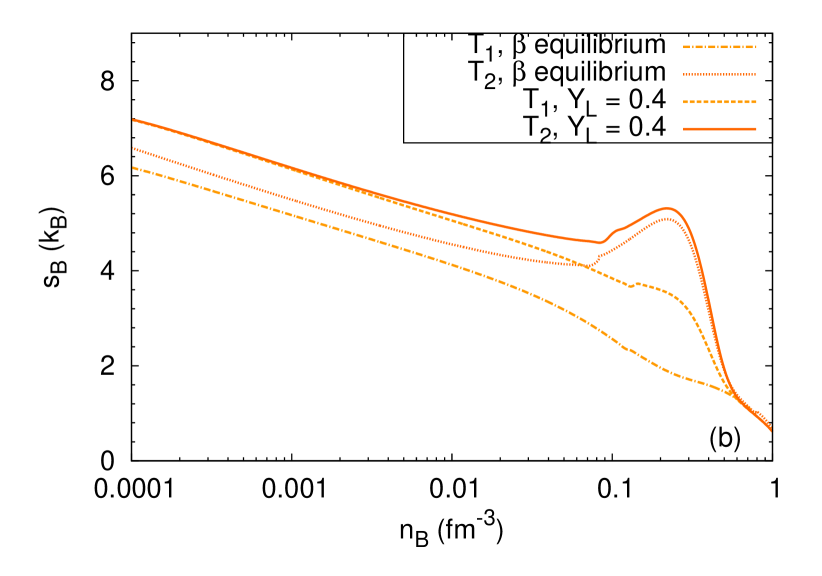
Figure 8: Left: $T(n_{B})$ relations used for the computation of hot star models. For comparison, the profiles obtained for different values of constant $s_{B}$ within the DD2Y EoS are shown, too. Right: $s_{B}(n_{B})$ resulting from the two chosen $T(n_{B})$ relations within the DD2Y EoS.

V.1 Maximal masses of non-rotating hot stars

The maximum baryonic mass a hot star can support is interesting both for the merger remnant of a binary coalescence, and for the PNS after the bounce occurs in a core collapse event, in order to determine the conditions for the formation of a black hole. Different mechanisms were evoked for stabilizing these objects against collapse to a black hole. First, these objects are supposed to be rotating and, as rotational effects on the maximum mass have been examined elsewhere, see e.g. Ref. Goussard et al. (1998, 1997); Kastaun and Galeazzi (2015), we do not discuss them here. In addition, for the merger remnant and the PNS in the case of collapse of fast spinning progenitor stars, the rotation profile is strongly differential. Although it is not clear what are the time scales driving toward rigid rotation, strong differential rotation can help in supporting very massive configurations Baumgarte et al. (2000); Morrison et al. (2004); Kastaun and Galeazzi (2015).

Next, in PNSs, the lepton rich environment certainly contributes to support a higher mass Prakash et al. (1997); Pons et al. (1999) and it is not only the cooling, but also the deleptonization via neutrino emission of the star which causes a potential collapse to a black hole. In a merger remnant, which is supposed to be close to $\beta$-equilibrium, this mechanism cannot play the same role. Finally, canonical calculations suggested that thermal pressure is unlikely to be able to to stabilize the star Prakash et al. (1997); Pons et al. (1999); Kaplan et al. (2014), it might even slightly reduce the maximum mass due to the population of additional degrees of freedom at finite temperature. However, these studies were restricted to rather low entropy values. For PNSs formed in core-collapse of massive progenitors, which eventually are expected to collapse to a black hole, it was found in Refs. Hempel et al. (2012); Steiner et al. (2013) that thermal effects can increase the maximal gravitational mass by up to 0.6 $M_{\odot}$, where neutrinoless $\beta$-equilibrium and a constant entropy per baryon of $s_{B}=4$ was considered.

When studying the maximum mass, previous works were considering cold stars Salgado et al. (1994); Morrison et al. (2004), or a very restricted set of EoS, containing only homogeneous matter Prakash et al. (1997); Pons et al. (1999) or only nucleonic matter Hempel et al. (2012); Steiner et al. (2013); Kaplan et al. (2014); Kastaun and Galeazzi (2015). Our new EoS including hyperonic degrees of freedom allows to check the influence of these new degrees of freedom on the mass, treating consistently nuclear clustering at low densities and temperatures. A recent study of PNSs with EoSs containing anti-kaons can be found in Ref. Batra et al. (2017).

	$S=0M_{\odot}$		$S=3M_{\odot}$			$S=5M_{\odot}$			$S=7M_{\odot}$			$S=9M_{\odot}$
	$M_{g}^{\mathit{max}}$	$M_{B}^{\mathit{max}}$	$M_{g}^{\mathit{max}}$	$M_{B}^{\mathit{max}}$	$T^{(c)}$	$M_{g}^{\mathit{max}}$	$M_{B}^{\mathit{max}}$	$T^{(c)}$	$M_{g}^{\mathit{max}}$	$M_{B}^{\mathit{max}}$	$T^{(c)}$	$M_{g}^{\mathit{max}}$	$M_{B}^{\mathit{max}}$	$T^{(c)}$
Model
	($M_{\odot}$)	($M_{\odot}$)	($M_{\odot}$)	($M_{\odot}$)	(MeV)	($M_{\odot}$)	($M_{\odot}$)	(MeV)	($M_{\odot}$)	($M_{\odot}$)	(MeV)	($M_{\odot}$)	($M_{\odot}$)	(MeV)
HS(DD2)	2.42	2.90	2.43	2.88	41	2.43	2.83	68	2.45	2.77	90	2.50	2.73	108
BHB$\Lambda\phi$	2.11	2.47	2.11	2.42	41	2.13	2.39	67	2.18	2.37	91	2.27	2.39	107
DD2Y	2.04	2.35							2.02	2.15	81	2.11	2.17	96
HS(DD2)	-	-	2.37	2.70	32	2.38	2.67	53	2.40	2.64	71	2.44	2.61	89
BHB$\Lambda\phi$	-	-	2.17	2.42	27	2.18	2.39	49	2.21	2.37	65	2.27	2.36	86
DD2Y	-	-	2.17	2.43	22	2.16	2.36	39	2.16	2.30	55	2.20	2.27	70

Table 3: Maximum gravitational and baryonic masses in units of solar mass for non-rotating stars and different values of constant total entropy. The central temperature of the maximum mass configuration is given, too. Since the entropy per baryon, $s_{B}$, is constant for each configuration, its value for the respective maximum mass configurations can be obtained simply by dividing $S$ by $M_{B}^{\mathit{max}}$, see Eq. (27). The upper part assumes neutrinoless $\beta$-equilibrium and in the lower part $Y_{L}=0.4$. For sake of an easier comparison the maximum masses in the cold $\beta$-equilibrated case are recalled in the first two columns. No values are given for DD2Y and the $\beta$-equilibrated case at $S=3M_{\odot}$ and $S=5M_{\odot}$ since at high central densities the electron fraction lies below the limiting value of the table ($Y_{e}<0.01$). The corresponding curves in Fig. 9 do not show a maximum, we could thus not determine the maximum masses.

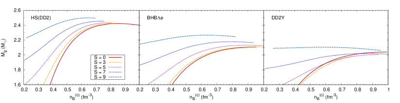
Figure 9: Gravitational mass versus central baryon number density for non-rotating stars for three different EoSs, without hyperons (left), with $\Lambda$-hyperons (middle) and the complete baryon octet (right). Different values of constant total entropy $S$ have been used, indicated in units of solar masses. $\beta$-equilibrium has been assumed. For comparison, the cold result is shown, too. For DD2Y, at $S=3M_{\odot}$ and $S=5M_{\odot}$, the curves end at some central density above which no longer any $\beta$-equilibrated solution is found. The reason is that the electron fraction becomes lower than the limiting value of the EoS table ($Y_{e}=0.01$). No maximum could be determined in this case.

In order to discuss maximum masses, we have to consider the stability of the computed stellar configurations. At zero temperature for non-rotating stars, stable configurations verify simply $dM_{g}/dn_{B}^{(c)}\geq 0$. This criterion is a special case of the result by Friedman et al. Friedman et al. (1988), who have established a turning point criterion for determining whether a rotating star becomes secularly unstable with respect to axisymmetric perturbations. Here, we have to use an extended version for hot (non-rotating) stars.

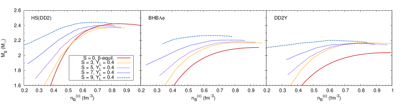
Figure 10: Same as Fig. 9, comparing stars with $Y_{L}$ = 0.4 at different constant total entropy values with the $\beta$-equilibrated result for cold stars.

For the following considerations, we will consider a more general case for hot rotating stars and we will denote by $J$ the total angular momentum of the star and $S$ the total entropy. $J$ is defined as Bonazzola et al. (1993)

$$J=\int A^{2}B^{2}(E+p)Ur^{3}\sin^{2}\theta drd\theta d\phi~{}.$$ (26)

$E$ denotes the energy density as measured by a locally non-rotating observer, $E=\Gamma^{2}(\varepsilon+p)-p$, and $U$ the fluid velocity as measured by the same observer. The latter is related to the factor $\Gamma$ as $\Gamma=(1-U^{2})^{-1/2}$. $S$ can be expressed in a similar way from

$$S=\int A^{2}B\Gamma n_{B}s_{B}m_{B}r^{2}\sin\theta drd\theta d\phi~{}.$$ (27)

As shown in Ref. Goussard et al. (1998), based on the work by Sorkin Sorkin (1982), a meaningful criterion for a configuration being secularly stable can be obtained for rigidly rotating stars with a constant $s_{B}$ (or $T^{*}$) throughout the star. In the former case, i.e. for constant $s_{B}$, the total entropy is simply given by $S=s_{B}\,M_{B}$. Following Ref.  Goussard et al. (1998), a star becomes unstable at the extremal points

$$\left(\frac{\partial J}{\partial n_{B}^{(c)}}\right)_{M_{B},S}=0\;,\;\left(\frac{\partial M_{B}}{\partial n_{B}^{(c)}}\right)_{J,S}=0\;,\;\left(\frac{\partial S}{\partial n_{B}^{(c)}}\right)_{M_{B},J}=0~{}.$$ (28)

Obviously, upon varying the central baryon number density (or equivalently the central heat function) at constant angular momentum, the rotation frequency changes, see e.g. the textbook Friedman and Stergioulas (2013), i.e. sequences at constant rotation frequency do not allow to distinguish stable from unstable solutions. Equivalently, for sequences at constant total entropy, the entropy per baryon $s_{B}$ is not constant, and sequences at constant $s_{B}$ do not allow to identify stable and unstable configurations.

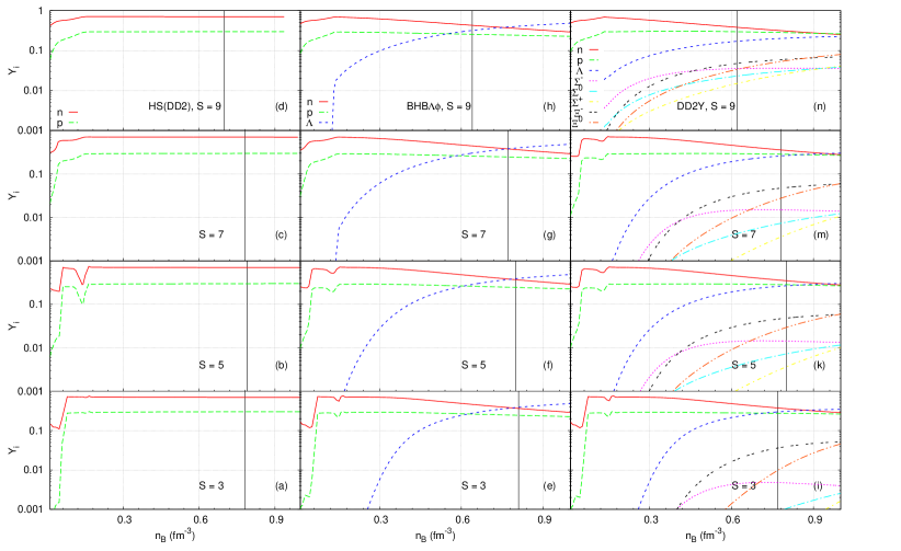
Figure 11: Particle fractions in hot neutron star matter for the three different EoS discussed here. The lepton fraction has been fixed to $Y_{L}=0.4$ and the entropy per baryon corresponds to the value of the respective maximum mass configuration with the total entropy indicated in each panel. The vertical lines show the central density of the respective maximum mass configurations.

We are mainly interested here in thermal effects on the star’s mass, corresponding to the maximum mass a cooling star can support, i.e. the second criterion of Eq. (28) is the most interesting one. It determines the maximum mass at different given values of constant total entropy and angular momentum. In the following, we restrict the discussion to non-rotating stars, for which $J=0$ and is therefore constant. Since the criterion for distinguishing secularly stable from unstable configurations is meaningful only for constant $s_{B}$ (or $T^{*}$), we will restrict our investigations of maximum masses to models with constant $s_{B}$, too.

The different values of the maximum mass are summarized in Table 3. In the upper part, neutrinoless $\beta$-equilibrium is assumed, in the lower part a constant $Y_{L}=0.4$.

V.1.1 Thermal effects

In Fig. 9 we thus display the gravitational mass versus central baryon number density obtained for non-rotating stars and different values of total entropy $S$. Results for three different EoSs are shown: the purely nucleonic one, HS(DD2), the one containing $\Lambda$-hyperons, BHB$\Lambda\phi$, and the new EoS considering the entire baryon octet, DD2Y. We do not show results for DD2Y$\sigma^{*}$ here since it does not respect the cold neutron star maximum mass constraint. $\beta$-equilibrium is assumed for all calculations.

It is obvious that for $S=3M_{\odot}$, corresponding to configurations with $s_{B}$ roughly between 1 and 2, thermal effects on the maximum mass are small, and almost no difference can be observed with respect to the result for cold stars. A slight reduction of the gravitational mass for BHB$\Lambda\phi$ and, in particular, DD2Y, is due to the population of additional degrees of freedom at finite temperature for these two EoSs allowing for non-nucleonic particles. These findings confirm previous investigations, see e.g. Refs. Prakash et al. (1997); Pons et al. (1999); Kaplan et al. (2014). At low central densities, thermal effects are more important. This can be understood since for total entropy constant, with decreasing gravitational mass, the entropy per baryon $s_{B}$ of the configurations increases, reaching almost $s_{B}=3$ at the lower end of the curves, modifying considerably the EoS.

In contrast, at $S=9$, thermal effects on the gravitational masses are clearly non-negligible for all three EoS. The maximum mass is increased by 4% for HS(DD2), 8% for BHB$\Lambda\phi$ and 7% for DD2Y, respectively. These values are of the same order as those expected for rigid rotation Bonazzola et al. (1993). The temperatures and entropies of these configurations are reached typically for PNSs in the post-bounce phase of core-collapse events with massive progenitors. The importance of thermal effects can be seen also from the shift in central density of the maximum mass configurations compared with the cold result. The central density is reduced with increasing value of $S$ since the hot star becomes less compact due to thermal excitations.

It should be pointed out that for a given entropy per baryon the temperature is significantly lower within an EoS including hyperons than in a purely nuclear one, see e.g. Oertel et al. (2016). This is a trivial thermodynamic effect: the appearance of hyperons implies that the energy is shared among an increased number of degrees of freedom, with consequently reduced thermal excitations for each of them. Therefore, although the value of $s_{B}$ for the maximum mass configurations is higher for the EoS with hyperons than for the purely nuclear one, the central temperature with DD2Y is only 96 MeV, whereas it is 108 MeV for HS(DD2).

V.1.2 Composition

It is known that a lepton rich environment disfavors hyperonic degrees of freedom and that generally with increasing hadronic charge fraction, $Y_{Q}$, the EoS becomes stiffer due to the reduced number of degrees of freedom present Prakash et al. (1997); Pons et al. (1999); Colucci and Sedrakian (2013); Oertel et al. (2017, 2016). Therefore neutrino trapping has been evoked for a long time already as one of the main mechanisms to stabilize a PNS with hyperons (or pions/kaons) against collapse to a black hole. From Fig. 10 it is evident that our results confirm previous findings. We display the gravitational mass of non-rotating stars as function of central baryon number density for the three previously considered EoSs. A fixed lepton fraction of $Y_{L}=0.4$ and high temperatures ($S=9$) or low temperatures ($S=3$) is compared with the respective $\beta$-equilibrated results for cold stars.

As expected, for DD2Y, the lepton rich environment with $Y_{L}=0.4$ clearly contributes to increasing considerably the gravitational mass supported by the star. To less extent, this is true for BHB$\Lambda\phi$, too. The difference between DD2Y and BHB$\Lambda\phi$ becomes small since $\Lambda$-hyperons, being charge neutral, are less affected by the higher electrons fraction than charged hyperons, essentially $\Sigma^{-}$. In contrast, for the purely nucleonic EoS HS(DD2) almost no difference between the lepton rich and the $\beta$-equilibrated case is observed at $S=3$ and only a moderate increase for $S=9$. The combination of thermal and composition effects leads to a maximum mass of $M_{g}=2.2M_{\odot}$ for DD2Y with $S=9$ and $Y_{L}=0.4$, $0.16M_{\odot}(\approx 8\%)$ above the cold $\beta$-equilibrated maximum mass.

It should be noted, however, that with increasing temperature the hyperon suppression in a lepton rich environment becomes less pronounced. Therefore, for DD2Y –and to less extent for BHB$\Lambda\phi$, too– the increase in maximum gravitational mass with increasing total entropy is moderate at $Y_{L}=0.4$. This can be seen from Fig. 11, too, where the different particle fractions for the maximum mass configurations are shown. For $S=9$, corresponding to $s_{B}=3.96$ with DD2Y, all different hyperonic species have non-negligible fractions at the center of the star due to the high temperatures reached.

V.2 $I$-$Q$-relation

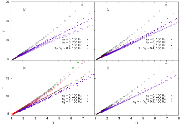
Figure 12: (color online) Normalized moment of inertia versus quadrupole moment for different EoS. The color coding corresponds to different EoS models whereas different symbols indicate rotation frequencies and entropy per baryon of the stars. In panel (a) different nucleonic and hyperonic EoS are shown for cold stars, in $\beta$-equilibrium, for the slow as well as fast rotating case, respectively. The LS220 EoS and the counterpart with $\Lambda$-hyperons are thereby shown by red symbols, STOS EoS with and without hyperons by green symbols and the three EoSs based on DD2, HS(DD2), BHB$\Lambda\phi$ and DD2Y, by violet symbols. For the latter three EoS in addition the results for slow rotating configurations with $s_{B}=4$ are displayed. In the three other panels the cold reference case with the HS(DD2) EoS is displayed by black symbols and different situations are considered with the three EoSs, HS(DD2), BHB$\Lambda\phi$, and DD2Y, indicated by violet symbols: constant $Y_{L}=0.4$ (b), profile $T_{2}$ (c), profile $T_{1}$ (d).

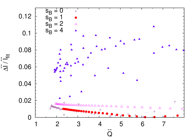
Figure 13: (color online) Relative difference between Eq. (29) – the fitted results for cold slowly rotating stars– and the results at different constant $s_{B}$ values for the DD2Y EoS, assuming neutrinoless $\beta$-equilibrium.

It has been shown Yagi and Yunes (2013a, b) that there exist relations between the moment of inertia ($I$), the tidal deformability ($\lambda$) and the quadrupole moment ($Q$) of neutron stars which are approximately independent of the internal composition and the EoS. Originally proposed for slowly rotating cold neutron stars, they remain EoS independent for fast rotation, too, and universal fits with a functional form

$$\ln y=a+b\,\ln x+c\,(\ln x)^{2}+d\,(\ln x)^{3}+e\,(\ln x)^{4}$$ (29)

can be established Yagi and Yunes (2013a, b). The coefficients $a,b,c,d,e$ are frequency dependent Doneva et al. (2013) but do not depend on the EoS. $x$ and $y$ represent any couple of the normalized quantities $\bar{I},\bar{Q},\bar{\lambda}$

$$\bar{I}=\frac{I}{M^{3}_{g}}\quad,\quad\bar{Q}=\frac{Q}{M^{3}_{g}(J/M^{2}_{g})^{2}}\quad,\quad\bar{\lambda}=\frac{\lambda}{M^{5}_{g}}~{},$$ (30)

with $M_{g}$ being the star’s gravitational mass and $J$ its angular momentum. We will employ here the numerical values for the fit coefficients obtained from a fit to the results for cold stars with the APR EoS Akmal et al. (1998), reference EoS in most papers in the literature. They are listed in table 4.

$a$	$b$	$c$	$d$	$e$
1.5196	0.4372	0.0687	0.013	0.000897

Table 4: Values of the fit parameters in Eq. (29) relating the normalized moment of inertia and quadrupole moment obtained from the results for cold slowly rotating neutron stars with the APR EoS Akmal et al. (1998).

Considering the difficulty of defining Love numbers for the case of a rapidly spinning object (see e.g. Pani et al. Pani et al. (2015)), we will focus here on the $\bar{I}$-$\bar{Q}$ relation. Nevertheless, a loss of universality in this relation would imply a loss of universality in the more general $\bar{I}$-$\bar{\lambda}$-$\bar{Q}$, too. The results for different EoSs are shown in Fig. 12.

Results for cold stars are shown in panel (a), for slow and fast rotating stars, see the symbols for $s_{B}=0$. Different colors represent different EoSs. In addition to the classical nuclear LS and STOS EoSs, we include other general purpose models, not only purely nucleonic but, respectively, with $\Lambda$-hyperons and the entire baryon octet, too, always assuming neutrinoless $\beta$-equilibrium. The present results, considering in addition hyperonic EoSs, clearly confirm previous findings that $I$-$Q$ relations are independent of the EoS with frequency dependent fit coefficients Doneva et al. (2013).

In Ref. Martinon et al. (2014) a study of this relation has been performed, employing purely nuclear EoSs from Refs. Pons et al. (1999, 2001), this time assuming different realistic entropy per baryon and electron fraction profiles for the PNS evolution during the minute following bounce. The main result the authors found was that universality of the so-called $I$-Love-$Q$ relations is violated in the early phases of PNS evolution and recovered as soon as the entropy gradients smoothen out and the star becomes more or less isentropic. It should then be independent of the exact value of $s_{B}$.

Our results including hyperonic EoS confirm that indeed, the $\bar{I}$-$\bar{Q}$-relation for an isentropic star with $s_{B}=1$ or $s_{B}=2$ agrees with the result for cold stars. The same is true for fast rotation, and assuming $\beta$-equilibrium or a constant lepton fraction $Y_{L}$ does only induce a small scatter in the results. The results with constant $s_{B}=4$ – see panels (a) and (b) of Fig. 12 – although they remain universal in the sense that there is only a small difference between different EoS, deviate, however, clearly from the results for cold stars. This can be seen from Fig. 13, too, where we have plotted for the DD2Y EoS, the relative difference between the numerical results and the fit function of Eq. (29), $\Delta\bar{I}/\bar{I}_{\mathit{fit}}=(\bar{I}-\bar{I}_{\mathit{fit}})/\bar{I}_{\mathit{fit}}$ at different values of constant entropy per baryon. For $s_{B}=1$ or $s_{B}=2$, the deviations remain below 2%, whereas at $s_{B}=4$, they can exceed 10%.

Both temperature profiles with entropy gradients – see panels (c) and (d) – display obvious deviations from the results for cold stars, too. With increasing temperature, the differences induced by the lepton fraction increase, too.

In Ref. Martinon et al. (2014) the observed deviations from universality in the early stages of PNS evolution were attributed to the presence of entropy gradients. Our results suggest a slightly modified picture, in the sense that universality is not a question of entropy gradients, but of thermal effects. As we have seen also during the preceding discussion on maximum masses, at $s_{B}=1$ or $s_{B}=2$, which are typical values in the late stages of PNS evolution probed in Ref. Martinon et al. (2014), thermal effects on the EoS and thus on the star’s structure remain small. At higher entropies, thermal effects start to influence the EoS, thus the star’s structure and universality of $\bar{I}$-$\bar{Q}$ relations are modified. Such entropy values can be reached in PNSs or merger remnants, depending on many factors such as the progenitors, rotation or metallicity.

Since the $\bar{I}$-$\bar{Q}$ relation still seems independent of the employed EoS, it might be tempting to try to obtain another “universal” fit, depending this time on rotation frequency and entropy/temperature. In contrast to the former, neither temperature nor entropy of the star are quantities which are observationally accessible. Therefore such a law would not help for data analysis and we refrain from giving one here. Anyway, in view of the present results doubts are allowed concerning the relevance of $\bar{I}$-$\bar{Q}$ relations for analysis of PNS or merger remnant data, including gravitational wave signals from the last stages of binary neutron star mergers. Let us stress here that entropy values of the order of $s_{B}=4$ are quite realistic in such cases, see e.g. the simulations in Refs. Hempel et al. (2012); Steiner et al. (2013); Perego et al. (2014).

VI Summary and conclusions

In this paper we have presented a new consistent general purpose EoS, including in particular thermal effects. The new EoS, including the entire baryon octet, is compatible with present constraints from nuclear physics and neutron star observations. The complete new EoS as function of $T,n_{B},Y_{e}$ will be made publicly available in tabulated form on the Compose database Typel et al. (2015), see appendix A for details.

We have demonstrated the applicability of the new EoS, investigating maximum masses of hot stars, comparing a purely nuclear EoS with one including $\Lambda$-hyperons and the new one with all hyperons. To that end we have applied a numerical code able to provide stationary models of relativistic rotating stars, including the effect of nonzero temperature. The main motivation for studying hot (rotating) stars are the birth of neutron stars, i.e. the evolution of PNSs, and the neutron star created in the aftermath of a binary neutron star merger. In order to correctly identify the configurations which are secularly stable, we have constructed sequences at different values of constant total entropy, $S$, in contrast to many previous works considering constant entropy per baryon, $s_{B}$.

As we have seen, thermal effects, and a lepton rich environment can considerably increase the maximally supported mass to a degree depending on the EoS. The lepton rich environment is important in particular if hyperons are present. If the entropy per baryon exceeds roughly $s_{B}=2$, thermal effects become important in the EoS, too. Thus for a total entropy roughly above $5M_{\odot}$ thermal effects on the maximum mass become noticeable. These high temperatures can be reached in both merger remnants and PNSs depending on the particular conditions. Let us recall again that previous works Baumgarte et al. (2000); Morrison et al. (2004); Kastaun and Galeazzi (2015) suggest that the main effect stabilizing a merger remnant or a PNS above the maximum mass of its non-rotating cold neutrinoless $\beta$-equilibrated counterpart is differential rotation, which we did not consider here.

Following the work by Martinon et al. Martinon et al. (2014), the universality of $I$-$Q$ relations has been tested for fast rotating hot stars, retrieving their results that a low constant nonzero entropy does not modify the relations. Universality, tested before only for purely nuclear models, is maintained in the presence of hyperons, too. This is, however, no longer true if thermal effects in the EoS become non negligible, independently of the presence of entropy gradients, i.e., it also occurs for high, but constant entropies.

Appendix A Technical issues of the new EoS table

The new EoS in its version DD2Y is provided in a tabular form in the Compose data base, http://compose.obspm.fr as a function of $T,n_{B},Y_{e}$. The contribution from electrons is included. Note that the Compose software allows to calculate additional quantities such as, e.g., sound speed, from those provided in the tables. Please see the Compose manual Typel et al. (2015) and the data sheet on the web site for more details about the definition of the different quantities.

• The grid is specified as follows:

  	$T$	$n_{B}$	$Y_{e}$
  # of points	80	302	59
  Minimum value	0.1 MeV	$10^{-12}\mathrm{fm}^{-3}$	0.01
  Maximum value	158.5 MeV	$1.202~{}\mathrm{fm}^{-3}$	0.6
  Scaling	logarithmic	logarithmic	linear

• Thermodynamic quantities provided:

  1. Pressure divided by baryon number density $p/n_{B}$ [MeV]

  2. Entropy per baryon $s/n_{B}$

  3. Scaled baryon chemical potential $\mu_{B}/m_{n}-1$

  4. Scaled charge chemical potential $\mu_{Q}/m_{n}$

  5. Scaled (electron) lepton chemical potential $\mu_{L}/m_{n}$

  6. Scaled free energy per baryon $f/(n_{B}m_{n})-1$

  7. Scaled energy per baryon $e/(n_{B}m_{n})-1$

• Compositional data provided:

  1. Particle fractions of baryons and electrons, $Y_{i}=n_{i}/n_{B}$

  2. Particle fractions of deutons (²H), tritons (³H), ³He, and $\alpha$-particles (⁴He)

  3. Fraction of a representative (average) heavy nucleus, together with its average mass number and average charge

  Please note that only nonzero particle fractions are listed.

• Effective Dirac masses $M^{*}$ of all baryons with nonzero density are provided within homogeneous matter.

Appendix B Expressions for the temperature profiles

Although they are inspired by results from simulations, for computational simplicity, analytic parameterizations for the temperature profiles, $T_{1}$ and $T_{2}$, are employed of the form

$$T(n_{B})=c\,n_{B}^{\alpha}+d\,n_{B}+\frac{a\,n_{B}}{1+\exp(b\,(n_{B}-n_{0})^{2})}~{}.$$ (31)

$n_{0}$ indicates here the saturation density, $n_{0}=0.155\mathrm{fm}^{-3}$ and the values of the other parameters are listed below.

	$a$	$b$	$c$	$d$	$\alpha$
	(MeV fm3)	fm6	(MeV fm3α)	(MeV fm3)
$T_{1}$	10.01	26.21	77.39	-65.15	0.35
$T_{2}$	470.0	26.21	77.39	-65.15	$\frac{1}{3}$

References

- Burrows and Lattimer (1986) A. Burrows and J. M. Lattimer, Astrophys. J. 307, 178 (1986).
- Keil and Janka (1995) W. Keil and H. T. Janka, Astron. Astrophys. 296, 145 (1995).
- Pons et al. (1999) J. A. Pons, S. Reddy, M. Prakash, J. M. Lattimer, and J. A. Miralles, Astrophys. J. 513, 780 (1999).
- Baumgarte et al. (1996) T. W. Baumgarte, S. A. Teukolsky, S. L. Shapiro, H. T. Janka, and W. Keil, Astrophys. J. 468, 823 (1996).
- Pons et al. (2001) J. A. Pons, A. W. Steiner, M. Prakash, and J. M. Lattimer, Phys. Rev. Lett. 86, 5223 (2001).
- Ishizuka et al. (2008) C. Ishizuka, A. Ohnishi, K. Tsubakihara, K. Sumiyoshi, and S. Yamada, J. Phys. G 35, 085201 (2008).
- Sumiyoshi et al. (2009) K. Sumiyoshi, C. Ishizuka, A. Ohnishi, S. Yamada, and H. Suzuki, Astrophys. J. Lett. 690, L43 (2009).
- Nakazato et al. (2010) K. Nakazato, K. Sumiyoshi, and S. Yamada, Astrophys. J. 721, 1284 (2010).
- Nakazato et al. (2012) K. Nakazato, S. Furusawa, K. Sumiyoshi, A. Ohnishi, S. Yamada, and H. Suzuki, Astrophys. J. 745, 197 (2012).
- Hempel et al. (2012) M. Hempel, T. Fischer, J. Schaffner-Bielich, and M. Liebendörfer, Astrophys. J. 748, 70 (2012).
- Peres et al. (2013) B. Peres, M. Oertel, and J. Novak, Phys.Rev. D87, 043006 (2013).
- Steiner et al. (2013) A. W. Steiner, M. Hempel, and T. Fischer, Astrophys. J. 774, 17 (2013).
- Char et al. (2015) P. Char, S. Banik, and D. Bandyopadhyay, Astrophys. J. 809, 116 (2015).
- Ferrari et al. (2003) V. Ferrari, G. Miniutti, and J. Pons, Mon. Not. R. Astron. Soc. 342, 629 (2003).
- Sekiguchi et al. (2011) Y. Sekiguchi, K. Kiuchi, K. Kyutoku, and M. Shibata, Phys. Rev. Lett. 107, 051102 (2011).
- Prakash et al. (1997) M. Prakash, I. Bombaci, M. Prakash, P. J. Ellis, J. M. Lattimer, et al., Phys.Rept. 280, 1 (1997).
- Pons et al. (2001) J. A. Pons, J. A. Miralles, M. Prakash, and J. M. Lattimer, Astrophys.J. 553, 382 (2001).
- Pons et al. (2000) J. A. Pons, S. Reddy, P. J. Ellis, M. Prakash, and J. M. Lattimer, Phys.Rev. C62, 035803 (2000).
- Nicotra et al. (2006) O. E. Nicotra, M. Baldo, G. F. Burgio, and H.-J. Schulze, Phys. Rev. D 74, 123001 (2006).
- Menezes and Providencia (2007) D. P. Menezes and C. Providencia, (2007), arXiv:astro-ph/0703649 [astro-ph] .
- Dexheimer and Schramm (2008) V. Dexheimer and S. Schramm, Astrophys.J. 683, 943 (2008).
- Yasutake and Kashiwa (2009) N. Yasutake and K. Kashiwa, Phys. Rev. D 79, 043012 (2009).
- Bombaci et al. (2007) I. Bombaci, D. Logoteta, C. Providencia, and I. Vidana, Astron.Astrophys. 462, 1017 (2007).
- Burgio et al. (2011) G. F. Burgio, H.-J. Schulze, and A. Li, Phys. Rev. C83, 025804 (2011).
- Chen et al. (2012) H. Chen, M. Baldo, G. F. Burgio, and H.-J. Schulze, Phys. Rev. D 86, 045006 (2012).
- Botvina and Mishustin (2010) A. S. Botvina and I. N. Mishustin, Nucl. Phys. A 843, 98 (2010).
- Typel et al. (2010) S. Typel, G. Röpke, T. Klähn, D. Blaschke, and H. Wolter, Phys.Rev. C81, 015803 (2010).
- Hempel and Schaffner-Bielich (2010) M. Hempel and J. Schaffner-Bielich, Nucl. Phys. A837, 210 (2010).
- Shen et al. (2011a) G. Shen, C. J. Horowitz, and S. Teige, Phys. Rev. C 83, 035802 (2011a).
- Shen et al. (2011b) G. Shen, C. J. Horowitz, and E. O’Connor, Phys. Rev. C 83, 065808 (2011b).
- Raduta and Gulminelli (2010) A. Raduta and F. Gulminelli, Phys.Rev. C82, 065801 (2010).
- Furusawa et al. (2013) S. Furusawa, K. Sumiyoshi, S. Yamada, and H. Suzuki, Astrophys. J. 772, 95 (2013).
- Togashi et al. (2017) H. Togashi, K. Nakazato, Y. Takehara, S. Yamamuro, H. Suzuki, and M. Takano, Nucl. Phys. A961, 78 (2017).
- Furusawa et al. (2017) S. Furusawa, H. Togashi, H. Nagakura, K. Sumiyoshi, S. Yamada, H. Suzuki, and M. Takano, J. Phys. G44, 094001 (2017).
- Nakazato et al. (2008) K. Nakazato, K. Sumiyoshi, and S. Yamada, Phys. Rev. D 77, 103006 (2008).
- Sagert et al. (2009) I. Sagert, T. Fischer, M. Hempel, G. Pagliara, J. Schaffner-Bielich, A. Mezzacappa, F.-K. Thielemann, and M. Liebendörfer, Phys. Rev. Lett. 102, 081101 (2009).
- Shen et al. (2011) H. Shen, H. Toki, K. Oyamatsu, and K. Sumiyoshi, Astrophys.J.Suppl. 197, 20 (2011).
- Oertel et al. (2012) M. Oertel, A. Fantina, and J. Novak, Phys.Rev. C85, 055806 (2012).
- Gulminelli et al. (2013) F. Gulminelli, A. Raduta, M. Oertel, and J. Margueron, Phys.Rev. C87, 055809 (2013).
- Banik et al. (2014) S. Banik, M. Hempel, and D. Bandyopadhyay, Astrophys.J.Suppl. 214, 22 (2014).
- Demorest et al. (2010) P. Demorest, T. Pennucci, S. Ransom, M. Roberts, and J. Hessels, Nature 467, 1081 (2010).
- Antoniadis et al. (2013) J. Antoniadis, P. C. C. Freire, N. Wex, T. M. Tauris, R. S. Lynch, M. H. van Kerkwijk, M. Kramer, C. Bassa, V. S. Dhillon, T. Driebe, J. W. T. Hessels, V. M. Kaspi, V. I. Kondratiev, N. Langer, T. R. Marsh, M. A. McLaughlin, T. T. Pennucci, S. M. Ransom, I. H. Stairs, J. van Leeuwen, J. P. W. Verbiest, and D. G. Whelan, Science 340, 448 (2013).
- Fonseca et al. (2016) E. Fonseca et al., Astrophys. J. 832, 167 (2016).
- Suwa (2014) Y. Suwa, Publ. Astron. Soc. Jap. 66, L1 (2014).
- Villain et al. (2004) L. Villain, J. A. Pons, P. Cerda-Duran, and E. Gourgoulhon, Astron. Astrophys. 418, 283 (2004).
- Tolman (1939) R. C. Tolman, Phys. Rev. 55, 364 (1939).
- Oppenheimer and Volkoff (1939) J. R. Oppenheimer and G. M. Volkoff, Phys. Rev. 55, 374 (1939).
- Hartle and Thorne (1968) J. B. Hartle and K. S. Thorne, Astrophys. J. 153, 807 (1968).
- Nozawa et al. (1998) T. Nozawa, N. Stergioulas, E. Gourgoulhon, and Y. Eriguchi, Astron.Astrophys.Suppl.Ser. 132, 431 (1998).
- Ansorg et al. (2009) M. Ansorg, D. Gondek-Rosinska, and L. Villain, Mon. Not. R. Astron. Soc. 396, 2359 (2009).
- Friedman and Stergioulas (2013) J. L. Friedman and N. Stergioulas, Rotating Relativistic Stars, by John L. Friedman , Nikolaos Stergioulas (Cambridge University Press, Cambridge UK, 2013).
- Goussard et al. (1998) J. O. Goussard, P. Haensel, and J. L. Zdunik, Astron. Astrophys. 330, 1005 (1998).
- Goussard et al. (1997) J.-O. Goussard, P. Haensel, and J. L. Zdunik, Astron. Astrophys. 321, 822 (1997).
- Martinon et al. (2014) G. Martinon, A. Maselli, L. Gualtieri, and V. Ferrari, Phys. Rev. D90, 064026 (2014).
- Camelio et al. (2016) G. Camelio, L. Gualtieri, J. A. Pons, and V. Ferrari, Phys. Rev. D94, 024008 (2016).
- Gourgoulhon et al. (2016) E. Gourgoulhon, P. Grandclément, J.-A. Marck, J. Novak, and K. Taniguchi, “LORENE: Spectral methods differential equations solver,” Astrophysics Source Code Library (2016), ascl:1608.018 .
- Pili et al. (2016) A. G. Pili, N. Bucciantini, A. Drago, G. Pagliara, and L. Del Zanna, Mon. Not. R. Astron. Soc. 462, L26 (2016).
- Ouyed et al. (2002) R. Ouyed, J. Dey, and M. Dey, Astron. Astrophys. 390, L39 (2002).
- Ouyed et al. (2013) R. Ouyed, B. Niebergal, and P. Jaikumar, (2013), arXiv:1304.8048 [astro-ph.HE] .
- Buballa et al. (2014) M. Buballa, V. Dexheimer, A. Drago, E. Fraga, P. Haensel, et al., J.Phys. G41, 123001 (2014).
- Gulminelli and Raduta (2015) F. Gulminelli and A. R. Raduta, Phys. Rev. C92, 055803 (2015).
- Sumiyoshi and Röpke (2008) K. Sumiyoshi and G. Röpke, Phys. Rev. C77, 055804 (2008).
- Buyukcizmeci et al. (2014) N. Buyukcizmeci, A. S. Botvina, and I. N. Mishustin, Astrophys.J. 789, 33 (2014).
- Heckel et al. (2009) S. Heckel, P. P. Schneider, and A. Sedrakian, Phys. Rev. C80, 015805 (2009).
- Gulminelli et al. (2003) F. Gulminelli, P. Chomaz, A. Raduta, and A. Raduta, Phys.Rev.Lett. 91, 202701 (2003).
- Gulminelli and Raduta (2012) F. Gulminelli and A. Raduta, Phys.Rev. C85, 025803 (2012).
- Audi et al. (2003) G. Audi, A. H. Wapstra, and C. Thibault, Nucl. Phys. A 729, 337 (2003).
- Möller et al. (1995) P. Möller, J. R. Nix, W. D. Myers, and W. J. Swiatecki, Atom. Data Nucl. Data 59, 185 (1995).
- Dutra et al. (2014) M. Dutra, O. Lourenço, S. Avancini, B. Carlson, A. Delfino, et al., Phys.Rev. C90, 055203 (2014).
- Weissenborn et al. (2012) S. Weissenborn, D. Chatterjee, and J. Schaffner-Bielich, Phys.Rev. C85, 065802 (2012).
- Miyatsu et al. (2013) T. Miyatsu, S. Yamamuro, and K. Nakazato, Astrophys.J. 777, 4 (2013).
- Schaffner and Mishustin (1996) J. Schaffner and I. N. Mishustin, Phys. Rev. C 53, 1416 (1996).
- Fortin et al. (2017) M. Fortin, S. S. Avancini, C. Providência, and I. Vidaña, Phys. Rev. C 95, 065803 (2017).
- van Dalen et al. (2014) E. N. E. van Dalen, G. Colucci, and A. Sedrakian, Phys. Lett. B 734, 383 (2014).
- Vidaña et al. (2001) I. Vidaña, A. Polls, A. Ramos, and H. J. Schulze, Phys. Rev. C64, 044301 (2001).
- Khan et al. (2015) E. Khan, J. Margueron, F. Gulminelli, and A. R. Raduta, Phys. Rev. C92, 044313 (2015).
- Oertel et al. (2015) M. Oertel, C. Providência, F. Gulminelli, and A. R. Raduta, J. Phys. G42, 075202 (2015).
- Oertel et al. (2016) M. Oertel, F. Gulminelli, C. Providência, and A. R. Raduta, Eur. Phys. J. A52, 50 (2016).
- Oertel et al. (2017) M. Oertel, M. Hempel, T. Klähn, and S. Typel, Rev. Mod. Phys. 89, 015007 (2017).
- Lattimer and Lim (2013) J. M. Lattimer and Y. Lim, Astrophys. J. 771, 51 (2013).
- Lattimer and Swesty (1991) J. M. Lattimer and F. D. Swesty, Nucl.Phys. A535, 331 (1991).
- Sugahara and Toki (1994) Y. Sugahara and H. Toki, Nucl. Phys. A 579, 557 (1994).
- Hebeler et al. (2013) K. Hebeler, J. Lattimer, C. Pethick, and A. Schwenk, Astrophys.J. 773, 11 (2013).
- Shen et al. (1998) H. Shen, H. Toki, K. Oyamatsu, and K. Sumiyoshi, Prog.Theor.Phys. 100, 1013 (1998).
- Fischer et al. (2014) T. Fischer, M. Hempel, I. Sagert, Y. Suwa, and J. Schaffner-Bielich, Eur.Phys.J. A50, 46 (2014).
- Bonazzola et al. (1993) S. Bonazzola, E. Gourgoulhon, M. Salgado, and J. Marck, A&A 278, 421 (1993).
- Gourgoulhon (2012) E. Gourgoulhon, 3+1 Formalism in General Relativity (Springer-Verlag, 2012).
- Grandclément and Novak (2009) P. Grandclément and J. Novak, Living Rev. Rel. 12, 1 (2009).
- Swesty (1996) F. D. Swesty, Journal of Computational Physics 127, 118 (1996).
- Kastaun and Galeazzi (2015) W. Kastaun and F. Galeazzi, Phys. Rev. D 91, 064027 (2015).
- Baumgarte et al. (2000) T. W. Baumgarte, S. L. Shapiro, and M. Shibata, Astrophys. J. 528, L29 (2000).
- Morrison et al. (2004) I. A. Morrison, T. W. Baumgarte, and S. L. Shapiro, Astrophys. J. 610, 941 (2004).
- Kaplan et al. (2014) J. D. Kaplan, C. D. Ott, E. P. O’Connor, K. Kiuchi, L. Roberts, and M. Duez, Astrophys. J. 790, 19 (2014).
- Salgado et al. (1994) M. Salgado, S. Bonazzola, E. Gourgoulhon, and P. Haensel, Astron. Astrophys. 291, 155 (1994).
- Batra et al. (2017) N. D. Batra, K. P. Nunna, and S. Banik, (2017), arXiv:1705.06435 [astro-ph.HE] .
- Friedman et al. (1988) J. L. Friedman, J. R. Ipser, and R. D. Sorkin, Astrophys. J. 325, 722 (1988).
- Sorkin (1982) R. D. Sorkin, Astrophys.J. 257, 847 (1982).
- Colucci and Sedrakian (2013) G. Colucci and A. Sedrakian, Phys. Rev. C 87, 055806 (2013).
- Yagi and Yunes (2013a) K. Yagi and N. Yunes, Science 341, 365 (2013a).
- Yagi and Yunes (2013b) K. Yagi and N. Yunes, Phys. Rev. D88, 023009 (2013b).
- Doneva et al. (2013) D. D. Doneva, S. S. Yazadjiev, N. Stergioulas, and K. D. Kokkotas, Astrophys. J. 781, L6 (2013).
- Akmal et al. (1998) A. Akmal, V. R. Pandharipande, and D. G. Ravenhall, Phys. Rev. C58, 1804 (1998).
- Pani et al. (2015) P. Pani, L. Gualtieri, and V. Ferrari, Phys. Rev. D 92, 124003 (2015).
- Perego et al. (2014) A. Perego, S. Rosswog, R. M. Cabezón, O. Korobkin, R. Käppeli, A. Arcones, and M. Liebendörfer, Mon. Not. Roy. Astron. Soc. 443, 3134 (2014).
- Typel et al. (2015) S. Typel, M. Oertel, and T. Klähn, Phys. Part. Nucl. 46, 633 (2015).