Lepton acceleration in the vicinity of the event horizon: Very-high-energy emissions from super-massive black holes

Abstract

Around a rapidly rotating black hole (BH), when the plasma accretion rate is much less than the Eddington rate, the radiatively inefficient accretion flow (RIAF) cannot supply enough MeV photons that are capable of materializing as pairs. In such a charge-starved BH magnetosphere, the force-free condition breaks down in the polar funnels. Applying the pulsar outer-magnetospheric lepton accelerator theory to super-massive BHs, we demonstrate that a strong electric field arises along the magnetic field lines in the direct vicinity of the event horizon in the funnels, that the electrons and positrons are accelerated up to 100 TeV in this vacuum gap, and that these leptons emit copious photons via inverse-Compton (IC) process between 0.1 TeV and 30 TeV for a distant observer. It is found that these IC fluxes will be detectable with Imaging Atmospheric Cherenkov Telescopes, provided that a low-luminosity active galactic nucleus is located within 1 Mpc for a million-solar-mass central BH or within 30 Mpc for a billion-solar-mass central BH. These very-high-energy fluxes are beamed in a relatively small solid angle around the rotation axis because of the inhomogeneous and anisotropic distribution of the RIAF photon field, and show an anti-correlation with the RIAF submillimeter fluxes. The gap luminosity little depends on the three-dimensional magnetic-field configuration, because the Goldreich-Julian charge density, and hence the exerted electric field is essentially governed by the frame-dragging effect, not by the magnetic field configuration.

1. Introduction

It is commonly accepted that every active galaxy harbors a super-massive black hole (SMBH) in its center with a mass ranging typically in $10^{6}-10^{10}M_{\odot}$ (Miyoshi et al., 1995; Ferrarese et al., 1996; Remco, 2016; Larkin et al., 2016). A likely mechanism for powering such an active galactic nucleus (AGN), is the release of the gravitational energy of accreting plasmas (Lynden-bell, 1969) or the electromagnetic extraction of the rotational energy of a rotating SMBH. The latter mechanism, which is called the Blandford-Znajek (BZ) mechanism (Blandford & Znajek, 1976), works only when there is a plasma accretion, because the central black hole (BH) cannot have its own magnetic moment (e.g., Misner et al., 1973). As long as the magnetic field energy is in a rough equipartition with the gravitational binding energy of the accreting plasmas, both mechanisms contribute comparably in terms of luminosity. The former mechanism is supposed to power the mildly relativistic winds that are launched from the accretion disks (Meier et al., 2001; Hujeirat, 2004; Sadowski & Sikora, 2010). There is, however, growing evidence that relativistic jets are energized by the latter, BZ mechanism through numerical simulations (Koide et al., 2002; McKinney, 2006; McKinney et al., 2012) (see also Punsly 2011 for an ergospheric disc jet model). Indeed, general relativistic (GR) magnetohydrodynamic (MHD) models show the existence of collimated and magnetically dominated jets in the polar regions (Hirose et al., 2004; McKinney & Gammie, 2004; Tchekhovskoy et al., 2010), whose structures are similar to those in the force-free models (Hawley & Krolik, 2006; McKinney & Narayan, 2007a, b). Since the centrifugal-force barrier prevents plasma accretion towards the rotation axis, the magnetic energy density dominates the plasmas’ rest-mass energy density in these polar funnels.

Within such a nearly vacuum, polar funnel, electron-positron pairs are supplied via the collisions of MeV photons emitted from the equatorial, accreting region. For example, when the mass accretion rate is typically less than 1 % of the Eddington rate, the accreting plasmas form a radiatively inefficient accretion flow (RIAF), emitting radio to infrared photons via synchrotron process and MeV photons via free-free and IC processes (Ichimaru, 1977; Narayan & Yi, 1994, 1995; Abramowicz et al., 1995; Mahadevan, 1997; Esin et al., 1997, 1998; Blandford & Begelman, 1999; Manmoto, 2000). Particularly, when the accretion rate becomes much less than the Eddington rate (Levinson & Rieger, 2011), the RIAF MeV photons can no longer sustain a force-free magnetosphere, which inevitably leads to an appearance of an electric field, $E_{\parallel}$, along the magnetic field lines in the polar funnel. In such a vacuum gap, we can expect that the BZ power may be partially dissipated as particle acceleration and emission, in the same manner as in pulsar outer-gap models (Holloway, 1973; Cheng et al., 1986a, b; Chiang & Romani, 1992; Romani, 1996; Cheng et al., 2000; Romani, R. & Watters, 2010; Hirotani, 2013; Takata et al., 2004, 2016).

In this context, Beskin et al. (1992) demonstrated that the Goldreich-Julian charge density vanishes in the vicinity of the even horizon due to space-time frame dragging, and that a vacuum gap does arise around this null-charge surface. Subsequently, Hirotani & Okamoto (1998); Neronov & Aharonian (2007); Levinson & Rieger (2011); Broderick & Tchekhovskoy (2015); Hirotani & Pu (2016) extended this BH gap model to quantify its electrodynamics. Within a BH gap, electrons and positrons, which are referred to as leptons in the present paper, are created and accelerated into the opposite directions by $E_{\parallel}$ to emit copious $\gamma$-rays in high energies (HE, typically between 0.1 GeV and 100 GeV) via the curvature process for stellar-mass BHs and in very high energies (VHE, typically between 0.1 TeV and 100 TeV) via the IC process for SMBHs. Recently, Hirotani et al. (2016, hereafter H16) examined the BH gap for various BH masses and demonstrated that these HE and VHE fluxes are detectable at Earth, provided that the BH is located close enough and that the accretion rate is in a certain, relatively narrow range.

In the present paper, to further quantify the BH gap model, we consider an inhomogeneous and anisotropic RIAF photon field in the polar funnel and explicitly solve the distribution functions of the gap-accelerated leptons. After describing the background space time in § 2, we focus on the RIAF photon field in § 3. Then in § 4, we formulate the Poisson equation that describes $E_{\parallel}$, the lepton Boltzmann equations, and the radiative transfer equation of the emitted photons. We show the results in § 5, focusing on the particle distribution functions and the resultant $\gamma$-ray spectra for SMBHs. We finally compare the BH gaps with the pulsar outer gaps in § 6.

2. Background geometry

Let us start with describing the background spacetime geometry. We adopt the geometrized unit, putting $c=G=1$, where $c$ and $G$ denote the speed of light and the gravitational constant, respectively. Around a rotating BH, the background geometry is described by the Kerr metric (Kerr, 1963). In the Boyer-Lindquist coordinates, it becomes (Boyer & Lindquist, 1967)

$$ds^{2}=g_{tt}dt^{2}+2g_{t\varphi}dtd\varphi+g_{\varphi\varphi}d\varphi^{2}+g_{rr}dr^{2}+g_{\theta\theta}d\theta^{2},$$ (1)

where

$$g_{tt}\equiv-\frac{\Delta-a^{2}\sin^{2}\theta}{\Sigma},\qquad g_{t\varphi}\equiv-\frac{2Mar\sin^{2}\theta}{\Sigma},$$ (2)

$$g_{\varphi\varphi}\equiv\frac{A\sin^{2}\theta}{\Sigma},\qquad g_{rr}\equiv\frac{\Sigma}{\Delta},\qquad g_{\theta\theta}\equiv\Sigma;$$ (3)

$\Delta\equiv r^{2}-2Mr+a^{2}$, $\Sigma\equiv r^{2}+a^{2}\cos^{2}\theta$, $A\equiv(r^{2}+a^{2})^{2}-\Delta a^{2}\sin^{2}\theta$. At the horizon, we obtain $\Delta=0$, which gives the horizon radius, $r_{\rm H}\equiv M+\sqrt{M^{2}-a^{2}}$, where $M$ corresponds to the gravitational radius, $r_{\rm g}\equiv GMc^{-2}$. The spin parameter $a$ becomes $a=M$ for a maximally rotating BH, and becomes $a=0$ for a non-rotating BH.

We assume that the non-corotational potential $\Phi$ depends on $t$ and $\varphi$ only through the form $\varphi-\Omega_{\rm F}t$, and put

$$F_{\mu t}+\Omega_{\rm F}F_{\mu\varphi}=-\partial_{\mu}\Phi(r,\theta,\varphi-\Omega_{\rm F}t),$$ (4)

where $\Omega_{\rm F}$ denotes the magnetic-field-line rotational angular frequency. We refer to such a solution as a ‘stationary’ solution in the present paper, because the solution is unchanged in the corotating frame of the magnetosphere. Note that the solution is valid not only between the two light surfaces (i.e., where $k_{0}\equiv-g_{tt}-2g_{t\varphi}\Omega_{\rm F}-g_{\varphi\varphi}\Omega_{\rm F}^{2}>0$), but also inside the inner light surface or outside the outer light surface (i.e., where $k_{0}<0$ and the corotating motion becomes space-like) (Znajek, 1977; Takahashi et al., 1990). For example, the exact analytic solution of the electromagnetic field in a striped pulsar wind is of this functional form and is valid outside the light cylinder (Bogovalov, 1999; Pètri & Kirk, 2005; Pètri, 2013). In another word, the toroidal velocity of the magnetic field lines, $\sqrt{g_{\varphi\varphi}}\,\Omega_{\rm F}$, is merely a phase velocity, where $\sqrt{g_{\varphi\varphi}}$ denotes the distance from the rotation axis.

The Gauss’s law gives the Poisson equation that describes $\Phi$ in a three dimensional magnetosphere (eq. [15] of H16),

$$-\frac{1}{\sqrt{-g}}\partial_{\mu}\left(\frac{\sqrt{-g}}{\rho_{\rm w}^{2}}g^{\mu\nu}g_{\varphi\varphi}\partial_{\nu}\Phi\right)=4\pi(\rho-\rho_{{\rm GJ}}),$$ (5)

where the GR Goldreich-Julian (GJ) charge density is defined as (Goldreich & Julian, 1969; Mestel, 1971; Hirotani, 2006)

$$\rho_{{\rm GJ}}\equiv\frac{1}{4\pi\sqrt{-g}}\partial_{\mu}\left[\frac{\sqrt{-g}}{\rho_{\rm w}^{2}}g^{\mu\nu}g_{\varphi\varphi}(\Omega_{\rm F}-\omega)F_{\varphi\nu}\right].$$ (6)

If the real charge density $\rho$ deviates from the rotationally induced Goldreich-Julian charge density, $\rho_{\rm GJ}$, in some region, equation (5) shows that $\Phi$ changes as a function of position. Thus, an acceleration electric field, $E_{\parallel}=-\partial\Phi/\partial s$, arises along the magnetic field line, where $s$ denotes the distance along the magnetic field line. A gap is defined as the spatial region in which $E_{\parallel}$ is non-vanishing. At the null charge surface, $\rho_{{\rm GJ}}$ changes sign by definition. Thus, a vacuum gap, in which $|\rho|\ll|\rho_{{\rm GJ}}|$, appears around the null-charge surface, because $\partial E_{\parallel}/\partial s$ should have opposite signs at the inner and outer boundaries (Holloway, 1973; Chiang & Romani, 1992; Romani, 1996; Cheng et al., 2000). As an extension of the vacuum gap, a non-vacuum gap, in which $|\rho|$ becomes a good fraction of $|\rho_{{\rm GJ}}|$, also appears around the null-charge surface (§ 2.3.2 of HP 16), unless the injected current across either the inner or the outer boundary becomes a substantial fraction of the GJ value.

It should be noted that $\rho_{{\rm GJ}}$ vanishes (and hence the null surface appears) near the place where $\Omega_{\rm F}$ coincides with the space-time dragging angular frequency, $\omega$ (Beskin et al., 1992). The deviation of the null surface from this $\omega(r,\theta)=\Omega_{\rm F}$ surface is, indeed, small, as figure 1 of Hirotani & Okamoto (1998) indicates. Since $\omega$ matches $\Omega_{\rm F}$ only near the horizon, the null surface, and hence the gap generally appears within one or two gravitational radii above the horizon, irrespective of the BH mass. It is also noteworthy that $\Omega_{\rm F}$ little changes along the individual magnetic field lines, because the force-free approximation breaks down only slightly as will be shown in § 5.1 by a comparison between the potential drop and the electro-motive force.

3. Propagation of soft photons

To quantify the gap electrodynamics, we need to compute the pair creation rate. To this end, we must tabulate the specific intensity of the soft photons at each position in the polar funnel. In this section, we therefore consider how the soft photons are emitted in a RIAF and propagate around a rotating BH. We assume that the soft photon field is axisymmetric with respect to the BH rotation axis.

3.1. Emission from equatorial region

When the mass accretion rate is much small compared to the Eddington rate, the accreting plasmas form a RIAF with a certain thickness in the equatorial region. For simplicity, in this paper, we approximate that the such plasmas rotate around the BH with the general-relativistic Keplerian angular velocity,

$$\Omega_{\rm K}\equiv\pm\frac{1}{M}\frac{1}{(r/M)^{3/2}\pm a/M},$$ (7)

and that their motion is dominated by this rotation. That is, we neglect the motion of the soft-photon-emitting plasmas on the poloidal plane, ($r$,$\theta$), for simplicity.

Let us introduce the local rest frame (LRF) of such rotating plasmas. Putting $\beta^{\varphi}=\Omega_{\rm K}$ in equations (A9)–(A12), we obtain its orthonormal tetrad,

$$\mbox{\boldmath$e$}_{(\hat{t})}{}^{\tiny\rm LRF}=\left(\frac{dt}{d\tau}\right)^{\tiny\rm LRF}\left(\partial_{t}+\Omega_{\rm K}\partial_{\varphi}\right),$$ (8)

$$\mbox{\boldmath$e$}_{(\hat{\varphi})}{}^{\tiny\rm LRF}=\frac{g_{t\varphi}+g_{\varphi\varphi}\Omega_{\rm K}}{\rho_{\rm w}\sqrt{D}}\partial_{t}-\frac{g_{tt}+g_{t\varphi}\Omega_{\rm K}}{\rho_{\rm w}\sqrt{D}}\partial_{\varphi},$$ (9)

$$\mbox{\boldmath$e$}_{(\hat{r})}{}^{\tiny\rm LRF}=\sqrt{g^{rr}}\partial_{r}$$ (10)

$$\mbox{\boldmath$e$}_{(\hat{\theta})}{}^{\tiny\rm LRF}=\sqrt{g^{\theta\theta}}\partial_{\theta},$$ (11)

where

$$D\equiv-g_{tt}-2g_{t\varphi}\Omega_{\rm K}-g_{\varphi\varphi}\Omega_{\rm K}{}^{2},$$ (12)

and the redshift factor becomes

$$\left(\frac{d\tau}{dt}\right)^{\tiny\rm LRF}=\sqrt{D}.$$ (13)

In LRF, the photon propagation direction is expressed in terms of the photon wave vector, $k_{\alpha}$. Denoting the photon energy as $-k_{\hat{t}}{}^{\tiny\rm LRF}=\omega_{\tiny\rm LRF}$ in LRF, we obtain from the dispersion relation $k^{\mu}k_{\mu}=0$,

$$(k_{\hat{r}}{}^{\tiny\rm LRF})^{2}+(k_{\hat{\theta}}{}^{\tiny\rm LRF})^{2}+(k_{\hat{\varphi}}{}^{\tiny\rm LRF})^{2}=\omega_{\tiny\rm LRF}^{2},$$ (14)

where $k_{\hat{\mu}}{}^{\tiny\rm LRF}=k_{\alpha}\left[\mbox{\boldmath$e$}_{(\hat{\mu})}{}^{\tiny\rm LRF}\right]^{\alpha}$. We therefore parameterize the direction of the photons emitted by the RIAF plasma with two angles $\theta_{\gamma}{}^{\rm LRF}$ and $\varphi_{\gamma}{}^{\rm LRF}$ in LRF, and put

$$k_{\hat{r}}{}^{\tiny\rm LRF} = \omega_{\tiny\rm LRF}\cos\theta_{\gamma}{}^{\tiny\rm LRF},$$ (15)

$$k_{\hat{\theta}}{}^{\tiny\rm LRF} = \omega_{\tiny\rm LRF}\sin\theta_{\gamma}{}^{\tiny\rm LRF}\cos\varphi_{\gamma}{}^{\tiny\rm LRF},$$ (16)

$$k_{\hat{\varphi}}{}^{\tiny\rm LRF} = \omega_{\tiny\rm LRF}\sin\theta_{\gamma}{}^{\tiny\rm LRF}\sin\varphi_{\gamma}{}^{\tiny\rm LRF}.$$ (17)

We assume that the soft photons are emitted homogeneously and isotropically in this LRF. In the configuration space, we divide the soft-photon emission region into $14$ meridional bins between in $60^{\circ}<\theta<90^{\circ}$ from the rotation axis, and $14$ radial bins between $r_{\tiny\rm ISCO}<r<r_{\rm out}$, where $r_{\tiny\rm ISCO}$ denotes the radial Boyer-Lindquist coordinate at the inner-most stable circular orbit (ISCO), and $r_{\rm out}=10M$. We illustrate this RIAF-emitting region in figure 1. For $a=0.9M$, we obtain $r_{\tiny\rm ISCO}=2.31M$ and $r_{\rm H}=1.43M$. We adopt the emission points with a constant meridional interval $d\theta=(90^{\circ}-60^{\circ})/14$. To achieve a spatially homogeneous emission, we adopt a radial interval $dr$ so that the integration of the area

$$S\equiv\int_{r}^{r+dr}\int_{\theta}^{\theta+d\theta}\sqrt{g_{rr}g_{\theta\theta}}drd\theta$$ (18)

may be constant.

In the momentum space, we divide the emission direction of the photons into 200 azimuthal-propagation-direction bins in $0<\varphi_{\gamma}{}^{\tiny\rm LRF}<2\pi$, and 128 latitudinal-propagation-direction bins in $-1<\cos\theta_{\gamma}{}^{\tiny\rm LRF}<1$. To achieve an isotropic emission, we emit test photons isotropically with a constant $\varphi_{\gamma}{}^{\tiny\rm LRF}$ interval and a constant $\cos\theta_{\gamma}{}^{\tiny\rm LRF}$ interval.

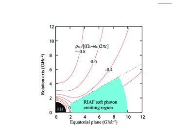
Figure 1.— Side view of an axisymmetric black hole magnetosphere. As a toy model, we assume that the radiatively inefficient accretion flow (RIAF) and the polar funnel is bounded by a cone (dotted line) with colatitude $\theta=60^{\circ}$. The RIAF photons are assumed to be emitted from the cyan shaded region, which is within the colatitude $60^{\circ}<\theta<90^{\circ}$ and the radius $r_{\tiny\rm ISCO}=2.31M<r<r_{\rm out}=10M$ in the Boyer-Lindquist coordinate. The red curves denote the dimensionless Goldreich-Julian (GJ) charge density, where the magnetic field lines are assumed to be radial on the poloidal plane (see also the left panel of fig. 1 in HP16). The red curve labeled with “0” (near $r=2M$) denotes the null-charge surface, around which a gap arises in the polar funnel, $0\leq\theta<60^{\circ}$. Due to frame dragging, the GJ charge density increases inwards near the horizon.

Between the distant static observer (i.e., us) and the LRF, the photon energy changes by the redshift factor,

$$\frac{\omega_{\infty}}{\omega_{\tiny\rm LRF}} = \frac{\mbox{\boldmath$e$}_{(t)}{}^{\infty}\cdot\mbox{\boldmath$k$}}{\mbox{\boldmath$e$}_{(t)}{}^{\tiny\rm LRF}\cdot\mbox{\boldmath$k$}}=\left(\frac{d\tau}{dt}\right)^{\tiny\rm LRF}\frac{-\hbar\omega_{\infty}}{(\mbox{\boldmath$e$}_{(t)}+\beta^{\varphi}\mbox{\boldmath$e$}_{(\varphi)})\cdot\mbox{\boldmath$k$}}$$ (19)

$$= \left(\frac{d\tau}{dt}\right)^{\tiny\rm LRF}\frac{1}{1-\beta^{\varphi}\lambda},$$

where $\lambda\equiv k_{\varphi}/\hbar\omega_{\infty}$ denotes the ratio between the photon angular momentum $k_{\varphi}$ and energy $-k_{t}=\hbar\omega_{\infty}$, both of which are conserved along the ray.

In the coordinate basis, the photon wave vector takes the following components:

$$k_{t}=-\hbar\omega_{\infty} \equiv k_{\alpha}\left[\mbox{\boldmath$e$}_{(t)}\right]^{\alpha}=\left(\frac{d\tau}{dt}\right)^{\tiny\rm LRF}\frac{-\omega_{\tiny\rm LRF}}{1-\beta^{\varphi}\lambda},$$ (20)

$$k_{\varphi}=\lambda\hbar\omega_{\infty} \equiv k_{\alpha}\left[\mbox{\boldmath$e$}_{(\varphi)}\right]^{\alpha},$$ (21)

$$k_{r} \equiv k_{\alpha}\left[\mbox{\boldmath$e$}_{(r)}\right]^{\alpha}=\sqrt{g_{rr}}k_{\hat{r}}{}^{\tiny\rm LRF},$$ (22)

$$k_{\theta} \equiv k_{\alpha}\left[\mbox{\boldmath$e$}_{(\theta)}\right]^{\alpha}=\sqrt{g_{\theta\theta}}k_{\hat{\theta}}{}^{\tiny\rm LRF},$$ (23)

where $\mbox{\boldmath$e$}_{(\mu)}\equiv\partial_{\mu}$. In the next subsection. we use these components, $k_{\mu}$, to ray-trace the photons emitted in the LRF isotropically.

3.2. Light propagation around the BH

As a photon propagates, its energy $-k_{t}$, angular momentum $k_{\varphi}$, and the Carter’s constant (Carter, 1968)

$$Q\equiv(k_{\theta}/k_{t})^{2}+a^{2}\cos^{2}\theta+\lambda^{2}\cot^{2}\theta$$ (24)

are conserved along the ray. Since $Q$ is finite, only the photons having vanishing angular momenta $\lambda$ can propagate toward the rotation axis, $\theta\sim 0$. It is worth noting that most of the soft photons have positive angular momenta, because they are emitted by the rotating plasmas in the RIAF. Figure 1 shows such a situation that soft photons are most efficiently emitted outside the ISCO, thereby having positive angular momenta except when they are emitted into a specific counter-rotational direction in the LRF. As the disc angular momentum increases, the solid angle into which the photons with a fixed range of very small angular momenta (in an absolute value sense) propagate, decreases in the LRF. As a result, only a small portion of the soft photons can propagate to $\theta\sim 0$, leading to a smaller soft photon density in the higher latitudes, $\theta\ll 1$, compared to the middle latitudes, $\theta\sim 1$. It is, therefore, expected that the gap longitudinal width becomes greater near the rotation axis, enhancing gap luminosity (per magnetic flux tube) compared to the middle latitudes. To see this, we must first examine the specific intensity of the RIAF-emitted, soft photon field in the polar funnel, which is defined to be within $\theta<60^{\circ}$ in the present paper.

We tabulate the soft photon specific intensity at each position in the magnetosphere by the ray-tracing method. The dispersion relation $k^{\mu}k_{\mu}=0$ gives the Hamiltonian,

$$H=-k_{t}=-\frac{g_{t\varphi}}{g_{\varphi\varphi}}k_{\varphi}\pm\frac{\rho_{\rm w}}{g_{\varphi\varphi}}\sqrt{k_{\varphi}^{2}+g_{\varphi\varphi}\left(g^{rr}k_{r}^{2}+g^{\theta\theta}k_{\theta}^{2}\right)}.$$ (25)

Thus, the Hamilton-Jacobi relation gives

$$\frac{dr}{dt}=\frac{\partial H}{\partial k_{r}}=\pm\frac{\rho_{\rm w}n_{r}g^{rr}}{\sqrt{\lambda^{2}+g_{\varphi\varphi}(g^{rr}n_{r}^{2}+g^{\theta\theta}n_{\theta}^{2})}},$$ (26)

$$\frac{d\theta}{dt}=\frac{\partial H}{\partial k_{\theta}}=\pm\frac{\rho_{\rm w}n_{\theta}g^{\theta\theta}}{\sqrt{\lambda^{2}+g_{\varphi\varphi}(g^{rr}n_{r}^{2}+g^{\theta\theta}n_{\theta}^{2})}},$$ (27)

$$\frac{dn_{r}}{dt}=\frac{\partial\ln H}{\partial r}=\partial_{r}\left(\frac{g_{t\varphi}}{g_{\varphi\varphi}}\right)\lambda$$

$$\mp \frac{\displaystyle\partial_{r}\left(\frac{\rho_{\rm w}^{2}}{g_{\varphi\varphi}^{2}}\right)\lambda^{2}+\partial_{r}\left(\frac{\rho_{\rm w}^{2}g^{rr}}{g_{\varphi\varphi}}\right)n_{r}^{2}+\partial_{r}\left(\frac{\rho_{\rm w}^{2}g^{\theta\theta}}{g_{\varphi\varphi}}\right)n_{\theta}^{2}}{\displaystyle\frac{\rho_{\rm w}}{g_{\varphi\varphi}}\sqrt{\lambda^{2}+g_{\varphi\varphi}(g^{rr}n_{r}^{2}+g^{\theta\theta}n_{\theta}^{2})}},$$

$$\frac{dn_{\theta}}{dt}=\frac{\partial\ln H}{\partial\theta}=\partial_{\theta}\left(\frac{g_{t\varphi}}{g_{\varphi\varphi}}\right)\lambda$$

$$\mp \frac{\displaystyle\partial_{\theta}\left(\frac{\rho_{\rm w}^{2}}{g_{\varphi\varphi}^{2}}\right)\lambda^{2}+\partial_{\theta}\left(\frac{\rho_{\rm w}^{2}g^{rr}}{g_{\varphi\varphi}}\right)n_{r}^{2}+\partial_{\theta}\left(\frac{\rho_{\rm w}^{2}g^{\theta\theta}}{g_{\varphi\varphi}}\right)n_{\theta}^{2}}{\displaystyle\frac{\rho_{\rm w}}{g_{\varphi\varphi}}\sqrt{\lambda^{2}+g_{\varphi\varphi}(g^{rr}n_{r}^{2}+g^{\theta\theta}n_{\theta}^{2})}},$$

where the wave numbers are normalized by the conserved wave energy such that $n_{r}\equiv k_{r}/(\hbar\omega_{\infty})$ and $n_{\theta}\equiv k_{\theta}/(\hbar\omega_{\infty})$. Note that the time coordinate $t$ for a distant static observer plays the role of an affine parameter because of the definition of $H$. The initial values of $n_{r}$ and $n_{\theta}$ are calculated by equations (13), (15), (16), (19), (22), and (23).

We integrate equations (26)–(LABEL:eq:HJ_kth) along the individual rays of the RIAF-emitted photons, and tabulate the specific intensity, $I_{\omega}$, at each position on the poloidal plane in the static frame. Note that the static limit touches the horizon at $\theta=0$, that the inward positronic flux dominates the outward electrons’ near the horizon, and that these positrons could only tail-on collide with the inward-unidirectional photons near the horizon. Thus, this treatment, which tabulates $I_{\omega}$ in the static frame, incurs only negligible errors, although the static frame becomes space-like near the horizon in the middle latitudes.

3.3. The zero-angular-momentum observer (ZAMO)

In this paper, we compute the collision frequencies of two-photon pair creation and inverse-Compton scatterings (ICS) in the frame of a zero-angular-momentum observer (ZAMO), which rotates with the same angular frequency as the space-time dragging frequency, $\omega_{\rm drag}\equiv-g_{t\varphi}/g_{\varphi\varphi}$. Putting $\beta^{\varphi}=\omega_{\rm drag}$ in equations (A2), we thus obtain the lapse

$$\frac{d\tau}{dt}=\alpha\equiv\frac{\rho_{\rm w}}{\sqrt{g_{\varphi\varphi}}}.$$ (30)

The tetrad of ZAMO is obtained from equations (A9)–(A12) and becomes

$$\mbox{\boldmath$e$}_{(\hat{t})}{}^{\tiny\rm ZAMO}=\alpha^{-1}(\mbox{\boldmath$e$}_{(t)}+\omega_{\rm drag}\mbox{\boldmath$e$}_{(\varphi)}),$$ (31)

$$\mbox{\boldmath$e$}_{(\hat{r})}{}^{\tiny\rm ZAMO}=\sqrt{\frac{\Delta}{\Sigma}}\mbox{\boldmath$e$}_{(r)},$$ (32)

$$\mbox{\boldmath$e$}_{(\hat{\theta})}{}^{\tiny\rm ZAMO}=\frac{1}{\sqrt{\Sigma}}\mbox{\boldmath$e$}_{(\theta)},$$ (33)

$$\mbox{\boldmath$e$}_{(\hat{\varphi})}{}^{\tiny\rm ZAMO}=\frac{1}{\sqrt{g_{\varphi\varphi}}}\mbox{\boldmath$e$}_{(\varphi)}.$$ (34)

Between the distant static observer and ZAMO, the photon energy changes by the redshift factor,

$$\frac{\omega_{\infty}}{\omega_{\tiny\rm ZAMO}}=\frac{\mbox{\boldmath$e$}_{(t)}{}^{\infty}\cdot\mbox{\boldmath$k$}}{\mbox{\boldmath$e$}_{(t)}{}^{\tiny\rm ZAMO}\cdot\mbox{\boldmath$k$}}=\frac{\alpha}{1-\beta^{\varphi}\lambda}.$$ (35)

Combining equations (19) and (35), we find that the photon energy changes from the LRF to ZAMO by the factor

$$g_{\rm s}\equiv\frac{\omega_{\tiny\rm ZAMO}}{\omega_{\tiny\rm LRF}}=\alpha^{-1}\left(\frac{d\tau}{dt}\right)^{\tiny\rm LRF}\frac{1-\omega_{\rm drag}\lambda}{1-\Omega_{\rm K}\lambda}.$$ (36)

3.4. Angular distribution of RIAF soft photons in ZAMO

Emitting $200\times 128$ test photons isotropically in LRF from $14\times 14$ positions homogeneously on the poloidal plane (§ 3.1), we construct the specific intensity, $I_{\omega}$, at each position ($r$,$\theta$) in each directional bin in the static frame. To compute the photon propagation direction in ZAMO, we could use the solved $n_{r}$, $n_{\theta}$, and $n_{\varphi}$ and convert the momentum from the static frame to ZAMO. It is, however, more straightforward to use the photon wave vector, $k_{\hat{i}}$, measured in ZAMO. To compute $k_{\hat{i}}$, we set $d\tau/dt=\alpha$ and $\beta^{\varphi}=\omega_{\rm drag}$ in equations (A13)–(A16) (or equivalently, eqs. [A9]–[A12]) to obtain

$$k_{\hat{t}}{}^{\tiny\rm ZAMO} = -\omega_{\tiny\rm ZAMO},$$ (37)

$$k_{\hat{r}}{}^{\tiny\rm ZAMO} = b\sqrt{g_{rr}}\frac{dr}{dt},$$ (38)

$$k_{\hat{\theta}}{}^{\tiny\rm ZAMO} = b\sqrt{g_{\theta\theta}}\frac{d\theta}{dt},$$ (39)

$$k_{\hat{\varphi}}{}^{\tiny\rm ZAMO} = b\sqrt{g_{\varphi\varphi}}\left(\frac{d\varphi}{dt}-\omega_{\rm drag}\right),$$ (40)

where the dispersion relation $k^{\mu}k_{\mu}=0$, or equivalently,

$$(k_{\hat{r}}{}^{\tiny\rm ZAMO})^{2}+(k_{\hat{\theta}}{}^{\tiny\rm ZAMO})^{2}+(k_{\hat{\varphi}}{}^{\tiny\rm ZAMO})^{2}=\omega_{\tiny\rm ZAMO}^{2}.$$ (41)

gives

$$b=\frac{\omega_{\rm ZAMO}}{\displaystyle\sqrt{g_{rr}\left(\frac{dr}{dt}\right)^{2}+g_{\theta\theta}\left(\frac{d\theta}{dt}\right)^{2}+g_{\varphi\varphi}\left(\frac{d\varphi}{dt}-\omega_{\rm drag}\right)^{2}}}.$$ (42)

In the Boyer-Lindquist coordinates, the ray-tracing result automatically gives ($dr/dt$,$d\theta/dt$,$d\varphi/dt$) in the static frame. Then we can readily convert it into the ZAMO-measured propagation direction, ($\theta_{\gamma}{}^{\tiny\rm ZAMO}$, $\varphi_{\gamma}{}^{\tiny\rm ZAMO}$), using equations (38)–(40), where

$$k_{\hat{r}}{}^{\tiny\rm ZAMO} = \omega_{\tiny\rm ZAMO}\cos\theta_{\gamma}{}^{\tiny\rm ZAMO},$$ (43)

$$k_{\hat{\theta}}{}^{\tiny\rm ZAMO} = \omega_{\tiny\rm ZAMO}\sin\theta_{\gamma}{}^{\tiny\rm ZAMO}\cos\varphi_{\gamma}{}^{\tiny\rm ZAMO},$$ (44)

$$k_{\hat{\varphi}}{}^{\tiny\rm ZAMO} = \omega_{\tiny\rm ZAMO}\sin\theta_{\gamma}{}^{\tiny\rm ZAMO}\sin\varphi_{\gamma}{}^{\tiny\rm ZAMO}.$$ (45)

Equation (43) gives the photon’s propagation angle in ZAMO with respect to the radial outward direction, $\theta_{\gamma}{}^{\tiny\rm ZAMO}=\cos^{-1}(k_{\hat{r}}{}^{\tiny\rm ZAMO}/\omega_{\tiny\rm ZAMO})$. Equation (44) or (45) gives the azimuthal propagation direction, $\varphi_{\gamma}{}^{\tiny\rm ZAMO}$, measured around the local radial direction.

We convert the specific intensity $I_{\omega}$ tabulated in the static frame (§ 3.2) into the ZAMO-measured value, by using the invariance of $I_{\omega}\omega^{-3}$ under general coordinate transformation. Integrating this ZAMO-measured specific intensity over the propagation solid angle in each directional bin at each point in ZAMO, we obtain the soft photon flux at each point in each direction. Finally, we use this flux to compute the ICS optical depth and the photon-photon collision optical depth in ZAMO (see also the description around eq. (38) of Li et al., 2008).

When we compute the photon-photon absorption and ICS optical depths, we need the soft-photon differential number flux, $dF_{\rm s}/dE_{\rm s}$ (photons per unit time per unit area per energy) at each point and in each direction. In (Hirotani & Pu, 2016, hereafter HP16) and H16, we adopted the analytical solution (Mahadevan, 1997) of the advection-dominated-accretion flow (ADAF) as an RIAF, and computed $dF_{\rm s}/dE_{\rm s}$ assuming that all the soft photons were emitted at $r=0$ with the spatially integrated ADAF spectrum $dL/dE_{\rm s}$ (luminosity per photon energy), and propagated radially to radius $r$ in a flat spacetime. This outwardly unidirectional photon differential number flux, $(dL/dE_{\rm s})/(4\pi r^{2}E_{\rm s})$ (photons per unit time per unit area per energy), is further divided by the number of photon-propagation-directional bins at each point, so that we may impose a homogeneous ADAF soft photon field. What is more, in HP16 and H16, we assumed that this isotropic photon differential number flux at $r<6M$ took the same value as that at $r=6M$. Denoting this Newtonian isotropic photon differential number flux at $r=6M$ as $(dF_{\rm s}/dE_{\rm s})_{0}$, we can express $dF_{\rm s}/dE_{\rm s}=f_{\rm riaf}(dF_{\rm s}/dE_{\rm s})_{0}$, where $f_{\rm riaf}=\min[1,(6M/r)^{2}]$. which were used in equations (31), (38), and (40) of H16.

In the present paper, we instead compute $dF_{\rm s}/dE_{\rm s}$ in ZAMO by the method described above. Then the flux correction factor is tabulated at each position by $f_{\rm riaf}(r,\theta,\cos\theta_{\gamma}{}^{\tiny\rm ZAMO})\equiv(dF_{\rm s}/dE_{\rm s})/(dF_{\rm s}/dE_{\rm s})_{0}$. When computing the photon-photon absorption and ICS optical depths, we multiply this $f_{\rm riaf}$ in the integrant of equations (38) and (40) of HP16. Note that equation (31) of HP16 is no longer used in the present paper, because we abandon the mono-energetic approximation and instead solve the Lorentz-factor dependence of the lepton distribution functions.

In figure 2, we present the flux correction factor, $f_{\rm riaf}$, assuming $a=0.9M$. The four panels show its values along the four discrete radial poloidal magnetic field lines, $\theta=0^{\circ}$, $15^{\circ}$, $30^{\circ}$, and $45^{\circ}$ from the rotation axis. The five curves in each panel represent the $f_{\rm riaf}$ measured at the five Boyer-Lindquist radial coordinates, $r=2M$, $4M$, $6M$, $15M$, and $30M$ The abscissa denotes the photon propagation direction with respect to the local radial direction: $\cos\theta_{\gamma}{}^{\tiny\rm ZAMO}=-1$ corresponds to a radially inward propagation, while $\cos\theta_{\gamma}{}^{\tiny\rm ZAMO}=1$ a radially outward one. In our previous works (HP16 and H16), $f_{\rm riaf}=\min[1,(6M/r)^{2}]$ was assumed in any directions $-1<\cos\theta_{\gamma}{}^{\tiny\rm ZAMO}<1$ at all the colatitude $\theta$ from the rotation axis.

Comparing the four panels, we find that the photon intensity decreases with decreasing $\theta$, because most of the photons have positive $\lambda$ and hence difficult to approach the rotation axis, $\theta=0^{\circ}$. The solid curves (at $r=2M$) in each panel show that the radiation field becomes predominantly inward near the horizon, owing to the causality, where the horizon is located at $r_{\rm H}=1.435M$ in the present case of $a=0.9M$. However, at larger $r$, the radiation field becomes outwardly unidirectional and its flux decreases by $r^{-2}$ law, as the blue (at $r=15M$) and cyan (at $r=30M$) curves indicate. This is because the RIAF photons are emitted only within $r_{\rm out}=10M$ in the present consideration.

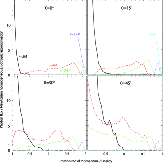
Figure 2.— RIAF photon flux correction factor, $f_{\rm riaf}$, as a function of the propagation direction, $\theta_{\gamma}{}^{\tiny\rm ZAMO}$, with respect to the radially outward direction, at several discrete radial and latitudinal positions. A large BH spin, $a=0.9M$, is assumed. In the abscissa, $\cos\theta_{\gamma}{}^{\tiny\rm ZAMO}=-1$ corresponds to the radially inward propagation, while $\cos\theta_{\gamma}{}^{\tiny\rm ZAMO}=1$ does radially outward propagation. The black solid, red dashed, green dash-dotted, blue dotted, and cyan dash-dot-dot-dotted curves show $f_{\rm riaf}$ at $r=2M$, $4M$, $6M$, $15M$, and $30M$, respectively.

4. Magnetospheric lepton accelerator near the horizon

Being illuminated by the soft photon field described in § 3, a stationary lepton accelerator can be sustained close to the horizon (HP16). In this section, we formulate the electrodynamics of such a stationary BH gap, extending the method described in H16. In the same way as § 3, throughout this paper, we assume an aligned rotator in the sense that the magnetic axis coincides with the rotational axis of the BH, and consider only the ‘axisymmetric’ solutions in the sense that any quantity does not depend on $\varphi-\Omega_{\rm F}t$.

4.1. Magnetic field structure

As demonstrated in H16, a stationary BH gap arises around the null surface that is formed by the frame-dragging effect near the horizon. Accordingly, the gap electrodynamics is essentially governed by the frame-dragging rather than the magnetic field configurations. We therefore assume a radial magnetic field on the poloidal plane, $\Psi=\Psi(\theta)$.

Since we do not know the toroidal component of the magnetic field, we cannot constrain the angular momentum of the $\gamma$-ray photons emitted from the gap. For simplicity, we thus assume that the gap-emitted photons have vanishing angular momenta. Under this assumption, gap-emitted $\gamma$-rays propagate radially on the poloidal plane and collide with the RIAF-emitted soft photons in ZAMO with the angle $\theta_{\rm c}=\theta_{\gamma}{}^{\tiny\rm ZAMO}$ for outward $\gamma$-rays, and with the angle $\pi-\theta_{\gamma}{}^{\tiny\rm ZAMO}$ for inward $\gamma$-rays. To compute the rate of ICS, we assume that outwardly migrating electrons collide with the soft photons with the same angle $\theta_{\rm c}$ as the outward $\gamma$-rays, and that the inwardly migrating positrons does with the same angle $\pi-\theta_{\rm c}$ as the inward $\gamma$-rays.

As for the curvature process, we parameterize the curvature radius, $R_{\rm c}$, of the particles, instead of constraining it from their 3-D motion. It is, indeed, the IC-emitted, VHE photons (not the curvature-emitted, HE photons) that materialize as pairs colliding with the RIAF submillimeter photons. Thus, the actual value of $R_{\rm c}$ does not affect the gap electrodynamics. We thus adopt $R_{\rm c}=M$ in the present paper, leaving the toroidal magnetic field component, $B_{\varphi}$, unconstrained.

4.2. Gap electrodynamics

In the same way as HP16, we solve the stationary gap solution from the set of the Poisson equation for $\Phi$, the equations of motion for the created leptons, and the radiative transfer equation for the emitted photons.

4.2.1 Poisson equation

To solve the radial dependence of $\Phi$ in the Poisson equation (5), we introduce the following dimensionless tortoise coordinate, $\eta_{\ast}$,

$$\frac{d\eta_{\ast}}{dr}=\frac{r^{2}+a^{2}}{\Delta}\frac{1}{M}.$$ (46)

In this coordinate, the horizon corresponds to the negative infinity, $\eta_{\ast}=-\infty$. It is convenient to set $\eta_{\ast}=rM^{-1}$ at some large enough radius $r=r_{3}$. In this paper, we put $r_{3}=25M$ (i.e., $\eta_{\ast}=25$ at $r=25M$), the actual value of which never affects the results in any ways.

Since the gap is located near the horizon, we take the limit $\Delta\ll M^{2}$. Assuming that $\Phi$ does not depend on $\varphi-\Omega_{\rm F}t$, $\Phi=\Phi(r,\theta)$ is solved from the two-dimensional Poisson equation,

$$-\left(\frac{r^{2}+a^{2}}{\Delta}\right)^{2}\frac{\partial^{2}\tilde{\Phi}}{\partial\eta_{\ast}{}^{2}}+\frac{2(r-M)(r^{2}+a^{2})}{\Delta^{2}/M}\frac{\partial\tilde{\Phi}}{\partial\eta_{\ast}}$$

$$-\frac{M^{2}}{\Delta}\frac{\Sigma}{\sin\theta}\frac{\partial}{\partial\theta}\left(\frac{\sin\theta}{\Sigma}\frac{\partial\tilde{\Phi}}{\partial\theta}\right)$$

$$=\left(\frac{\Sigma}{r^{2}+a^{2}}\right)^{2}\left[\int(n_{+}-n_{-})d\gamma-n_{\rm GJ}\right],$$ (47)

where

$$\tilde{\Phi}(\eta_{\ast})\equiv\frac{1}{\Omega_{\rm F}BM^{2}}\Phi(r)$$ (48)

denotes the dimensionless non-corotational potential. Dimensionless lepton distribution functions per magnetic flux tube are defined by

$$n_{\pm}\equiv\frac{2\pi ce}{\Omega_{\rm F}B}N_{\pm}(r,\theta,\gamma),$$ (49)

where $N_{+}$ and $N_{-}$ designate the distribution functions of the leptons, respectively; $\gamma$ refers to the lepton’s Lorentz factor. Dimensionless GJ charge density per magnetic flux tube is defined by

$$n_{\rm GJ}\equiv\frac{2\pi c}{\Omega_{\rm F}B}\rho_{{\rm GJ}}.$$ (50)

If the real charge density, $\int(n_{+}-n_{-})d\gamma$, deviates from $n_{\rm GJ}$ in some region, electric field inevitably appears along the magnetic field lines around that region.

For a radial poloidal magnetic field, $\Psi=\Psi(\theta)$, we can compute the acceleration electric field by

$$E_{\parallel}\equiv-\frac{\partial\Phi}{\partial r}=-M\Omega_{\rm F}B\frac{r^{2}+a^{2}}{\Delta}\frac{\partial\tilde{\Phi}}{\partial\eta_{\ast}}.$$ (51)

Without loss of any generality, we can assume $F_{\theta\varphi}>0$ (i.e., outward magnetic field direction) in the northern hemisphere. In this case, a negative $E_{\parallel}$ arises in the gap, which is consistent with the direction of the global current flow pattern.

4.2.2 Particle Boltzmann equations

We follow the argument presented in § 3 of Hirotani (2013) on pulsar outer gap model. Imposing a stationary condition, $\partial/\partial t+\Omega_{\rm F}\partial/\partial\phi=0,$ we obtain the following Boltzmann equations,

$$c\cos\chi\frac{\partial n_{\pm}}{\partial s}+\dot{p}\frac{\partial n_{\pm}}{\partial p}=\alpha(S_{{\rm IC},\pm}+S_{{\rm p},\pm}),$$ (52)

along each radial magnetic field line on the poloidal plane, where $c$ is recovered, the upper and lower signs correspond to the positrons (with charge $q=+e$) and electrons ($q=-e$), respectively, and $p\equiv|\mbox{\boldmath$p$}|=m_{\rm e}c\sqrt{\gamma^{2}-1}$. Since pair annihilation and magnetic pair creation are negligible in BH magnetospheres under low accretion rate (and hence under weak magnetic field strength), the right-hand side contains the collision terms due to ICS and photon-photon pair creation. The left-hand side is in $dt$ basis, where $t$ denotes the proper time of a distant static observer. Thus, the lapse $\alpha$ is multiplied in the right-hand side, because both $S_{\rm IC}$ and $S_{\rm p}$ are evaluated in ZAMO. On the poloidal plane, equation (1) gives $ds=\sqrt{g_{rr}dr^{2}+g_{\theta\theta}d\theta^{2}}$. However, as described in § 4.1, we neglect meridional propagation of the gap-emitted photons; thus, we obtain $ds=dr$.

When particles emit photons via synchro-curvature process, the energy loss ($\sim$ GeV) is small compared to the particle energy ($\sim 10$ TeV); thus, it is convenient to include the back reaction of the synchro-curvature emission as a friction term in the left-hand side. In this case, the characteristics of equation in the phase space ($s$,$p$) is given by

$$\dot{p}\equiv qE_{\parallel}\cos\chi-\frac{P_{\rm SC}}{c},$$ (53)

where the pitch angle is assumed to be $\chi=0$ for outwardly moving positrons, and $\chi=\pi$ for inwardly moving electrons. In this zero-pitch-angle approximation, the synchro-curvature radiation force (Cheng & Zhang, 1996; Zhang & Cheng, 1997), $P_{\rm SC}/c$, is simply given by the pure curvature formula (e.g., Harding, 1981), $P_{\rm SC}/c=2e^{2}\gamma^{4}/(3R_{\rm c}{}^{2})$. The particle position $s$ is related with time $t$ by $\dot{s}=ds/dt=c\cos\chi$.

In equation (52), the IC collision terms are expressed as

$$S_{\rm IC} \equiv -\int_{\epsilon_{\gamma}<\gamma}d\epsilon_{\gamma}\eta_{\rm IC}^{\gamma}(\epsilon_{\gamma},\gamma,\mu_{\pm})n_{\pm}$$ (54)

$$+ \int_{\gamma_{i}>\gamma}d\gamma_{i}\eta_{\rm IC}^{\rm e}(\gamma_{i},\gamma,\mu_{\pm})n_{\pm},$$

where the IC redistribution function is defined by

$$\eta_{\rm IC}^{\gamma}\equiv(1-\beta\mu_{\pm})\int_{E_{\rm min}}^{E_{\rm max}}dE_{\rm s}\frac{dF_{\rm s}}{dE_{\rm s}}\frac{d\epsilon_{\gamma}^{\ast}}{d\epsilon_{\gamma}}\int_{-1}^{1}d\Omega_{\gamma}^{\ast}\frac{d\sigma_{\rm KN}^{\ast}}{d\epsilon_{\gamma}^{\ast}d\Omega_{\gamma}^{\ast}},$$ (55)

$m_{\rm e}c^{2}\epsilon_{\gamma}$ denotes the upscattered $\gamma$-ray energy. The asterisk denotes that the quantity evaluated in the electron rest frame and $d\sigma_{\rm KN}^{\ast}/d\epsilon_{\gamma}^{\ast}d\Omega_{\gamma}^{\ast}$ denotes the Klein-Nishina differential cross section. Energy conservation gives

$$\eta_{\rm IC}^{\rm e}(\gamma_{i},\gamma,\mu_{\pm})=\eta_{\rm IC}^{\gamma}(\gamma_{i}-\gamma,\gamma_{i},\mu_{\pm}),$$ (56)

where $\gamma_{i}$ denotes the Lorentz factor before collision and $\mu_{+}$ (or $\mu_{-}$) does the cosine of the collision angle with the soft photon for outwardly moving electrons (or inwardly moving positrons). For more details, see § 3.2.2 of Hirotani et al. (2003). The effect of inhomogeneous and anisotropic RIAF photon field is included in the differential soft photon flux, $dF_{\rm s}/dE_{\rm s}$, through the correction factor $f_{\rm riaf}$ (see the last part of § 3.4). That is, we put $dF_{\rm s}/dE_{\rm s}=f_{\rm riaf}\cdot(dF_{\rm s}/dE_{\rm s})_{0}$.

The photon-photon pair creation term becomes

$$S_{\rm p}\equiv\int d\nu_{\gamma}\alpha_{\gamma\gamma}\frac{2\pi e}{\Omega B}\int\frac{I_{\omega}}{\hbar\omega}d\Omega,$$ (57)

where

$$\alpha_{\gamma\gamma}=(1-\mu_{\pm})\int_{E_{\rm th}}^{\infty}dE_{\rm s}\frac{dF_{\rm s}}{dE_{\rm s}}\frac{d\sigma_{\gamma\gamma}}{d\gamma},$$ (58)

The $\gamma$-ray specific intensity $I_{\omega}$ is integrated over the $\gamma$-ray propagation solid angle $\Omega_{\gamma}$. For details, see § 3.2.2 of (Hirotani et al., 2003). Note that $dF_{\rm s}/dE_{\rm s}$ in both $\eta_{\rm IC}^{\gamma}$ and $\alpha_{\gamma\gamma}$ is evaluated in ZAMO as described in § 3.4.

Let us consider how the created leptons affect the right-hand side of equation (47). Because $E_{\parallel}$ is negative, electrons are accelerated outwards, while positrons inwards. As s result, charge density, $\int(n_{+}-n_{-})d\gamma$, becomes negative (or positive) at the outer (or inner) boundary. In a stationary gap, $E_{\parallel}$ should not change sign in it. In a vacuum gap ($n_{+}=n_{-}=0$), a positive (or a negative) $-n_{\rm GJ}$ near the outer (or inner) boundary makes $\partial_{r}E_{\parallel}>0$ (or $\partial_{r}E_{\parallel}<0$), thereby closing the gap. In a non-vacuum gap, the right-hand side of equation (47) should become positive (or negative) near the outer (or inner) boundary so that the gap may be closed. Therefore, $|\int(n_{+}-n_{-})d\gamma|$ should not exceed $|n_{\rm GJ}|$ at either boundary. At the outer boundary, for instance, the dimensionless lepton distribution functions satisfy

$$(n_{+}-n_{-})|_{r=r_{2}}=-n_{-}(r_{2},\gamma)=jn_{\rm GJ}(r_{2})\delta(\gamma-\gamma_{0}),$$ (59)

where $\gamma_{0}$ denotes the Lorentz factor of the injected leptons, and does not affect the results unless it becomes comparable to the typical Lorentz factors in the gap. The dimensionless electric current density, $j$, should be in the range, $0\leq j\leq 1$, so that the gap solution may be stationary. If $j=1$, there is no surface charge at the outer boundary. However, if $j<1$, the surface charge results in a jump of $\partial_{r}E_{\parallel}$ at the outer boundary. That is, the parameter $j$ specifies the strength of $\partial_{r}E_{\parallel}$ at the outer boundary. Thus, the inner boundary position, $r=r_{1}$, is determined as a free boundary problem by this additional constraint, $j$. The outer boundary position, $r=r_{2}$, or equivalently the gap width $w=r_{2}-r_{1}$, is constrained by the gap closure condition (§ 4.2.5).

It is noteworthy that the charge conservation ensures that the dimensionless current density (per magnetic flux tube), $J_{\rm e}\equiv\int(-n_{+}-n_{-})d\gamma$ conserves along the flowline. At the outer boundary, we obtain

$$J_{\rm e}=-\int n_{-}(r_{2},\gamma)d\gamma=jn_{\rm GJ}(r_{2}).$$ (60)

Thus, $j$ specifies not only $\partial_{r}E_{\parallel}$ at the outer boundary, but also the conserved current density, $J_{\rm e}$.

In general, under a given electro-motive force exerted in the ergosphere, $J_{\rm e}$ should be constrained by the global current flow pattern, which includes an electric load at the large distances where the force-free approximation breaks down and the trans-magnetic-field current gives rise to the outward acceleration of charged particles by Lorentz forces (thereby converting the Poynting flux into particle kinetic energies). However, we will not go deep into the determination of $J_{\rm e}$ in this paper, because we are concerned with the acceleration processes near the horizon, not the global current closure issue. Note that $w$ (or $r_{2}$) is essentially determined by $\dot{m}$; thus, $j$ and $\dot{m}$ give the actual current density $(\Omega_{\rm F}B/2\pi)J_{\rm e}$, where $B$ should be evaluated at each position. On these grounds, instead of determining $J_{\rm e}$ by a global requirement, we treat $j$ as a free parameter in the present paper. To consider a stationary gap solution, we restrict the range of $j$ as $0\leq j\leq 1$ (see the end of § 4.2.2 of H16).

4.2.3 Radiative transfer equation

In the same manner as H16, we assume that all photons are emitted with vanishing angular momenta and hence propagate on a constant-$\theta$ cone. Under this assumption of radial propagation, we obtain the radiative transfer equation (Hirotani, 2013),

$$\frac{dI_{\omega}}{dl}=-\alpha_{\omega}I_{\omega}+j_{\omega},$$ (61)

where $dl=\sqrt{g_{rr}}dr$ refers to the distance interval along the ray in ZAMO, $\alpha_{\omega}$ and $j_{\omega}$ the absorption and emission coefficients evaluated in ZAMO, respectively. We consider only photon-photon collisions for absorption, pure curvature and IC processes for primary lepton emissions, and synchrotron and IC processes for the emissions by secondary and higher-generation pairs. For more details of the computation of absorption and emission, see §§ 4.2 and 4.3 of HP16 and § 5.1.5 of H16. (Regretfully, there was a typo in an equation after eq. [29] of H16. The local photon energy, $h\nu^{\prime}$, is related to $h\nu$, by $h\nu^{\prime}=\dot{t}(h\nu-m\cdot d\varphi/dt)$; that is, the sign should be negative, not positive.)

Some portions of the photons are emitted above 10 TeV via IC process. A significant fraction of such hard $\gamma$-rays are absorbed, colliding with the RIAF soft photons. If such collisions take place within the gap, the created electrons and positrons polarize to be accelerated in opposite directions, becoming the primary leptons. If the collisions take place outside the gap, the created, secondary pairs migrate along the magnetic filed lines to emit photons via IC and synchrotron processes. Some of such secondary IC photons are absorbed again to materialize as tertiary pairs, which emit tertiary photons via synchrotron and IC processes, eventually cascading into higher generations.

4.2.4 Boundary conditions

In this subsection, we describe the boundary conditions imposed on the three basic equations, Eqs. (47), (52), and (61), one by one.

First, let us consider the elliptic type second-order partial differential equation (5). In the 2-D poloidal plane, we assume a reflection symmetry with respect to the magnetic axis. Thus, we put $\partial_{\theta}\tilde{\Phi}=0$ at $\theta=0$. We assume that the polar funnel is bounded at a fixed colatitude, $\theta=\theta_{\rm max}$ and impose that this lower-latitude boundary is equi-potential and put $\tilde{\Phi}=0$ at $\theta=\theta_{\rm max}$.

Both the outer and inner boundaries are treated as free boundaries. At both boundaries, $E_{\parallel}$ vanishes. To determine the positions of the two boundaries, we impose the following two conditions: The value of $j$ along each magnetic field line, and the gap closure condition (to be described in § 4.2.5). For simplicity, we assume that $j$ is constant on all the field lines. The closure condition constrains the gap width, $w=r_{2}-r_{1}$, and $j$ does $\partial_{r}E_{\parallel}=-\partial_{r}{}^{2}\Phi$ at the outer boundary. This additional condition, $\partial_{r}E_{\parallel}$ constrains the the inner boundary position $r=r_{1}$, and hence the outer boundary position, $r_{2}=w+r_{1}$.

Second, consider the hyperbolic type first-order partial differential equations (52). We assume that neither electrons nor positrons are injected across either the outer or the inner boundaries.

Third, consider the first-order ordinary differential equation (61). We assume that photons are not injected across neither the outer nor the inner boundaries.

4.2.5 Gap closure condition

The set of Poisson and Boltzmann equations are solved under the boundary conditions mentioned just above. In H16, we adopted the mono-energetic approximation to the particle distribution functions. However, in this paper, we explicitly solve their $\gamma$ dependence at each position $s$. Accordingly, we compute the multiplicity (eq. [41] of HP16) of primary electrons, ${\cal M}_{\rm out}$, and that of primary positrons, ${\cal M}_{\rm in}$, summing up all the created pairs by individual test particles and dividing the result by the number of test particles. With this modification, we apply the same closure condition that a stationary gap may be sustained, ${\cal M}_{\rm in}{\cal M}_{\rm out}=1$.

5. Gap solutions around super-massive black holes

In this paper, we apply the method described in the foregoing section to SMBHs. Unless explicitly mentioned, we adopt $a=0.90M$, $\Omega_{\rm F}=0.50\omega_{\rm H}$, $r_{\rm out}=10M$, $j=0.7$, and $R_{\rm c}=M$. To solve the Poisson equation (47), we set the meridional boundary at $\theta=\theta_{\rm max}=60^{\circ}$.

5.1. The case of billion solar mass BHs

Let us first examine the gap solutions when the BH mass is $M=10^{9}M_{\odot}$.

5.1.1 Acceleration electric field on the poloidal plane

We begin with presenting the distribution of $E_{\parallel}$ on the poloidal plane. In figure 3, we plot $E_{\parallel}$ (in statvolt ${\rm cm}^{-1}$) as a function of the dimensionless tortoise coordinate, $\eta_{\ast}=r_{\ast}/M$, and the magnetic colatitude, $\theta$ (in degrees), for the dimensionless accretion of $\dot{m}=1.77\times 10^{-5}$. Near the lower-latitude boundary, $\theta=60^{\circ}$, a small $E_{\parallel}$ extends in an extended gap width along the poloidal magnetic field line. However, near the rotation axis, $\theta=0^{\circ}$, much stronger $E_{\parallel}$ arises, because this region is located away from the meridional boundary at $\theta=60^{\circ}$. Since the equatorial region is assumed to be grounded to the near-horizon region by a dense accreting plasma, $E_{\parallel}$ vanishes in $\theta>60^{\circ}$. The selection of $60^{\circ}$ is, indeed, arbitrary. For example, if the equatorial disk is geometrically thin within $89^{\circ}<\theta<91^{\circ}$, figure 3 will be stretched horizontally to $\theta=89^{\circ}$.

In figure 4, we also plot $E_{\parallel}$ at six discrete colatitudes, $\theta=0^{\circ}$, $15^{\circ}$, $30^{\circ}$, $37.5^{\circ}$, and $45^{\circ}$. It follows that the $E_{\parallel}(\eta_{\ast})$ distribution little changes in the polar region within $\theta\leq 15^{\circ}$. It is noteworthy that in H16 $E_{\parallel}(\eta_{\ast})$ distribution little changes within $\theta<38^{\circ}$. The reason of this polar concentration in the present work is that the the RIAF-emitted photons do not efficiently illuminate the polar regions, $\theta\leq 15^{\circ}$, owing to their preferentially positive angular momenta.

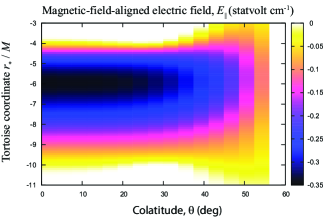
Figure 3.— Acceleration electric field (statvolt ${\rm cm}^{-1}$) on the poloidal plane. The abscissa denotes the magnetic colatitudes, $\theta$, in degrees, where $0$ (i.e., the ordinate) corresponds to the magnetic axis. The ordinate denotes the dimensionless tortoise coordinate, where $-\infty$ corresponds to the event horizon. The gap is solved for a black hole with $M=10^{9}M_{\odot}$ and $a_{\ast}=0.9$. Dimensionless accretion rate is chosen to be $\dot{m}=1.77\times 10^{-5}$.

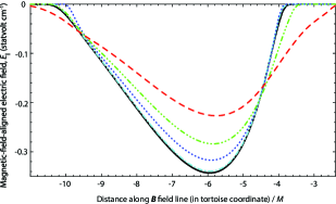
Figure 4.— Acceleration electric field at five discrete colatitudes, $\theta$, as a function of the dimensionless tortoise coordinate, $\eta_{\ast}$, for $\dot{m}=1.77\times 10^{-5}$. The black solid, cyan dash-dotted, blue dotted, green dash-dot-dot-dotted, and red dashed, curves denote the $E_{\parallel}$ at $\theta=0^{\circ}$, $15^{\circ}$, $30^{\circ}$, $37.5^{\circ}$, and $45^{\circ}$, respectively.

5.1.2 Gap emission versus colatitudes

We next compare the $\gamma$-ray spectra of a BH gap emission as a function of the colatitude, $\theta$. In figure 5, we compare the SEDs at the same five discrete $\theta$’s as in figure 4. It follows that the gap emission becomes most luminous if we observe the gap nearly face-on with a viewing angle $\theta\leq 15^{\circ}$. Although the $E_{\parallel}(s)$ distribution little changes between $\theta=0^{\circ}$ and $15^{\circ}$, the reduced soft photon density at $\theta\approx 0^{\circ}$ (particularly near the gap center, $r\approx 2M$; fig. 2) results in a smaller IC drag force and hence greater electron Lorentz factors near the rotation axis. Thus, the IC spectrum becomes harder at $\theta=0^{\circ}$ than $\theta=15^{\circ}$; this point was not included in HP16 or H16, both of which adopted a homogeneous RIAF photon density in the funnel. It should be noted that the angular distribution of the gap emission is beamed into a smaller solid angle, compared to figure 4 of H16. This is due to the small RIAF photon density near the rotation axis.

The conclusion that the gap emission gets stronger and harder near the rotation axis, $\theta<15^{\circ}$, is unchanged if we adopt different BH masses or spins. Therefore, in what follows, we adopt $\theta=0$ as the representative colatitude to estimate the greatest and hardest $\gamma$-ray flux of BH gaps.

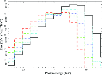
Figure 5.— Spectral energy distribution (SED) of the emission from a black hole (BH) gap at five discrete colatitudes, $\theta$, at a distance of 10 Mpc. The gap is solved for a black hole with $M=10^{9}M_{\odot}$ and $a_{\ast}=0.9$. The dimensionless accretion rate is fixed at $\dot{m}=1.77\times 10^{-5}$. The five lines correspond to the same $\theta$’s as in figure 4.

5.1.3 Acceleration electric field versus accretion rate

We next consider the magnetic-field-aligned electric field, $E_{\parallel}$ along the rotation axis, $\theta=0$, as a function of the dimensionless accretion rate, $\dot{m}$. In figure 6, we plot $E_{\parallel}(r,\theta=0)$ for six discrete $\dot{m}$’s: the cyan, blue, green, black, red, and purple curves correspond to $\dot{m}=10^{-3.75}$, $10^{-4.00}$, $10^{-4.25}$, $10^{-4.50}$, $10^{-4.75}$, and $10^{-5.25}$. For each case of $\dot{m}$, we integrate $E_{\parallel}$ along the poloidal magnetic field line to obtain the potential drop, $-1.87\times 10^{15}$ V, $-3.04\times 10^{15}$ V, $-6.79\times 10^{15}$ V, $-1.08\times 10^{16}$ V, $-1.39\times 10^{16}$ V, and $-1.86\times 10^{16}$ V, respectively. Thus, the potential drop increases (in absolute value sense) with decreasing $\dot{m}$ because of the increased gap width, $w\equiv r_{2}-r_{1}$. More specifically, as the accretion rate reduces, the decreased ADAF submillimeter photon field results in a less effective pair creation for the gap-emitted IC photons, thereby increasing the mean-free path for two-photon collisions. Since $w$ essentially becomes the pair-creation mean-free path divided by the number of photons emitted by a single electron above the pair creation threshold energy (Hirotani & Okamoto, 1998), the reduced pair creation leads to an extended gap along the magnetic field lines. As a result, the smaller $\dot{m}$ is, the greater the potential drop becomes. It should be noted that the electro-motive force becomes ${\rm EMF}=9.06\times 10^{17}$ volts across the horizon from $\theta=0^{\circ}$ to $60^{\circ}$ for $\dot{m}=5.62\times 10^{-6}$. That is, the potential drop in the gap attains at most 2% of the EMF. It is, therefore, reasonable to adopt the same $\Omega_{\rm F}$ inside and outside the gap along individual magnetic field lines.

As $w$ increases, the trans-field derivative begins to contribute in the Poisson equation (47). The peak of $E_{\parallel}$ distribution then shifts outwards, in the same way as pulsar outer-magnetospheric gaps (fig. 12 of Hirotani & Shibata, 1999). However, the longitudinal width is at most comparable to the perpendicular (meridional) thickness in the case of BH gaps; thus, $E_{\parallel}$ does not tend to a constant value as in pulsar outer gaps (Hirotani, 2006a).

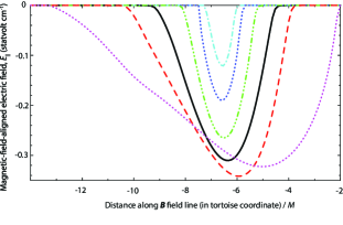
Figure 6.— Spatial distribution of the magnetic-field-aligned electric field, $E_{\parallel}$ (statvolt ${\rm cm}^{-1}$) along the rotation axis, $\theta=0^{\circ}$, for a black hole with $M=10^{9}M_{\odot}$ and $a_{\ast}=0.9$. The cyan dash-dotted, blue dotted, green dash-dot-dot-dotted, red dashed, black solid, and purple dotted curves correspond to $\dot{m}=1.78\times 10^{-4}$, $1.00\times 10^{-4}$, $5.62\times 10^{-5}$, $3.16\times 10^{-5}$, $1.77\times 10^{-5}$, and $5.62\times 10^{-6}$, respectively. The abscissa denotes the tortoise coordinate.

Let us briefly examine how the gap width, $w$, is affected when the ADAF soft photon field changes. In figure 7, we plot the gap inner and outer boundary positions as a function of $\dot{m}$, where the ordinate is converted into the Boyer-Lindquist radial coordinate. It follows that the gap inner boundary (solid curve, $r=r_{1}$), infinitesimally approaches the horizon (dash-dotted horizontal line, $r=r_{\rm H}$), while the outer boundary (dashed curve, $r=r_{2}$) moves outwards, with decreasing $\dot{m}$. At greater accretion rate, $\dot{m}>1.8\times 10^{-4}$, we fail to find stationary solutions. This is because only the photons that are up-scattered in the extreme Klein-Nishina limit can materialize as pairs in the gap, and because the emission of such highest-energy photons suffers substantial fluctuations during the Monte Calro simulation. At smaller accretion rate, $\dot{m}<5.6\times 10^{-6}$, there is no stationary gap solution, because the pair creation becomes too inefficient to create the externally imposed current density, $j$, even when $w\gg M$. Note that $j$ (along each magnetic flux tube) should be constrained by a global requirement (including the dissipative region at large distances), and cannot be solved if we consider only the gap region.

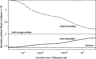
Figure 7.— Spatial extent of the gap along the radial poloidal magnetic field line as a function of the dimensionless accretion rate. The gap is solved for a black hole with $M=10^{9}M_{\odot}$ and $a_{\ast}=0.9$. Thick solid and dashed curves denote the position of the inner and the outer boundaries of the gap, in the unit of the gravitational radius, $GMc^{-2}=M$. These boundary positions (in the ordinate) are transformed from the tortoise coordinate into the Boyer-Lindquist coordinate. The horizontal dash-dotted line shows the horizon radius, whereas the horizontal dotted line does the null surface position on the magnetic axis, $\theta=0$.

5.1.4 Electron distribution function

Because $E_{\parallel}$ is negative, electrons are accelerated outwards while positrons inwards. Thus, the outward $\gamma$-rays, which we observe, are emitted by the electrons. We therefore focus on the distribution function of the electrons created inside the gap.

In figure 8, we plot the electron distribution function, $\gamma n_{-}(r,\gamma)$, along the rotation axis, $\theta=0^{\circ}$, when the accretion rate is $\dot{m}=1.77\times 10^{-5}$. Note that $\gamma n_{-}$ denotes the electron phase-space density per logarithmic Lorentz factor. The abscissa denotes the Lorentz factor, $\gamma$, in logarithmic scale. The ordinate denotes the distance $s$ along the magnetic field line from the null surface, and converted into the Boyer-Lindquist radial coordinate (fig. 2 of H16). Note that $s\approx r-r_{0}$ holds near the rotation axis.

Within the gap, electron-positron pairs are created via photon-photon collisions. Since $E_{\parallel}<0$, electrons are accelerated outward from the lower part of this figure to the upper part. The accelerated electrons lose energy via ICS and distribute between $4\times 10^{7}<\gamma<1.5\times 10^{8}$ in the gap. Although a tiny $|E_{\parallel}|<10^{-4}$, and hence the gap extends upto $r-r_{0}=0.75M$ at $\theta=0^{\circ}$, $|E_{\parallel}|$ falls down to $0.1\mbox{statvolt cm}^{-1}$ at $r-r_{0}=0.57M$ and $10^{-2}\mbox{statvolt cm}^{-1}$ at $r-r_{0}=0.68M$. Thus, the electrons becomes nearly mono-energetic when escaping from the gap, forming a ‘shock’ in the momentum space (due to the concentration of their characteristics) at $r-r_{0}>0.60M$.

In figure 9, we also plot $\gamma n_{-}(r,\gamma)$ at five different positions, $r-r_{0}=-0.249M$, $-0.042M$, $0.164M$, $0.371M$, and $0.716M$. Within the gap, $\gamma$ saturate below $1.5\times 10^{8}$ because of the IC radiation drag. Such low-energy electrons doe not efficiently emit photons via curvature process. Thus, the IC process dominates the curvature one.

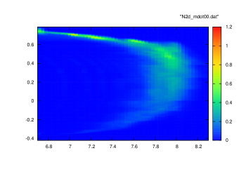
Figure 8.— Distribution function, $\gamma n_{-}$, of the electrons along the magnetic field line on the polar axis, $\theta=0^{\circ}$, for the BH with $M=10^{9}M_{\odot}$ and $a_{\ast}=0.9$, and accretion rate $\dot{m}=1.77\times 10^{-5}$. The abscissa denotes the electron Lorentz factor in $\log_{10}$ scale, while the ordinate does the distance from the null surface, $r-r_{0}$, along the poloidal magnetic field line. The ordinate is converted into the Boyer-Lindquist radial coordinate and plotted in gravitational radius, $M$, unit.

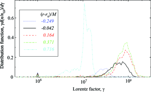
Figure 9.— Distribution function, $\gamma n_{-}$, of the electrons at five positions along the magnetic field line on the polar axis, $\theta=0^{\circ}$, for the BH with $M=10^{9}M_{\odot}$ and $a_{\ast}=0.9$, and accretion rate $\dot{m}=1.77\times 10^{-5}$. The blue dotted, black solid, red dashed, green dash-dotted, and cyan dash-dot-dot-dotted curves denote the $\gamma n_{-}$ at $r-r_{0}=-0.249M$, $-0.042M$, $0.164M$, $0.371M$, and $0.716M$, respectively.

5.1.5 Spectrum of gap emission

The predicted photon spectra are depicted in figure 10 for six $\dot{m}$’s. The thin curves on the left denote the input ADAF spectra, while the thick lines on the right do the output spectra from the gap. We find that the emitted $\gamma$-ray flux increases with decreasing $\dot{m}$, because the potential drop in the gap increases with decreasing $\dot{m}$. The spectral peaks appear between 1 TeV and 30 TeV, because the ICS process dominates the curvature one for such super-massive BHs. The distance is assumed to be 10 Mpc. It is clear that the gap HE flux lies well below the detection limit of the Fermi/LAT (three thin solid curves labeled with “LAT 10 yrs”), . Nevertheless, its VHE flux appears above the CTA detection limits (dashed and dotted curves labeled with “CTA 50 hrs”). . In the flaring state, such a large VHE flux will be detected within one night; thus, it is possible that a nearby low-luminosity, super-massive BH exhibits a detectable gap emission above TeV when the dimensionless accretion rate near the central BH resides in $6\times 10^{-6}<\dot{m}<3\times 10^{-5}$.

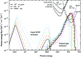
Figure 10.— SED of the gap emission for a super-massive black hole with $M=10^{9}M_{\odot}$ and $a_{\ast}=0.9$, for six discrete dimensionless accretion rates, $\dot{m}$’s, at 10 Mpc. The thin curves denote the input ADAF spectra, while the thick lines do the output gap spectra. The cyan dash-dotted, blue dotted, green dash-dot-dot-dotted, red dashed, black solid, and purple dotted curves correspond to $\dot{m}=1.77\times 10^{-4}$, $1.00\times 10^{-4}$, $5.62\times 10^{-5}$, $3.16\times 10^{-5}$, $1.77\times 10^{-5}$, $5.62\times 10^{-6}$, respectively. The thin solid curves (with horizontal bars) denote the Fermi/LAT detection limits after 10 years observation, while the thin dashed and dotted curves (with horizontal bars) denote the CTA detection limits after a 50 hours observation. Magnetic field strength is assumed to be the equipartition value with the plasma accretion.

5.2. The case of million solar masses

Next, let us consider a smaller BH mass and adopt $M=10^{6}M_{\odot}$. To show the contribution of the curvature process in an extended gap, in this subsection we consider a small accretion rate, $\dot{m}=1.77\times 10^{-5}$, which leads to a reduction of the RIAF photon field, and hence a less effective pair creation and ICS. Because of the increased pair-creation mean-free path, the gap enlarges from $r-r_{0}=-0.549M$ (i.e., almost the horizon) to $r-r_{0}=1.444M$. What is more, because of the decreased ICS optical depth, the curvature process becomes non-negligible compared to the ICS one.

In figure 11, we plot $E_{\parallel}$ (in statvolt ${\rm cm}^{-1}$) as a function of the dimensionless tortoise coordinate, $\eta_{\ast}=r_{\ast}/M$, and the magnetic colatitude, $\theta$ (in degrees), for the dimensionless accretion of $\dot{m}=1.77\times 10^{-5}$. Near the rotation axis, $\theta=0^{\circ}$, much stronger $E_{\parallel}$ arises, in the same way as the $M=10^{9}M_{\odot}$ case (§ 5.1.1).

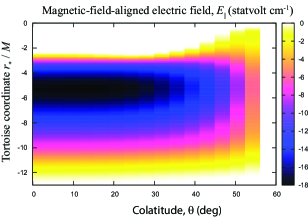
Figure 11.— Similar figure as figure 3 but for $M=10^{6}M_{\odot}$ and $\dot{m}=1.77\times 10^{-5}$.

Let us briefly examine how the gap spatial extent depends on $\dot{m}$, leaving from the fixed value, $1.77\times 10^{-5}$. In figure 12, we plot the gap inner ($r=r_{1}$) and outer ($r=r_{2}$) boundary positions as a function of $\dot{m}$, where the ordinate is converted into the Boyer-Lindquist radial coordinate. In the same way as in the case of $M=10^{9}M_{\odot}$, the gap inner boundary (solid curve), infinitesimally approaches the horizon (dash-dotted horizontal line), while the outer boundary (dashed curve) moves outwards, with decreasing $\dot{m}$. At smaller accretion rate, $\dot{m}<2.3\times 10^{-5}$, there is no stationary gap solution, because the pair creation becomes too inefficient to create the externally imposed current density, $j$, even when $w=r_{2}-r_{1}\gg M$.

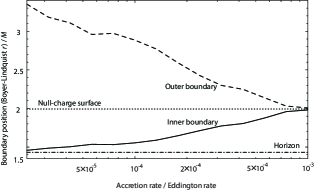
Figure 12.— Similar figure as figure 7 but for $M=10^{6}M_{\odot}$.

Let us return to the case of $\dot{m}=1.77\times 10^{-5}$. In figure 13, we plot the electron distribution function, $\gamma n_{-}(r,\gamma)$. It shows that $\gamma n_{-}$ has a bi-modal distribution on $\gamma$ in the outer half of the gap, $r-r_{0}>0.4M$. The lower-energy peak appears in $10^{7.2}<\gamma<10^{7.4}$. Below $10^{7.2}$, ICS take place in the Thomson regime, because the target RIAF photons are mostly infrared. If the Lorentz factor becomes less than $10^{7.2}$, scattering cross section is almost unchanged, while energy transfer per scattering decreases with decreasing $\gamma$ by $\gamma^{2}$. Thus, $\gamma n_{-}$ peaks slightly above $\gamma\sim 10^{7.2}$. The higher-energy peak appears in $10^{7.85}<\gamma<10^{8.25}$, because the lepton Lorentz factors saturate in this range due to the curvature radiation drag. Unlike stellar-mass BHs (§ 5.1 of H16), however, the curvature component contributes only mildly for SMBHs even when $\dot{m}$ approaches its lower bound ($\dot{m}=1.77\times 10^{-5}$ in the present case) below which a stationary gap solution ceases to exist.

We plot $\gamma n(\gamma,r)$ in figure 14 at five discrete positions, $r-r_{0}$, As electrons are accelerated, their Lorentz factors increase as the blue dotted, black solid, and red dashed lines indicate. When electrons escape from the gap (cyan dash-dot-dot-dotted line), their Lorentz factors concentrate at the terminal values because of the concentration of the characteristics in the momentum space.

In figure 15, we plot the predicted spectra of the gap emissions for six discrete $\dot{m}$’s, assuming a luminosity distance of $1$ Mpc. When the accretion rate is in the narrow range, $2\times 10^{-5}<\dot{m}<3\times 10^{-5}$, we find that the gap emission will be marginally detectable with CTA, particularly if the source is located in the southern sky.

We also plot the emission components for $\dot{m}=1.77\times 10^{-5}$ in figure 16. The black solid line coincides with the purple dotted line in figure 15. The red dash-dotted and red dashed lines represent the IC and curvature components, respectively, while the blue dash-dot-dot-dotted one does the spectrum of the secondary IC and synchrotron photons emitted outside the gap. Because there is a population of electrons saturated at the curvature-limited value for $\dot{m}=1.77\times 10^{-5}$, a weak curvature component appears between 50 MeV and a few GeV.

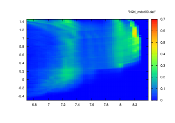
Figure 13.— Similar figure as figure 8 but for $M=10^{6}M_{\odot}$ and $\dot{m}=1.77\times 10^{-5}$. The abscissa denotes the electron Lorentz factor, while the ordinate does the distance from the null surface, $r-r_{0}$, along the poloidal magnetic field line in the Boyer-Lindquist radial coordinate.

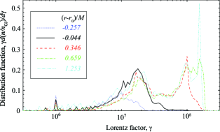
Figure 14.— Similar figure as 9 but for a black hole with $M=10^{6}M_{\odot}$ and $\dot{m}=1.77\times 10^{-5}$. Other parameters are the same: $a_{\ast}=0.9$ and $\theta=0^{\circ}$, The blue dotted, black solid, red dashed, green dash-dotted, and cyan dash-dot-dot-dotted curves denote the $N_{-}$ at $r-r_{0}=-0.257M$, $-0.044M$, $0.346M$, $0.659M$, and $1.253M$, respectively.

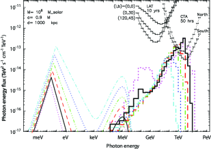
Figure 15.— SED of the gap emission for a super-massive black hole with $M=10^{6}M_{\odot}$ and $a_{\ast}=0.9$, for six discrete dimensionless accretion rates, $\dot{m}$’s, at 1 Mpc. The thin curves denote the input ADAF spectra, while the thick lines do the output gap spectra. The cyan dash-dotted, blue dotted, green dash-dot-dot-dotted, red dashed, black solid, and purple dotted curves correspond to $\dot{m}=3.14\times 10^{-4}$, $1.00\times 10^{-4}$, $5.62\times 10^{-5}$, $4.21\times 10^{-5}$, $3.16\times 10^{-5}$, $1.77\times 10^{-5}$, respectively.

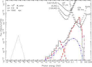
Figure 16.— Similar figure as fig. 15, but only the case of $\dot{m}=1.77\times 10^{-5}$ is depicted. The thick and thin black curves correspond to the same ones in figure 15. The red dashed and dash-dotted lines denote the primary curvature and inverse-Compton (IC) components, respectively. Reprocessed, secondary IC and synchrotron components are are denoted by the blue dash-dot-dot-dotted curve.

6. Discussion

To sum up, we have examined the formation of a stationary lepton accelerator (i.e., a gap) in the magnetospheres of a rotating, super-massive black hole (BH). By solving the set of an inhomogeneous part of the Maxwell equations, lepton Boltzmann equations, and the radiative transfer equation, we demonstrate that the null-charge surface appears in the vicinity of a rapidly rotating BH, and that an electric field arises along the magnetic field line around the null charge surface, in the same manner as in pulsar outer-gap model. In the gap, electrons and positrons are created via two-photon collisions and accelerated in the opposite directions by the magnetic-field aligned electric field into ultra-relativistic energies. Such leptons emit copious $\gamma$-rays mainly via inverse-Compton (IC) processes, leading to a pair-creation cascade in the magnetosphere. The gap longitudinal width is self-regulated so that a single electron eventually cascades into a single pair within the gap, and coincides, on average, with the mean-free path (for an IC photon to materialize via two-photon collision) divided by the number of IC photons emitted by a single electron above the pair-creation threshold energy. As the accretion rate decreases, the increased mean-free path results in an extended gap, and hence an increased luminosity. The gap luminosity, which little depends on the magnetic field configuration near the horizon, maximizes when the gap width becomes greater than the horizon radius. If the BH mass is $M=10^{9}M_{\odot}$, these IC emissions are detectable with CTA, provided that the distance is within a few tens of Mpc and that the dimensionless accretion rate is in the range $6\times 10^{-6}<\dot{m}<3\times 10^{-5}$. If $M=10^{6}M_{\odot}$, they are detectable with CTA, provided that the distance is within a few Mpc and that $2\times 10^{-5}<\dot{m}<3\times 10^{-5}$.

6.1. Improvement form H16

In the present work, there are two major improvements from H16, which formulated the BH gap model and applied it to various BH masses in $10^{1}M_{\odot}<M<10^{9.8}M_{\odot}$.

First, the distribution functions of electrons and positrons are solved as a function of the Lorentz factor, $\gamma$, in the present work, whereas a mono-energetic approximation was adopted in H16. It is found that the Lorentz factors broadly distribute below the saturated value that was estimated in the mono-energetic approximation. This fact causes an important impact on the gap electrodynamics. Since only the highest-energy IC photons contribute in the gap closure (§ 4.2.5), the mono-energetic approximation has overestimated the pair creation in the gap, thereby underestimating the gap width and luminosity (cf. fig. 10 of the present paper and fig.23 of H16). Moreover, the reduced Lorentz factors significantly suppress the curvature process, whose power is proportional to $\gamma^{4}$. Also, the primary IC spectrum is softened to peak between 1–10 TeV in the present work, whereas it peaked between 10–100 TeV in H16. Since CTA increases its sensitivity with decreasing photon energy around 10 TeV, this result encourages us to observe nearby low-luminosity AGNs in VHE.

Second, in the present work, we take into account of an anisotropic and inhomogeneous RIAF specific intensity in computing the IC and pair creation. In particular, it is found that the polar region $\theta\sim 0$ is less efficiently illuminated by the RIAF photon field compared to the middle-latitudes $\theta\sim 45^{\circ}$. It leads to a harder and stronger VHE emission along the rotation axis than that into the middle latitudes. On the contrary, in H16, it was simply assumed that the RIAF photon field was constant for $\theta$. Thus, although the VHE flux decreased with $\theta$ due to the reduced $E_{\parallel}$ near the equatorial boundary, it decreased slower than the present analysis.

6.2. Comparison with pulsar emission models

Let us compare the present BH gap model with the pulsar outer-gap model. In both gap models, the gap appears around the null-charge surface where the GJ charge density vanishes, as the stationary solution of the Maxwell-Boltzmann equations. There are, however, differences as described below.

In pulsar magnetospheres, the neutron star (NS) emits X-ray photons from its surface losing its thermal energy. The luminosity of these soft photons decreases as the NS ages. The decreased soft photon density in the outer magnetosphere results in an extended gap along the magnetic field line. For middle-aged pulsars, $w$ becomes comparable to the radius of the outer light surface, within which the special-relativistic GJ charge density changes substantially due to the convex geometry of the magnetic field lines. In this case, typically $20$ to $30\%$ of the NS spin-down power is dissipated in the gap as HE $\gamma$-rays via the curvature process. Note that the gap efficiency does not approach 100 %, because the exerted $E_{\parallel}$ is less than the vacuum value due to the partial screening by the created and separated pairs, and because the current density is less than the GJ value. The maximum gap power is realized when the current density is between 50% and 70% of the GJ value (i.e., $0.5\leq j\leq 0.7$). Because the photons are emitted along the magnetic field lines that have convex geometry, the HE photons are emitted as a fan-like beam.

In BH magnetospheres, the accreting plasmas emit submillimeter photons from the RIAF. Its luminosity decreases with decreasing accretion rate. The decreases soft photon density near the horizon (typically within a few gravitational radii for rapidly rotating BHs) results in an extended gap width along the magnetic field line. If $\dot{m}<10^{-4}$ for $M\sim 10^{9}M_{\odot}$ or if $\dot{m}<2.3\times 10^{-5}$ for $M\sim 10^{6}M_{\odot}$, the gap longitudinal width becomes comparable to the radius of the inner light surface, within which the GR-GJ charge density changes substantially due to the frame-dragging. In the same way as pulsar outer gaps, typically $20$ to $30\%$ of the BH spin-down power (i.e., the BZ power) is dissipated in the gap as VHE $\gamma$-rays via the IC process from such low-luminosity AGNs. The maximum power is realized if $0.5\leq j\leq 0.7$ (§ 5.1.7 of H16) by the same reason as the pulsar outer gaps. Because photons are preferentially emitted along the magnetic field lines that are nearly radial near the magnetic axis, the VHE photons are emitted as a pencil-like beam, whose geometry is similar to the pulsar polar-cap emission, rather than the outer-gap one.

In pulsar magnetosphere, electrons may be drawn outward as a space-charge-limited flow (SCLF) at the NS surface in the polar-cap region. Thus, in a stationary gap (Harding et al., 1978; Daugherty & Harding, 1982) or in a non-stationary gap (Timokhin & Arons, 2013, 2015), $\gamma$-ray emission could be realized without pair creation within the polar cap, although pairs are indeed created via magnetic pair creation (e.g., at least at the outer boundary where $E_{\parallel}$ is screened). However, in BH magnetospheres, causality prevent any plasma emission across the horizon. Thus, a gap can be sustained only with pair creation, in the same manner as in pulsar outer gaps. In another word, the BH gap electrodynamics is more close to the pulsar outer gap rather than the polar-cap accelerator, although its emission pattern is more close to the latter.

Appendix A Rotating frame of reference

If a frame of reference is rotating with angular frequency $\beta^{\varphi}$, its four velocity $U$ becomes

$$\mbox{\boldmath$e$}_{(\hat{t})}=\mbox{\boldmath$U$}=\frac{dt}{d\tau}\left(\partial_{t}+\beta^{\varphi}\partial_{\varphi}\right),$$ (A1)

where $\mbox{\boldmath$e$}_{(\hat{t})}$ denotes the temporal orthonormal vector basis. The normalization condition, $\mbox{\boldmath$e$}_{\hat{t}}\cdot\mbox{\boldmath$e$}_{\hat{t}}=-1$ gives the redshift factor,

$$\frac{d\tau}{dt}=\sqrt{D},$$ (A2)

where

$$D\equiv-g_{tt}-2g_{t\varphi}\beta^{\varphi}-g_{\varphi\varphi}(\beta^{\varphi})^{2}.$$ (A3)

The clock in this rotating frame delays by the factor $d\tau/dt$ with respect to the distant static observer. Putting

$$\mbox{\boldmath$e$}_{(\hat{\varphi})}=a_{1}\partial_{\varphi}+b_{1}\partial_{t},$$ (A4)

and imposing $\mbox{\boldmath$e$}_{\hat{t}}\cdot\mbox{\boldmath$e$}_{\hat{\varphi}}=0$ and $\mbox{\boldmath$e$}_{\hat{\varphi}}\cdot\mbox{\boldmath$e$}_{\hat{\varphi}}=1$, we obtain

$$a_{1}=-\frac{g_{tt}+g_{t\varphi}\beta^{\varphi}}{\rho_{\rm w}\sqrt{D}}$$ (A5)

and

$$b_{1}=\frac{g_{t\varphi}+g_{\varphi\varphi}\beta^{\varphi}}{\rho_{\rm w}\sqrt{D}}.$$ (A6)

For completeness, we also write the radial and meridional orthonormal bases:

$$\mbox{\boldmath$e$}_{(\hat{r})}=\sqrt{g^{rr}}\partial_{r},$$ (A7)

$$\mbox{\boldmath$e$}_{(\hat{\theta})}=\sqrt{g^{\theta\theta}}\partial_{\theta},$$ (A8)

We can inversely solve equations (A1) –(A8) to obtain the following coordinate bases:

$$\mbox{\boldmath$e$}_{(t)}\equiv\partial_{t}=-\frac{d\tau}{dt}\frac{g_{tt}+g_{t\varphi}\beta^{\varphi}}{D}\mbox{\boldmath$e$}_{(\hat{t})}-\frac{\rho_{\rm w}}{\sqrt{D}}\beta^{\varphi}\mbox{\boldmath$e$}_{(\hat{\varphi})},$$ (A9)

$$\mbox{\boldmath$e$}_{(\varphi)}\equiv\partial_{\varphi}=-\frac{d\tau}{dt}\frac{g_{t\varphi}+g_{\varphi\varphi}\beta^{\varphi}}{D}\mbox{\boldmath$e$}_{(\hat{t})}+\frac{\rho_{\rm w}}{\sqrt{D}}\mbox{\boldmath$e$}_{(\hat{\varphi})},$$ (A10)

$$\mbox{\boldmath$e$}_{(r)}\equiv\partial_{r}=\sqrt{g_{rr}}\mbox{\boldmath$e$}_{(\hat{r})},$$ (A11)

$$\mbox{\boldmath$e$}_{(\theta)}\equiv\partial_{\theta}=\sqrt{g_{\theta\theta}}\mbox{\boldmath$e$}_{(\hat{\theta})}.$$ (A12)

If necessary, we may use the dual one-form bases. From equations (A1), (A4), (A7) and (A8), we obtain

$$\tilde{\omega}^{(\hat{t})}=-\frac{d\tau}{dt}\left(\frac{g_{tt}+g_{t\varphi}\beta^{\varphi}}{D}\tilde{d}t-\frac{g_{t\varphi}+g_{\varphi\varphi}\beta^{\varphi}}{D}\tilde{d}\varphi\right),$$ (A13)

$$\tilde{\omega}^{(\hat{\varphi})}=\frac{\rho_{\rm w}}{\sqrt{D}}\left(\tilde{d}\varphi-\beta^{\varphi}\tilde{d}t\right),$$ (A14)

$$\tilde{\omega}^{(\hat{r})}=\sqrt{g_{rr}}\tilde{d}r,$$ (A15)

$$\tilde{\omega}^{(\hat{\theta})}=\sqrt{g_{\theta\theta}}\tilde{d}\theta,$$ (A16)

References

- Abramowicz et al. (1995) Abramowicz, M., Chen, X., Kato, S., Lasota, J. P. Regev, O. 1995, ApJ, 438, L37
- Beskin et al. (1992) Beskin, V. S., Istomin, Ya. N., & Par’ev, V. I. 1992, Sov. Astron., 36(6), 642
- Blandford & Znajek (1976) Blandford, R. D., & Znajek, R. L. 1976, MNRAS, 179, 433
- Blandford & Begelman (1999) Blandford, R. D., & Begelman, M. C. 1999, MNRAS, 211, L1
- Bogovalov (1999) Bogovalov, S. V. 1999, A&A, 349, 1017
- Boyer & Lindquist (1967) Boyer, R. H. & Lindquist, R. W. 1967 J. Math. Phys., 265, 281
- Broderick & Tchekhovskoy (2015) Broderick, A. E., Tchekhovskoy A. 2015, ApJ, 809, 97
- Carter (1968) Carter, B. 1968, PhRv, 174, 1559
- Cheng et al. (1986a) Cheng, K. S., Ho, C. & Ruderman, M. 1986a, ApJ, 300, 500
- Cheng et al. (1986b) Cheng, K. S., Ho, C. & Ruderman, M. 1986b, ApJ, 300, 522
- Cheng et al. (2000) Cheng, K. S., Ruderman, M. & Zhang, L. 2000, ApJ, 537, 964
- Cheng & Zhang (1996) Cheng, K. S., & Zhang, L. 1996, ApJ, 463, 271
- Chiang & Romani (1992) Chiang, J. & Romani, R. W. 1992, ApJ, 400, 629
- Daugherty & Harding (1982) Daugherty, J. K. & Harding, A. K. 1982, ApJ, 252, 337
- Esin et al. (1997) Esin, A. A., McClintock, J. E., Narayan, R. 1997, ApJ, 489, 865
- Esin et al. (1998) Esin, A. A., Narayan, R., Cui, W., Grove, J. E., Zhang, S. N. 1998, ApJ, 505, 854
- Ferrarese et al. (1996) Ferrarese, L., Ford, H. C., Jaffe, W., 1996, ApJ, 470, 444
- Goldreich & Julian (1969) Goldreich, P., Julian, W. H., 1969, ApJ, 157, 869
- Harding et al. (1978) Harding, A. K., Tademaru, E. & Esposito, L. S. 1978, ApJ, 225, 226
- Harding (1981) Harding, A. K. 1981, ApJ, 245, 267
- Hawley & Krolik (2006) Hawley, J. F., Krolik, J. H. 2006, ApJ, 641, 103
- Hirose et al. (2004) Hirose, S. Krolik, J., de Villiers, J.-P., Hawley, J. F. 2004, ApJ, 606, 1083
- Hirotani & Okamoto (1998) Hirotani, K. & Okamoto, I. 1998, ApJ, 497, 563
- Hirotani & Shibata (1999) Hirotani, K., & Shibata, S. 1999, MNRAS, 308, 54
- Hirotani et al. (2003) Hirotani, K., Harding, A. K., & Shibata, S., 2003, ApJ, 591, 334
- Hirotani (2006a) Hirotani, K. 2006a, ApJ652, 1475
- Hirotani (2006) Hirotani, K. 2006, Mod. Phys. Lett. A (Brief Review), 21, 1319
- Hirotani (2013) Hirotani, K. 2013, ApJ, 766, 98
- Hirotani & Pu (2016) Hirotani, K., Pu, H.-Y. 2016, ApJ, 818, 50 (HP16)
- Hirotani et al. (2016) Hirotani, K., Pu, H.-Y., Lin, L. C.-C., Chang, H.-K., Inoue, M., Kong, A. K. H., Matsushita, S., and Tam, P.-H. T. 2016, ApJ, 818, 50 (H16)
- Hirotani et al. (2016) Hirotani, K., Pu, H.-Y., Lin, L. C.-C., Kong, A. K. H., Matsushita, S., Asada, K., Chang, H.-K., and Tam, P.-H. T. 2016, ApJ, 818, 50 (H16)
- Holloway (1973) Holloway, N. J. 1973, Nature Phys. Sci., 246, 6
- Hujeirat (2004) Hujeirat, A., 2004, A&A, 416, 423
- Ichimaru (1977) Ichimaru, S. 1979, ApJ, 214, 840
- Kerr (1963) Kerr, R. P. 1963, Phys. Rev. Lett., 11, 237
- Koide et al. (2002) Koide, S., Shibata, K., Kudoh, T., Meier, D. L., 2002, Science, 295, 1688
- Larkin et al. (2016) Larkin, A. C., McLaughlin, D. E., 2016, MNRAS, 462, 1864
- Levinson & Rieger (2011) Levinson, A., Rieger, F. 2011, ApJ, 730, 123
- Li et al. (2008) Li, Y.-R., Yuan, Y.-F., Wang, J.-M., Wang, J.-C., Zhang, S. 2008, ApJ, 699, 513
- Lynden-bell (1969) Lynden-bell, D. 1969, Nature, 223, 690
- Mahadevan (1997) Mahadevan, R. 1997, ApJ, 477, 585
- Manmoto (2000) Manmoto, T., 2000, ApJ, 534, 734
- Meier et al. (2001) Meier, D. L., Koide, S., Uchida, U., 2001, Science, 291, 84
- McKinney & Gammie (2004) McKinney, J. C., Gammie C. F., 2004, ApJ, 611, 977
- McKinney (2006) McKinney, J. C., 2006, MNRAS, 368, 1561
- McKinney & Narayan (2007a) McKinney, J. C., Narayan, R., 2007a, MNRAS, 375, 513
- McKinney & Narayan (2007b) McKinney, J. C., Narayan, R., 2007b, MNRAS, 375, 531
- McKinney et al. (2012) McKinney, J. C., Tchekhovskoy, A., Blandford, R. D., 2012, MNRAS, 423, 3083
- Mestel (1971) Mestel L., 1971, Nature, 233, 149
- Misner et al. (1973) Misner, C. W., Thorne, K. S., Wheeler, J. A., 1973, Gravitation (W. H. Freeman. Publication, San Francisco), pp. 875–876. ISBN 0716703343.
- Miyoshi et al. (1995) Miyoshi, M., Moran, J. Herrnstein, J., Greenhill, L., Kakai, N., Diamond, P., Inoue, M. 1995, Nature, 373, 127
- Narayan & Yi (1994) Narayan, R., Yi, I., 1994, ApJ, 428, L13
- Narayan & Yi (1995) Narayan, R., Yi, I., 1995, ApJ, 452, 710
- Neronov & Aharonian (2007) Neronov, A., Aharonian, F. A. 2007, ApJ, 671, 85
- Punsly (2011) Punsly, B. 2011, MNRAS, 418, L138
- Remco (2016) Remco, C. E., Bosch, V. D. 2016, ApJ, 831, 134
- Romani (1996) Romani, R. 1996, ApJ, 470, 469
- Romani, R. & Watters (2010) Romani, R. & Watters, K. P. 2010, ApJ, 714, 810
- Sadowski & Sikora (2010) Sadowski, A. Sikora, M. 2010, å, 517, A18
- Takahashi et al. (1990) Takahashi, M., Nitta, S., Tatematsu, Y., Tomimatsu, A. 1990, ApJ, 363, 206
- Takata et al. (2004) Takata, J., Shibata, S., & Hirotani, K. 2004, MNRAS354, 1120
- Takata et al. (2016) Takata, J., Ng, C. W.. & Cheng, K. S. 2016, MNRAS, 455, 4249
- Timokhin & Arons (2013) Timokhin, A. N., Arons, J., 2013, MNRAS, 429, 20
- Timokhin & Arons (2015) Timokhin, A. N., Harding, A. K., 2015, ApJ, 810, 144
- Tchekhovskoy et al. (2010) Tchekhovskoy, A., Narayan, R., McKinney, J. C. 2010, ApJ, 711, 50
- Pètri & Kirk (2005) Pètri, J. & Kirk, J. G. 2005, ApJ, 627, L37
- Pètri (2013) Pètri, J. 2013, MNRAS, 434, 2636
- Zhang & Cheng (1997) Zhang, J. L. & Cheng, K. S. 1997, ApJ, 487, 370
- Znajek (1977) Znajek, R. L. 1977, MNRAS, 179, 457