Emergence of Calogero family of models in external potentials: Duality, Solitons and Hydrodynamics

Abstract

We present a first-order formulation of the Calogero model in external potentials in terms of a generating function, which simplifies the derivation of its dual form. Solitons naturally appear in this formulation as particles of negative mass. Using this method, we obtain the dual form of Calogero particles in external quartic, trigonometric and hyperbolic potentials, which were known to be integrable but had no known dual formulation. We derive the corresponding soliton solutions, generalizing earlier results for the harmonic Calogero system, and present numerical results that demonstrate the integrable nature of the soliton motion. We also give the collective fluid mechanical formulation of these models and derive the corresponding fluid soliton solutions in terms of meromorphic fields, commenting on issues of stability and integrability.

1 Introduction

The Calogero model and its various generalizations is one of the most studied integrable systems in physics and mathematics [1, 2, 3]. In its most basic form it describes $N$ identical non-relativistic particles in one dimension interacting through two-body inverse-square potentials in the presence of an external harmonic potential. The Hamiltonian of the rational Calogero model in a harmonic trap reads

$${\cal H} = \frac{1}{2}\sum_{j=1}^{N}\big{(}p_{j}^{2}+\omega^{2}x_{j}^{2}\big{)}+\frac{1}{2}\sum_{j,k=1;j\neq k}^{N}\frac{g^{2}}{(x_{j}-x_{k})^{2}},$$ (1)

where $x_{j}$ are the coordinates of the particles, $p_{j}$ are their canonical momenta, and $g$ is the coupling constant. We normalized the mass of the particles to be unity. This model appears in many branches of physics and mathematics and has connections and relevance to fractional statistics, fluid mechanics, spin chains, two-dimensional gravity, strings in low dimensions etc; As a result, it has been studied extensively (see [4, 5, 6, 7] for reviews and a comprehensive list of references).

The above model is classically and quantum mechanically integrable, and can be obtained as a reduction of a matrix system. Several generalizations are also integrable, involving hyperbolic, trigonometric or elliptic mutual potentials, and also general external potentials of quartic type or corresponding trigonometric type [8, 9, 10]. Moreover, integrable generalizations where the particles carry internal degrees of freedom have been proposed [11, 12, 13, 14, 15].

A particular scaling limit (the “freezing trick”) then leads to integrable spin chains with long-range interactions, including the Haldane-Shastry spin model as well as the non-translation invariant harmonic spin chain [16, 17].

A remarkable fact is that the hydrodynamic limit $N\to\infty$ of the system (1) can be found exactly using the methods of collective field theory [18, 19, 20] or using the methods of Ref. [21, 22]. This is quite nontrivial, as writing classical microscopic Hamiltonians in collective fluid mechanical variables usually involves several approximations. By contrast, the Calogero fluid theory reproduces the dynamics of the many-body system to all orders in $1/N$, with any corrections being of nonperturbative nature.

The integrability and other rich properties of the underlying particle systems suggest that the corresponding fluid mechanical equations are also integrable and point to the existence of soliton solutions. This has, indeed, been verified for the free ($\omega=0$) Calogero model [23] as well as the periodic trigonometric (Sutherland) model [23]. A remarkable method of finding multi-soliton solutions was recently proposed [24, 25], relying on a “dual” representation of the model, where the dual particles play the role of “soliton variables”. The existence of such a dual form is far from obvious, and the demonstration that it reduces to the usual Calogero model is quite involved.

The main goal of this paper is to present a first-order formalism based on a generating function (“prepotential”) that makes the self-dual version of the model apparent and greatly simplifies the derivation of its connection to the second-order Calogero equations of motion. Based on this formalism, generalizations are proposed that can, in principle, admit non-identical particles with different masses and particle-dependent interactions. Conditions of stability and reality, subsequently, reduce the system to the dual formulation of the usual Calogero model and its trigonometric and hyperbolic generalizations, but with more general external potentials which, interestingly, turn out to be the integrable quartic or trigonometric potentials found before [8, 9, 10]. In this formulation, soliton solutions can be identified in these more general potentials. Remarkably, solitons behave as regular Calogero particles but with negative mass and complex coordinates. From this starting point, a similar finite dimensional reduction can also be performed in the hydrodynamic model, with the fluid motion parametrized in terms of a finite number of complex parameters representing soliton positions and speeds. Issues of stability and soliton condensation are also discussed

The paper is organized as follows: In Section 2, we introduce our first-order formalism and derive the general form of two-body and external potentials that can be described this way. The solution of the functional equations that appear and derivation of the specific potentials are delegated to the appendices. We examine the stability and reality conditions and establish the appearance of the generalized quartic-type potentials and solitons. In Section 3, we focus on systems with quartic external potentials and derive their dual formulation and soliton solutions. We comment on the mapping of the soliton problem to an electrostatic problem and present numerical solutions that demonstrate the integrable nature of the soliton solutions. In Section 4, we deal with the collective field and fluid mechanical formulation of these models and present the corresponding soliton solutions in terms of meromorphic fields. Finally, in Section 5 we state our conclusions and point to directions of future investigation.

2 General First-Order Formalism of Interacting Systems

In this section, we will formulate the first-order dual equations of motion for a dynamical system of particles in terms of a generating function (prepotential). This formulation greatly simplifies the proof of equivalence of the dual equations with the second-order equations of a Calogero-like system and allows for generalizations involving more general two-body and external potentials.

The starting point is a system of $n$ particles on the line with coordinates $x_{a}$, $a=1,\dots,n$, obeying the first-order equations of motion

$$m_{a}\dot{x}_{a}=\partial_{a}\Phi$$ (2)

with $\Phi$ a function of the $x_{a}$, $\partial_{a}\equiv{\partial\over\partial x_{a}}$, and $m_{a}$ a set of constant “masses”. Taking another time derivative we obtain

$$m_{a}\ddot{x}_{a} = \sum_{b}\partial_{b}\partial_{a}\Phi\,\dot{x}_{b}=\sum_{b}\partial_{a}\partial_{b}\Phi\frac{1}{m_{b}}\partial_{b}\Phi$$ (3)

$$= \partial_{a}\left[\sum_{b}\frac{1}{2m_{b}}\left(\partial_{b}\Phi\right)^{2}\right]$$

This has the form of a standard equation of motion for particles of mass $m_{a}$ inside a potential

$$V=-\sum_{a}\frac{1}{2m_{a}}\left(\partial_{a}\Phi\right)^{2}$$ (4)

such that

$$m_{a}\ddot{x}_{a} = -\frac{\partial V}{\partial x_{a}}$$ (5)

We wish the potential to contain only one-body and two-body terms. Further, the interactions (two-body terms) should depend only on the relative particle distance. So we choose a $\Phi$ of the general form

$$\Phi=\frac{1}{2}\sum_{a\neq b}F_{ab}(x_{ab})+\sum_{a}W_{a}(x_{a})~{},~{}~{}~{}x_{ab}:=x_{a}-x_{b}$$ (6)

By symmetrizing the sum, the $F_{ab}$ can be chosen to satisfy $F_{ab}(x)=F_{ba}(-x)$. This symmetry ensures that the function $F_{ab}$ depends on the difference between $x_{a}$ and $x_{b}$ without caring about the order of particles. This gives us

$$\partial_{a}\Phi=\sum_{b}f_{ab}(x_{ab})+w_{a}(x_{a})$$ (7)

where we defined

$$f_{ab}(x)=-f_{ba}(-x)=F^{\prime}_{ab}(x)~{},~{}~{}~{}w_{a}(x)=W^{\prime}_{a}(x)$$ (8)

We look for conditions for $f_{ab}$ and $w_{a}$ such that the potential contains only one- and two-body terms. We first examine the case of no external potential.

2.1 The case $W_{a}(x)=0$

At the moment, let us ignore $W_{a}(x_{a})$, i.e, consider the case of no external potential. The expression for the potential $V$ then is

$$V=-\sum_{b\neq c,d}\frac{1}{2m_{b}}f_{bc}(x_{bc})f_{bd}(x_{bd})$$ (9)

Let us define from here on the shorthand (and similarly for other functions)

$$f_{ab}\equiv f_{ab}(x_{a}-x_{b})~{},~{}~{}{\rm satisfying}~{}~{}f_{ab}=-f_{ba}$$ (10)

We also define renormalized functions $\tilde{f}_{ab}$,

$$f_{ab}=m_{a}m_{b}\tilde{f}_{ab}$$ (11)

Then the above potential becomes

$$V = -\frac{1}{2}\sum_{b\neq c,d}m_{b}m_{c}m_{d}\tilde{f}_{cb}\tilde{f}_{db}$$ (12)

$$= -\frac{1}{2}\sum_{b\neq c,c=d}m_{b}m_{c}^{2}\tilde{f}_{bc}^{2}-\frac{1}{2}\sum_{b\neq c\neq d}m_{b}m_{c}m_{d}\tilde{f}_{bc}\tilde{f}_{bd}$$

and symmetrizing over the summation indices

$$V = -\frac{1}{4}\sum_{b\neq c}m_{b}m_{c}(m_{b}+m_{c})\tilde{f}_{bc}^{2}$$ (13)

$$-\frac{1}{6}\sum_{b\neq c\neq d}m_{b}m_{c}m_{d}\left[\tilde{f}_{bc}\tilde{f}_{bd}+\tilde{f}_{cb}\tilde{f}_{cd}+\tilde{f}_{db}\tilde{f}_{dc}\right]$$

The term in the last bracket is, in general, a three-body term. We demand that it be, instead, a sum of two-body terms. That is, we impose the condition

$$\tilde{f}_{bc}\tilde{f}_{bd}+\tilde{f}_{cb}\tilde{f}_{cd}+\tilde{f}_{db}\tilde{f}_{dc}=g_{bc}+g_{bd}+g_{cd}$$ (14)

for some functions $g_{ab}(x)$, for all distinct $b$, $c$, $d$.

The above is a functional equation similar to equations encountered in the study of the Lax pair of identical Calogero particles [26] ${\tilde{f}}_{ab}$ and $g_{ab}$ can depend on the particle indices. Its solution can be obtained with methods similar to the ones for the indistinguishable case, and is derived in Appendix A. In general, the solution involves elliptic Weierstrass functions. In this paper we will focus on the simpler case where the functions $g_{ab}$ are constants, that is

$$\tilde{f}_{cb}\tilde{f}_{db}+\tilde{f}_{dc}\tilde{f}_{bc}+\tilde{f}_{bd}\tilde{f}_{cd}=C_{bcd}$$ (15)

where $C_{bcd}$ is a constant independent of $x$. In this case, the three-body term in the potential (13) becomes an irrelevant constant and the potential becomes a sum of two-body terms $V_{ab}$. Up to rescalings of the coordinate $x$, we have the folowing three possibilities for $\tilde{f}_{ab}(x_{ab})$, $F_{ab}(x_{ab})$ and $V_{ab}(x_{ab})$ for various values of $C_{bcd}$, described in Table 1 with $g$ a constant.

Table 1: Solutions to functional equations without external potential

$C_{abc}$	$\tilde{f}_{ab}(x_{ab})$	$F_{ab}(x_{ab})$	$-V_{ab}(x_{ab})$
0	$g/{x_{ab}}$	$g\,m_{a}m_{b}\log\left|x_{ab}\right|$	${g\,m_{a}m_{b}(m_{a}+m_{b})\over 4\,x_{ab}^{2}}$
$-g^{2}$	$g\,{\cot x_{ab}}$	$g\,m_{a}m_{b}\log\left|\sin x_{ab}\right|$	${g^{2}m_{a}m_{b}(m_{a}+m_{b})\over 4\sin^{2}x_{ab}}$
$+g^{2}$	$g\,{\coth x_{ab}}$	$g\,m_{a}m_{b}\log\left|\sinh x_{ab}\right|$	${g^{2}m_{a}m_{b}(m_{a}+m_{b})\over 4\sinh^{2}x_{ab}}$

The above are essentially the rational, periodic and hyperbolic integrable models of Calogero type but with particle-dependent two-body couplings. The integrablity of this generalized version of family of Calogero models (unequal coupling constants and masses) remains unexplored.

2.2 The case $W_{a}(x)\neq 0$ (External Potentials)

We now consider the case where the prepotential includes one-body terms $W_{a}(x_{a})$, leading to a term $w_{a}=W^{\prime}_{a}(x_{a})$ in (7). In analogy with $f_{ab}$ we define

$$w_{a}=m_{a}{\tilde{w}}_{a}$$ (16)

The expression for the potential, using ${\tilde{f}}_{ab}=-{\tilde{f}}_{ba}$ and symmetrizing in the indices, becomes

$$-V = \frac{1}{4}\sum_{b\neq c}m_{b}m_{c}(m_{b}+m_{c})\tilde{f}_{bc}^{2}$$ (17)

$$+ \frac{1}{6}\sum_{b\neq c\neq d}m_{b}m_{c}m_{d}\left[\tilde{f}_{bc}\tilde{f}_{bd}+\tilde{f}_{cb}\tilde{f}_{cd}+\tilde{f}_{db}\tilde{f}_{dc}\right]$$

$$+ \frac{1}{2}\sum_{b\neq c}m_{b}m_{c}({\tilde{w}}_{b}-{\tilde{w}}_{c}){\tilde{f}}_{bc}+\frac{1}{2}\sum_{b}m_{b}{\tilde{w}}_{b}^{2}$$

The terms in the first two lines are the same as for the $W_{a}=0$ case, and the requirement that they reduce to two-body terms gives the same solutions for ${\tilde{f}}_{ab}$ as before. The last line contains two-body and one-body potentials. Demanding that two-body terms depend only on particle distance imposes the condition

$$({\tilde{w}}_{b}-{\tilde{w}}_{c}){\tilde{f}}_{bc}=u_{bc}+v_{b}+v_{c}$$ (18)

for some particle-dependent functions $u_{ab}(x)$ and $v_{a}(x)$. The above is a functional equation for the functions ${\tilde{w}}_{a}$ whose solutions depend on the functions ${\tilde{f}}_{ab}$. Its treatment is given in Appendix B, and we state in Table 2 the solutions in each case, up to rescalings of $x$, with $m_{tot}=\sum_{a}m_{a}$ the total mass, $C_{a},c_{1},c_{2},c_{3}$ constants, and as usual $C_{ab}=C_{a}-C_{b}$.

Table 2: Solutions to functional equations with external potential

$\tilde{f}_{ab}(x_{ab})$	$~{}~{}~{}~{}{\tilde{w}}_{a}(x_{a})$	$~{}~{}~{}u_{ab}(x_{ab})$	$~{}~{}~{}~{}~{}~{}~{}~{}~{}~{}~{}~{}~{}~{}~{}~{}~{}-2V_{a}(x_{a})$
$g/{x_{ab}}$	$C_{a}+c_{1}x_{a}+c_{2}\,x_{a}^{2}+c_{3}\,x_{a}^{3}$	$\frac{gC_{ab}}{x_{ab}}$$-\frac{1}{2}{gc_{3}}x_{ab}^{2}$	$m_{a}{\tilde{w}}_{a}^{2}+g(m_{tot}-m_{a})m_{a}(c_{2}\,x_{a}+{3\over 2}c_{3}\,x_{a}^{2})$
$g\cot x_{ab}$	$C_{a}+c_{1}\cos 2x_{a}+c_{2}\sin 2x_{a}+c_{3}x_{a}$	$gC_{ab}\cot x_{bc}+gc_{3}x_{ab}\cot x_{ab}$	$m_{a}{\tilde{w}}_{a}^{2}+g(m_{tot}-m_{a})m_{a}(c_{2}\cos 2x_{a}-c_{1}\sin 2x_{a})$
$g\coth x_{ab}$	$C_{a}+c_{1}\cosh 2x_{a}+c_{2}\sinh 2x_{a}+c_{3}x_{a}$	$gC_{ab}\coth x_{bc}+gc_{3}x_{ab}\coth x_{ab}$	$m_{a}{\tilde{w}}_{a}^{2}+g(m_{tot}-m_{a})m_{a}(c_{2}\cosh 2x_{a}+c_{1}\sinh 2x_{a})$

In the case that we restrict our solutions to $u_{bc}=0$ (a justification of why this may be relevant is given later), that is, we only allow one-body terms to appear in the right hand side of (18), then $c_{3}$ must vanish and all $C_{a}$ have to be equal. The acceptable forms for ${\tilde{w}}_{a}$ and coresponding one-body potentials are given in Table 3. Interestingly, we recover the restricted form of the integrable potentials found in [8, 9, 10], for which the proof of integrability simplifies considerably. (The most general class of integrable potentials, derived in [9, 10], depends on one additional parameter.)

Table 3: Solutions to functional equations with one-body external potentials

$\tilde{f}_{ab}(x_{ab})$	${\tilde{w}}_{a}(x_{a})$	$-2V_{a}(x_{a})$
$g/{x_{ab}}$	$c_{0}+c_{1}x_{a}+c_{2}x_{a}^{2}$	$m_{a}{\tilde{w}}_{a}^{2}+g(m_{tot}-m_{a})m_{a}c_{2}\,x_{a}$
$g\cot x_{ab}$	$c_{0}+c_{1}\cos 2x_{a}+c_{2}\sin 2x_{a}$	$m_{a}{\tilde{w}}_{a}^{2}+g(m_{tot}-m_{a})m_{a}(c_{2}\cos 2x_{a}-c_{1}\sin 2x_{a})$
$g\coth x_{ab}$	$c_{0}+c_{1}\cosh 2x_{a}+c_{2}\sinh 2x_{a}$	$m_{a}{\tilde{w}}_{a}^{2}+g(m_{tot}-m_{a})m_{a}(c_{2}\cosh 2x_{a}+c_{1}\sinh 2x_{a})$

It would seem peculiar that the eliminated term is the cubic term in the rational case, while it is the linear term in the trigonometric and hyperbolic cases. We can check, however, that the small-$x$ limit of the above trigonometric or hyperbolic potentials, upon proper scaling of the coefficients, reduces to the rational case. In particular, the presence of the linear term in the trigonometric and hyperbolic cases introduces an extra parameter which can be tuned to make the coefficient of $x^{3}$ finite and nonzero in the small-$x$ limit.

2.3 Reality Conditions and Solitons

The potential of the above dynamical system, as given by (4), is negative definite and thus, in principle, unstable. To obtain more interesting stable systems, we extend the variables and parameters to the complex plane. The goal is to find a set of parameters for which the particles, or at least a subset of them, will remain on the real axis and will constitute a stable real dynamical system.

With an appropriate choice of parameters, we can ensure that the potential will turn positive and thus be stable when the $x_{a}$ are on the real axis. This is simply achieved by taking $\Phi\to i\Phi$, that is,

$${\tilde{f}}_{ab}\to i{\tilde{f}}_{ab}~{},~{}~{}{\tilde{w}}_{a}\to i{\tilde{w}}_{a}~{},~{}~{}V\to-V$$ (19)

The first-order equations of motion in terms of $i{\tilde{f}}_{ab}$ and $i{\tilde{w}}_{a}$, however, become

$${\dot{x}}_{a}=i\sum_{b\neq a}m_{b}{\tilde{f}}_{ab}+i{\tilde{w}}_{a}$$ (20)

We observe that even if the initial positions of the particles are real, their velocities will be imaginary and therefore will escape into the complex plane. It is thus impossible to obtain a stable system with all the particle coordinates real.

We demand, therefore, that a subset of the particle coordinates, say $x_{1},\dots x_{N}$, to remain real, while the rest of them, $x_{N+1},\dots x_{n}$, will become complex. For clarity, we call the real coordinates $x_{j}$, $j=1,\dots N$, and the remaining complex ones $z_{\alpha}$, $\alpha=1,\dots M$ with $M=n-N$. For reasons that will become apparent later on, we call the $z_{\alpha}$ “solitons”.

The first basic requirement is that the potential should contain no couplings between $x_{j}$ and $z_{\alpha}$, else such mutual forces would drive the $x_{j}$ into the complex plane. This means, in particular, that the top line in (17) should contain no mixed terms; that is

$$m_{j}m_{\alpha}(m_{j}+m_{\alpha})=0~{}~{}{\rm for~{}all}~{}~{}j,\alpha$$ (21)

The only possibility (other than $m_{j}=0$ or $m_{\alpha}=0$) is

$$m_{j}=-m_{\alpha}=m$$ (22)

That is, all particles have the same (positive) mass, while solitons have the same negative mass. The second line in (17) is a constant in our case, so it is of no concern. The first term in the third line, however, in principle couples particles and solitons, as its mixed terms are

$$m_{j}m_{\alpha}u_{j\alpha}$$ (23)

We thus demand $u_{j\alpha}=0$, which leaves the possibilities found before for vanishing $u_{ab}$. The above conditions will secure that the potential does not couple (real) particles and (complex) solitons and thus their second-order equations of motion decouple. Particles will obey their own Calogero-like equation of motion and solitons will obey their own similar equations.

To make sure that the motion of particles will remain real, we must further ensure that their initial velocities are real. Their expression (for $m_{j}=m$ and $m_{\alpha}=-m$) is

$${\dot{x}}_{j}=im\sum_{k(\neq j)}{\tilde{f}}_{jk}-im\sum_{\alpha}{\tilde{f}}_{j\alpha}+i{\tilde{w}}_{j}$$ (24)

while the corresponding expression for solitons is

$${\dot{z}}_{\alpha}=-im\sum_{k}{\tilde{f}}_{\alpha k}+im\sum_{\beta(\neq\alpha)}{\tilde{f}}_{\alpha\beta}+i{\tilde{w}}_{\alpha}$$ (25)

For real $x_{j}$, the first and last terms in the right hand side of (24) are purely imaginary. Reality of the ${\dot{x}}_{j}$ implies

$$m\sum_{k(\neq j)}{\tilde{f}}_{jk}-m~{}{\rm Re}\left(\sum_{\alpha}{\tilde{f}}_{j\alpha}\right)+{\tilde{w}}_{j}=0$$ (26)

$${\dot{x}}_{j}=m~{}{\rm Im}\left(\sum_{\alpha}{\tilde{f}}_{j\alpha}\right)$$ (27)

The above are, altogether, $2N$ real constraints for $2N+2M$ real variables (the $N$ initial positions $x_{j}$, $N$ initial velocities ${\dot{x}}_{j}$ and the $M$ complex initial values of complex $z_{\alpha}$). Overall, there are $2M$ free parameters in this model, which can be chosen as the initial values of $z_{\alpha}$. (We caution that the parameters $z_{\alpha}$ may not actually uniquely determine the state of the system, as equation (26) may have none or more than one solutions for the $x_{j}$.)

We see that, in general, the real particle system $x_{j}$ follows a motion that is parametrized by the initial values of the $M$ complex soliton parameters $z_{\alpha}$, which can, then, be viewed as phase space variables for the system. The number of solitons $M$ determines the degrees of freedom of the system. In particular, for $M=0$ all velocities are zero and particles are in their equilibrium position determined by (26) for ${\tilde{f}}_{j\alpha}=0$.

For the case $M=1$, $z_{1}(t)$ moves as a solitary particle inside the one-body potential $V(z_{1})$ given in Table 3. Its presence deforms the distribution of $x_{j}$, creating a coalescence of particles near Re$(z_{1}(t))$, that is, a solitary wave. The imaginary part of $z_{1}(t)$ determines the width of the wave, while also determining the velocity of the soliton. For $M>1$ the various $z_{\alpha}$ move as particles in the potential $V(z)$ interacting through Calogero-type potentials, while the real particles $x_{j}$ perform a motion “guided” by the $z_{\alpha}$. The above features justify the identification of $z_{\alpha}$ as soliton parameters, and the corresponding motion of $x_{j}$ as solitonic many-body “waves”.

2.4 Stability

In the previous section we ensured that the dynamical system described by the $x_{j}$ obeys second-order equations of motion in a stable potential. We still need to ensure, however, that the initial value problem as determined by the choice of soliton parameters $z_{\alpha}$ has solutions. As we shall see, this imposes nontrivial constraints.

We start with the simplest case of no solitons. As stated, this corresponds to static $x_{j}$ obeying the condition

$$m\sum_{k(\neq j)}{\tilde{f}}_{jk}+{\tilde{w}}_{j}=0$$ (28)

or, using the definitions of ${\tilde{f}}_{jk}$ and ${\tilde{w}}_{j}$ as well as $m_{j}=m_{k}=m$,

$${\partial\Phi\over\partial x_{j}}=0~{},~{}~{}~{}\Phi=\sum_{j<k}F_{jk}(x_{jk})+\sum_{j}W(x_{j})$$ (29)

These are the equilibrium conditions for particles $x_{j}$ inside the (real) prepotential $\Phi$ defined above. In order for this to have solutions it must be of an appropriate form.

Let us examine the rational case. The prepotential and real potential in this case become

$$\Phi=\sum_{j}\left(c_{0}x_{j}+{c_{1}\over 2}x_{j}^{2}+{c_{2}\over 3}x_{j}^{3}\right)+\sum_{j<k}g\,m\ln|x_{jk}|~{}~{}~{}~{}~{}~{}~{}~{}~{}~{}$$ (30)

$$V=\sum_{j}\left[{m\over 2}\left(c_{0}+c_{1}x_{j}+{c_{2}}x_{j}^{2}\right)^{2}+g(N-1)m^{2}c_{2}x_{j}\right]+\sum_{j<k}{g\,m^{2}\over x_{ab}^{2}}$$ (31)

The prepotential consists of a cubic one-body potential and a logarithmic two-body interaction. We can always choose the sign of $g$ that makes the interaction term repulsive, $g<0$ (in the opposite case we can flip the sign of $g$ as well as $c_{0},c_{1},c_{2}$ which leads to the same potential $V$). So this becomes a standard problem of finding the equilibrium position of particles in a potential with repulsive logarithmic interactions.

Generically, this problem may not have solutions since the cubic potential is unbounded from below. This happens, in particular, for the simplest nontrivial purely cubic case ($c_{0}=c_{1}=0$). To guarantee the existence of solutions the prepotential must have a “well” such that it can trap particles. The existence of such a well requires the condition

$$c_{1}^{2}>4c_{0}c_{2}$$ (32)

This condition is necessary but not sufficient. The well must also be deep enought to hold $N$ particles repelling each other with a logarithmic interaction of strength $gm$. We have no explicit expressions for this restriction in terms of the constants of the problem. We stress that the above restrictions are necessary so that the equilibrum problem can be addressed in the first-order formalism. The real potential $V$, being a quartic expression in the coordinate, always has an equilibrium solution.

For a nonzero number of solitons the situation becomes more complicated, as now the set of equations (26, 27) must admit solutions. In general this will imply restrictions to both the form of the potential and the range of “phase space” parameters $z_{\alpha}$. We point out, however, that the interaction between particles and solitons is attractive, so in general the presence of solitons improves the situation. In fact, it may be that the unstable prepotentials for which the zero-soliton case has no static solutions become stable in the presence of a large number of solitons, akin to a “broken” symmetry phase with a soliton condensate. We postpone the investigation of this issue for a future publication.

2.5 A Note on Integrability

Solitons are a hallmark of integrability and, indeed, Calogero-like systems are one of the most celebrated classes of integrable models. The systems derived here, however, differ from standard Calogero models in the fact that (i) the particles are not identical, with distinct masses and corresponding two-body interactions, and (ii) in the presence of a more general one-body potential.

In the above analysis, the issue of integrability remains unaddressed. There are, nevertheless, some intriguing indications that these systems are integrable. First, the reality conditions necessary to have stable potentials naturally restrict the system to identical particles ($m_{j}=m$) which is integrable. Further, the extended one-body potentials that we obtained (quartic in the rational case, harmonic with two nontrivial modes in the trigonometric and hyperbolic cases) are exactly the potentials that are know to be integrable [9, 10].

In fact, the obtained potentials belong to a somewhat restricted class. Specifically, a generic quartic potential has 4 nontrivial parameters (ignoring the constant term). Our potential, however, has only 3 parameters ($c_{0},c_{1},c_{2}$), being essentially a complete square. Although arbitrary quartic potentials are integrable, for the above restricted potentials of “Bogomolny” type the proof of integrability simplifies considerably [9, 10, 8].

Finally, an inspection of the known integrals of motion for the standard quadratic Calogero model ($c_{3}=0$) reveals that they are all zero. (This is not a contradiction, since particles and solitons contribute with opposite signs.) Although this is not yet a proof of integrability, since the value of higher integrals could fluctuate between particles and solitons, it is a tantalizing clue that a general proof of integrability may well be possible within the first-order formalism. This and other issues are saved for future investigation.

3 Dual representation and solitons of the rational model in external quartic potentials

In this section we focus on the particular concrete example of rational Calogero models in external quartic potentials. Using the general formalism of the previous section, we demonstrate the existence of a dual version involving soliton variables $z_{\alpha}$ and derive analytical and numerical solutions.

3.1 First order equations for the rational Calogero case

The general formalism discussed above greatly helps in writing down the first order equations for the rational Calogero case. If we take the first row of Table 2 and impose that particles (indexed by $j$) have mass $m_{j}=1$ and solitons (indexed by $\alpha$) have mass $m_{\alpha}=-1$, then (24) and (25) give

$$\dot{x}_{j}-iw(x_{j}) = -ig\sum_{k=1(k\neq j)}^{N}\frac{1}{x_{j}-x_{k}}+ig\sum_{\alpha=1}^{M}\frac{1}{x_{j}-z_{\alpha}},$$ (33)

$$\dot{z}_{\alpha}-iw(z_{\alpha}) = ig\sum_{\alpha=1(\alpha\neq\beta)}^{M}\frac{1}{z_{\alpha}-z_{\beta}}-ig\sum_{j=1}^{N}\frac{1}{z_{\alpha}-x_{j}},$$ (34)

for $x_{j}(t)$ with $j=1,2,\ldots,N$ and $z_{\alpha}(t)$ with $\alpha=1,2,\ldots,M$. Here, the function $w$ is given in Table 3 as

$$w(x)=c_{0}+c_{1}x+c_{2}x^{2}$$ (35)

Since both $w_{a}$ and $V_{a}$ are independent of the particle index $a$ (see Table 3), we dropped the subscripts.

Equations (33,34) are first order in time and, for complex coordinates, the dynamics is fully defined by the initial values of $x_{j}$, $z_{\alpha}$, i.e., by $N+M$ complex numbers ($2N+2M$ real variables). If the particle coordinates $x_{j}$ are real (with real velocities), as discussed in section 2.3, the dynamics is fully determined by the $M$ complex initial values of $z_{\alpha}$. Applying Eq. (4) of the general formalism, the corresponding second order equations are given by

$$\ddot{x}_{j} = -\frac{g^{2}}{2}\frac{\partial}{\partial x_{i}}\sum_{i\neq j}^{N}\frac{1}{\left(x_{i}-x_{j}\right)^{2}}-V^{\prime}(x_{j}),\qquad j=1,\dots,N$$ (36)

$$\ddot{z}_{\alpha} = -\frac{g^{2}}{2}\frac{\partial}{\partial z_{\alpha}}\sum_{\alpha=1(\alpha\neq\beta)}^{M}\frac{1}{\left(z_{\alpha}-z_{\beta}\right)^{2}}-V^{\prime}(z_{\alpha}),\qquad\alpha=1,\dots,M$$ (37)

We refer to the system (33,34) as the dual Calogero system in external potential $V$. We emphasize that the general formalism greatly simplifies the transition from first order to second order equations. Lack of such a general formalism would have involved a laborious algebra to arrive at the second order equations (36,37). We also point out that the derivation of (36,37) from (33,34) holds for arbitrary $N$ and $M$, although we are mostly interested in the case $M<N$.

3.2 Multi-Soliton solutions

From the first order equations derived above for the rational Calogero model, we get (separating real and imaginary parts of (33)),

$$w(x_{j}) = g\sum_{k=1(k\neq j)}^{N}\frac{1}{x_{j}-x_{k}}-\frac{g}{2}\sum_{\alpha=1}^{M}\left(\frac{1}{x_{j}-z_{\alpha}}+\frac{1}{x_{j}-\bar{z}_{\alpha}}\right),$$ (38)

$${\dot{x}}_{j}=p_{j} = i\frac{g}{2}\,\sum_{\alpha=1}^{M}\left(\frac{1}{x_{j}-z_{\alpha}}-\frac{1}{x_{j}-\bar{z}_{\alpha}}\right).$$ (39)

As we noted in section 2.3, if we specify the $M$ complex positions $z_{\alpha}$ at any time we can find both the $N$ real positions $x_{j}$ and the corresponding real momenta $p_{j}$. If we are given the initial values of $x_{j}$ and $p_{j}$, their evolution is fully determined by (36). However, these initial values are not, in general, independent, as they are related by (38,39) through the values of the $M$ complex parameters ($2M$ real parameters) $z_{\alpha}$ . (Only when $M\geq N$ we can choose them independently.) The initial values of ${\dot{z}}_{\alpha}$ are always restricted, as they need to satisfy (34) and the $x_{j}$ are fully fixed by the $z_{\alpha}$.

3.3 Solution for zero solitons

In this section we discuss the case of zero solitons. This gives rise to a spacially inhomogeneous static background configuration where all particles are at rest. (We also note that this is the same as the limit where all $z_{\alpha}$ go to infinity.) Taking $M=0$ we have $p_{j}=0$ for all $j$ and the particle coordinates settle in the equilibrium positions

$$w(x_{j})=c_{0}+c_{1}x_{j}+c_{2}x_{j}^{2}=g\sum_{k=1(k\neq j)}^{N}\frac{1}{x_{j}-x_{k}}.$$ (40)

If we just had a harmonic trap as in [24, 25], in which case $w^{harm}(x)=\omega x$, then it is known that the solution of this system of algebraic equations is given by the roots of the $N$-th Hermite polynomial (Stiltjes formula [27, 30]). We are unaware of a generalization of the Stiltjes formula when $w(x)$ has a quadratic form as above.

3.4 The single-soliton solution

The single soliton case is essentially equivalent to one complex $z$ coordinate moving freely in a quartic polynomial potential. For $M=1$ equations (38,39) become

$$c_{0} + c_{1}x_{j}+c_{2}x_{j}^{2}=g\sum_{k=1(k\neq j)}^{N}\frac{1}{x_{j}-x_{k}}-\frac{g}{2}\left(\frac{1}{x_{j}-z}+\frac{1}{x_{j}-\bar{z}}\right),$$ (41)

$$p_{j} = i\frac{g}{2}\left(\frac{1}{x_{j}-z}-\frac{1}{x_{j}-\bar{z}}\right).$$ (42)

Equation (41) is a further generalization of the Stieltjes problem (40) (see Refs. [27, 28, 29]). To our understanding, exact solutions of (41) are not known (not even in the case of harmonic potential), and the solution may not be unique. Equation (41) is essentially the equilibrium position of $N$ particles repelling each other but held in an external potential and also attracted to an additional particle of opposite “charge”, as will be further elaborated in section 3.6.

The soliton is a single particle moving in an external quartic polynomial potential. That is, equation (37) in the case $M=1$ takes the simple form

$$\ddot{z}=-V^{\prime}(z)=-k_{3}z^{3}-k_{2}z^{2}-k_{1}z-k_{0}$$ (43)

where $k_{0},\dots,k_{3}$ are related to the parameters of the model (see Table 3 and eq. (31)). This is a single anharmonic complex oscillator. Typically, analytical solutions for the above equation are not available for quartic polynomials $V(z)$, but solving a single particle problem is numerically easy. Knowing the value of $z(t)$, we then use (41) and (42) to find the $x_{j}$ and $p_{j}$. The upper left panel of Fig. 1 demonstrates the particle evolution profile for the case of a single solition. We see that the worldline of particles clearly shows a robust soliton. The motion of the corresponding variable $z(t)$ is given in the lower left panel of the same Fig. 1.

3.5 The two-soliton solution

The case when the system has two solitons is nontrivial even with respect to the $z_{1},z_{2}$ variables. In this case, we have two complex soliton coordinates in a quartic potential interecting with Calogero forces. Putingt $M=2$ in (38,39) we obtain

$$w(x_{j}) = g\sum_{k=1(k\neq j)}^{N}\frac{1}{x_{j}-x_{k}}-\frac{g}{2}\Big{(}\frac{1}{x_{j}-z_{1}}+\frac{1}{x_{j}-\bar{z}_{1}}$$

$$+ \frac{1}{x_{j}-z_{2}}+\frac{1}{x_{j}-\bar{z}_{2}}\Big{)},$$

$$p_{j} = i\frac{g}{2}\left(\frac{1}{x_{j}-z_{1}}-\frac{1}{x_{j}-\bar{z}_{1}}+\frac{1}{x_{j}-z_{2}}-\frac{1}{x_{j}-\bar{z}_{2}}\right)$$ (45)

while solitons obey the coupled second-order equations

$$\ddot{z}_{1} = -\frac{g^{2}}{2}\frac{\partial}{\partial z_{1}}\sum_{i\neq j}^{M}\frac{1}{\left(z_{1}-z_{2}\right)^{2}}-V^{\prime}(z_{1})$$ (46)

$$\ddot{z}_{2} = -\frac{g^{2}}{2}\frac{\partial}{\partial z_{2}}\sum_{i\neq j}^{M}\frac{1}{\left(z_{2}-z_{1}\right)^{2}}-V^{\prime}(z_{2})$$ (47)

Initial conditions for ${\dot{z}}_{1,2}$ can be set by specifying $z_{1,2}$ and using (3.5) to find $x_{j}$ and then (34) to find ${\dot{z}}_{1,2}$. Then the evolution of $z_{1,2}$ can be found by solving the above Calogero equations.

The upper right panel of Fig. 1 shows the particle evolution profile in the case of two solitions. We see that the worldline of particles clearly shows two robust solitons, one moving left and another moving right. The motion of the corresponding complex soliton variables is given in the lower right panel of the same Fig. 1.

3.6 Mapping solitons to an electrostatic problem and the numerical protocol

Let us take a close look at equation (38). It is essentially the derivative of the real part of the prepotential $\Phi$:

$$U=Real(\Phi) = \sum_{j=1}^{N}W(x_{j})-\sum_{j<k}\ln|x_{j}-x_{k}|$$ (48)

$$+ \frac{1}{2}\sum_{j=1}^{N}\sum_{n=1}^{M}\Big{[}\ln|x_{j}-z_{\alpha}|+\ln|x_{j}-\bar{z}_{\alpha}|\Big{]}.$$

where we remind the reader that the function $W(x)$ is related to $w(x)$ as

$$W(x)=\int_{0}^{x}w(x^{\prime})dx^{\prime}$$ (49)

Eq. (38) is then the extremum condition ${\partial U\over\partial x_{j}}=0$ for the above function.

The function $U$ can be thought of as the “electrostatic energy” of $N$ particles with unit charges interacting through a logarithmic potential (2d Coulomb potential), restricted to move along a straight line (the real axis) and in the presence of $2M$ external charges $-1/2$ placed at $z_{\alpha},\bar{z}_{\alpha}$ and of an external potential $W(x)$. The solution of (38) is not necessarily a minimum of (48), but may correspond to any fixed point (maximum, minimum or saddle point) of (48), and there may be several such points.

The above observation forms the basis for a numerical procedure for solving Eq. (38), at least for solutions corresponding to a local minimum. The basic idea is to let the particles slide towards the minimum of the above potential by introducing a “viscous” force that allows them to move towards their equilibrium positions. That is, we introduce the following $N$ coupled ODEs

$$\dot{x}_{j}=-\gamma\frac{\partial{U}}{\partial x_{j}}$$ (50)

It is clear that the above drives the system to the minimum of the potential $U$. In fact, the above equation implies

$$\frac{dU}{dt}=-\frac{\gamma}{2}\sum_{j=1}^{N}\left(\frac{\partial{U}}{\partial x_{j}}\right)^{2}$$ (51)

so the potential decreases until it reaches a fixed point. Local maxima can also be dealt this way by flipping the sign of $U$ and ttuning them into minima. Saddle points, on the other hand, will be missed.

The above first-order equation can be integrated numerically. Once we find the solutions for $x_{j}$, we then use Eq. (42) to find the initial momenta. These form the special initial conditions for the particles that correspond to a set of solitons, and we can evolve them according to Eq. 36 without further reference to the soliton variables.Therefore, we have mapped the problem of finding soliton configurations to an electrostatic problem of a function $U$.

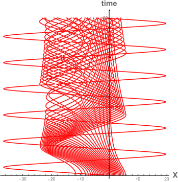
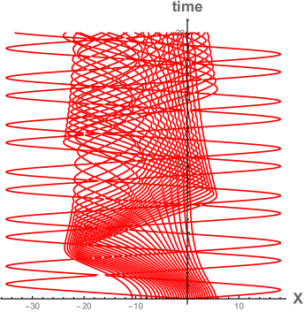
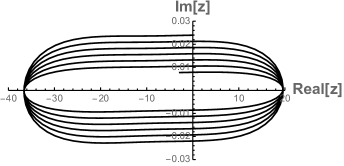
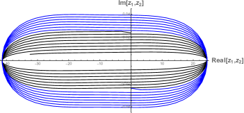
Figure 1: (Upper Panel Left) One soliton solution for rational Calogero model in external quartic polynomial potential. Here we take N=31 particles and the special initial condition is dictated by a single $z=0.0239i$. We notice, in the worldine picture, a remarkable evidence of a robust soliton We use the prepotential $w(x)=x+0.06x^{2}$ which makes the potential $V(x)=0.87x+0.5x^{2}+0.06x^{3}+0.0018x^{4}$ using first row of Table 3. (Lower Panel Left) We show the motion of one dual variable “z” corresponding to one soliton solution. The initial condition is $z(t=0)=0.0239i$ and $\dot{z}(t=0)=-43.0768-0.00103378i$ (which is fixed by Eq. 34) and the equation it satifies is $\ddot{z}=-V^{\prime}(z)$ where $V(z)=0.93z+0.5z^{2}+0.06z^{3}+0.0018z^{4}$ again using first row of Table 3. (Upper Panel Right) Two soliton solution where initial conditions are dictated by two values of dual variable, $z_{1}=+0.0239i$ and $z_{2}=-0.0239i$. We use the prepotential $w(x)=x+0.06x^{2}$ which makes the potential $V(x)=0.84x+0.5x^{2}+0.06x^{3}+0.0018x^{4}$ using first row of Table 3. We see clear evidence of two solitons in the system. (Lower Panel Right) Motion of two coupled dual variables $z_{1}$ (black) and $z_{2}$ (blue) is shown here. They satisfy the equation $\ddot{z}_{1}=g^{2}\frac{1}{(z_{1}-z_{2})^{3}}-V^{\prime}(z_{1})$ where $V(z)=0.9z_{1}+0.5z_{1}^{2}+0.06z_{1}^{3}+0.0018z_{1}^{4}$ (similarly for the other dual variable $z_{2}$). The initial conditions are $z_{1}(t=0)=+0.0239i$, $z_{2}(t=0)=-0.0239i$, $\dot{z}_{1}(t=0)=-64.297-0.00129161i$, $\dot{z}_{2}(t=0)=64.297-0.00129161i$.

4 Hydrodynamic Limit and Meromorphic Fields

4.1 General formalism

In this section we consider the generalized Calogero models with external potentials and take the hydrodynamic limit to derive soliton solutions for the corresponding fluid mechanical density and velocity of the particles. We do this by introducing specific meromorphic functions with poles on the position of particles and solitons and taking their many-particle limit. The approach is related to the one of [21, 22], but we will give an independent simplified exposition, directly following from our first-order formulation.

We consider a system with $N$ (real) particle coordinates $x_{j}$ and $M$ (complex) solitons $z_{\alpha}$. We will take the prepotential to be of the form that ensures a stable potential and absence of 3-body forces, as found in section 2, leading to the first-order equations (20)

$${\dot{x}}_{a}=i\sum_{b}m_{b}{\tilde{f}}_{ab}+i{\tilde{w}}_{a}$$ (52)

and corresponding second-order equations

$${\ddot{x}}_{a}=-{1\over m_{a}}\partial_{a}V=-\partial_{a}\left[\sum_{b(\neq a)}\frac{1}{2}m_{b}(m_{a}+m_{b}){\tilde{f}}_{ab}^{2}+(m_{tot}-m_{a})v_{a}+\frac{1}{2}{\tilde{w}}_{a}^{2}\right]$$ (53)

with $v_{a}=v(x_{a})$ and ${\tilde{w}}_{a}={\tilde{w}}(x_{a})$ as found in section 2.2. Coordinates $x_{a}$ run over particles (for $a=j$) and solitons ($a=\alpha$), and we take the masses of particles to be $m_{j}=1$ and the masses of solitons $m_{\alpha}=-1$, so $m_{tot}=N-M$.

To this system we add one more “spectator” particle $a=0$ with coordinate $x_{0}=x$ and mass $m_{0}$. The full system of $N+M+1$ particles and total mass $N-M+m_{0}$ retains its Calogero-like form. Using Eq. 52 for this spectator particle, the velocity $u$ of the spectator particle is, in particular,

$$u={\dot{x}} = i\sum_{a\neq 0}m_{a}{\tilde{f}}(x-x_{a})+i{\tilde{w}}(x)$$ (54)

$$= i\sum_{j=1}^{N}{\tilde{f}}(x-x_{j})-i\sum_{\alpha=1}^{M}{\tilde{f}}(x-z_{\alpha})+i{\tilde{w}}(x)$$

and its corresponding acceleration (using Eq. 53) is

$${du\over dt}={\ddot{x}} = -\partial_{x}\left[\sum_{j=1}^{N}{1+m_{0}\over 2}{\tilde{f}}(x-x_{j})^{2}+\sum_{\alpha=1}^{M}{1-m_{0}\over 2}{\tilde{f}}(x-z_{\alpha})^{2}\right.$$ (55)

$$~{}~{}~{}~{}~{}~{}~{}~{}~{}+\left.(N-M)\,v(x)+\frac{1}{2}{\tilde{w}}(x)^{2}\right]$$

The additional particle $x$ creates an additional term $m_{0}{\tilde{f}}(x_{a}-x)$ in the equation for ${\dot{x}}_{a}$ of the remaining particles, and a corresponding term in the potential. We wish this particle to be a spectator, that is, not to modify the motion of the remaining particles (while itself being influenced by them). So we take the limit $m_{0}\to 0$, which leaves the $N$ particles and solitons the same as in the original $N+M$-particle Calogero-like system. Equation (54) for $u={\dot{x}}$ remains unchanged, while the equation for ${\ddot{x}}$ becomes

$${du\over dt} = -\partial_{x}\Bigg{[}\sum_{j}\frac{1}{2}{\tilde{f}}(x-x_{j})^{2}$$ (56)

$$+ \sum_{\alpha}\frac{1}{2}{\tilde{f}}(x-z_{\alpha})^{2}+(N-M)v(x)+\frac{1}{2}{\tilde{w}}(x)^{2}\Bigg{]}$$

The role of the spectator particle is that it monitors and essentially determines both the position and the velocity of the remaining particles. To this end, we consider $u$ as defined in (54) as a function of the spectator particle position $x$ and promote $x$ to an independent variable, defining a field $u(x)$. The time derivative of $u(x)$, written as ${\partial u\over\partial t}$, is thus the time variation of $u$ arising from its dependence on $x_{j}(t)$ and $z_{\alpha}(t)$, but not on $x$. In other words, we define,

$${\partial u\over\partial t}\equiv\sum_{j}{\partial u\over\partial x_{j}}{\dot{x}}_{j}+\sum_{\alpha}{\partial u\over\partial z_{\alpha}}{\dot{z}}_{\alpha}$$ (57)

The total time derivative entering (56) is, therefore,

$${du\over dt} = {\partial u\over\partial x}{\dot{x}}+\sum_{j}{\partial u\over\partial x_{j}}{\dot{x}}_{j}+\sum_{\alpha}{\partial u\over\partial z_{\alpha}}{\dot{z}}_{\alpha}$$ (58)

$$= u\partial_{x}u+{\partial u\over\partial t}=\partial_{x}\left(\frac{1}{2}u^{2}\right)+{\partial u\over\partial t}$$

where we used ${\dot{x}}=u$ and the definition Eq. 57.

The above relation and (56) allow us to find the equation of motion of the field $u(x,t)$. To do this, we need to express the terms involving $x_{j}$ and $z_{\alpha}$ in (56) in terms of $u$. This can be achieved by noting that all prepotentials ${\tilde{f}}(x)$ found in section 2.2 (rational, trigonometric or hyperbolic) satisfy the relation

$${\tilde{f}}(x)^{2}=g\,\partial_{x}{\tilde{f}}(x)+C~{},~{}~{}~{}f(x)=-{g\over x},~{}-g\cot x,~{}-g\coth x$$ (59)

where $C$ is a constant (zero, $+g^{2}$ and $-g^{2}$ for rational, hyperbolic and trigonometric prepotential respectively). Therefore the terms involving sums of ${\tilde{f}}^{2}$ in (56) can be expressed as derivatives of terms in $u(x)$. We note, however, that particle and soliton terms come with opposite sign in $u(x)$, while they have the same sign in (56). This necessitates splitting $u(x)$ into two parts:

$$u^{+}(x) = -i\sum_{\alpha}{\tilde{f}}(x-z_{\alpha})+i\lambda{\tilde{w}}(x)$$ (60)

$$u^{-}(x) = i\sum_{j}{\tilde{f}}(x-x_{j})+i(1-\lambda){\tilde{w}}(x)$$ (61)

$$u(x) = u^{+}(x)+u^{-}(x)$$

where $\lambda$ is an arbitrary parameter that splits the term ${\tilde{w}}(x)$ between the two functions. Using (56,58, 59) and (60,61) we arrive at the equation of motion for $u$

$${\partial u\over\partial t} + \partial_{x}\Bigg{[}\frac{1}{2}u^{2}+{ig\over 2}\partial_{x}(u^{+}-u^{-})$$ (62)

$$+ \frac{1}{2}{\tilde{w}}^{2}+(N-M)v+(\lambda-{\textstyle\frac{1}{2}})\,g\,\partial_{x}{\tilde{w}}\Bigg{]}=0$$

The terms independent of $u$ above are the one-body potential $V(x)$ entering the equation of motion of particles $x_{j}$, with the difference that $v(x)$ is multiplied by $N-M$ (rather than $N-M-m_{j}=N-M-1$ and the extra term involving $\partial_{x}{\tilde{w}}(x)$. In fact, for all cases of $\tilde{f}$ (rational, trigonometric and hyperbolic), $\partial_{x}{\tilde{w}}(x)$ is proportional to $v(x)$:

$$g\,\partial_{x}{\tilde{w}}(x)=-2v(x)$$ (63)

The equation for $u(x,t)$ therefore takes the form:

$${\partial u\over\partial t}+\partial_{x}\left[\frac{1}{2}u^{2}+{ig\over 2}\partial_{x}(u^{+}-u^{-})+V+(\lambda-1)g\,\partial_{x}{\tilde{w}}\right]=0$$ (64)

If we want the equation of motion of $u$ to involve the same one-body potential $V(x)$ as that of particles, we must choose $\lambda=1$, assigning the full prepotential ${\tilde{w}}(x)$ to $u^{+}$. This is in fact the opposite convention than the one in [22], where $u^{-}$ contains the term ${\tilde{w}}(x)$. We stress that any choice of $\lambda$ is allowed, leading to different definitions of $u^{+}$, $u^{-}$ and an extra term in the evolution equation for $u$. We also note that $\lambda$ does not appear in the equation of $u$ (64) in the quadratic (harmonic) rational Calogero case studied in Ref. [22], since $w(x)$ is linear and $v(x)$ is a constant that drops from the equation.

4.2 The rational case and derivation of the hydrodynamic limit

The above construction holds for all three types of Calogero potentials. We first examine the rational case. We pick $\lambda=1$ as the most natural choice and define

$$u^{+}(x) = ig\sum_{\alpha=1}^{M}\frac{1}{x-z_{\alpha}}+i{\tilde{w}}(x)$$ (65)

$$u^{-}(x) = -ig\sum_{j=1}^{N}\frac{1}{x-x_{j}}$$ (66)

A priori, it looks like we have a single equation of motion (64) for two fields $u^{+}$ and $u^{-}$. As we stressed before, however, the particle system is actually fully determined by the values of $z_{\alpha}$, so in principle $u^{+}$ is enough to fully fix the system. $u^{+}$ is a meromorphic function of $x$ with $M$ simple poles at $z_{\alpha}$, so it fixes the number of solitons. Using the equations of motion (33) we see that $u^{+}$ satisfies

$$u^{+}(x_{j})={\dot{x}}_{j}+ig\sum_{k=1(k\neq j)}^{N}\frac{1}{x_{j}-x_{k}}.$$ (67)

Therefore, if we also know that there are $N$ particles, the function $u^{+}(x)$ fully determines the system, as:

$$Im~{}u^{+}(x_{j})=g\sum_{k=1(k\neq j)}^{N}\frac{1}{x_{j}-x_{k}}$$ (68)

$$Re~{}u^{+}(x_{j})={\dot{x}}_{j}=v_{j}$$ (69)

The $N$ equations (68) in principle determine the $N$ real variables $x_{j}$, and subsequently (69) determines ${\dot{x}}_{j}$. The known values of $x_{j}$, then, determine the function $u^{-}(x)$ through equation (66).

The definition of $u^{+}(x)$, (see Eq. 65) however, does not involve $N$, and the same function $u^{+}(x)$ can describe systems of an arbitrary number of particles (see Eq. 68, 69). The real part of $u^{+}(x)$ for real $x$, in particular, defines a continuous velocity field $v(x)$ that is the actual particle velocity on the position of particles. Similarly, its imaginary part defines a field that can be related to the position of particles, for any number of them. It is, therefore, a good tool to deal with the hydrodynamic limit $N\to\infty$ where the interparticle distance goes to zero and the system is described by a continuous density $\rho(x)$ and velocity $v(x)$.

From the above discussion it follows that, in the $N\to\infty$ limit, the real part of $u^{+}(x)$ straightforwardly goes over to the fluid velocity field $v(x)$. To express the imaginary part in terms of the fluid particle density requires a bit more work. In particular, we need to express the sum in (68) in terms of the particle density $\rho(x)$, including all perturbative corrections in $1/N$. This is nontrivial because of the singularity as $x_{k}$ approaches $x_{j}$ and has to be evaluated carefully. This has been done in [31]. Here we will follow a slightly different approach that will allow us to separate the perturbative and non-perturbative parts.

For a large number of particles we define the continuous position function $x(s)$ such that $x(j)=x_{j}$. For finite $N$ any smooth interpolation between the $x_{j}$ will do, while in the $N\to\infty$ limit this function becomes unique. It is related to the continuous density $\rho(x)$ by

$$x^{\prime}(s)={1\over\rho(x(s))}$$ (70)

The sum of interest is

$$\sum_{k(\neq j)=1}^{N}{1\over x_{j}-x_{k}}=\sum_{k(\neq j)=1}^{N}{1\over x(j)-x(k)}$$ (71)

which needs to be expressed in terms of $x(s)$ or $\rho(x)$.

Our starting point is the identity

$$\sum_{n=-\infty}^{\infty}f(n)=\sum_{n=-\infty}^{\infty}{\tilde{f}}(2\pi n)$$ (72)

where $f(s)$ is any function of $s$ and ${\tilde{f}}(q)$ is its Fourier transform, defined as

$${\tilde{f}}(q)=\int_{-\infty}^{\infty}ds~{}e^{-iqs}f(s)$$ (73)

For a function smooth at the scale of $\Delta s\sim 1$, the Fourier transform ${\tilde{f}}(2\pi n)$ for $n\neq 0$ will be negligibly small. In fact, terms with $n\neq 0$ are nonperturbative in $1/N$ (instanton corrections), as we will explain in the sequel. So, up to nonperturbative corrections

$$\sum_{n=-\infty}^{\infty}f(n)={\tilde{f}}(0)=\int_{-\infty}^{\infty}ds~{}f(s)$$ (74)

To apply this formula to the sum (71) we view the summand as a function of $k$ and define it to be zero for $k$ outside its range, extending the summation to all integers. Still, a straightforward application of (74) is hindered by the fact that the summed function $1/[x(j)-x(s)]$ is not smooth, due to the singular behavior near $s=j$, and thus higher Fourier modes contribute substantially. We can proceed in two different ways. The first is to evaluate the higher Fourier modes and sum their contribution. The second is to regularize the integrand in a way that renders it smooth, as was done in [31]. Both methods lead to the same result. Following the second method, we define the function

$$f(s)={1\over x(j)-x(s)}+{1\over x^{\prime}(j)(s-j)+\epsilon(s-j)^{3}}~{},~{}~{}f(j)={x^{\prime\prime}(j)\over 2x^{\prime}(j)^{2}}$$ (75)

for $\epsilon>0$. The above function is continuous everywhere and smooth at the scale of $\Delta s\sim 1$, since the singularity at $s=j$ is subtracted by the second (regulator) term. Summing it over integer values of $s$ we have

$$\sum_{k=-\infty}^{\infty}f(k) = f(j)+\sum_{k(\neq j)=-\infty}^{\infty}f(k)$$ (76)

$$= {x^{\prime\prime}(j)\over 2x^{\prime}(j)^{2}}+\sum_{k(\neq j)=-\infty}^{\infty}{1\over x(j)-x(k)}$$

since the sum of the regulator term is absolutely convergent (due to $\epsilon$) and vanishes due to antisymmetry in $k-j$. Applying (74) we have the result

$$\sum_{k(\neq j)=-\infty}^{\infty}{1\over x(j)-x(k)} = -{x^{\prime\prime}(j)\over 2x^{\prime}(j)^{2}}+\int_{-\infty}^{\infty}f(s)ds$$ (77)

$$= -{x^{\prime\prime}(j)\over 2x^{\prime}(j)^{2}}+P.V.\int_{-\infty}^{\infty}{ds\over x(j)-x(s)}$$

where $P.V.$ stands for principal value. Finally, changing integration variable from $s$ to $y=x(s)$ and using $x^{\prime}=1/\rho$ and thus $x^{\prime\prime}=-\partial_{x}\rho/\rho^{3}$ we obtain

$$\sum_{k(\neq j)=-\infty}^{\infty}{1\over x-x(k)} = {\partial_{x}\rho(x)\over 2\rho(x)}+P.V.\int_{-\infty}^{\infty}{\rho(y)dy\over x-y}$$ (78)

$$= \frac{1}{2}\partial_{x}\ln{\rho(x)}-\pi\rho^{H}(x)$$

where we put $x(j)=x$, and $\rho^{H}(x)$ is the Hilbert transform of $\rho(x)$.

The above result is perturbatively exact in $1/N$. Indeed, the higher Fourier modes of $f(s)$ expressed in terms of $y=x(s)$ are

$${\tilde{f}}(q)=\int_{-\infty}^{\infty}dy\,\rho(y)~{}e^{-iq\int_{-\infty}^{y}dw\,\rho(w)}\,f(s(y))$$ (79)

For a continuous particle distribution, $x(j+1)-x(j)\sim 1/N$, $\rho(x)\sim N$, and thus the oscillating exponent in the above expression for $q\neq 0$ is of order $N$. The integral is thus of order $e^{-N}$, which is nonperturbative in $1/N$. So the $q=0$ term captures the full perturbative contribution. Overall, from (68,69) we obtain for $u^{+}(x)$

$$u^{+}(x)=v(x)-i\pi g\rho^{H}(x)+ig\,\partial_{x}\ln{\sqrt{\rho(x)}}$$ (80)

Nonperturbative contributions are in general negligible in the fluid limit ($N\to\infty$). The one instance in which they become relevant is when the distribution of particles breaks into two or more disjoint components. In this case the distance $x(K)-x(K+1)$ between the last particle $K$ in one component and the first particle $K+1$ in the next is large, and thus the function $f(s)$ is not smooth at $s=K$. The appearance of multiple fluid components signals the onset of nonperturbative effects and needs to be described in terms of multiple functions $\rho_{a}(x)$, one for each component, with compact disjoint supports. In our paper, we do not encounter this scenario and hence, emergence of relavant perturbative corrections is not a concern.

The continuous version of $u^{-}(x)$ can similarly be found. Its definition (66) involves the parameter $x$ and a sum over the full set of particles. By taking the variable $x$ to be complex and off the real axis the issue of singularities is avoided and the summand becomes a smooth function of $x(s)$. So, up to nonperturbative contributions,

$$u^{-}(x)=-ig\sum_{j}\frac{1}{x-x(j)}=-ig\int ds\,\frac{1}{x-x(s)}=-ig\int dy\,{\rho(y)\over x-y}$$ (81)

So $u^{-}(x)$ is the Cauchy transform of $\rho(x)$. As $x$ approaches the real axis the above expression has a discontinuity. We obtain

$$u^{-}(x\pm i0)=\mp\pi g\rho+i\pi g\rho^{H}$$ (82)

with the discontinuity

$$u^{-}(x+i0)-u^{-}(x-i0)=-2\pi g\rho(x).$$ (83)

Expressions (80) and (82) determine $u^{\pm}(x)$ in terms of fluid quantities. Note that with our choice of $\lambda=1$ in the definition (60,61) of $u^{\pm}(x)$ their expression involves only the fluid density $\rho(x)$ and velocity $v(x)$ and not the prepotential ${\tilde{w}}(x)$. Substituting these expressions into the equation (64) for $u(x)$ we obtain in principle 4 real equations (2 for the real part and 2 for the imaginary part at $x\pm i0$) for the two real fields $\rho(x)$ and $v(x)$. These equations are compatible and reduce to the fluid equations

$$\partial_{t}\rho + \partial_{x}(\rho v)=0~{}~{}~{}~{}~{}~{}~{}~{}~{}~{}~{}~{}~{}~{}~{}~{}~{}~{}~{}~{}~{}~{}~{}~{}~{}~{}~{}~{}~{}~{}~{}~{}~{}~{}~{}$$ (84)

$$\partial_{t}v + \partial_{x}\Bigg{[}\frac{1}{2}v^{2}+{\pi^{2}g^{2}\over 2}\rho^{2}+\pi g^{2}\partial_{x}\rho^{H}$$

$$- {g^{2}\over 8}\left(\partial_{x}\ln{\rho}\right)^{2}-{g^{2}\over 4}\partial_{x}^{2}\ln{\rho}+V\Bigg{]}=0$$

The above equations can be seen to arise from the Hamiltonian

$$H=\int dx\left[\frac{1}{2}\rho v^{2}+{\pi^{2}g^{2}\over 6}\rho^{3}+{\pi g^{2}\over 2}\rho\,\partial_{x}\rho^{H}+{g^{2}}{(\partial_{x}\rho)^{2}\over 8\rho}+\rho V\right]$$ (86)

using the standard fluid mechanical Poisson structure

$$\{\rho(x),v(y)\}=\delta^{\prime}(x-y)$$ (87)

4.3 One soliton solution of Calogero model with quartic potentials in terms of meromorphic fields

The one-soliton solution is given by

$$u^{+}(x)=\frac{ig}{x-z_{1}(t)}+i{\tilde{w}}(x),$$ (88)

The single soliton solution for $u^{+}(x)$ is a meromorphic function with a single pole. $z_{1}(t)$ above satisfies (34) for $M=1$ which is simply

$$\dot{z}_{1}-i{\tilde{w}}(z_{1})=-ig\sum_{j=1}^{N}\frac{1}{z_{1}-x_{j}}$$ (89)

and the second-order equation

$${\ddot{z}}_{1}=-V^{\prime}(z_{1})$$ (90)

From the expression of $u^{+}(x)$ in terms of hydrodynamic quantities

$$v-ig(\pi\rho^{H}-\partial_{x}\log\sqrt{\rho})=\frac{ig}{x-z_{1}}+i{\tilde{w}}(x)$$ (91)

we can, in principle, find the density and velocity fields from the position $z_{1}$. Writing $z_{1}(t)=a(t)+ib(t)$ and taking the real and imaginary parts of (91) we obtain

$$v = -g\,\frac{b}{(x-a)^{2}+b^{2}}$$ (92)

$$\pi\rho^{H} - \partial_{x}\log\sqrt{\rho}=-\frac{x-a}{(x-a)^{2}+b^{2}}-{1\over g}{\tilde{w}}(x)$$ (93)

So $a(t)$ parametrizes the position of the soliton while $b(t)$ parametrizes its width. The second equation above needs to be solved for $\rho(x)$. This is nontrivial, although the solution can be found analytically in the limit of thin solitons. In this limit, the width $b\rightarrow 0$, and the soliton solution (upto $O(1/N)$ corrections), can be written as

$$\rho_{sol}(x,t)=\rho_{0}+\delta(x-a(t))$$ (94)

where the background density $\rho_{0}$ satisfies, $\pi\rho_{0}^{H}-\partial_{x}\log\sqrt{\rho_{0}}+{1\over g}{\tilde{w}}(x)=0$

The soliton parameter $z_{1}(t)$ is moving in the complex plane along a non-trivial curve guided by its quartic polynomial as in (90). Therefore, (92,93) give a one-dimensional reduction of an infinite dimensional rational Calogero system with quartic potential in the hydrodynamic limit. The procedure to go to the hydrodynamic limit can similarly be extended for the two-soliton and multi-soliton case.

5 Conclusions and Outlook

To summarize, in this paper we introduced a first order formalism based on a prepotential and derived its general form that gives rise to two-body and external potentials. Imposing the requirements of stability and reality conditions, we demonstrated the natural emergence of the Calogero family of models in generalized quartic and trigonometric external potentials. Our general formalism provides a relatively straightforward route to finding soliton solutions, a task otherwise considered to be an enormous challenge. Using the more common version of the Calogero family of models, namely, the rational Calogero model (in quartic polynomial external potentials), we demonstrate the existence of soliton solutions. We derived the particle time evolution for the case when the system has one and two solitons and we showed that our method can be easily extended to $M$ solitons. We showed that finding soliton solutions can be achieved via a mapping to an electrostatic problem. Using a fluid formalism involving meromorphic fields, we have also identified soliton solutions in the hydrodynamic limit.

One of the the main lesson from the work presented in this paper is that there may exist further extensions of the Calogero family of models beyond the known systems, and that they may admit dual formulations that identify their collective degrees of freedom and provide solutions to their fluid mechanical versions. Clearly, there are many open issues and directions of possible future research.

The most immediate questions are the ones on stability and integrability. It is puzzling that the dual formulation of the quartic potential model is stable only within a subset of its parameters, which actually exclude the purely quartic case. Although we conjecture that models outside the stability regime correspond to a soliton condensate, an explicit demostration of this fact, and derivation of the soliton solutions, would be desirable.

Similarly, our approach does not deal with integrability. Again, it is remarkable that the systems that can be dealt with this formalism do fall eventually within a subclass of the generalized Calogero models that were known to be integrable. A direct derivation of integrability seems to be possible within this formalism and, if there, has yet to be uncovered.

Extension of our results to other members of the Calogero family is also an open issue. We restricted our derivation to the rational, trigonometric and elliptic models and their external potential generalizations, mainly for reasons of mathematical clarity and simplicity. An extension to the elliptic (Weierstrass) model is well within the reach of the formalism. In this context, the identification of elliptic models with external potentials would be a very interesting advance. Similar remarks hold for models of particles with internal degrees of freedom. Clearly an extension of the formalism is needed to incorporate internal particle coordinates, and this is a topic of further research.

Finally, there exist several intriguing similarities of the present formalism with quantum mechanical features of the Calogero model, although our treatment is purely classical. The generating function clearly alludes to a quantum mechanical wavefunction, at least in the equilibrium semiclassical limit. Similarly, the stable and unstable domains of quartic dual systems are in direct analogy with the broken and unbroken phases of supersymmetric quantum mechanical systems, the “unstable” broken phase leading to a soliton condensate. Aspects of our formalism also bear similarities with techniques from matrix models and the exchange operator formulation. These and related issues are left for future investigation.

6 Acknowledgments

M. K. gratefully acknowledges the Ramanujan Fellowship SB/S2/RJN-114/2016 from the Science and Engineering Research Board (SERB), Department of Science and Technology, Government of India. A.P.’s research is supported by NSF grant 1213380 and by a PSC-CUNY grant.

7 Appendix A: Solutions to the functional equations without external potentials

In this Appendix we provide the solutions to the functional equations for ${\tilde{f}}_{ab}$, thereby yielding Table 1. We start with the equation (15) for a fixed triplet of indices $b,c,d$:

$$\tilde{f}_{bc}\tilde{f}_{bd}-\tilde{f}_{bc}\tilde{f}_{cd}+\tilde{f}_{bd}\tilde{f}_{cd}=C_{bcd}$$ (95)

where we used the antisymmetry of ${\tilde{f}}_{ab}=-{\tilde{f}}_{ba}$ to put the indices $b,c,d$ in order.

Let us define, $x\equiv x_{b}-x_{c}$, $y\equiv x_{c}-x_{d}$ such that $x+y=x_{b}-x_{d}$. For convenience, we also rename the doublets of indices $bc\equiv 1$, $cd\equiv 2$, $bd\equiv 3$ and call $C_{bcd}$ simply $C$. The above equation, then, reads

$$\tilde{f}_{1}(x)\tilde{f}_{3}(x+y)-\tilde{f}_{1}(x)\tilde{f}_{2}(y)+\tilde{f}_{3}(x+y)\tilde{f}_{2}(y)=C$$ (96)

In terms of the reciprocal functions $g_{j}(x)=\frac{1}{{\tilde{f}}_{j}(x)}$ the above becomes

$$g_{1}(x)+g_{2}(y)-g_{3}(x+y)=Cg_{1}(x)\,g_{2}(y)\,g_{3}(x+y)$$ (97)

and solving for $g_{3}$ we obtain

$$g_{3}(x+y)=\frac{g_{1}(x)+g_{2}(y)}{1+Cg_{1}(x)g_{2}(y)}$$ (98)

Taking derivatives with respect to $x$ and $y$ and equating the results (since $\partial_{x}g_{3}(x+y)=\partial_{y}g_{3}(x+y)$) we obtain

$$\frac{g_{1}^{\prime}(x)}{1-Cg_{1}^{2}(x)}=\frac{g_{2}^{\prime}(y)}{1-Cg_{2}^{2}(y)}=k={\rm constant}$$ (99)

The above differential equations determine $g_{1}$ and $g_{2}$ and, through (98), they also determine $g_{3}$. Their solution depends on the sign of the constant $C$. Specifically

$$C=0: g_{j}(x)=kx+b_{j}$$

$$C=-g^{2}<0: g_{j}(x)=\frac{1}{g}\sin(kgx+g\,b_{j})$$

$$C=g^{2}>0: g_{j}(x)=\frac{1}{g}\sinh(kgx+g\,b_{j})$$

$$j=1,2,3, {\rm with}~{}~{}b_{1}+b_{2}=b_{3}$$ (100)

Repeating the above analysis for a triplet involving one new particle, say, $b,c,e$, leads to the same equations (99), with the same constants $C$ and $k$ (fixed by the form of $g_{bc}=g_{1}$ found above). Inductively, we conclude that the constants $C=C_{abc}$ and $k$ are common for the full set of particles, while the constants $b_{ab}$ satisfy $b_{ab}+b_{bc}=b_{ac}$ for all $a,b,c$. These constants can actually be absorbed by a shift in the position of particle coordinates:

$$x_{a}\to x_{a}-\frac{b_{1a}}{k}~{},~{}~{}b_{11}\equiv 0$$ (101)

where we chose arbitrarily particle $1$ as a reference, so we can take all $b_{a}=0$. Finally, the constant $k$ can be set to $1/g$ through the rescaling of coordinates $x_{a}\to(kg)^{-1}x_{a}$. Overall, we recover the ${\tilde{f}}_{ab}=1/g_{ab}$ as given in Table 1.

8 Appendix B: Solutions to functional equations for external potentials

In this Appendix we derive the solutions to the functional equation (18), written explicitly as

$$\big{[}{\tilde{w}}_{b}(x_{b})-{\tilde{w}}_{c}(x_{c})\big{]}\,{\tilde{f}}_{bc}(x_{bc})=u_{bc}(x_{bc})+v_{b}(x_{b})+v_{c}(x_{c})$$ (102)

We define $x_{b}=t+s$ and $x_{c}=t-s$, which implies $x_{bc}=2s$. Using also the inverse functions $g_{bc}=1/{\tilde{f}}_{bc}$ defined in the previous Appendix, the above equation becomes

$${\tilde{w}}_{b}(t+s)-{\tilde{w}}_{c}(t-s) = g_{bc}(2s)\bigg{[}u_{bc}(2s)+v_{b}(t+s)+v_{c}(t-s)\bigg{]}$$ (103)

$$= h_{bc}(s)+g_{bc}(2s)\bigg{[}v_{b}(t+s)+v_{c}(t-s)\bigg{]}$$

where we defined $h_{bc}(s)=g_{bc}(2s)u_{bc}(2s)$. The solution of this equation depends on the form of $g_{bc}$ and we treat it in a case-by-case basis for the solutions derived in the previous Appendix.

8.1 The rational case $g_{bc}={1\over{\tilde{f}}_{bc}}=\frac{1}{g}x_{bc}$

In the rational case (103) becomes

$${\tilde{w}}_{b}(t+s)-{\tilde{w}}_{c}(t-s) = {2s\over g}\bigg{[}u_{bc}(2s)+v_{b}(t+s)+v_{c}(t-s)\bigg{]}$$ (104)

$$= h_{bc}(s)+{2s\over g}\bigg{[}v_{b}(t+s)+v_{c}(t-s)\bigg{]}$$

with $h_{bc}(s)=2s\,u_{bc}(2s)/g$. The left hand side is regular around $s=0$ and has a well-defined Taylor expansion in $s$, therefore so must be $h_{bc}(s)$. Expanding in powers of $s$ we obtain

$$s^{0}: {\tilde{w}}_{b}(t)-{\tilde{w}}_{c}(t)=h_{bc}(0)$$ (105)

$$s^{1}: {\tilde{w}}_{b}^{\prime}(t)+{\tilde{w}}_{c}^{\prime}(t)=h_{bc}^{\prime}(0)+{2\over g}\big{[}v_{b}(t)+v_{c}(t)\big{]}$$ (106)

$$s^{2}: {\tilde{w}}_{b}^{\prime\prime}(t)-{\tilde{w}}_{c}^{\prime\prime}(t)=h_{bc}^{\prime\prime}(0)+{4\over g}\big{[}v_{b}^{\prime}(t)-v_{c}^{\prime}(t)\big{]}$$ (107)

$$s^{3}: {\tilde{w}}_{b}^{\prime\prime\prime}(t)+{\tilde{w}}_{c}^{\prime\prime\prime}(t)=h_{bc}^{\prime\prime\prime}(0)+{6\over g}\big{[}v_{b}^{\prime\prime}(t)+v_{c}^{\prime\prime}(t)\big{]}$$ (108)

Eq. (105) states that ${\tilde{w}}_{b}(t)$ and ${\tilde{w}}_{c}(t)$ differ by a constant. Differentiating (106) twice with respect to $t$ and combining with (108) we obtain

$${\tilde{w}}_{b}^{\prime\prime\prime}(t)=-{1\over 4}h_{bc}^{\prime\prime\prime}(0)={\rm constant}$$ (109)

which means that ${\tilde{w}}_{b}$ and ${\tilde{w}}_{c}$ must be of the form

$${\tilde{w}}_{b,c}(t)=C_{b,c}+c_{1}t+c_{2}t^{2}+c_{3}t^{3}$$ (110)

The constants $C_{b}$ and $C_{c}$ can differ, but $c_{1},c_{2},c_{3}$ are the same for any two particles $b$ and $c$, therefore they are common to the system. Substituting this form for ${\tilde{w}}_{b,c}(t)$ in (105-108), or directly in (104), we obtain $v_{b}(x)$, $v_{c}(x)$, $h_{bc}(x)$ and $u_{bc}(x)$. In doing this, we note that the constant terms of $v_{b}$, $v_{c}$ and $u_{bc}$ can be combined together; similarly, $v_{b}^{\prime}(0)-v_{c}^{\prime}(0)$ and $u_{bc}^{\prime}(0)$, contributing a term proportional to $x_{b}-x_{c}=x_{bc}$, can also be combined. We use this to choose $v_{b}(0)=v_{c}(0)=v_{b}^{\prime}(0)-v_{c}^{\prime}(0)=0$. We eventually obtain

$${\tilde{w}}_{b,c}(x) = C_{b,c}+c_{1}x+c_{2}x^{2}+c_{3}x^{3}$$ (111)

$$v_{b,c}(x) = gc_{2}x+{3g\over 2}c_{3}x^{2}$$ (112)

$$u_{bc}(x) = g{C_{b}-C_{c}\over x_{bc}}+gc_{1}-{g\over 2}c_{3}x^{2}$$ (113)

The above recover the potentials presented in Table 2. Note that the constant $gc_{1}$ in $u_{bc}$ is dynamically irrelevant and can be omitted. Note also that the contribution of $v_{a}(x_{a})$ in the full potential involves a sum $\sum_{a\neq b}m_{a}m_{b}v_{a}=\sum_{a}(m_{tot}-m_{a})m_{a}v_{a}$, which explains the coefficient of the corresponding terms in $V_{a}(x_{a})$.

8.2 The trignometric case $g_{bc}={1\over{\tilde{f}}_{bc}}={1\over g}\tan x_{bc}$

In the trignometric or hyperbolic case we proceed in a similar way, Taylor expanding (103) in $s$. The equations are the same as in the previous section for orders $s^{0}$, $s^{1}$ and $s^{2}$, since $\tan x$ is the same as $x$ up to quadratic order. At order $s^{3}$, however, we get instead of (108)

$${\tilde{w}}_{b}^{\prime\prime\prime}(t)+{\tilde{w}}_{c}^{\prime\prime\prime}(t)=h_{ab}^{\prime\prime\prime}(0)+{6\over g}\big{[}v_{b}^{\prime\prime}(t)+v_{c}^{\prime\prime}(t)\big{]}+{16\over g}\big{[}v_{b}(t)+v_{c}(t)\big{]}$$ (114)

Combining this with the other equations yields

$${\tilde{w}}_{b}^{\prime\prime\prime}(t)+4{\tilde{w}}_{b}^{\prime}(t) = -{1\over 4}h_{bc}^{\prime\prime\prime}(0)+2h_{bc}^{\prime}(0)\equiv{\rm C}$$

$${\rm or}~{}~{}{\tilde{w}}_{b}^{\prime\prime}(t)+4{\tilde{w}}_{b}(t) = {\rm C}t+{\rm C}^{\prime}$$ (115)

This is like a driven harmonic oscillator of frequency $2$, with general solution of the form

$$w_{b,c}(t)=C_{b,c}+c_{1}\cos 2t+c_{2}\sin 2t+c_{3}t$$ (116)

Putting this form in the remaining equations, or in the original functional equation, we finally find

$${\tilde{w}}_{b,c}(x) = C_{b,c}+c_{1}\cos 2x+c_{2}\sin 2x+c_{3}x$$ (117)

$$v_{b,c}(x) = g\,c_{2}\cos 2x-g\,c_{1}\sin 2x$$ (118)

$$u_{bc}(x) = g(C_{b}-C_{c})\cot x+g\,c_{3}\,x\cot x$$ (119)

The hyperbolic case is treated in exactly the same way, or can be obtained by simple analytic continuation $x\to ix$, $g\to ig$, $c_{2}\to-ic_{2}$. Altogether, we recover the potentials presented in Table 2.

References

References

- [1] F. Calogero, J. Math. Phys. 10, 2191 (1969). Solution of a Three-Body Problem in One Dimension. ibid. 10, 2197 (1969); Ground State of a One-Dimensional -Body System. ibid. 12, 419 (1971). Solution of One-Dimensional -Body Problems with Quadratic and/or Inversely Quadratic Pair Potentials.
- [2] B. Sutherland, Phys. Rev. A 4, 2019 (1971); Exact Results for a Quantum Many-Body Problem in One Dimension. ibid., 5, 1372 (1972). Exact Results for Quantum Many-Body Problem in One Dimension. II. Phys. Rev. Lett. 34, 1083 (1975). Exact Ground-State Wave Function for a One-Dimensional Plasma.
- [3] J. Moser, Adv. Math. 16, 197 (1975). Three integrable Hamiltonian systems connected with isospectral deformations
- [4] M. A. Olshanetsky and A. M. Perelomov, Phys. Rep. 71, pp. 313-400, (1981), Classical integrable finite-dimensional systems related to Lie algebras; Phys. Rep. 94, Issue 6, pp. 313-404 (1983), Quantum Integrable Systems Related to Lie Algebras.
- [5] For a review and original references see A. M. Perelomov, Integrable Systems of Classical Mechanics and Lie Algebras., Birkhäuser Basel (1989).
- [6] For a review and original references see B. Sutherland, Beautiful Models: 70 Years Of Exactly Solved Quantum Many-Body Problems., World Scientific, (2004).
- [7] Alexios P Polychronakos, Journal of Physics A: Mathematical and General, Volume 39, Number 41, The physics and mathematics of Calogero particles
- [8] V.I. Inozemtsev, Physica Scripta 29 (1984) 518-520., New completely integrable multiparticle dynamical systems
- [9] Alexios Polychronakos, Phys.Lett. B276 (1992) 341-346 A New integrable system with a quartic potential
- [10] Alexios P. Polychronakos, Phys.Lett. B277 (1992) 102-108 New integrable systems from unitary matrix models
- [11] N. Kawakami, Phys. Rev. B46, 1005 (1992). Asymptotic Bethe-ansatz solution of multicomponent quantum systems with long-range interaction
- [12] N. Kawakami, Phys. Rev. B46, 3191 (1992). SU(N) generalization of the Gutzwiller-Jastrow wave function and its critical properties in one dimension
- [13] Z.N.C. Ha and F.D.M. Haldane, Phys. Rev. B46, 9359 (1992), Models with inverse-square exchange
- [14] J.A. Minahan and A. P. Polychronakos, Phys. Lett. B302, 265 (1993) [arXiv:hep-th/9206046]. Integrable Systems for Particles with Internal Degrees of Freedom
- [15] K. Hikami and M. Wadati, Phys. Lett. A173, 263 (1993). Integrable spin-12 particle systems with long-range interactions
- [16] Alexios P. Polychronakos, Phys.Rev.Lett. 70 (1993) 2329-2331, Lattice Integrable Systems of Haldane-Shastry Type
- [17] Alexios P. Polychronakos, Nucl.Phys. B419 (1994) 553-566, Exact Spectrum of SU(n) Spin Chain with Inverse-Square Exchange
- [18] A. Jevicki and B. Sakita, Nucl. Phys. B165, 511 (1980). The Quantum Collective Field Method and its Application to the Planar Limit.
- [19] B. Sakita, Quantum Theory of Many-variable Systems and Fields., World Scientific, 1985.
- [20] A. Jevicki, Nucl. Phys. B376, 75-98 (1992). Nonperturbative Collective Field Theory.
- [21] A. G. Abanov and P. B. Wiegmann, Phys. Rev. Lett 95, 076402 (2005). Quantum Hydrodynamics, the Quantum Benjamin-Ono equation, and the Calogero Model.
- [22] A. G. Abanov, E. Bettelheim and P. Wiegmann, J. Phys. A: Math. Theor. 42, 135201 (2009). Integrable hydrodynamics of Calogero-Sutherland model: bidirectional Benjamin-Ono equation.
- [23] A. P. Polychronakos, Phys. Rev. Lett. 74, 5153 (1995). Waves and Solitons in the Continuum Limit of the Calogero-Sutherland Model.
- [24] A. G Abanov, A. Gromov and M. Kulkarni, Journal of Physics A: Mathematical and Theoretical, Volume 44, Number 29, 17 June 2011. Soliton solutions of a Calogero model in a harmonic potential
- [25] F. Franchini, A. Gromov, M. Kulkarni and A. Trombettoni, J. Phys. A: Math. Theor. 48 (2015) 28FT01 Universal dynamics of a soliton after a quantum quench
- [26] M. Bruschi and F. Calogero, , SIAM J. Math. Anal. 21(1990), 1019-1030 General analytic solution of certain functional equations of addition type
- [27] For a review and original references see G. Szegö, Orthogonal Polynomials., fourth ed., American Mathematical Society, Providence, RI, 1975.
- [28] P. J. Forrester and J. B. Rogers, SlAM J. MATH. ANAL. Vol. 17, No. 2, March 1986 Electorstatics and the zeros of the classical polynomials.
- [29] R. Orive and Z. Garc a, J. Comp. Appl. Math. 235, 1065-1076 (2010). On a class of equilibrium problems in the real axis.
- [30] M.L.Mehta, Random matrices, Third edition. Pure and Applied Mathematics (Amsterdam), 142. Elsevier/Academic Press, Amsterdam, 2004.
- [31] Michael Stone, Inaki Anduaga and Lei Xing Journal of Physics A: Mathematical and Theoretical, Volume 41, Number 27. The classical hydrodynamics of the Calogero–Sutherland model