Response functions for the two-dimensional ultracold Fermi gas: dynamical BCS theory and beyond

Abstract

Response functions are central objects in physics. They provide crucial information about the behavior of physical systems, and they can be directly compared with scattering experiments involving particles like neutrons, or photons. Calculations of such functions starting from the many-body Hamiltonian of a physical system are challenging, and extremely valuable. In this paper we focus on the two-dimensional (2D) ultracold Fermi atomic gas which has been realized experimentally. We present an application of the dynamical BCS theory to obtain response functions for different regimes of interaction strengths in the 2D gas with zero-range attractive interaction. We also discuss auxiliary-field quantum Monte Carlo (AFQMC) methods for the calculation of imaginary-time correlations in these dilute Fermi gas systems. Illustrative results are given and comparisons are made between AFQMC and dynamical BCS theory results to assess the accuracy of the latter.

1 Introduction

When a collection of atoms, for example ⁶Li, is cooled to degeneracy in an equal mixture of two hyperfine ground states, labeled $|\uparrow\rangle$ and $|\downarrow\rangle$, Feshbach resonances make possible to tune the interactions by varying an external magnetic field. The system exhibits an interesting phase diagram, including a highly challenging strongly interacting regime, the BEC-BCS crossover.

Using an highly anisotropic trapping potential, it is possible to explore also two-dimensional (2D) geometries, which are intriguing, and important in connection with, for example, high temperature superconductivity RevModPhys.78.17 , Dirac fermions in graphene RevModPhys.81.109 and topological superconductors RevModPhys.83.1057 , and nuclear “pasta” phases PhysRevLett.90.161101 in neutron stars.

In three-dimensions (3D), there exists a unitarity point where the two-body scattering length diverges and the gas properties become universal in the dilute limit. The unitarity point resides in the heart of the so-called crossover regime, and provides a natural boundary for the strongly interacting BEC regime (positive scattering length and molecular bound state) and the weakly interacting BCS regime (negative scattering length and no bound state) RevModPhysStringari .

In 2D a two-body bound state always exists, and the scattering length, $a$, is always positive. The relevant parameter is $\log(k_{F}a)$, with $k_{F}$ being the Fermi momentum, which is controlled by the particle density of the dilute gas. In the a weakly interacting BCS regime at $\log(k_{F}a)>1$, the attraction between particles with opposite “spin” induces a pairing similar to the one observed in ordinary superconductors. As the interaction strength is increased (and correspondingly $\log(k_{F}a)$ decreases), a crossover is observed leading to a BEC regime where the Cooper pairs are so tightly bound that the system behaves as a gas of bosonic molecules. While both the BCS and the BEC regimes are well understood on the grounds of the celebrated BCS theory, the crossover regime provides a challenging example of a strongly interacting quantum many-body system RevModPhysZwerger ; RevModPhysStringari .

An array of ground state properties in 2D have already been measured, both theoretically and experimentally PhysRevLett.112.045301 ; PhysRevLett.114.230401 ; PhysRevLett.116.045303 ; nature_Feld ; PhysRevA.94.031606 ; Bauer ; PhysRevA.92.023620 ; Klawunn20162650 ; PhysRevA.93.023602 ; Giorgini , although much less is available in 2D compared to 3D systems. Exact calculations have been recently achieved using auxiliary-field quantum Monte Carlo (AFQMC) methodologies both for ground state properties Hao-2DFG and excited states Ettore-2DFG .

The main focus of this paper is the theoretical calculation of response functions of the 2D Fermi gas. The computation of these quantities is challenging, and significantly more difficult than the computation of static properties, since the full spectrum of the microscopic Hamiltonian is relevant for the response of the system to external perturbations. The importance of computing such properties from first principles can hardly be overrated: they allow for a direct comparison with experiments, and they provide insight into the behavior of the many-body physical system. In particular the density and spin structure factors can be measured for a cold gas in two-photon scattering experiments PhysRevLett.109.050403 , and they will be the main topic of this paper.

We discuss two theoretical approaches to compute response functions: the dynamical BCS theory and AFQMC methods. With dynamical BCS theory PhysRev.139.A197 ; Nozieres ; PhysRevA.74.042717 calculations, we follow the approach in Ref. PhysRevA.74.042717 , which studied the 3D Fermi gas, and obtain systematic results as a function of the interaction strength in the 2D gas. We then describe our recently proposed approach for computing imaginary-time correlation functions with AFQMC ettoreGAP and discuss how we apply it to compute the density and spin response functions. The AFQMC approach yields exact numerical results of imaginary time correlation functions for these strongly interacting systems, which can provide useful benchmarks for dynamical BCS and other theoretical approaches 1367-2630-18-11-113044 . We will use in particular such exact estimations to assess the accuracy of dynamical BCS predictions.

The rest of the paper is organized as follows. In Sec. 2, we introduce the basic notations, the Hamiltonian for the system and their regularization. In Sec. 3 we first give a brief introduction to the dynamic BCS theory within the framework of linear response theory and then we show the results for the dynamical structure factors. In Sec. 4 we introduce the auxiliary-field quantum Monte Carlo (AFQMC) methodology and discuss the details of the unbiased calculation of two-body correlation functions in imaginary time. In Sec. 5, we make a comparison of the results from dynamic BCS theory and AFQMC. We conclude this paper in Sec. 6.

2 Hamiltonian for cold atoms and regularization

We model the system as a two-component ($\uparrow$ and $\downarrow$) Fermi gas interacting through a zero-range attractive interaction acting only among particles with opposite “spins” $v_{\uparrow\downarrow}(\vec{r}_{1},\vec{r}_{2})=-g\delta(\vec{r}_{1}-\vec{r}_{2})$. The basic Hamiltonian is thus:

$$\hat{H}=\int d\vec{r}\sum_{\sigma}\hat{\psi}_{\sigma}^{\dagger}(\vec{r})\left(-\frac{\hbar^{2}\nabla^{2}}{2m}-\mu\right)\hat{\psi}_{\sigma}(\vec{r})-g\int d\vec{r}\,\hat{\psi}_{\uparrow}^{\dagger}(\vec{r})\hat{\psi}_{\downarrow}^{\dagger}(\vec{r})\hat{\psi}_{\downarrow}(\vec{r})\hat{\psi}_{\uparrow}(\vec{r})\,.$$ (1)

Introducing, as usual, a supercell $\Omega=[-L/2,L/2]^{2}$ with volume $V=L^{2}$, we can write this Hamiltonian in momentum space as:

$$\begin{split}&\hat{H}=\sum_{\vec{k},\sigma=\uparrow,\downarrow}\left(\frac{\hbar^{2}|\vec{k}|^{2}}{2m}-\mu\right)\hat{c}^{\dagger}_{\vec{k},\sigma}\,\hat{c}_{\vec{k},\sigma}\\ &-\frac{g}{V}\sum_{\vec{k},\vec{k}^{\prime},\vec{\lambda}}\,\hat{c}^{\dagger}_{\vec{k}+\vec{\lambda}/2,\uparrow}\,\hat{c}^{\dagger}_{-\vec{k}+\vec{\lambda}/2,\downarrow}\hat{c}_{-\vec{k}^{\prime}+\vec{\lambda}/2,\downarrow}\,\hat{c}_{\vec{k}^{\prime}+\vec{\lambda}/2,\uparrow}\end{split}$$ (2)

where, if we choose periodic boundary conditions, the momenta are discretized as $\vec{k}=\frac{2\pi}{L}\vec{n}$, $\vec{n}\in\mathbb{Z}^{2}$. Due to the singular nature of the interacting potential, which leads to divergences in summations over momentum space, some further regularization is needed. In this paper we will use a lattice regularization, which is particularly useful for QMC. We introduce a cutoff:

$$\sum_{\vec{k}}\longrightarrow\sum_{\vec{k}\in\mathcal{D}}$$ (3)

where $\mathcal{D}=[-\pi/b,\pi/b)\times[-\pi/b,\pi/b)$ is the Brillouin zone of a finite square lattice $\mathcal{L}=(b\mathbb{Z})^{2}\cap\Omega$, containing $\mathcal{N}_{s}=L/b\times L/b$ sites, and $b$ is the lattice parameter. Consistently, all functions in real space are defined on $\mathcal{L}$, and the Hamiltonian is mapped onto a lattice Hamiltonian $\hat{H}_{\mathcal{L}}=\hat{T}+\hat{V}-\mu\hat{N}$, which we conveniently write as follows:

$$\hat{H}_{\mathcal{L}}=\sum_{\vec{k}\in\mathcal{D},\sigma=\uparrow,\downarrow}\xi(\vec{k})\,\hat{c}^{\dagger}_{\vec{k},\sigma}\,\hat{c}_{\vec{k},\sigma}-g_{\mathcal{L}}\sum_{i\in\mathcal{L}}\,\hat{n}_{i,\uparrow}\hat{n}_{i,\downarrow}$$ (4)

In the interaction part the label $i$ runs over the sites of the lattice and $\hat{n}_{i,\sigma}$ denotes the spin-resolved particle density at site $i$. The dispersion relation can be either a Hubbard type $\xi(\vec{k})=t(4-2\cos(k_{x}b)-2\cos(k_{y}b))-\mu$, or a quadratic dispersion $\xi(\vec{k})=t((k_{x}b)^{2}+(k_{y}b)^{2})-\mu$, with the hopping constant given by $t=\hbar^{2}/2mb^{2}$. Other forms of the dispersion can be used to produce desired two-particle scattering properties, as long as the value of the on-site interaction strength, $g_{\mathcal{L}}$, is tuned accordingly PhysRevA.84.061602 so that they converge to the same continuum limit when $b\to 0$. It can be shown that the value for 2D is PhysRevA.86.013626 :

$$\frac{g_{\mathcal{L}}}{t}=\frac{4\pi}{\ln(k_{F}a)-\ln(\mathcal{C}\sqrt{n})}\,,$$ (5)

where $n=N/\mathcal{N}_{s}$ is particle density on the lattice, $k_{F}=\frac{\sqrt{2\pi n}}{b}$ is the Fermi momentum, and $\ln(k_{F}a)$ is the interaction strength, containing the scattering length $a$, defined as the position of the first node in the zero-energy $s$-wave solution of the two-body problem . Finally, $\mathcal{C}$ is a constant, whose precise value depends on the choice of the dispersion relation (for example $\mathcal{C}=0.80261$ for the quadratic dispersion).

To summarize, in order to study the cold gas basic Hamiltonian (1), we first introduce, as usual, a supercell of finite volume $V$ and consider the Hamiltonian (2); in order to avoid divergences, the use of the lattice Hamiltonian (4) is necessary and the properties have to be extrapolated to the continuum limit $b\to 0$. Finally, extrapolation to the thermodynamic limit $N\to\infty$ yields the results for the physical system. We will refer to the Hamiltonian (2) when writing equations, but we will implicitly assume that the lattice regularization is used and the results are extrapolated.

3 Dynamical BCS theory

Our focus here is on response functions, describing the physical response of the system to external perturbations. We will now briefly sketch the general linear response framework, which will allow us to introduce the dynamical BCS approximation, as well as to emphasize the connection with dynamical structure factors, which can be estimated from AFQMC calculations discussed in the next section.

3.1 Linear response framework and dynamical BCS approximation

Let us assume the system is in the many-body ground State $|\Psi_{0}\rangle$ of (2). We switch on a periodic external potential $U(\vec{r},t)=\frac{1}{V}\delta U(\vec{q},\omega)e^{i(\vec{q}\cdot\vec{r}-\omega t)}+c.c.$, with a well defined momentum $\vec{q}$ and frequency $\omega$, which couples to either the density $n$ or the spin-density $S_{z}$ of the system to give rise to a coupling of the form:

$$\hat{U}_{n,S_{z}}(t)=\frac{1}{V}\delta U(\vec{q},\omega)e^{-i\omega t}\sum_{\vec{k}}\,\sum_{\sigma}(\pm 1)^{\sigma}\,\hat{c}^{\dagger}_{\vec{k}-\vec{q}/2,\sigma}\,\hat{c}_{\vec{k}+\vec{q}/2,\sigma}+h.c.\,,$$ (6)

where the $+$ sign is for the density, while the minus sign is for the spin density.

The system, at first order in the strength of the perturbation, will respond by generating a density (spin density) modulation $\delta n(\vec{r},t)=\frac{1}{V}\delta n(\vec{q},\omega)e^{i(\vec{q}\cdot\vec{r}-\omega t)}+c.c$ (and correspondingly $\delta S_{z}(\vec{r},t)$ for spin density) with:

$$\delta n(\vec{q},\omega)=\chi_{nn}(\vec{q},\omega)\,\delta U(\vec{q},\omega),\quad\delta S_{z}(\vec{q},\omega)=\chi_{S_{z}S_{z}}(\vec{q},\omega)\,\delta U(\vec{q},\omega)$$ (7)

where $\chi_{nn}(\vec{q},\omega)$ and $\chi_{S_{z}S_{z}}(\vec{q},\omega)$ are the density and spin-density response functions of the system. These functions are related to the density and spin density structure factors via the celebrated fluctuation-dissipation theorem which, at zero temperature, reads:

$$\Im\left(\chi_{nn}(\vec{q},\omega+i0^{+})\right)=-\pi n\,S(\vec{q},\omega),\quad\Im\left(\chi_{S_{z}S_{z}}(\vec{q},\omega+i0^{+})\right)=-\pi n\,S_{s}(\vec{q},\omega)\quad.$$ (8)

For cold gases, the dynamical structure factors can be directly measured with two-photons Bragg spectroscopy.

Essentially, dynamical BCS theory attempts to replace the time-dependent Hamiltonian $\hat{H}+\hat{U}(t)$ with a time-dependent effective Hamiltonian $\hat{H}_{BCS}(t)$ built self-consistently PhysRev.139.A197 ; Nozieres ; PhysRevA.74.042717 . Below we describe the theory briefly, following a short section reviewing a few aspects of equilibrium BCS theory.

3.2 Nambu formalism

We recall that the ground state BCS theory for the homogeneous Fermi gas relies on the following approximation for the interaction term in the Hamiltonian:

$$\hat{V}\simeq\hat{V}_{BCS}=-\frac{V|\Delta|^{2}}{g}+\sum_{\vec{k}}\Delta^{\star}\,\hat{c}_{-\vec{k},\downarrow}\hat{c}_{\vec{k},\uparrow}+\Delta\,\hat{c}^{\dagger}_{\vec{k},\uparrow}\hat{c}^{\dagger}_{-\vec{k},\downarrow}\,,$$ (9)

where it is assumed that only singlet zero-momentum Cooper pairs are formed. The order parameter $\Delta$ is determined self-consistently via the gap-equation:

$$\Delta=-\frac{g}{V}\sum_{\vec{k}}\langle\hat{c}_{-\vec{k},\downarrow}\hat{c}_{\vec{k},\uparrow}\rangle\,,$$ (10)

where the brackets denote average over the ground state of the one-body Hamiltonian $\hat{H}_{BCS}=\hat{T}+\hat{V}_{BCS}$.

It is useful to introduce the Nambu spinor:

$$\hat{\Psi}(\vec{k})=\left(\begin{array}[]{c}\hat{c}_{\vec{k},\uparrow}\\ \hat{c}^{\dagger}_{-\vec{k},\downarrow}\end{array}\right),\quad\hat{\Psi}^{\dagger}(\vec{k})=\left(\hat{c}^{\dagger}_{\vec{k},\uparrow},\hat{c}_{-\vec{k},\downarrow}\right)\,,$$ (11)

which allows us to express:

$$\hat{H}_{BCS}=\sum_{\vec{k}}\,\hat{\Psi}^{\dagger}(\vec{k})\left(\begin{array}[]{cc}\xi(k)&\Delta^{\star}\\ \Delta&-\xi(k)\end{array}\right)^{T}\hat{\Psi}(\vec{k})-\frac{V|\Delta|^{2}}{g}+\sum_{\vec{k}}\xi(k)\,.$$ (12)

We will neglect the constant from now on. Moreover, will assume that $\Delta$ is real and so we will drop the complex conjugation. Note that $\Delta<0$ in our notation.

The mean-field Hamiltonian can be straightforwardly diagonalized through a Bogoliubov transformation into quasi-particles creation and destruction operators:

$$\hat{\Psi}(\vec{k})=\mathcal{W}_{\vec{k}}\,\hat{\Phi}(\vec{k}),\quad\hat{\Phi}(\vec{k})=\left(\begin{array}[]{c}\hat{\alpha}_{\vec{k}}\\ \hat{\beta}^{\dagger}_{-\vec{k}}\end{array}\right)$$ (13)

The transformation matrix can be written in the simple form:

$$\mathcal{W}_{\vec{k}}=\left(\begin{array}[]{cc}u_{k}&v_{k}\\ -v_{k}&u_{k}\end{array}\right),\quad u_{k}=\sqrt{\frac{1}{2}\left(1+\frac{\xi(k)}{E(k)}\right)},\quad v_{k}=\sqrt{\frac{1}{2}\left(1-\frac{\xi(k)}{E(k)}\right)}\,,$$ (14)

where the quasi-particles dispersion is given by:

$$E(k)=\sqrt{\xi(k)^{2}+\Delta^{2}}\,.$$ (15)

That is

$$\mathcal{W}^{\dagger}_{\vec{k}}\,\left(e^{(0)}(k)\right)^{T}\,\mathcal{W}_{\vec{k}}=\left(\begin{array}[]{cc}E(k)&0\\ 0&-E(k)\end{array}\right),\quad{\rm with}\ e^{(0)}(k)\equiv\left(\begin{array}[]{cc}\xi(k)&\Delta\\ \Delta&-\xi(k)\end{array}\right)\,.$$ (16)

3.3 Time-dependent formalism

Suppose now we switch on a periodic time-dependent external field with wave-vector $\vec{q}$ and frequency $\omega$, as defined in (6), coupled to the particle or spin density of the system. We will focus on the particle density; the formalism for the spin density case is similar, and simpler.

The central idea is that, at time $t$, as the system responds to the perturbation, it develops a time-dependent order parameter self-consistently. The Cooper pairs will now be allowed to have total momentum $\vec{q}$. Using Nambu formalism, we can write a time-dependent BCS Hamiltonian in the form:

$$\hat{H}_{BCS}(t)=\sum_{\vec{k}}\,\hat{\Psi}^{\dagger}(\vec{k})\left(e^{(0)}(\vec{k})\right)^{T}\hat{\Psi}(\vec{k})+\sum_{\vec{k}}\,\hat{\Psi}^{\dagger}(\vec{k}-\vec{q}/2)\,\left(\delta e(\vec{q},t)\right)^{T}\,\hat{\Psi}(\vec{k}+\vec{q}/2)+h.c.$$ (17)

where we have introduced the time-dependent matrix:

$$\delta e(\vec{q},t)=\left(\begin{array}[]{cc}\frac{1}{V}\delta U(\vec{q},\omega)e^{-i\omega t}&\left(\Delta_{-\vec{q}}(t)\right)^{\star}\\ \Delta_{\vec{q}}(t)&-\frac{1}{V}\delta U(\vec{q},\omega)e^{-i\omega t}\end{array}\right)$$ (18)

The matrix $\delta e(\vec{q},t)$ contains both the external perturbation and the self-consistently generated time-dependent gap function:

$$\Delta_{\vec{q}}(t)=-\frac{g}{V}\sum_{\vec{k}}\langle\hat{c}_{-(\vec{k}-\vec{q}/2),\downarrow}\hat{c}_{\vec{k}+\vec{q}/2),\uparrow}\rangle$$ (19)

where the brackets denote an average over the time-dependent ground state of $\hat{H}_{BCS}(t)$. This dynamical gap equation can be combined with the well known equilibrium gap equation:

$$\frac{1}{g}=\frac{1}{V}\sum_{\vec{k}}\frac{1}{2E(k)}$$ (20)

to give the conditions:

$$\begin{split}&\sum_{\vec{k}}\left(\delta n_{2,1}(\vec{k},\vec{q},t)+\frac{1}{2E(k)}\Delta_{\vec{q}}(t)\right)=0\\ &\sum_{\vec{k}}\left(\delta n_{1,2}(\vec{k},\vec{q},t)+\frac{1}{2E(k)}\left(\Delta_{-\vec{q}}(t)\right)^{\star}\right)=0\,,\end{split}$$ (21)

which have to be fulfilled by the time dependent fluctuating part of the density matrix:

$$\delta n_{i,j}(\vec{k},\vec{q},t)=\left\langle\hat{\Psi}^{\dagger}_{i}(\vec{k}-\vec{q}/2)\,\hat{\Psi}_{j}(\vec{k}+\vec{q}/2)\right\rangle\,.$$ (22)

In order to compute dynamical response functions, the key ingredient is the time derivative:

$$i\frac{d}{dt}\hat{\Psi}^{\dagger}_{i}(\vec{k}-\vec{q}/2)\,\hat{\Psi}_{j}(\vec{k}+\vec{q}/2)=\left[\hat{\Psi}^{\dagger}_{i}(\vec{k}-\vec{q}/2)\,\hat{\Psi}_{j}(\vec{k}+\vec{q}/2)\,,\,\hat{H}_{BCS}(t)\right]$$ (23)

which, to first order in the perturbation strength, leads to the following kinetic equation for the $2\times 2$ density matrix $\delta n_{\vec{k}}(\vec{q},\omega)=\delta n(\vec{k},\vec{q},t)e^{i\omega t}$:

$$\begin{split}&\omega\delta n_{\vec{k}}(\vec{q},\omega)=\delta n_{\vec{k}}(\vec{q},\omega)e^{(0)}(\vec{k}+\vec{q}/2)-e^{(0)}(\vec{k}-\vec{q}/2)\delta n_{\vec{k}}(\vec{q},\omega)\\ &+n^{(0)}(\vec{k}-\vec{q}/2)\delta e(\vec{q},\omega)-\delta e(\vec{q},\omega)n^{(0)}(\vec{k}+\vec{q}/2)\,,\end{split}$$ (24)

where $n^{(0)}_{i,j}(\vec{k})=\left\langle\hat{\Psi}^{\dagger}_{i}(\vec{k})\,\hat{\Psi}_{j}(\vec{k})\right\rangle$ is the equilibrium density matrix.

Equations (24), complemented with the conditions (21), can be solved to obtain the density-density response function. We skip the simple but lengthy algebra here and give directly the final result:

$$\chi_{nn}=-\frac{1}{V}\left\{I^{\prime\prime}+\frac{\Delta^{2}}{I_{11}I_{22}-\omega^{2}I_{12}}\left(2\omega^{2}I\,I_{12}\,I^{\prime}-\omega^{2}I_{22}I^{\prime\,2}-I^{2}\,I_{11}\right)\right\}\,,$$ (25)

where

$$\begin{split}&I^{\prime\prime}(\vec{q},\omega)=\sum_{\vec{k}}\frac{E_{+}+E_{-}}{\left(E_{+}+E_{-}\right)^{2}-\omega^{2}}\left(\frac{E_{-}E_{+}-\xi_{-}\xi_{+}+\Delta^{2}}{E_{-}E_{+}}\right)\\ &I(\vec{q},\omega)=\sum_{\vec{k}}\frac{E_{+}+E_{-}}{\left(E_{+}+E_{-}\right)^{2}-\omega^{2}}\left(\frac{\xi_{+}+\xi_{-}}{E_{-}E_{+}}\right)\\ &I^{\prime}(\vec{q},\omega)=\sum_{\vec{k}}\frac{E_{+}+E_{-}}{\left(E_{+}+E_{-}\right)^{2}-\omega^{2}}\left(\frac{1}{E_{-}E_{+}}\right)\\ &I_{12}(\vec{q},\omega)=\sum_{\vec{k}}\frac{1}{\left(E_{+}+E_{-}\right)^{2}-\omega^{2}}\left(\frac{E_{+}\xi_{-}+E_{-}\xi_{+}}{E_{-}E_{+}}\right)\\ &I_{11}(\vec{q},\omega)=\sum_{\vec{k}}\frac{E_{+}+E_{-}}{\left(E_{+}+E_{-}\right)^{2}-\omega^{2}}\left(\frac{E_{-}E_{+}+\xi_{-}\xi_{+}+\Delta^{2}}{E_{-}E_{+}}\right)-\frac{1}{E}\\ &I_{22}(\vec{q},\omega)=\sum_{\vec{k}}\frac{E_{+}+E_{-}}{\left(E_{+}+E_{-}\right)^{2}-\omega^{2}}\left(\frac{E_{-}E_{+}+\xi_{-}\xi_{+}-\Delta^{2}}{E_{-}E_{+}}\right)-\frac{1}{E}\end{split}$$ (26)

We use the notation $E_{+}=E(\vec{k}+\vec{q}/2)$ and $E_{-}=E(\vec{k}-\vec{q}/2)$ for $E$ and $\xi$ for simplicity. The time-dependent self-consistent order parameter in the case of a perturbation coupled to the particle density is given by:

$$\delta\Delta_{\vec{q}}(t)=\frac{e^{-i\omega t}\,\delta U(\vec{q},{\omega})\,\Delta}{V\,\left(I_{11}I_{22}-\omega^{2}I^{2}_{12}\right)}\left(-\omega I\,I_{12}+I\,I_{11}-\omega^{2}I^{\prime}\,I_{12}+\omega I^{\prime}\,I_{22}\right)$$ (27)

The computation of the spin density response function leads to a much simpler result:

$$\chi_{S_{z}S_{z}}=-\frac{1}{V}I_{s}^{\prime\prime}\,,$$ (28)

where

$$I^{\prime\prime}_{s}(\vec{q},\omega)=\sum_{\vec{k}}\frac{E_{+}+E_{-}}{\left(E_{+}+E_{-}\right)^{2}-\omega^{2}}\left(\frac{E_{-}E_{+}-\xi_{-}\xi_{+}-\Delta^{2}}{E_{-}E_{+}}\right)\,.$$ (29)

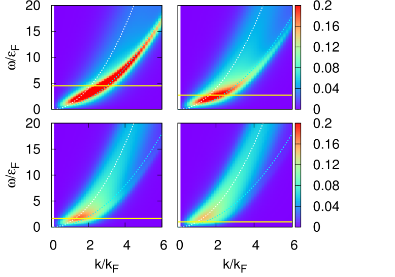
Figure 1: (color online) Color plot of the dynamical structure factor $S(\vec{q},\omega)$ (units $1/\varepsilon_{F}=(2m/\hbar^{2})(1/2\pi n)$) of a $2D$ Fermi gas for four values of the interaction parameter: $\log(k_{F}a)=0.0$ (top left panel), $0.5$ (top right panel), $1.0$ (bottom left panel) and $1.5$ (bottom right panel). We also show an horizontal line at $2|\Delta|$, the threshold to break Cooper pairs, the free atoms dispersion $e_{a}(q)=\hbar^{2}|\vec{q}|^{2}/2m$, and the free molecule dispersion $e_{m}(q)=\hbar^{2}|\vec{q}|^{2}/4m$.

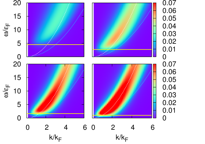
Figure 2: (color online) Color plot of the spin dynamical structure factor $S_{s}(\vec{q},\omega)$ (units $1/\varepsilon_{F}$) of a $2D$ Fermi gas. The setup is the same as in Fig. 1.

The results for the dynamical structure factor for the density $S(\vec{q},\omega)$ and the spin density $S_{s}(\vec{q},\omega)$ are shown in Figs. 1 and 2 respectively for four values of the interaction parameter, from the BEC regime $\log(k_{F}a)=0.0$ through to the BCS regime of $\log(k_{F}a)=1.5$.

At $\log(k_{F}a)=0.0$ the system is expected to behave as a gas of molecules. This is confirmed by the high momentum behavior $\hbar^{2}|\vec{q}|^{2}/2m>>|\Delta|$ of $S(\vec{q},\omega)$, where we have a spectrum of free molecules $S(\vec{q},\omega)\simeq\delta(\omega-e_{m}(\vec{q}))$, with $e_{m}(\vec{q})=\hbar^{2}|\vec{q}|^{2}/4m$ containing the mass of the molecules ($2m$). We observe that this behavior is not present is the spin structure factor $S_{s}(\vec{q},\omega)$: in order to create a modulation in spin density, it is necessary to first break a Cooper pair. This is the reason that the appreciable values for $S_{s}(\vec{q},\omega)$ lie above the line $2|\Delta|$, which is the estimated energy cost of breaking a molecule.

On the other side, in the BCS regime at $\log(k_{F}a)=1.5$ , the dynamical structure factors are more similar to the non-interacting results. The spectrum is centered around the free atom dispersion $e_{a}(\vec{q})=\hbar^{2}|\vec{q}|^{2}/2m$, with a broadening due to the particle-hole continuum.

We also see that the theory predicts a smooth interpolation between the two regimes, consistent with a BEC-BCS crossover. From comparison with AFQMC calculations, which we discuss next, it is seen that the results are in reasonably good agreement, although quantitative differences exist.

4 Quantum Monte Carlo Approach

Because of the mean-field nature of the approximations involved in dynamical BCS theory, it is not clear a priori how reliable the results are, especially in strongly interacting regimes. Quantum Monte Carlo (QMC) approaches provide an alternative. In particular, for the spin-balanced cold Fermi gas there is no fermion sign problem in the auxiliary-field Quantum Monte Carlo (AFQMC) method AFQMC-lecture-notes-2013 ; hubbard_benchmark ; PhysRevB.94.085103 ; PhysRevB.88.125132 . The AFQMC method is able to provide unbiased, numerically exact results for any observable on the ground state of the cold Fermi gas Hao-2DFG ; PhysRevA.84.061602 . We have recently showed ettoreGAP ; Ettore-2DFG that it is possible to reach beyond static properties and compute imaginary-time correlation functions such as

$$F(\vec{q},\tau)=\frac{1}{N}\frac{\langle\Psi_{0}|\,\hat{n}_{\vec{q}}\,e^{-\tau(\hat{H}-E_{0})}\,\hat{n}_{-\vec{q}}\,|\Psi_{0}\rangle}{\langle\Psi_{0}\,|\,\Psi_{0}\rangle}$$ (30)

where $N$ is the number of particles and $\hat{n}_{\vec{q}}$ the Fourier component of the density (or spin density) fluctuation operator. The exact zero-temperature relation:

$$F(\vec{q},\tau)=\int_{0}^{+\infty}d\omega e^{-\tau\omega}S(\vec{q},\omega)$$ (31)

allows us to then obtain predictions about the dynamical structure factor (density and spin density) of the system using analytic continuation techniques. In the following we will introduce the AFQMC method and discuss how to efficiently compute $F(\vec{q},\tau)$ for the Fermi gas system.

4.1 AFQMC formalism and static properties

We will introduce the basic notations of the methodology using the attractive Hubbard model Hamiltonian (4) in Sec. 2. The AFQMC methodology relies on the following AFQMC-lecture-notes-2013 :

$$|\,\Psi_{0}\rangle\propto\lim_{\beta\to+\infty}e^{-\beta(\hat{H}-E_{0})}|\phi_{T}\rangle\,,$$ (32)

where $E_{0}$ is an estimate of the ground state energy, and $|\phi_{T}\rangle$ a trial wave function which is not orthogonal to the many-body ground state $|\,\Psi_{0}\,\rangle$.

Trotter-Suzuki breakup together with Hubbard-Stratonovich transformation provides the following:

$$e^{-\beta(\hat{H}-E_{0})}=\left(e^{-\delta\tau(\hat{H}-E_{0})}\right)^{M}\simeq\left(\int d{\bf{x}}p({\bf{x}})\hat{B}({\bf{x}})\right)^{M}\,,$$ (33)

which becomes exact in the limit $M\to\infty$ ($\delta\tau=\beta/M$ is a time-step). At each time slice, there is one set of auxiliary-fields, ${\bf{x}}=(x_{1},\dots,x_{\mathcal{N}_{s}})$, which are a discrete set of Ising fields on the lattice. $\hat{B}({\bf{x}})$ is a one-particle propagator, and the function $p({\bf{x}})$ is a discrete probability density.

A key point of the methodology is that $\hat{B}(\bf{x})$ in Eq. (33), which is the result of the HS transformation, is the exponential of a one-body propagator; its application on a Slater determinant $|\phi\rangle$ results in another Slater determinant $|\phi^{\prime}\rangle$, given in matrix form by

$$\mathcal{B}(\bf{x})\Phi=\Phi^{\prime}\,,$$ (34)

where $\Phi=\Phi_{\uparrow}\otimes\Phi_{\downarrow}$, with $\Phi_{\sigma}$ being the $\mathcal{N}_{s}\times N_{\sigma}$ matrix containing the spin-$\sigma$ orbitals of the Slater determinant $|\phi\rangle$, and similarly for $|\phi^{\prime}\rangle$.

The standard path-integral AFQMC method allows us to evaluate ground state expectation values:

$$\langle\hat{O}\rangle=\frac{\langle\Psi_{0}|\,\hat{O}\,|\Psi_{0}\rangle}{\langle\Psi_{0}\,|\,\Psi_{0}\rangle}$$ (35)

by casting them in the integral form:

$$\langle\hat{O}\rangle=\int d{\bf{X}}\,\mathcal{W}({\bf{X}})\,\mathcal{O}({\bf{X}})\,.$$ (36)

In Eq. (36), ${\bf X}=({\bf x}(1),\dots,{\bf x}(M))$ denotes a path in auxiliary-field space. Choosing the trial wave function $|\phi_{T}\rangle$ as a single Slater determinant and introducing the notation:

$$\langle\phi_{L}|\,=\langle\phi_{T}|\,\hat{B}({\bf x}(M))\dots\hat{B}({\bf x}(l))$$ (37)

and

$$|\phi_{R}\rangle=\hat{B}({\bf x}(l-1))\dots\hat{B}({\bf x}(1))\,|\phi_{T}\rangle\,,$$ (38)

we have:

$$\mathcal{W}({\bf{X}})\propto\,\langle\phi_{L}\,|\,\phi_{R}\rangle\,\prod_{i=1}^{M}p({\bf{x}}(i))\,,$$ (39)

while the estimator is

$$\mathcal{O}({\bf{X}})=\frac{\langle\phi_{L}|\,\hat{O}\,|\phi_{R}\rangle}{\langle\phi_{L}\,|\,\phi_{R}\rangle}\,.$$ (40)

For attractive interaction and $N_{\uparrow}=N_{\downarrow}$, $\mathcal{W}({\bf{X}})$ remains non-negative for all possible auxiliary-field path configurations. The calculation is sign-problem free, allowing us to obtain exact results. We use a Metropolis sampling of the paths, exploiting a force bias Hao-2DFG ; AFQMC-lecture-notes-2013 that allows high acceptance ratio in the updates. The infinite variance problem is eliminated with a bridge link approach Hao-inf-var .

4.2 Dynamical properties

The AFQMC methodology allows us to also compute dynamical correlation functions in imaginary-time at zero temperature:

$$f(\tau)=\frac{\langle\Psi_{0}|\,\hat{O}\,e^{-\tau(\hat{H}-E_{0})}\,\hat{O}^{\dagger}\,|\Psi_{0}\rangle}{\langle\Psi_{0}\,|\,\Psi_{0}\rangle}\,,$$ (41)

where $\hat{O}$ can be any operator. We will focus here on one-body operators such as the particle density or the spin density.

The imaginary-time propagator between the operators $\hat{O}$ and $\hat{O}^{\dagger}$ can be expressed using Eq. (33). We insert an extra segment to the path: a number $N_{\tau}=\tau/\delta\tau$ of time-slices, ${\bf\tilde{x}}(1),\dots,{\bf\tilde{x}}(N_{\tau})$. The static estimator in Eq. (40) is replaced by the following dynamical estimator:

$$f({\bf{X}},\tau)=\frac{\langle\phi_{L}|\,\hat{O}\,\hat{B}({\bf{\tilde{x}}}(N_{\tau}))\dots\hat{B}({\bf{\tilde{x}}}(1))\,\,\hat{O}^{\dagger}|\phi_{R}\rangle}{\langle\phi_{L}\,|\hat{B}({\bf{\tilde{x}}}(N_{\tau}))\dots\hat{B}({\bf{\tilde{x}}}(1))\,|\,\phi_{R}\rangle}\,.$$ (42)

Below we will write $\hat{B}_{i}$ instead of $\hat{B}({\bf\tilde{x}}(i))$ for notational simplicity.

Standard approaches assaad_prb ; hirsch-stable ; jel_dyn_method ; jel_dyn_method2 to evaluate the expression in Eq. (42) require computational cost of $\mathcal{O}(\mathcal{N}^{3}_{s})$. We have recently introduced an approach ettoreGAP which allows computation of the matrix elements of dynamical Green functions and (spin) density correlation functions with computational cost of $\mathcal{O}(\mathcal{N}_{s}\,N^{2})$. For dilute systems such as the ultracold Fermi gas that we are concerned with here, the number of particles is significantly smaller than the number of lattice sites, $N\ll\mathcal{N}_{s}$. The approach thus offers a significant advantage which enables us to reach the realistic limits. Since the estimator (42) is computed sampling the same probability distribution as for static properties (40), a finite imaginary time $\tau>0$ does not introduce any bias. We will now sketch the method, which explicitly propagates fluctuations during the random walk.

4.3 Two-body correlation functions

Let us focus on the estimator:

$$n({\bf{X}},\tau)=\frac{\langle\phi_{L}|\,\hat{n}_{j,\sigma^{\prime}}\,\hat{B}_{N_{\tau}}\dots\hat{B}_{1}\,\,\hat{n}_{i,\sigma}|\phi_{R}\rangle}{\langle\phi_{L}\,|\,\hat{B}_{N_{\tau}}\dots\hat{B}_{1}\,\,|\,\phi_{R}\rangle}$$ (43)

where, as usual, $\hat{n}_{i,\sigma}=\hat{c}^{\dagger}_{i,\sigma}\hat{c}_{i,\sigma}$ is the fermion spin-resolved density operator.

It is straightforward to show

$$\hat{n}_{i,\sigma}=\frac{e^{\hat{n}_{i,\sigma}}-1}{e-1}\,.$$ (44)

This implies that, if $|\phi_{R}\rangle=\hat{c}^{\dagger}_{|u_{1},\uparrow\rangle}\dots\hat{c}^{\dagger}_{|u_{N_{\uparrow}},\uparrow\rangle}\hat{c}^{\dagger}_{|v_{1},\downarrow\rangle}\dots\hat{c}^{\dagger}_{|v_{N_{\downarrow}},\downarrow\rangle}|0\rangle$, the numerator in Eq. (43) can be viewed as the propagation of two Slater determinants:

$$\hat{n}_{i,\uparrow}|\phi_{R}\rangle=\frac{|\phi^{\prime}_{R}(i)\rangle-|\phi_{R}\rangle}{e-1}$$ (45)

where:

$$|\phi_{R}^{\prime}(i)\rangle=\hat{c}^{\dagger}_{|e^{\hat{n}_{i,\uparrow}}u_{1},\uparrow\rangle}\dots\hat{c}^{\dagger}_{|e^{\hat{n}_{i,\uparrow}}u_{N_{\uparrow}},\uparrow\rangle}\hat{c}^{\dagger}_{|v_{1},\downarrow\rangle}\dots\hat{c}^{\dagger}_{|v_{N_{\downarrow}},\downarrow\rangle}|0\rangle\,.$$ (46)

Consequently, Eq. (43) can be broken into two pieces:

$$n({\bf{X}},\tau)=\frac{1}{e-1}\left(n_{1}({\bf{X}},\tau)-n_{2}({\bf{X}},\tau)\right)\,,$$ (47)

which can be expressed as:

$$n_{1}({\bf{X}},\tau)=\frac{\langle\phi_{L}|\,\hat{n}_{j,\sigma^{\prime}}\hat{B}\,\,|\phi^{\prime}_{R}(i)\rangle}{\langle\phi_{L}\,|\hat{B}\,\,|\,\phi^{\prime}_{R}(i)\rangle}\,\,\frac{\langle\phi_{L}|\,\hat{B}\,\,|\phi^{\prime}_{R}(i)\rangle}{\langle\phi_{L}\,|\hat{B}\,\,|\,\phi_{R}\rangle}$$ (48)

and

$$n_{2}({\bf{X}},\tau)=\frac{\langle\phi_{L}|\,\hat{n}_{j,\sigma^{\prime}}\hat{B}\,\,|\phi_{R}\rangle}{\langle\phi_{L}\,|\hat{B}\,\,|\,\phi_{R}\rangle}\,.$$ (49)

Both $n_{1}({\bf{X}},\tau)$ and $n_{2}({\bf{X}},\tau)$ can be calculated with straightforward manipulations of Slater determinants. The average of $n({\bf{X}},\tau)$ over an ensemble of paths in the configuration space of the auxiliary field provides the estimation of the density or spin-density imaginary time correlation function.

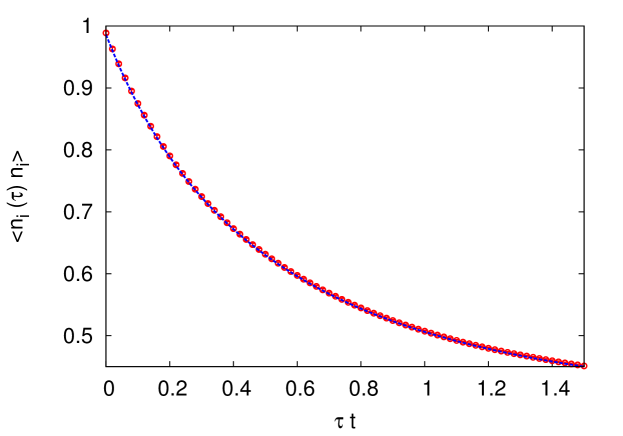
Figure 3: (color online) Imaginary-time on-site density-density correlation function $\langle\hat{n}_{i}\,e^{-\tau(\hat{H}-E_{0})}\,\hat{n}_{i}\rangle$ for the lattice Hamiltonian in Eq. (4) on a $4\times 4$ lattice hosting $10$ particles with $g_{\mathcal{L}}/t=4$. Comparison between the QMC computation (circles) and the exact diagonalization result (dotted line). AFQMC errors bars are shown but are smaller than symbol size.

In Fig. 3 we show a comparison between AFQMC and exact diagonalization results. We compute the same site density-density correlation in imaginary time for a $4\times 4$ lattice hosting $N=10$ particles with $g_{\mathcal{L}}/t=4$. Excellent agreement is seen, providing a strong calibration of the AFQMC algorithm.

5 Comparison between dynamical BCS theory and AFQMC

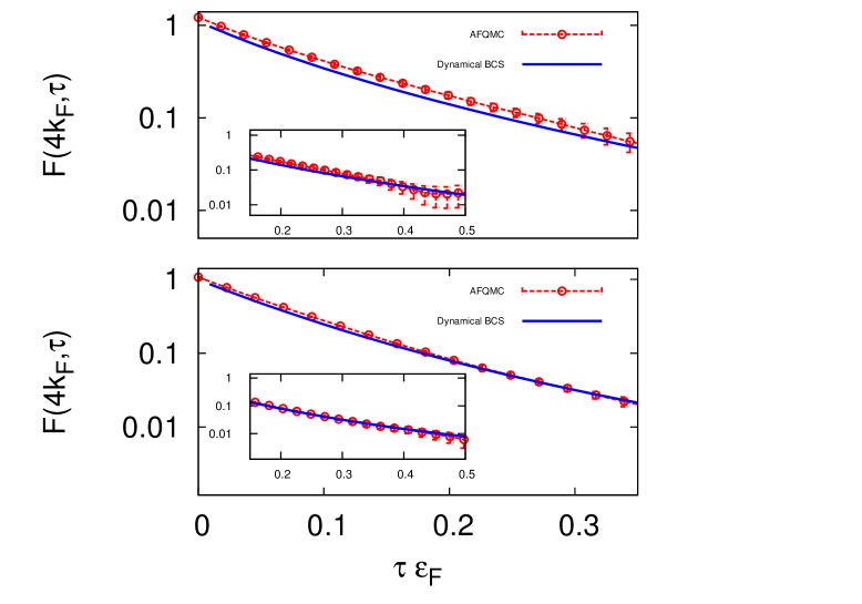
Figure 4: (color online) Comparison of imaginary-time density-density correlation, $F(\vec{q},\omega)$ at $q=4k_{F}$, obtained from dynamical BCS theory (blue full line) and AFQMC (red open circles). The top panel is in the crossover regime, at $\log(k_{F}a)=0.5$, while the bottom panel is in the BCS regime, at $\log(k_{F}a)=1.5$. The insets show the comparison for larger values of the imaginary time. The imaginary time window considered is large enough to capture the behavior of the density fluctuation mode at $q=4k_{F}$.

With the algorithm described above, we can compute unbiased imaginary-time correlation functions $F(\vec{q},t)$ for the 2D Fermi gas. The connection with dynamical structure factors is provided by the relation in Eq. (31), which has to be inverted to estimate $S(\vec{q},\omega)$. This is an analytic continuation problem, which can be delicate. However, a major advantage here is that the quality of the imaginary-time data is very high. State of art analytic continuation approaches have been shown to provide very accurate estimates under such circumstances, for instance in the realm of cold bosonic systems giftREV . A comprehensive study of the dynamical structure factors from AFQMC for the 2D gas will be presented elsewhere Ettore-2DFG .

Here we directly compare the result from dynamical BCS theory transformed into imaginary time domain with the exact AFQMC results. We stress that the direct Laplace transform, from frequency domain to imaginary time domain, can be performed with arbitrary accuracy, while the inverse transformation is much more challenging. In order to assess the quality of the dynamical BCS theory against unbiased AFQMC results, we choose a system of $N=18$ particles moving on a lattice with $25\times 25$ sites, and compute $F(\vec{q},t)$. We choose a high-momentum transfer of $q=4k_{F}$, which provides an interesting probe of the BCS-BEC crossover when the atomic spectrum evolves into the molecular spectrum.

In Fig. 4 we present the comparisons in the BCS regime and in the crossover regime. We see that, in the BCS regime at $\log(k_{F}a)=1.5$, dynamical BCS theory prediction is compatible with the exact result, except for a narrow window at small imaginary time, where all the excited states of the microscopic Hamiltonian play an important role. On the other hand, in the crossover regime at $\log(k_{F}a)=0.5$, the discrepancy is larger, although agreement is still restored in the large imaginary time region. This suggests that many-body correlations beyond dynamical mean field have important effects on response functions in the strongly-correlated BEC-BCS crossover. Considering sum rules, we observe that the $0$th moment, the static structure factor (that is the value of the correlation function at $\tau t=0$) is significantly different between the two approaches. On the other hand, the dynamical BCS theory strictly imposes the $1$st moment sum rule (”f sum rule”), which is also satisfied by the QMC result within statistical uncertainties.

Finally, we comment that the dynamical BCS theory calculations here provide a rigorous route to benchmark analytic continuation methods. By applying an analytic continuation method to the dynamical BCS data in the imaginary-time domain, one could directly compare the results against the corresponding results in the frequency domain. Together with the availability of exact AFQMC results in the imaginary-time domain here, the problem of the Fermi gas provides an excellent potential benchmark problem for methods to treat dynamical properties in strongly interacting many-fermion systems.

6 Conclusions

We have studied the response functions, and more precisely dynamical structure factors, of a two-dimensional cold gas with zero-range attractive interactions at zero-temperature. We computed $S(\vec{q},\omega)$ within the framework of dynamical BCS theory, which provides explicit approximate expressions involving integrals over momentum space. We also described an efficient algorithm to compute imaginary-time density and spin correlations with AFQMC for the dilute gases, and used the results to benchmark dynamical BCS theory.

The results of dynamical BCS theory show a spectrum of density fluctuations made of a fermionic particle-hole continuum superimposed to a gapless bosonic mode which, at high momentum, gives the response of a gas of free molecules on the BEC side of the crossover. The weight of such spectrum naturally decreases as we move towards the BCS regime, where the systems is similar to an ordinary superconductor.

The spin density fluctuation spectrum has a simpler structure. It displays a gap corresponding to the energy needed to break a Cooper pair, which is necessary to induce a spin density modulation at zero-temperature. At higher energies, the spectrum displays the typical particle-hole continuum.

We have discussed the importance and outlook of AFQMC calculations for imaginary-time correlations and response functions. Our AFQMC results are used to assess the accuracy of dynamical BCS theory. Discrepancies arise in the BEC-BCS crossover, although many qualitative features appear to be correctly described by dynamical BCS theory. Outside the strongly correlated regime, the theory is accurate and captures both the fermionic particle-hole excitations and the bosonic dynamics. The smaller differences in this regime tend to be more pronounced at shorter imaginary-times. A very interesting perspective will be the study of the possibility to use effective parametersPhysRevB.94.235119 in the dynamical BCS theory to improve the agreement with exact results.

- (1) P.A. Lee, N. Nagaosa, X.G. Wen, Rev. Mod. Phys. 78, 17 (2006). DOI 10.1103/RevModPhys.78.17. URL https://link.aps.org/doi/10.1103/RevModPhys.78.17
- (2) A.H. Castro Neto, F. Guinea, N.M.R. Peres, K.S. Novoselov, A.K. Geim, Rev. Mod. Phys. 81, 109 (2009). DOI 10.1103/RevModPhys.81.109. URL https://link.aps.org/doi/10.1103/RevModPhys.81.109
- (3) X.L. Qi, S.C. Zhang, Rev. Mod. Phys. 83, 1057 (2011). DOI 10.1103/RevModPhys.83.1057. URL https://link.aps.org/doi/10.1103/RevModPhys.83.1057
- (4) Y. Yu, A. Bulgac, Phys. Rev. Lett. 90, 161101 (2003). DOI 10.1103/PhysRevLett.90.161101. URL https://link.aps.org/doi/10.1103/PhysRevLett.90.161101
- (5) S. Giorgini, L.P. Pitaevskii, S. Stringari, Rev. Mod. Phys. 80, 1215 (2008). DOI 10.1103/RevModPhys.80.1215. URL http://link.aps.org/doi/10.1103/RevModPhys.80.1215
- (6) I. Bloch, J. Dalibard, W. Zwerger, Rev. Mod. Phys. 80, 885 (2008). DOI 10.1103/RevModPhys.80.885. URL http://link.aps.org/doi/10.1103/RevModPhys.80.885
- (7) V. Makhalov, K. Martiyanov, A. Turlapov, Phys. Rev. Lett. 112, 045301 (2014). DOI 10.1103/PhysRevLett.112.045301. URL https://link.aps.org/doi/10.1103/PhysRevLett.112.045301
- (8) M.G. Ries, A.N. Wenz, G. Zürn, L. Bayha, I. Boettcher, D. Kedar, P.A. Murthy, M. Neidig, T. Lompe, S. Jochim, Phys. Rev. Lett. 114, 230401 (2015). DOI 10.1103/PhysRevLett.114.230401. URL https://link.aps.org/doi/10.1103/PhysRevLett.114.230401
- (9) I. Boettcher, L. Bayha, D. Kedar, P.A. Murthy, M. Neidig, M.G. Ries, A.N. Wenz, G. Zürn, S. Jochim, T. Enss, Phys. Rev. Lett. 116, 045303 (2016). DOI 10.1103/PhysRevLett.116.045303. URL https://link.aps.org/doi/10.1103/PhysRevLett.116.045303
- (10) M. Feld, B. Frohlich, E. Vogt, M. Koschorreck, M. Kohl, Nature 480 (2011). DOI 10.1038/nature10627. URL http://dx.doi.org/10.1038/nature10627
- (11) C. Cheng, J. Kangara, I. Arakelyan, J.E. Thomas, Phys. Rev. A 94, 031606 (2016). DOI 10.1103/PhysRevA.94.031606. URL https://link.aps.org/doi/10.1103/PhysRevA.94.031606
- (12) M. Bauer, M.M. Parish, T. Enss, Phys. Rev. Lett. 112, 135302 (2014). DOI 10.1103/PhysRevLett.112.135302. URL http://link.aps.org/doi/10.1103/PhysRevLett.112.135302
- (13) L. He, H. Lü, G. Cao, H. Hu, X.J. Liu, Phys. Rev. A 92, 023620 (2015). DOI 10.1103/PhysRevA.92.023620. URL https://link.aps.org/doi/10.1103/PhysRevA.92.023620
- (14) M. Klawunn, Physics Letters A 380(34), 2650 (2016). DOI https://doi.org/10.1016/j.physleta.2016.06.015. URL http://www.sciencedirect.com/science/article/pii/S0375960116303206
- (15) A. Galea, H. Dawkins, S. Gandolfi, A. Gezerlis, Phys. Rev. A 93, 023602 (2016). DOI 10.1103/PhysRevA.93.023602. URL http://link.aps.org/doi/10.1103/PhysRevA.93.023602
- (16) G. Bertaina, S. Giorgini, Phys. Rev. Lett. 106, 110403 (2011). DOI 10.1103/PhysRevLett.106.110403. URL http://link.aps.org/doi/10.1103/PhysRevLett.106.110403
- (17) H. Shi, S. Chiesa, S. Zhang, Phys. Rev. A 92, 033603 (2015). DOI 10.1103/PhysRevA.92.033603. URL http://link.aps.org/doi/10.1103/PhysRevA.92.033603
- (18) E. Vitali, H. Shi, M. Qin, S. Zhang, ArXiv e-prints 1705.07929 (2017)
- (19) S. Hoinka, M. Lingham, M. Delehaye, C.J. Vale, Phys. Rev. Lett. 109, 050403 (2012). DOI 10.1103/PhysRevLett.109.050403. URL http://link.aps.org/doi/10.1103/PhysRevLett.109.050403
- (20) M.J. Stephen, Phys. Rev. 139, A197 (1965). DOI 10.1103/PhysRev.139.A197. URL https://link.aps.org/doi/10.1103/PhysRev.139.A197
- (21) O. Betbeder-Matibet, P. Nozieres, Ann. Phys. 51, 392 (1969). DOI 10.1016/0003-4916(69)90136-5. URL https://doi.org/10.1016/0003-4916(69)90136-5
- (22) R. Combescot, M.Y. Kagan, S. Stringari, Phys. Rev. A 74, 042717 (2006). DOI 10.1103/PhysRevA.74.042717. URL http://link.aps.org/doi/10.1103/PhysRevA.74.042717
- (23) E. Vitali, H. Shi, M. Qin, S. Zhang, Phys. Rev. B 94, 085140 (2016). DOI 10.1103/PhysRevB.94.085140. URL http://link.aps.org/doi/10.1103/PhysRevB.94.085140
- (24) P. Zou, F. Dalfovo, R. Sharma, X.J. Liu, H. Hu, New Journal of Physics 18(11), 113044 (2016). URL http://stacks.iop.org/1367-2630/18/i=11/a=113044
- (25) J. Carlson, S. Gandolfi, K.E. Schmidt, S. Zhang, Phys. Rev. A 84, 061602 (2011). DOI 10.1103/PhysRevA.84.061602. URL https://link.aps.org/doi/10.1103/PhysRevA.84.061602
- (26) F. Werner, Y. Castin, Phys. Rev. A 86, 013626 (2012). DOI 10.1103/PhysRevA.86.013626. URL http://link.aps.org/doi/10.1103/PhysRevA.86.013626
- (27) S. Zhang. Auxiliary-Field Quantum Monte Carlo for Correlated Electron Systems, Vol. 3 of Emergent Phenomena in Correlated Matter: Modeling and Simulation, Ed. E. Pavarini, E. Koch, and U. Schollwöck (Verlag des Forschungszentrum Jülich, 2013)
- (28) J.P.F. LeBlanc, A.E. Antipov, F. Becca, I.W. Bulik, G.K.L. Chan, C.M. Chung, Y. Deng, M. Ferrero, T.M. Henderson, C.A. Jiménez-Hoyos, E. Kozik, X.W. Liu, A.J. Millis, N.V. Prokof’ev, M. Qin, G.E. Scuseria, H. Shi, B.V. Svistunov, L.F. Tocchio, I.S. Tupitsyn, S.R. White, S. Zhang, B.X. Zheng, Z. Zhu, E. Gull, Physical Review X 5, 041041 (2015). DOI 10.1103/PhysRevX.5.041041. URL http://link.aps.org/doi/10.1103/PhysRevX.5.041041
- (29) M. Qin, H. Shi, S. Zhang, Phys. Rev. B 94, 085103 (2016). DOI 10.1103/PhysRevB.94.085103. URL https://link.aps.org/doi/10.1103/PhysRevB.94.085103
- (30) H. Shi, S. Zhang, Phys. Rev. B 88, 125132 (2013). DOI 10.1103/PhysRevB.88.125132. URL https://link.aps.org/doi/10.1103/PhysRevB.88.125132
- (31) H. Shi, S. Zhang, Phys. Rev. E 93, 033303 (2016). DOI 10.1103/PhysRevE.93.033303. URL http://link.aps.org/doi/10.1103/PhysRevE.93.033303
- (32) M. Feldbacher, F.F. Assaad, Phys. Rev. B 63, 073105 (2001). DOI 10.1103/PhysRevB.63.073105. URL http://link.aps.org/doi/10.1103/PhysRevB.63.073105
- (33) J.E. Hirsch, Phys. Rev. B 38, 12023 (1988). DOI 10.1103/PhysRevB.38.12023. URL http://link.aps.org/doi/10.1103/PhysRevB.38.12023
- (34) M. Motta, D.E. Galli, S. Moroni, E. Vitali, The Journal of Chemical Physics 140(2), 024107 (2014). DOI http://dx.doi.org/10.1063/1.4861227. URL http://scitation.aip.org/content/aip/journal/jcp/140/2/10.1063/1.4861227
- (35) M. Motta, D.E. Galli, S. Moroni, E. Vitali, The Journal of Chemical Physics 143(16), 164108 (2015). DOI http://dx.doi.org/10.1063/1.4934666. URL http://scitation.aip.org/content/aip/journal/jcp/143/16/10.1063/1.4934666
- (36) G. Bertaina, D.E. Galli, E. Vitali, Advances in Physics: X 2(2), 302 (2017). DOI 10.1080/23746149.2017.1288585. URL http://dx.doi.org/10.1080/23746149.2017.1288585
- (37) M. Qin, H. Shi, S. Zhang, Phys. Rev. B 94, 235119 (2016). DOI 10.1103/PhysRevB.94.235119. URL https://link.aps.org/doi/10.1103/PhysRevB.94.235119