Numerical simulation of surface brightness of astrophysical jets

We outline a general procedure for simulating the surface brightness of astrophysical jets (and other astronomical objects) by post-processing gas dynamical simulations of densities and temperatures using spectral line emission data from the astrophysical spectral synthesis package Cloudy. Then we validate the procedure by comparing the simulated surface brightness of the HH 30 astrophysical jet in the forbidden [O I], [N II], and [S II] doublets with Hubble Space Telescope observations of Hartigan and Morse and multiple-ion magnetohydrodynamic simulations of Tesileanu et al. The general trend of our simulated surface brightness in each doublet using the gas dynamical/Cloudy approach is in excellent agreement with the observational data.

1 Introduction

To understand the physics of astrophysical jets, especially near their sources, requires – in addition to densities, temperatures, and velocities – knowledge of surface brightness of the jets in different spectral lines. Simulated surface brightness maps in various lines may be constructed by applying gas dynamics or magnetohydrodynamics (MHD) with multiple ionic species and calculating the spectral emission from ionization effects in radiative cooling “on the fly,” as in the pioneering MHD computations of Tesileanu et al. (2014); or by applying gas dynamics (or MHD) with radiative cooling and then post-processing densities and temperatures using an astrophysical spectral synthesis package like Cloudy (version 13.03, last described by Ferland et al. 2013) to model the spectral emission (see Stute et al. (2010) for a very different application of this procedure, using a different set of software tools). In Gardner et al. 2016, surface brightness maps from our gas dynamics/Cloudy simulations of the SVS 13 micro-jet – traced by the emission of the shock excited 1.644 $\mu$m [Fe II] line – and bow shock bubble – traced in the lower excitation 2.122 $\mu$m H₂ line – projected onto the plane of the sky are shown to be in good qualitative agreement with (non-quantitative) observational images in these lines. This investigation will quantitatively compare simulated surface brightness results for the HH 30 jet of the more fundamental approach of Tesileanu et al. (2014) with our more phenomenological gas dynamics/Cloudy approach and with Hubble Space Telescope (HST) observations of Hartigan and Morse (2007).

The Herbig-Haro object HH 30 consists of a pair of jets from a young star in the Taurus star formation region at a distance of 140 pc (Kenyon et al. 1994). HST images display a nearly edge-on, flared, reflection nebula on both sides of an opaque circumstellar disk, with collimated jets emitted perpendicular to the disk on both sides and nearly in the plane of the sky (the declination angle is approximately 80^∘ with respect to the line of sight (Hartigan and Morse 2007)). The HH 30 jets extend out to about 0.25 pc from the stellar source in each direction (Lopez et al. 1996), but here we are concerned with the first 0.003 pc of the brighter (northeastern) blueshifted jet near its launch site. Since the nearly edge-on disk effectively blocks the stellar light, the jet can be studied as it emerges from the accretion disk.

We validate our gas dynamics/Cloudy procedure by comparing the simulated surface brightness of the HH 30 astrophysical jet in the forbidden [O I], [N II], and [S II] doublets with HST observations of Hartigan and Morse (2007) and simulations of Tesileanu et al. (2014). On a logarithmic scale, our surface brightness simulations along the center of the jet are always within $\pm 7.5$% of the observational data for all three doublets, and fit the observational data more tightly than the simulations of Tesileanu et al. (2014). (However, it is important to note that the aim of Tesileanu et al. (2014) was quite different: these authors simulated a generic MHD jet with radiative cooling and spectral emission from multiple ionic species, and then compared their generic simulation with the observational data from HH 30 and RW Aurigae.) More importantly, the general trend of our simulated surface brightness in each doublet closely follows the observational patterns, and we can simulate surface brightness all the way up to the circumstellar disk.

2 Numerical methods and radiative cooling

To simulate astrophysical jets, we apply the WENO (weighted essentially non-oscillatory) method (Shu 1999) – a modern high-order upwind method – to the equations of gas dynamics with atomic and molecular radiative cooling (see Ha et al. 2005, Gardner & Dwyer 2009, Gardner et al. 2016). The equations of gas dynamics with radiative cooling can be written as hyperbolic conservation laws for mass, momentum, and energy:

$$\frac{\partial\rho}{\partial t}+\frac{\partial}{\partial x_{i}}(\rho u_{i})=0$$ (1)

$$\frac{\partial}{\partial t}(\rho u_{j})+\frac{\partial}{\partial x_{i}}(\rho u_{i}u_{j})+\frac{\partial P}{\partial x_{j}}=0$$ (2)

$$\frac{\partial E}{\partial t}+\frac{\partial}{\partial x_{i}}\left(u_{i}(E+P)\right)=-C(n,T),$$ (3)

where $\rho=mn$ is the density of the gas, $m$ is the average mass of the gas atoms or molecules, $n$ is the number density, $u_{i}$ is the velocity, $\rho u_{i}$ is the momentum density, $P=nk_{B}T$ is the pressure, $T$ is the temperature, and $E$ is the energy density of the gas. Indices $i,\leavevmode\nobreak\ j$ equal 1, 2, 3, and repeated indices are summed over. The pressure is computed from the other state variables by the equation of state:

$$P=(\gamma-1)\left(E-\frac{1}{2}\rho u^{2}\right),$$ (4)

where $\gamma$ is the polytropic gas constant.

We use a “one fluid” approximation and assume that the gas is predominantly H above 8000 K, with the standard admixture of the most abundant elements in the interstellar medium (ISM); while below 8000 K, we assume the gas is predominantly H₂, with $n(H)/n(H_{2})\approx 0.01$. We make the further approximation that $\gamma$ equals $\frac{5}{3}$ (the value for a monatomic gas) for simplicity.

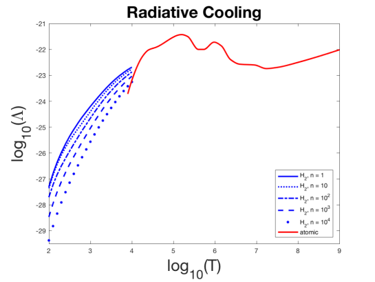
Figure 1: Atomic $\Lambda(T)$ and molecular $\Lambda(n,T)=W(n,T)/n$ cooling functions: $\log_{10}(\Lambda)$ with $\Lambda$ in erg cm³ s^-1, $n$ in H atoms/cm³ ($n$ = 100 corresponds to 50 H₂ molecules/cm³), and $T$ in K.

Radiative cooling (see Fig. 1) of the gas is incorporated through the right-hand side $-C(n,T)$ of the energy conservation equation (3), where

$$C(n,T)=\left\{\begin{array}[]{ll}n^{2}\Lambda(T)&T\geq 8000\leavevmode\nobreak\ {\rm K,\leavevmode\nobreak\ for\leavevmode\nobreak\ atomic\leavevmode\nobreak\ cooling\leavevmode\nobreak\ only}\\ nW(n,T)&T<8000\leavevmode\nobreak\ {\rm K,\leavevmode\nobreak\ for\leavevmode\nobreak\ H}_{2}\leavevmode\nobreak\ {\rm cooling\leavevmode\nobreak\ only}\\ \end{array}\right.$$ (5)

with the model for $\Lambda(T)$ taken from Fig. 8 of Schmutzler & Tscharnuter (1993) for atomic cooling, and the model for $W(n,T)$ from Fig. 4 of Le Bourlot et al. (1999) for H₂ molecular cooling. The atomic cooling model includes the relevant emission lines of the ten most abundant elements (H, He, C, N, O, Ne, Mg, Si, S, Fe) in the ISM, as well as relevant continuum processes. Both atomic and molecular cooling are actually operative between 8000 K $\leq T\leq$ 10,000 K, but atomic cooling is dominant in this range.

We use a positivity preserving (Hu et al. 2013) version of the third-order WENO method (Shu 1999, p. 439) for the gas dynamical simulations (Gardner et al. 2017). ENO and WENO schemes are high-order, upwind, finite-difference schemes devised for nonlinear hyperbolic conservation laws with piecewise smooth solutions containing sharp discontinuities like shock waves and contacts. Most numerical methods for gas dynamics can produce negative densities and pressures, breaking down in extreme circumstances involving very strong shock waves, shock waves impacting molecular clouds, strong vortex rollup, etc. By limiting the numerical flux, positivity preserving methods guarantee that the gas density and pressure always remain positive.

Below we calculate emission maps from the 2D cylindrically symmetric simulations of the HH 30 jet, at a distance of $R$ = 140 pc. To calculate the [O I] (6300 + 6363 Å), [N II] (6584 + 6548 Å), and [S II] (6716 + 6731 Å) doublet emission, we post-processed the computed solutions using emissivities $\epsilon(n,T)$ extracted and tabulated from Cloudy. In practice, we calculate (see Table 1) a table of values for $\log_{10}(\epsilon_{line})$ on a grid of $(\log_{10}(n),\log_{10}(T))$ values relevant in the simulations to each line, and then use bilinear interpolation in $\log_{10}(n)$ and $\log_{10}(T)$ to compute $\log_{10}(\epsilon_{line})$. For the simulations presented here, we calculated the emissivities for $2\leq\log_{10}(n)\leq 8$ with $n$ in H atoms/cm³ with a spacing of 0.1 in $\log_{10}(n)$; and for $3.8\leq\log_{10}(T)\leq 6$ with $T$ in K with a spacing of 0.05 in $\log_{10}(T)$.

Table 1: Cloudy code for calculating emissivities $\epsilon(n,T)$.

save grid ".grd"

c create ISM radiation field background

table ISM

abundances ISM

c vary Hydrogen density in powers of 10

hden 2 vary

grid 2 8 0.1

c vary temperature in powers of 10

constant temperature 3 vary

grid 3.8 6 0.05

c stop at zone 1 for speed

stop zone 1

c save emissivity

save lines emissivity ".ems"

O 1 6300A

O 1 6363A

N 2 6584A

N 2 6548A

c SII 6716A + 6731A:

S 2 6720A

end of lines

Surface brightness $S_{line}$ in any emission line is calculated by integrating along the line of sight through the jet and its surroundings

$$S_{line}=\frac{\int\epsilon_{line}(n,T)dl}{4\pi R^{2}}$$ (6)

where $R$ is the distance to the jet, and then converting to erg cm^-2 arcsec^-2 s^-1.

3 Results of numerical simulations

Parallelized cylindrically symmetric simulations were performed on a $750\Delta z\times 100\Delta r$ grid, spanning $1.5\times 10^{11}$ km by $0.4\times 10^{11}$ km (using the cylindrical symmetry). The jet was emitted through a disk-shaped inflow region in the $rz$ plane centered on the $z$-axis with a diameter of $10^{9}$ km, and propagated along the $z$-axis with an initial velocity of 300 km s^-1. The simulation parameters at $t=0$ for the jet and ambient gas are given in Table 2. The jet is propagating into previous outflows, so although the far-field ambient is lighter than the jet, the immediate ambient near the stellar source is likely to be nearly as dense as the jet itself. Further, the tapering morphology of the HST observations of the jet imply that the jet density is near the ambient density: if the jet is much heavier than the ambient, the jet would create a strong bow shock and would itself be wider; if the jet is much lighter than the ambient, the jet would also create a strong bow shock, plus strong Kelvin-Helmholtz rollup and entrainment of the ambient gas. Note that the jet and ambient gas are not pressure matched.

Table 2: Initial parameters for the jet and ambient gas.

Jet	Ambient Gas
$n_{j}$ = $10^{5}$ H/cm3	$n_{a}$ = $2.5\times 10^{4}$ H2/cm3
$u_{j}$ = 300 km s-1	$u_{a}$ = 0
$T_{j}$ = $10^{4}$ K	$T_{a}$ = $10^{3}$ K

The jet is periodically pulsed in order to approximate the observational density and temperature data in Hartigan and Morse (2007), with the pulse on for 6.5 yr and then off for 1.5 yr over the simulated time of 35 yr, giving four full pulses plus a final partial pulse. We then spatially match the partial pulse plus the next three full pulses of the jet (projected with a declination angle of 80^∘ with respect to the line of sight) out to $0.94\times 10^{11}$ km = 4.5 arcsec with the HST observations. Our approach was to vary the jet and ambient parameters and the pulses to obtain good agreement with the HST observations of density and temperature, and only then to calculate the surface brightness of the jet in the three forbidden doublets.

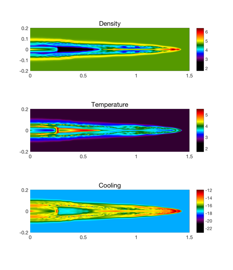
Figure 2: Logarithm of density $\log_{10}(n)$ with $n$ in H atoms/cm³ (top panel), logarithm of temperature $\log_{10}(T)$ with $T$ in K (middle panel), and logarithm of total radiative cooling $\log_{10}(C)$ with $C$ in erg cm^-3 s^-1 (bottom panel) at $t$ = 35 yr. Lengths along the boundaries are in units of $10^{11}$ km. The HST observations extend out to $0.94\times 10^{11}$ km = 4.5 arcsec.

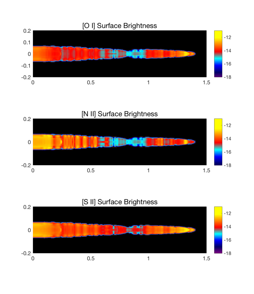
Figure 3: Simulated surface brightness $S$ in the [O I] (6300 + 6363 Å) doublet (top panel), [N II] (6584 + 6548 Å) doublet (middle panel), and [S II] (6716 + 6731 Å) doublet (bottom panel) at 35 yr, projected 80^∘ with respect to the line of sight: $\log_{10}(S)$ with $S$ in erg cm^-2 arcsec^-2 s^-1. Lengths along the boundaries are in $10^{11}$ km. The HST observations extend out to $0.94\times 10^{11}$ km = 4.5 arcsec.

In the simulation Figs. 2 and 3, the jet is surrounded by a thin bow shock plus thin bow-shocked cocoon. The jet is propagating initially at Mach 25 with respect to the sound speed in the jet/ambient gas. However, the jet tip actually propagates at an average velocity of approximately 110 km s^-1, at Mach 8 with respect to the average sound speed in the ambient gas, since the jet is slowed down as it impacts the ambient environment. The average velocity of gas within the jet is approximately 200 km s^-1, in excellent agreement with the HST observations (Bacciotti, et al. 1999).

The HH 30 jet is one of the densest jets observed (Bacciotti et al. 1999). Observationally the jet density starts at $10^{5}$ H/cm³, decreases to $5\times 10^{4}$ H/cm³ within first arcsec, and then gradually falls to $10^{4}$ H/cm³ at a few arcsec; the jet temperature starts at $2\times 10^{4}$  K, decreases to $10^{4}$ K within first arcsec, and then gradually decays to 6000–7000 K at a few arcsec. These data are well matched by our simulated densities and temperatures in Fig. 2 out to the limit of the HST observations at $0.94\times 10^{11}$ km = 4.5 arcsec.

Figure 3 presents our simulated surface brightness of the jet in the three forbidden doublets, projected onto the plane of the sky. The surface brightness has been smoothed with a Gaussian point-spread function with a width of 0.1 arcsec. Qualitatively the simulations are similar to the observations of Hartigan and Morse (2007), but the real test is to compare surface brightness in each doublet along the center of the jet.

4 Discussion

As is evident in Figs. 2 and 3, the jet pulses create a series of shocked knots followed by rarefactions within the jet. In Fig. 2, the panels indicate shocked knots at $z\approx 0.25$, 0.8, 1.0, and $1.4\times 10^{11}$ km, with an incipient knot beginning at $z=0$. The incipient knot plus the next three knots correspond roughly to the N, A, B, C knots illustrated in Hartigan and Morse (2007), while the final knot is outside the spatial range of their observations. In our simulations, the jet creates a terminal Mach disk near the jet tip, which reduces the velocity of the jet flow to the flow velocity of the contact discontinuity at the leading edge of the jet. With radiative cooling, the jet exhibits a higher density contrast near its tip (when the shocked, heated gas cools radiatively, it compresses), a narrower bow shock, and lower overall temperatures. There is a strong rarefaction between the knots for $z\approx 0.25$–$0.7\times 10^{11}$ km. The knots at $z\approx 0.25$, $0.8$, and $1.1\times 10^{11}$ km are undergoing especially strong radiative cooling. The temperature is highest around the knot at $z\approx 0.25$ and for the strong rarefaction between $z\approx 0.25$–$0.7\times 10^{11}$ km. In Fig. 3, there is strong cooling in all three doublets for $0\leq z\leq 0.6\times 10^{11}$ km and for $1.0\times 10^{11}\leq z\leq 1.4\times 10^{11}$ km. The [O I] doublet emission is low for $0.8\times 10^{11}\leq z\leq 1.0\times 10^{11}$ km, while the [N II] doublet emission is low for $0.7\times 10^{11}\leq z\leq 1.0\times 10^{11}$ km.

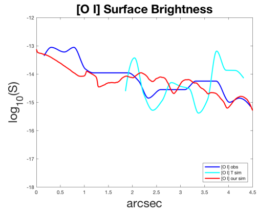
Figure 4: Logarithm of surface brightness $\log_{10}(S)$ in the [O I] (6300 + 6363 Å) doublet along the center of the projected jet, with $S$ in erg cm^-2 arcsec^-2 s^-1. Length scale is in arcsec from the source, with 1 arcsec = $0.21\times 10^{11}$ km.

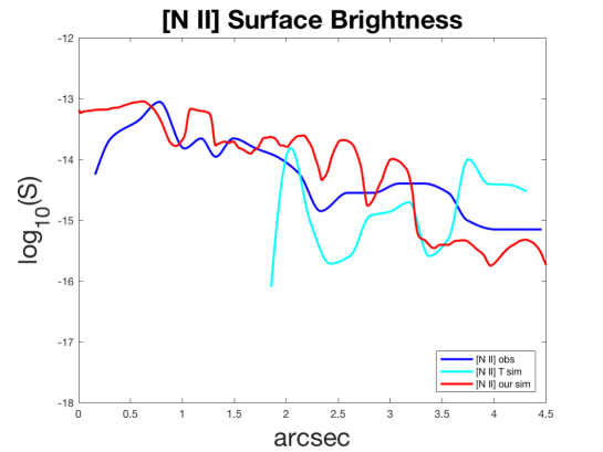
Figure 5: Logarithm of surface brightness $\log_{10}(S)$ in the [N II] (6584 + 6548 Å) doublet along the center of the projected jet, with $S$ in erg cm^-2 arcsec^-2 s^-1. Length scale is in arcsec from the source, with 1 arcsec = $0.21\times 10^{11}$ km.

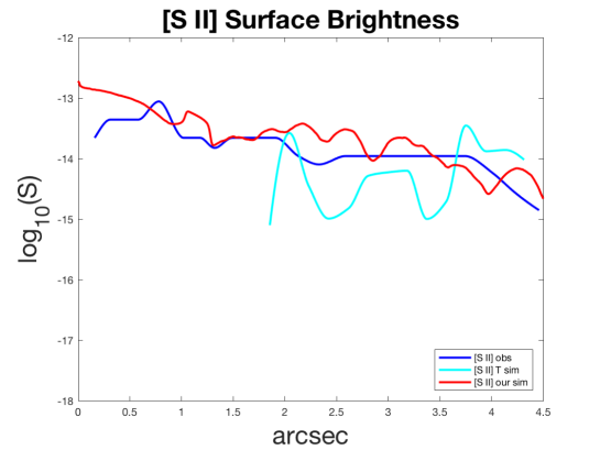
Figure 6: Logarithm of surface brightness $\log_{10}(S)$ in the [S II] (6716 + 6731 Å) doublet along the center of the projected jet, with $S$ in erg cm^-2 arcsec^-2 s^-1. Length scale is in arcsec from the source, with 1 arcsec = $0.21\times 10^{11}$ km.

Figures 4–6 present the comparisons of surface brightness in each of the three doublets along the center of the projected jet for observational data (labeled “obs”, from the data of Hartigan and Morse 2007), MHD multiple-ion simulations (labeled “T sim”, Tesileanu et al. 2014), and our gas dynamical/Cloudy simulations smoothed over 0.2 arcsec (labeled “our sim”). Our simulated surface brightness is within $\pm 7.5$% on the logarithmic scale of the observational data for the [O I], [S II], and [N II] forbidden doublets; in addition, the general trend of our simulated surface brightness maps closely follows the observational patterns from the limit of the HST data at 4.5 arcsec all the way up to the circumstellar disk.

5 Conclusion

The MHD simulations of Tesileanu et al. (2014) calculate radiative cooling and spectral emission using 19 ionic species: the first three ionization states (from I to III) of C, N, O, Ne, and S, as well as H I, H II, He I, and He II. Each additional ionic species significantly increases the computational complexity. Our atomic radiative cooling curve uses relevant ionization states of the first ten most abundant elements in the ISM, and is precomputed and tabulated: thus the computation of the jet evolution and cooling is computationally efficient. Emissivity in any spectral line in Cloudy can be pre-computed as a function of $\log_{10}(n)$ and $\log_{10}(T)$ and tabulated, and surface brightness in any line calculated as a post-processing step, which is also computationally efficient.

There are of course advantages to both approaches, and it is constructive to compare results of the two approaches. The approach of Tesileanu et al. (2014) is more fundamental, but our approach, while more phenomenological, is computationally much faster and can compute surface brightness in any molecular or atomic line incorporated into Cloudy. Further, simulating astrophysical jets with a gas dynamical solver with radiative cooling and then post-processing the simulated densities and temperatures with Cloudy produces simulated surface brightness maps that are in excellent agreement with the general progression of the observational data.

References

• Bacciotti, F., Eislöffel, J., & Ray, T. P. 1999, A&A 350, 917

• Ferland, G. J., Porter, R. L., van Hoof, P. A. M., et al. 2013, RMxAA, 49, 137

• Gardner, C. L., & Dwyer, S. J. 2009, AcMaS, 29B, 1677

• Gardner, C. L., Jones, J. R., & Hodapp, K. W. 2016, AJ, 830, 113

• Gardner, C. L., Jones, J. R., Scannapieco, E., & Windhorst, R. A. 2017, AJ, 835, 232

• Ha, Y., Gardner, C. L., Gelb, A., & Shu, C.-W. 2005, JSCom, 24, 29

• Hartigan, P., & Morse, J. 2007, AJ, 660, 426

• Hodapp, K. W., & Chini, R. 2014, ApJ, 794, 169

• Hu, X. Y., Adams, N. A., & Shu, C.-W. 2013, JCP, 242, 169

• Kenyon, S., Dobrzycka, D., & Hartmann, L. 1994, AJ, 108, 1872

• Krist, J. E., Stapelfeldt, K. R., Hester, J. J., et al. 2008, AJ, 136, 1980

• Le Bourlot, J., Pineau des Forêts, G., & Flower, D. R. 1999, MNRAS, 305, 802

• Lopez, R., Riera, A., Raga, et al. 1996, MNRAS, 282, 470

• Schmutzler, T., & Tscharnuter, W. M. 1993, A&A, 273, 318

• Shu, C.-W. 1999, High-Order Methods for Computational Physics, Vol. 9 (New York: Springer)

• Stute, M., Gracia, J., Tsinganos, K., Vlahakis, N. 2010, A&A, 516, A6

• Tesileanu, O., Matsakos, T., Massaglia, S., et al. 2014, A&A, 562, A117