Generalized Quasispecies Model on Finite Metric Spaces: Isometry Groups and Spectral Properties of Evolutionary Matrices

Abstract

The quasispecies model introduced by Eigen in 1971 has close connections with the isometry group of the space of binary sequences relative to the Hamming distance metric. Generalizing this observation we introduce an abstract quasispecies model on a finite metric space $X$ together with a group of isometries $\Gamma$ acting transitively on $X$. We show that if the domain of the fitness function has a natural decomposition into the union of $t$ $G$-orbits, $G$ being a subgroup of $\Gamma$, then the dominant eigenvalue of the evolutionary matrix satisfies an algebraic equation of degree at most $t\cdot{\rm rk}_{\mathbf{Z}}R$, where $R$ is what we call the orbital ring. The general theory is illustrated by two examples, in both of which $X$ is taken to be the metric space of vertices of a regular polytope with the “edge” metric; namely, the case of a regular $m$-gon and of a hyperoctahedron are considered.

Keywords:

Quasispecies model; finite metric space; dominant eigenvalue; mean population fitness; isometry group; regular polytope

AMS Subject Classification:

15A18; 92D15; 92D25

1 Introduction

The quasispecies model, initially put forward by Manfred Eigen in [11] to comprehensively study the problem of the origin of life, is now a classical object of modern evolutionary theory. More pertinent for the present paper, this model possesses a rich internal mathematical structure, as first was noted in [10, 20], where intriguing connections between evolutionary dynamics on sequence space and tensor products of representation spaces were pointed out. This mathematical framework, interesting on its own, facilitates understanding why some versions of Eigen’s model can be solved exactly and why for some other innocently looking versions numerical computations and subtle approximations are required. In [25] we noticed and used similar connections to introduce and analyze a special case of Eigen’s model, in which two different types of sequences are present; we also formulated, using geometric language, an abstract mathematical model, which we called the generalized quasispecies or Eigen model. The goal of this paper is to present in detail, expand, and elaborate on this generalized model with the ultimate objective to outline a proper mathematical framework in which many peculiarities of the Eigen model, including the notorious error threshold, can be understood from an algebraic point of view.

Eigen’s model is quite special in bringing together abstract mathematics and biology. Even more uniquely, it also has very tight connections with statistical mechanics. The complexity and richness of the original Eigen’s model can be emphasized by the fact that it is equivalent to the famous Ising model in statistical mechanics [18, 17]. The Ising model can be solved exactly only in some special cases, and hence any progress in understanding the conditions to solve Eigen’s model may yield insights in the analysis of the Ising model.

In what follows we neither aim for the most general formulation of the quasispecies model keeping the mutations symmetric and independent, nor we present the most abstract version of our model, using as the specific examples of the underlying metric spaces regular polytopes with natural “edge” metrics. In this way the presentation, in our opinion, can be accessible to theoretical biologists, physicists, and mathematicians alike. The rest of the text is organized as follows. In Section 2 we recall the classical Eigen’s model, provide a concise description of the main mathematical advances of its analysis and show in which way the hyperoctahedral group of isometries of the space of two-letter sequences with the Hamming distance naturally appears in the analysis of this model. This sets the stage for an abstract formulation of the generalized Eigen’s model on an arbitrary finite metric space in Section 3. In the same section we also review the necessary algebraic background and introduce what we call an orbital ring that allows identifying those spectral problems for which progress can be achieved. Section 4 contains an explicit equation for the dominant eigenvalue. In Section 5 we apply the abstract theory developed so far to two specific cases, namely, to the regular $m$-gon and to the hyperoctahedral mutational landscapes. Short Section 6 is devoted to the discussion of open problems and future directions. Finally, Appendix contains some additional calculations in a concise table form.

2 The quasispecies model

The quasispecies model [11, 12] is a system of ordinary differential equations that describes the changes with time of the vector of frequencies of different types of individuals in a population. To be specific, the individuals are defined to be sequences of a fixed length, say $N$, composed of a two-letter alphabet $\{0,1\}$, hence we have $2^{N}=:l$ different types of sequences. Sequences can reproduce and mutate; the former is incorporated into the diagonal matrix ${\boldsymbol{W}}=\operatorname{diag}(w_{0},\ldots,w_{l-1})$, which is called the fitness landscape, and the latter is described by the stochastic matrix ${\boldsymbol{Q}}$, which is called the mutation landscape. The entry $w_{i}\geq 0$ of ${\boldsymbol{W}}$ is the fitness of the sequence of type $i$, the entry $q_{ij}\in[0,1]$ of ${\boldsymbol{Q}}$ is interpreted as the probability that, upon reproduction, the sequence of type $j$ begets the sequence of type $i$. It is readily shown that the asymptotic state of the vector ${\boldsymbol{\hat{p}}}=(\hat{p}_{0},\ldots,\hat{p}_{l-1})^{\top}\in\mathbf{R}^{l}$ of frequencies of different types of sequences is the positive eigenvector corresponding to the dominant eigenvalue $\overline{w}$ of the eigenvalue problem

$${\boldsymbol{QW\hat{p}}}=\overline{w}{\boldsymbol{\hat{p}}}.$$ (2.1)

The dominant eigenvalue and the corresponding eigenvector exist under some very mild technical conditions on ${\boldsymbol{W}}$ and ${\boldsymbol{Q}}$ due to the Perron–Frobenius theorem. The leading eigenvalue $\overline{w}$ is called the mean population fitness and is given by $\overline{w}=\sum_{i=0}^{l-1}w_{i}\hat{p}_{i}$. (We note that there exists an equally popular evolutionary model, which is usually called the Crow–Kimura model, whose properties are close to the problem (2.1), see, e.g., [1, 4, 24]. Much more on the history and analysis of the various quasispecies models can be found in [1, 22, 15].)

To make further progress one needs to specify matrices ${\boldsymbol{W}}$ and ${\boldsymbol{Q}}$. In the simplest symmetric case we can assume that mutation at a given site of a sequence is independent from other mutations, and the mutation probability, which we denote $1-q$, such that $q$ is the fidelity, i.e., the probability of the error free reproduction, is the same for any site. Then

$$q_{ij}=q^{N-H_{ij}}(1-q)^{H_{ij}},\quad i,j=0,\ldots,l-1,$$

where $H_{ij}$ is the Hamming distance between sequences of types $i$ and $j$ (we use the lexicographical order to index the sequences, such that sequence $i$ is given by the binary representation of length $N$ of the integer $i$). Thus the model has the natural geometry of the binary hypercube $X=\{0,1\}^{N}$, see Fig. 2.1.

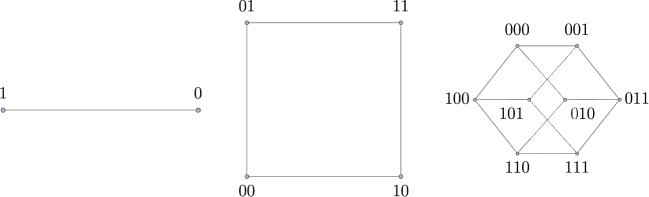
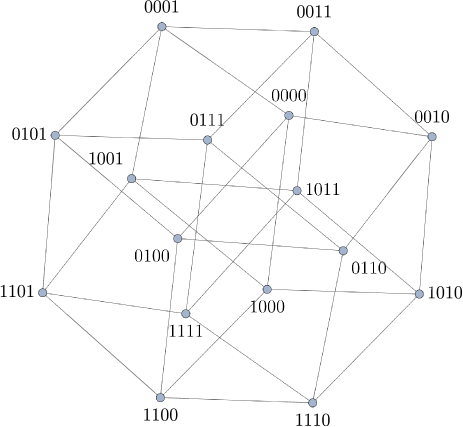
Figure 2.1: The underlying geometry of the classical Eigen’s model in the dimensions $N=1,2,3$ and $4$. The vertices correspond to different types of binary sequences, and the Hamming distance between two sequences is given by the minimal number of edges connecting them.

For matrix ${\boldsymbol{W}}$ it is possible to have different choices. One of the most frequently used is the so-called single peaked landscape (SPL), which is defined as

$${\boldsymbol{W}}_{SPL}:=\operatorname{diag}(w+s,w,\ldots,w),\quad w\geq 0,\,s>0.$$

It turns out that it is impossible, however, to calculate $\overline{w}$ and ${\boldsymbol{p}}$ exactly in this case for finite values of $N$, and the first analysis of the quasispecies model with SPL relied heavily on numerical calculations (see [27] and Fig. 2.2). Note that numerically it is not straightforward to solve the eigenvalue problem (2.1), even for moderate values of $N$, because the dimension of the matrices is $2^{N}\times 2^{N}$. To overcome this difficulty, Swetina and Schuster [27] considered only the so-called permutation invariant fitness landscapes whereas the fitness of a given sequence is determined by the Hamming distance from the master (zero) sequence. In this way one can track only the frequencies of class zero, which is the master sequence itself, of class one, which are all the sequences whose distance to the master sequence is one, etc, thus reducing the dimensionality of the problem to $(N+1)\times(N+1)$. SPL is an example of a permutation invariant fitness landscape.

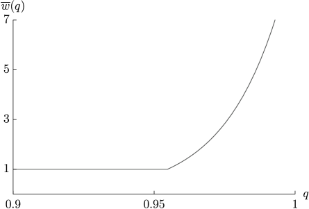
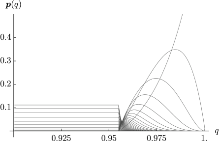
Figure 2.2: Numerical solution of the quasispecies model with the single peaked landscape. $N=50$, $w=1$, $s=9$. On the left the leading eigenvalue is shown, on the right the $y$-axis gives the frequencies of the sequences with the same Hamming distance from the master sequence.

Fig. 2.2 shows the phenomenon of the notorious error threshold: after some critical mutation rate the distribution of different types of sequences becomes uniform (and hence the distribution of classes shown in the right panel of Fig. 2.2 is binomial). We note that this phenomenon depends on the fitness landscape ${\boldsymbol{W}}$; for some ${\boldsymbol{W}}$ it does not manifest itself [15, 29, 30].

It turns out that it is possible to exactly calculate $\overline{w}$ and ${\boldsymbol{p}}$ for Eigen’s model in the case when the contributions to the overall fitness of different sites are independent [10, 20], and the mathematical reason for this is the decomposition of the Eigen evolutionary matrix ${\boldsymbol{QW}}$ as

$${\boldsymbol{QW}}={\boldsymbol{Q}}_{0}{\boldsymbol{W}}_{1}\otimes{\boldsymbol{Q}}_{0}{\boldsymbol{W}}_{3}\otimes\ldots\otimes{\boldsymbol{Q}}_{0}{\boldsymbol{W}}_{N},$$

where

$${\boldsymbol{Q}}_{0}=\begin{bmatrix}q&1-q\\ 1-q&q\\ \end{bmatrix},\quad{\boldsymbol{W}}_{k}=\begin{bmatrix}1&0\\ 0&s_{k}\\ \end{bmatrix},\quad k=1,\ldots,N,$$

$s_{k}$ is the contribution of the $k$-th site to the fitness, and $\otimes$ is the Kronecker product. Biologically, this case describes the absence of epistasis. More generally, as it was first noted in [10], the exact solution is in principle can be given if the structure of matrix ${\boldsymbol{W}}$ is related to the group of isometries of the binary hypercube $X=\{0,1\}^{N}$ (see also below).

Around the same time (at the end of 1980s) another major breakthrough about Eigen’s model was achieved: It was shown that the quasispecies model (2.1) is equivalent to the Ising model of statistical physics [18, 17], which actually caused a stream of papers that used methods of statistical physics to analyze (2.1) for various choices of ${\boldsymbol{W}}$ (see [3] and references therein). Without going into the details (see, e.g., [28] for an introduction to the Ising model), we mention that the Ising model is formulated for a given undirected graph, where the vertices can be in one of two states, and the edges represent the interactions between the vertices. In the classical two-dimensional Ising model that was solved by Onsager in 1944 [19] the graph is the lattice $\mathbf{Z}^{2}$. The solution is given in the limit when the number of vertices approaches infinity, and originally was obtained by analyzing the so-called transfer matrix, which, as was shown in [18, 17] is exactly equivalent to the evolutionary Eigen matrix ${\boldsymbol{QW}}$. Moreover, the error threshold in Eigen’s model is the phase transition in the Ising model.

Eventually the methods of statistical physics led to the maximum principle for the quasispecies model [2, 14] (see also [21]) that provides an efficient way of calculating the dominant eigenvalue $\overline{w}$ in the case of permutation invariant fitness landscapes and under some “continuity” condition on the limit of entries ${\boldsymbol{W}}$ when $N\to\infty$. Recently, the explicit expressions for the quasispecies distribution ${\boldsymbol{p}}$ for the permutation invariant fitness landscapes were obtained [7, 6].

Summarizing, we remark that, notwithstanding all the progress in the analysis of Eigen’s model (2.1) outlined above, there are a great deal of open questions. In particular, we still lack analytical tools to tackle “non-continuous” fitness landscapes (but see [25]), most of the existing approaches work only with permutation invariant landscapes, and there exist no necessary and sufficient conditions for the existence of the error threshold, to mention just a few. Most importantly, from our point of view, the existing analysis of Eigen’s model is almost exclusively concentrated on the case of the binary cube geometry (Fig. 2.1), which is supported by the biological motivation for the model (because the RNA and DNA molecules are literally polynucleotide sequences). Mathematically, however, nothing precludes us from considering an abstract model on a finite metric space $X$ with some natural metric, thus changing the mutational landscape of Eigen’s model. We introduced such abstract model in [25] and the rest of the present paper is devoted to a detailed presentation of this model and its analysis.

3 Generalized Eigen’s model and algebraic background

3.1 Groups of isometries and a generalized algebraic Eigen’s problem

Let $(X,d)$ be a finite metric space. We will assume that the metric $d\colon X\times X\longrightarrow\mathbf{N}_{0}$ is an integer-valued function. Consider a group $\Gamma\leqslant{\rm Iso}(X)$ of isometries of $X$ and suppose that $\Gamma$ acts transitively on $X$, that is, $X$ is a single $\Gamma$-orbit (we consider the left action).

Since $\Gamma$ acts transitively on $X$ we may fix an arbitrary point $x_{0}\in X$ and consider the function $d_{x_{0}}\colon X\longrightarrow\mathbf{N}_{0}$ such that $d_{x_{0}}(x)=d(x,x_{0})$. By definition,

$$\operatorname{diam}X:=\max\{d_{x_{0}}(x)\mid x\in X\}$$

is called the diameter of $X$. The number $N=\operatorname{diam}X$ does not depend on the choice of $x_{0}$.

Below we give two natural examples of such metric spaces. Arguably, the second example is mathematically more attractive, however, to keep a close connection to the classical Eigen’s model discussed in Section 2, the detailed calculations are presented for the metric spaces of more geometrically appealing Example 3.1.

Example 3.1 (Regular polytopes).

Let $X$ be the the set of vertices of an $n$-dimensional regular polytope $P$ (see, e.g., [8]), all edges of which have an integer length $e$. For example we can consider a regular $m$-gon ($m\geq 3$) on the plane, a tetrahedron, cube, octahedron, dodecahedron, or icosahedron in the 3-dimensional space (see Fig. 3.1) and so on, equipped with the “edge” metric: the distance between $x$ and $y$ is the minimal number of edges of $P$ connecting $x$ and $y$ multiplied by $e$. For the $n$-dimensional unit cube the edge metric is the same as the Hamming metric.

The full group of isometries $\Gamma={\rm Iso}(P)$ acts on $P$ and, consequently, on $X$. For instance, let $P$ be an icosahedron or dodecahedron. Then $\Gamma\cong A_{5}$ where $A_{5}<S_{5}$ is the alternating group of order 60.

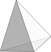
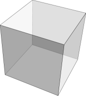
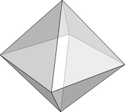
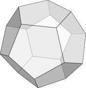
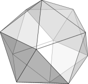
Figure 3.1: Platonic solids (examples of regular polytopes) in dimension 3. From left to right: tetrahedron (regular simplex), cube, octahedron, dodecahedron, icosahedron.

Example 3.2 (Groups as metric spaces).

Let $G$ be a finite group generated by a set $S=S^{-1}$. The word metric $d=d_{S}$ on $G$ is defined as follows (see [9, chapter IV ] for more details and examples): $d(g,h)=l(g^{-1}h)$ where $l(g^{-1}h)=l$ is the minimal number of generators $s\in S$ needed to represent $g^{-1}h$ as a product $s_{1}\dots s_{l}$. The word metric is invariant with respect to the action of $G$ on itself by left shifts $h\mapsto gh$. Hence, we have the metric space $X=G$ and the transitive action of $\Gamma=G$ on $X$ by isometries.

More generally, for any subgroup $H<G$ we can define the metric space $X_{H}=\{gH\,|\,g\in G\}$ of the left cosets of $G$ by $H$. The group $G$ acts on $X_{H}$ by left shifts and

$$d(gH,aH)=\min\{d(x,y)\mid x\in gH,\,y\in aH\}\,.$$

If $G$ acts transitively by isometries on a metric space $X$ then as a $G$-set $X$ is isomorphic to the set of left cosets $G/{\rm St}_{\Gamma}(x_{0})$, $x_{0}\in X$, where ${\rm St}_{\Gamma}(x_{0})$ is the stabilizer (or the group of isotropy) of $x_{0}$ in $\Gamma$.

Now consider a quadruple $(X,d,\Gamma,{{\boldsymbol{w}}})$ where $(X,d)$ is a finite metric space of diameter $N$ with integer distances between points and cardinality $l=|X|$, a group $\Gamma\leqslant{\rm Iso}(X)$ is a fixed group and a fitness function ${{\boldsymbol{w}}}\colon X\longrightarrow\mathbf{R}_{\geq 0}$. The fitness function is often represented by the vector-column ${{\boldsymbol{w}}}=(w_{x})$ with non-negative real entries called fitnesses which are indexed by $x\in X$ (for an appropriate ordering of $X$).

Definition 3.3.

The quadruple $(X,d,\Gamma,{{\boldsymbol{w}}})$ is called homogeneous $\Gamma$-landscape. It is called symmetric if for any points $y,z\in X$ there is an isometry $\gamma=\gamma(y,z)\in\Gamma$ such that $\gamma y=z$ and $\gamma z=y$.

Consider also the diagonal matrix ${{\boldsymbol{W}}}={\rm diag}(w_{x})$ of order $l$ called the fitness matrix, the symmetric distance matrix ${{\boldsymbol{D}}}=\bigl{(}d(x,y)\bigr{)}$ of the same order with integer entries, and the symmetric matrix ${{\boldsymbol{Q}}}=\left((1-q)^{d(x,y)}q^{N-d(x,y)}\right)$ for $q\in[0,1]$. Finally, we introduce the distance polynomial

$$P_{X}(q)=\sum_{x\in X}(1-q)^{d(x,x_{0})}q^{N-d(x,x_{0})}\,,\quad x_{0}\in X\,.$$ (3.1)

Since $\Gamma$ acts transitively on $X$ this polynomial is independent of the choice of $x_{0}\in X$ and is the sum of entries in each row (column) of ${{\boldsymbol{Q}}}$.

The following key definition generalizes the classical Eigen’s problem.

Definition 3.4.

The problem to find the leading eigenvalue $\overline{w}=\overline{w}(q)$ of the matrix $\frac{1}{P_{X}(q)}\,{\boldsymbol{QW}}$ and the eigenvector ${\boldsymbol{\hat{p}}}={\boldsymbol{\hat{p}}}(q)$ satisfying

$${{\boldsymbol{Q}}}{{\boldsymbol{W}}}{\boldsymbol{\hat{p}}}=P_{X}(q)\overline{w}\,{\boldsymbol{\hat{p}}},\quad\hat{p}_{x}=\hat{p}_{x}(q)>0,\quad\sum_{x\in X}\hat{p}_{x}(q)=1,$$ (3.2)

will be called generalized algebraic quasispecies or Eigen’s problem.

Note that in (3.2)

$$\overline{w}=\sum_{x\in X}w_{x}\hat{p}_{x}\,.$$ (3.3)

Due to the Perron–Frobenius theorem a solution of this problem always exists. Also note that the uniform distribution vector

$${\boldsymbol{\hat{p}}}=\frac{1}{|X|}(1,\dots,1)^{\top}=\frac{1}{l}(1,\dots,1)^{\top}$$ (3.4)

provides a solution of (3.2) in the case of constant fitnesses $w_{x}\equiv w>0$. By construction matrix $\frac{1}{P_{X}(q)}\,{{\boldsymbol{Q}}}$ is symmetric and double stochastic. It will be called generalized mutation matrix.

Problem (3.2) turns into classical Eigen’s quasispecies problem if $X=\{0,1\}^{N}$ is the $N$-dimensional binary cube with the Hamming metric $H$, and the group $\Gamma={\rm Iso}(X)$ named in 1930 by A. Young the hyperoctahedral group. $\Gamma$ is isomorphic as an abstract group to the Weyl group of the root system of type $B_{N}$ or $C_{N}$ and is acting on the binary cube. In this case $P_{X}(q)\equiv 1$. The case when $X$ is the set of vertices of an $N$-dimensional simplex with the isometry group ${\rm Iso}(X)\cong S_{n+1}$ is treated in detail in Section 6 of [25]. Here we continue with a general analysis of the generalized quasispecies problem. The first step is to study the properties of the distance polynomials.

3.2 Some general properties of the distance polynomial

Using the notations of Section 3.1 we consider the polynomial $P_{X}(q)=P_{X,d}(q)$. Polynomial $P_{X}(q)$ is strictly positive on $[0,1]$ (provided the parameter $N$ is strictly equal to $\operatorname{diam}X$) and possesses the following properties, which are checked by direct calculations:

1. $$P_{X}(1)=1,\quad P_{X}\left(\frac{1}{2}\right)=\frac{|X|}{2^{N}}=\frac{l}{2^{N}}\;.$$ (3.5)

2. $$P_{X}(q)=\sum_{k=0}^{N}f_{k}\,(1-q)^{k}q^{N-k}\in\mathbf{Z}[q]\,,$$ (3.6)

   where the non-negative integers $f_{k}=f_{k}(X)=:\#\{x\in X\mid d(x,x_{0})=k\}$ are the cardinalities of $d$-spheres in $X$ with the center at the fixed point $x_{0}$ and of radius $k$.

Remark 3.5.

Polynomial $S_{X}(t)=\sum_{k=0}^{N}f_{k}t^{k}$ is often called the spherical growth function of $(X,d)$. See, for instance, [9, chapter IV ] for details and examples.

3.3 An orbital ring associated with the triple $(X,d,\Gamma)$

In this section, to study the spectral properties of the mutation matrix ${\boldsymbol{Q}}$, we introduce what we call an orbital ring. For more algebraic details and construction of similar structures we refer the reader to [5, 13, 16, 23, 26].

Specifically, let $(X,d,\Gamma,{{\boldsymbol{w}}})$ be a homogeneous symmetric (in the sense of Definition 3.3) $\Gamma$-landscape ($\Gamma\leqslant{\rm Iso}(X)$). We attach to the triple $(X,d,\Gamma)$ a commutative ring $R=R(X,d,\Gamma)$ with unity, which we call the orbital ring. As an abelian group $R$ is free and of rank ${\rm rk}_{\mathbf{Z}}R=|\Gamma_{0}\backslash\Gamma/\Gamma_{0}|$, the number of double $(\Gamma_{0},\Gamma_{0})$-cosets in $\Gamma$ where $\Gamma_{0}={\rm St}_{\Gamma}(x_{0})$.

Since $\Gamma$ acts by isometries on $X$ then the distance function $d=d(x,y)$ is $\Gamma$-invariant with respect to the diagonal action of $\Gamma$ on the cartesian square $X\times X$, namely, $d(\gamma x,\gamma y)=d(x,y)$ for any $x,y\in X$ and $\gamma\in\Gamma$.

Let $A$ be a $\Gamma$-orbit in $X\times X$ and let ${{\boldsymbol{M}}}_{A}$ be the matrix with entries $({{\boldsymbol{M}}}_{A})_{x,y}$ equal to 1 if $(x,y)\in A$ and equal to 0 otherwise. It is worth mentioning that ${{\boldsymbol{M}}}_{A}$ can be identified with the matrix of $\Gamma$-invariant $\mathbf{Z}$-linear endomorphism $f_{A}\in{\rm Hom}(\mathbf{Z}X,\mathbf{Z}X)$ such that $f_{A}(y)=\sum_{(x,y)\in A}x$, $\mathbf{Z}X$ being a permutation $\mathbf{Z}\Gamma$-module (see, e.g., [5]).

It is well known that the set ${\rm Orb}$ of $\Gamma$-orbits $A$ in $X\times X$ is in 1-to-1 correspondence with the set $\Gamma_{0}\backslash\Gamma/\Gamma_{0}$ of double $(\Gamma_{0},\Gamma_{0})$-cosets in $\Gamma$ where $\Gamma_{0}={\rm St}_{\Gamma}(x_{0})$. We will say that $\Gamma$-orbit $A$ is of degree $k$ ($\deg A=k$), $k=0,\dots,N$, if $d(x,y)=k$ for some (and hence for any) $(x,y)\in A$. By definition, all $\Gamma$-orbits $A$ of degree $k$ compose a subset ${\rm Orb}_{k}\subset{\rm Orb}$.

Note that the single $\Gamma$-orbit of degree 0 is the diagonal $\Delta\subset X\times X$. The corresponding matrix ${{\boldsymbol{M}}}_{\Delta}={{\boldsymbol{I}}}$, the identity matrix. Since different orbits $A$ are disjoint the matrices ${{\boldsymbol{M}}}_{A}$ are independent over $\mathbf{Z}$.

Therefore, we have the following expansion of the mutation matrix ${{\boldsymbol{Q}}}$:

$${{\boldsymbol{Q}}}=\sum_{k=0}^{N}(1-q)^{k}q^{N-k}\sum_{A\in{\rm Orb}_{k}}{{\boldsymbol{M}}}_{A}\,,$$ (3.7)

and the equality

$${{\boldsymbol{E}}}=\sum_{A\in{\rm Orb}}{{\boldsymbol{M}}}_{A}=\sum_{k=0}^{N}\sum_{A\in{\rm Orb}_{k}}{{\boldsymbol{M}}}_{A}\,,$$ (3.8)

where ${{\boldsymbol{E}}}$ is the matrix with all the entries equal to 1.

Lemma 3.6.

If the triple $(X,d,\Gamma)$ is symmetric in the sense of Definition 3.3 then matrices ${{\boldsymbol{M}}}_{A}$ are symmetric and commute pairwise. Moreover, there are integer non-negative structural constants $\mu_{AB}^{C}=\mu_{BA}^{C}$, where $A,B,C\in{\rm Orb}$, such that

$${{\boldsymbol{M}}}_{A}{{\boldsymbol{M}}}_{B}=\sum_{C\in{\rm Orb}}\mu_{AB}^{C}{{\boldsymbol{M}}}_{C}\,.$$ (3.9)

Proof.

Let $(x,z)\in A$. In view of Definition 3.3 there exists an isometry $\gamma=\gamma(x,z)\in\Gamma$ such that $\gamma x=z$ and $\gamma z=x$. Thus, $(z,x)\in A$ and ${{\boldsymbol{M}}}_{A}$ is symmetric.

Moreover, it follows from the definition that for any $x,z\in X$ the corresponding matrix entry

$$({{\boldsymbol{M}}}_{A}{{\boldsymbol{M}}}_{B})_{x,z}=\#\{y\in X\mid(x,y)\in A,\;(y,z)\in B\}\,.$$ (3.10)

On the other hand, for the same transposing isometry $\gamma=\gamma(x,z)\in\Gamma$

$$\#\{y\in X\mid(x,y)\in A,\;(y,z)\in B\}=\#\{y\in X\mid(z,y)\in B,\;(y,x)\in A\}=$$

$$=\#\{\gamma y\in X\mid(\gamma z,\gamma y)\in B,\;(\gamma y,\gamma x)\in A\}=\#\{\gamma y\in X\mid(x,\gamma y)\in B,\;(\gamma y,z)\in A\}\,.$$

It follows that $({{\boldsymbol{M}}}_{A}{{\boldsymbol{M}}}_{B})_{x,z}=({{\boldsymbol{M}}}_{B}{{\boldsymbol{M}}}_{A})_{x,z}$ and ${{\boldsymbol{M}}}_{A}{{\boldsymbol{M}}}_{B}={{\boldsymbol{M}}}_{B}{{\boldsymbol{M}}}_{A}$.

The pair $(x,z)$ defines a $\Gamma$-orbit $C$. For $g\in\Gamma$ we have the same as in (3.10) non-negative number

$$({{\boldsymbol{M}}}_{A}{{\boldsymbol{M}}}_{B})_{gx,gz}=\#\{gy\in X\mid(gx,gy)\in A,\;(gy,gz)\in B\}\,.$$

Hence, (3.9) holds for some non-negative integer constants $\mu_{AB}^{C}$. The lemma is proved. ∎

Consequently, we have proved

Theorem 3.7.

All $\mathbf{Z}$-linear combinations of ${{\boldsymbol{M}}}_{A}$, $A\in{\rm Orb}$, compose a commutative unital ring $R=R(X,d,\Gamma)$ with unity ${{\boldsymbol{M}}}_{\Delta}={{\boldsymbol{I}}}$ called the orbital ring associated with the symmetric triple $(X,d,\Gamma)$. As $\mathbf{Z}$-module $R$ is free of rank ${\rm rk}_{\mathbf{Z}}R=|{\rm Orb}|=|\Gamma_{0}\backslash\Gamma/\Gamma_{0}|$.

Example 3.8.

Let $X=\{0,1\}^{2}$ be the binary square with points $x_{0}=[0,0]$, $x_{1}=[0,1]$, $x_{2}=[1,0]$, $x_{3}=[3,1]$ (binary representation of indices) with the Hamming metric $d$. Let $\Gamma\cong D_{4}$ (the dihedral group of order 8) be the group of all isometries of $X$. Then the triple $(X,d,\Gamma)$ is symmetric.

The set ${\rm Orb}$ consists of three orbits (corresponding to the three orbits, namely, $d$-spheres $\{x_{0}\}=S_{0}(x_{0})$, $\{x_{1},x_{2}\}=S_{1}(x_{0})$, $\{x_{3}\}=S_{2}(x_{0})$, of the stabilizer $\Gamma_{0}={\rm St}_{\Gamma}(x_{0})\cong\mathbf{Z}/2\mathbf{Z}$ acting on $X$) represented by matrices

$${{\boldsymbol{M}}_{0}}={{\boldsymbol{I}}}=\left[\begin{array}[]{cccc}1&0&0&0\\ 0&1&0&0\\ 0&0&1&0\\ 0&0&0&1\\ \end{array}\right]\,,\quad{{\boldsymbol{M}}_{1}}=\left[\begin{array}[]{cccc}0&1&1&0\\ 1&0&0&1\\ 1&0&0&1\\ 0&1&1&0\\ \end{array}\right]\,,\quad{{\boldsymbol{M}}_{2}}=\left[\begin{array}[]{cccc}0&0&0&1\\ 0&0&1&0\\ 0&1&0&0\\ 1&0&0&0\\ \end{array}\right]\,.$$

The multiplication table of these matrices in $R=R(X,d,\Gamma)$ is as follows:

$$\begin{array}[]{|c||c|c|c|}\hline\cr\times&{{\boldsymbol{I}}}&{{\boldsymbol{M}}_{1}}&{{\boldsymbol{M}}_{2}}\\ \hline\cr{{\boldsymbol{I}}}&{{\boldsymbol{I}}}&{{\boldsymbol{M}}_{1}}&{{\boldsymbol{M}}_{2}}\\ \hline\cr{{\boldsymbol{M}}_{1}}&{{\boldsymbol{M}}_{1}}&2{{\boldsymbol{I}}}+2{{\boldsymbol{M}}_{2}}&{{\boldsymbol{M}}_{1}}\\ \hline\cr{{\boldsymbol{M}}_{2}}&{{\boldsymbol{M}}_{2}}&{{\boldsymbol{M}}_{1}}&{{\boldsymbol{I}}}\\ \hline\cr\end{array}$$

Remark 3.9.

We have not yet applied the triangle inequality $d(x,z)\leq d(x,y)+d(y,z)$. It can be used for the construction of a graded ring ${\rm gr}\,R={\rm gr}\,R(X,d,\Gamma)$. Consider the following increasing filtration on $R$:

$$R_{-1}=0<\mathbf{Z}=R_{0}<R_{1}<\dots<R_{N}=R\,\quad\mbox{for $\mathbf{Z}$-modules}\;\;R_{k}=\bigoplus_{{\rm deg}A\leq k}\mathbf{Z}{{\boldsymbol{M}}}_{A}\,.$$

It follows from the definition and the triangle inequality that $R_{i}\cdot R_{j}\subseteq R_{i+j}$. Hence, we can attach to the triple $(X,d,\Gamma)$ the graded ring

$${\rm gr}\,R=\bigoplus_{k=0}^{N}R_{k}/R_{k-1}\,.$$

For instance, in the above Example 3.8 (here ${{\boldsymbol{M}}}_{k}\in{\rm gr}_{k}R=R_{k}/R_{k-1}$ is viewed as the corresponding element of $R_{k}$ modulo $R_{k-1}$):

$$\begin{array}[]{|c||c|c|c|}\hline\cr\times&{{\boldsymbol{I}}}&{{\boldsymbol{M}}_{1}}&{{\boldsymbol{M}}_{2}}\\ \hline\cr{{\boldsymbol{I}}}&{{\boldsymbol{I}}}&{{\boldsymbol{M}}_{1}}&{{\boldsymbol{M}}_{2}}\\ \hline\cr{{\boldsymbol{M}}_{1}}&{{\boldsymbol{M}}_{1}}&2{{\boldsymbol{M}}_{2}}&0\\ \hline\cr{{\boldsymbol{M}}_{2}}&{{\boldsymbol{M}}_{2}}&0&0\\ \hline\cr\end{array}$$

3.4 Spectral properties of the mutation matrix ${\boldsymbol{Q}}$

Consider now the space $V={\rm Hom}_{\mathbf{R}}(X,\mathbf{R})$ of all linear functions $f\colon X\longrightarrow\bf R$. Each function of $V$ can be represented as a vector-column ${{\boldsymbol{v}}}=(f(x))$ (in fact, a covector). The matrix ${{\boldsymbol{M}}}_{A}$ (see the previous section for the definition) defines a linear endomorphism ${{\boldsymbol{M}}}_{A}:V\longrightarrow V$ such that

$${{\boldsymbol{M}}}_{A}f(x)=\sum_{y\colon(x,y)\in A}f(y)\,.$$

If ${{\boldsymbol{v}}}=(f(x))$ then this endomorphism is just the multiplication ${{\boldsymbol{v}}}\mapsto{{\boldsymbol{M}}}_{A}{{\boldsymbol{v}}}$.

Let us show that each endomorphism ${{\boldsymbol{M}}}_{A}$ commutes with $\Gamma$-action on $V={\rm Hom}_{\mathbf{R}}(X,\mathbf{R})$ given by the rule $\gamma f(x)=f(\gamma^{-1}x)$, $\gamma\in\Gamma$. In fact,

$$\gamma{{\boldsymbol{M}}}_{A}f(x)={{\boldsymbol{M}}}_{A}f(\gamma^{-1}x)=\sum_{y:\,(\gamma^{-1}x,y)\in A}\!\!\!f(y)=\sum_{y:\,(x,\gamma y)\in A}\!\!\!f(y)=\sum_{z:\,(x,z)\in A}\!\!\!f(\gamma^{-1}z)={{\boldsymbol{M}}}_{A}\gamma f(x)\,.$$ (3.11)

Theorem 3.10.

Let the triple $(X,d,\Gamma)$ be symmetric. Then there exists a non-degenerate real constant transition matrix ${{\boldsymbol{T}}}=(t_{x,y})$ of order $l=|X|$ such that

1. All matrix entries of ${{\boldsymbol{T}}}$ are integer algebraic (over the field $\mathbf{Q}$) numbers.
   

2. The column of ${{\boldsymbol{T}}}$ indexed by a fixed $x_{0}\in X$ is equal to ${\boldsymbol{1}}=(1,\dots,1)^{\top}$. If $y\neq x_{0}$ then $\sum_{x\in X}t_{x,y}=0$.
   

3. $${{\boldsymbol{T}}}^{-1}{{\boldsymbol{Q}}}{{\boldsymbol{T}}}=\operatorname{diag}(P_{x}(q))\,,$$ (3.12)

   where $P_{x_{0}}(q)$ is the distance polynomial $P_{X}(q)\in\mathbf{Z}[q]$, other eigenpolynomials $P_{x}(q)\in\mathbf{R}[q]$ have integer algebraic coefficients and $P_{x}(1)=1$ for any $x\in X$.
   

4. There are at most $r={\rm rk}_{\mathbf{Z}}R=|{\rm Orb}|$ different eigenpolynomials $P_{x}(q)$ in (3.12).
   

5. For the distance matrix ${{\boldsymbol{D}}}$ and $N=\operatorname{diam}X$

   $${{\boldsymbol{T}}}^{-1}{{\boldsymbol{D}}}{{\boldsymbol{T}}}=\operatorname{diag}(\lambda_{x})\,,\qquad\lambda_{x}=N2^{N-1}P_{x}\left(1/2\right)-2^{N-2}P^{\prime}_{x}\left(1/2\right)\,.$$

Proof.

Consider the space $V={\rm Hom}_{\mathbf{R}}(X,\mathbf{R})$ of linear functions $f\colon X\longrightarrow\bf R$. It is well known that each symmetric matrix over $\mathbf{R}$ is diagonalizable, has real eigenvalues and the family of commuting symmetric matrices ${{\boldsymbol{M}}}_{A}$, $A\in{\rm Orb}$, has a common eigenbasis. In fact, if $V_{\lambda}={\rm Ker}({{\boldsymbol{M}}}_{A}-\lambda{{\boldsymbol{I}}})$ is the eigenspace corresponding to eigenvalue $\lambda$ of ${{\boldsymbol{M}}}_{A}$ then $V_{\lambda}$ is ${{\boldsymbol{M}}}_{B}$-invariant:

$${{\boldsymbol{M}}}_{A}{{\boldsymbol{M}}}_{B}{{\boldsymbol{v}}}={{\boldsymbol{M}}}_{B}{{\boldsymbol{M}}}_{A}{{\boldsymbol{v}}}=\lambda{{\boldsymbol{M}}}_{A}{{\boldsymbol{v}}}\,.$$

Further, by induction on $r=|{\rm Orb}|$ we can conclude that there is a common eigenbasis for all matrices ${{\boldsymbol{M}}}_{A}$.

1. First, since all the entries of ${{\boldsymbol{M}}}_{A}$ are zeroes and ones, all the real eigenvalues are integer algebraic numbers. Hence we can choose eigenvectors (vector-columns) ${{\boldsymbol{t}}}_{y}$, $y\in X$, in a common eigenbasis with integer algebraic entries (scaling the eigenvectors by appropriate integer factors if necessary) and compose a transition matrix ${{\boldsymbol{T}}}$. Thus, the first assertion is proved.

2. Moreover, the vector ${\boldsymbol{1}}=(1,\dots,1)^{\top}$ (the constant function $f(x)\equiv 1$ of $V$) is an eigenvector for each ${{\boldsymbol{M}}}_{A}$ since

$${{\boldsymbol{M}}}_{A}{\boldsymbol{1}}=s_{A}{\boldsymbol{1}},\quad s_{A}=\#\{a\in X\mid(x_{0},a)\in A\}.$$ (3.13)

Note that the leading eigenvalue $s_{A}$ of ${{\boldsymbol{M}}}_{A}$ is the cardinality of the $\Gamma_{0}$-orbit in $X$, $\Gamma_{0}={\rm St}_{\Gamma}(x_{0})$, corresponding to $\Gamma$-orbit $A$ in $X\times X$. Each row (column) of ${{\boldsymbol{M}}}_{A}$ contains exactly $s_{A}$ ones. We may index the eigenvector ${\boldsymbol{1}}$ by $x_{0}$.

The subspace $V_{0}=\{f\in V={\rm Hom}_{\mathbf{R}}(X,\mathbf{R})\mid\sum_{x\in X}f(x)=0\}$ is invariant for each ${{\boldsymbol{M}}}_{A}$. Hence, we can choose the other eigenvectors from this subspace.

3. Applying the conjugation by ${{\boldsymbol{T}}}$ to (3.7) we get

$${{\boldsymbol{T}}}^{-1}{{\boldsymbol{Q}}}{{\boldsymbol{T}}}=\sum_{k=0}^{N}(1-q)^{k}q^{N-k}\sum_{A\in{\rm Orb}_{k}}{{\boldsymbol{T}}}^{-1}{{\boldsymbol{M}}}_{A}{{\boldsymbol{T}}}=\operatorname{diag}(P_{x}(q))\,$$ (3.14)

for appropriate polynomials $P_{x}(q)$. Each $P_{x}(q)$ is a linear combination:

$$P_{x}(q)=\sum_{k=0}^{N}(1-q)^{k}q^{N-k}\sum_{A\in{\rm Orb}_{k}}\lambda_{x,A},\quad\operatorname{diag}(\lambda_{x,A})={{\boldsymbol{T}}}^{-1}{{\boldsymbol{M}}}_{A}{{\boldsymbol{T}}}\,.$$

Since $\lambda_{x_{0},A}=s_{A}$ (see 3.13) then

$$P_{x_{0}}(q)=\sum_{k=0}^{N}(1-q)^{k}q^{N-k}\sum_{A\in{\rm Orb}_{k}}s_{A}=\sum_{k=0}^{N}(1-q)^{k}q^{N-k}|S_{k}(x_{0})|$$

is the distance polynomial. For the definition of $S_{k}(x_{0})$ see Remark 3.5. For $q=1$ we have ${{\boldsymbol{Q}}}(1)={{\boldsymbol{I}}}$ and the third assertion is proved.

4. Consider the subspace $V_{\Gamma_{0}}\subset V={\rm Hom}_{\mathbf{R}}(X,\mathbf{R})$ of all functions ${{\boldsymbol{v}}}=(f(x))$ which are constant on the $\Gamma_{0}$-orbits in $X$, that is, $\Gamma_{0}$-invariant functions in $V={\rm Hom}_{\mathbf{R}}(X,\mathbf{R})$. In view of (3.11) the subspace $V_{\Gamma_{0}}={\rm Hom}_{\Gamma_{0}}(X,\mathbf{R})$ is ${{\boldsymbol{M}}}_{A}$-invariant for each $A\in{\rm Orb}$.

It follows that we have $r={\rm rk}_{\mathbf{Z}}R$-dimensional representation $\pi\colon R\longrightarrow{\rm End}_{\mathbf{R}}(V_{\Gamma_{0}})$ such that $\pi\colon{{\boldsymbol{M}}}_{A}\longrightarrow{\bf M}_{A}$, since by construction the ring $R$ is the $\mathbf{Z}$-linear span of ${{\boldsymbol{M}}}_{A}$. It is not hard to see that the representation is exact (consider function $f$ such that $f(x_{0})=1$ and $f(x)=0$ if $x\neq x_{0}$). In what follows we identify the elements of $\pi(R)$ with the corresponding matrices and $\Gamma_{0}$-invariant functions $f(x)$ with the corresponding vectors ${{\boldsymbol{v}}}=(f(x))$.

Since the ring $R$ is commutative we can find, similar to the proofs of 1 and 3, $\Gamma_{0}$-invariant eigenfunctions ${{\boldsymbol{v}}}_{0}=(P_{0}(x))$, …, ${{\boldsymbol{v}}}_{r-1}=(P_{r-1}(x))$ such that $P_{0}(x)\equiv 1$ and

$${{\boldsymbol{Q}}}{{\boldsymbol{v}}}_{j}=P_{j}(q){{\boldsymbol{v}}}_{j}\,,\quad j=0,\dots,r-1\,,$$

where each $P_{j}(q)$ is an eigenpolynomial of ${{\boldsymbol{Q}}}$ coinciding with one of $P_{x}(q)$ in (3.12). In fact, let ${{\boldsymbol{t}}}_{x}$ be the $x$-column of the transition matrix ${{\boldsymbol{T}}}$. Then ${{\boldsymbol{Q}}}\,{{\boldsymbol{t}}}_{x}=P_{x}(q){{\boldsymbol{t}}}_{x}$. If ${{\boldsymbol{t}}}_{x}$ corresponds to a $\Gamma_{0}$-invariant function in $V_{\Gamma_{0}}$ the proof is complete. Otherwise we can suppose that the $y$-component $t_{y,x}$ of ${{\boldsymbol{t}}}_{x}$ is nontrivial and apply the operation of averaging

$${{\boldsymbol{t}}}_{x}\mapsto\sum_{\gamma\in\Gamma_{y}}\gamma{{\boldsymbol{t}}}_{x}={{\boldsymbol{t}}}\,,\qquad\Gamma_{y}={\rm St}_{\Gamma}(y)=g\Gamma_{0}g^{-1},\;y=gx_{0}.$$

Note that ${{\boldsymbol{t}}}$ corresponds to a $\Gamma_{y}$-invariant function and $y$-component ${{\boldsymbol{t}}}$ is equal to $|\Gamma_{y}|\,t_{y,x}$, i.e., non-trivial. The representation $\pi_{y}\colon R\longrightarrow{\rm End}_{\mathbf{R}}(V_{\Gamma_{y}})$ is equivalent to $\pi\colon R\longrightarrow{\rm End}_{\mathbf{R}}(V_{\Gamma_{0}})$ since $\Gamma$ acts transitively on $X$. In view of (3.11) each ${\gamma{{\boldsymbol{t}}}_{x}}$ is a common eigenvector of all ${{\boldsymbol{M}}}_{A}$ and, consequently, of ${{\boldsymbol{Q}}}$, corresponding to the eigenvalue $P_{x}(q)$, so is ${{\boldsymbol{t}}}$. Since ${{\boldsymbol{t}}}\neq{{\boldsymbol{0}}}$ the proof is complete.

5. Finally, direct calculation yields the equality

$${{\boldsymbol{Q}}}^{\prime}\left(1/2\right)=2N{{\boldsymbol{Q}}}\left(1/2\right)-\frac{1}{2^{N-2}}{{\boldsymbol{D}}}\,,$$

whence

$${{\boldsymbol{D}}}=N2^{N-1}{{\boldsymbol{Q}}}\left(1/2\right)-2^{N-2}{{\boldsymbol{Q}}}^{\prime}\left(1/2\right)\,$$

and

$${{\boldsymbol{T}}}^{-1}{{\boldsymbol{D}}}{{\boldsymbol{T}}}=N2^{N-1}{{\boldsymbol{T}}}^{-1}{{\boldsymbol{Q}}}\left(1/2\right){{\boldsymbol{T}}}-2^{N-2}{{\boldsymbol{T}}}^{-1}{{\boldsymbol{Q}}}^{\prime}\left(1/2\right){{\boldsymbol{T}}}\,=\operatorname{diag}(\lambda_{x})\,,$$

$\lambda_{x}=N2^{N-1}P_{x}\left(1/2\right)-2^{N-2}P^{\prime}_{x}\left(1/2\right)$.

By virtue of Assertion 4 there are at most $r={\rm rk}_{\mathbf{Z}}R$ different eigenvalues of ${{\boldsymbol{D}}}$.

The theorem is proved. ∎

Example 3.11.

In [25] we considered the quasispecies symmetric triple $(X,d,\Gamma)$ where $X=\{0,1\}^{n}$ is the binary hypercube with the Hamming metric $d$ of dimension $n=N=\operatorname{diam}X$ and $\Gamma$ is the hyperoctahedral group of order $2^{n}\cdot n!$.

Let $x_{0}=0=[0,\dots,0]\in X$ (the binary representation). Then $\Gamma_{0}={\rm St}_{\Gamma}(x_{0})\cong S_{N}$ and there are exactly $r=N+1$ $\Gamma_{0}$-orbits $A_{0}$, …, $A_{N}$ in $X$, namely the spheres $A_{k}=S_{k}(x_{0})$ of cardinalities ${\binom{N}{k}}$. For ${{\boldsymbol{Q}}}$ there are exactly $r=N+1$ different eigenpolynomials $P_{k}(q)=(2q-1)^{k}$, $k=0,\dots,N$, of multiplicities $|A_{k}|={\binom{N}{k}}$.

We also considered the simplicial symmetric triple $(X,d,\Gamma)$ where $X$ is the 0-skeleton of the regular simplex such that $|X|=n+1$ with unit distances between different vertices. The group $\Gamma\cong S_{n+1}$ and $\Gamma_{0}\cong S_{n}$.

There are exactly $r=2$ $\Gamma_{0}$-orbits $A_{0}=\{x_{0}\}$, $A_{1}=X\setminus A_{0}$ in $X$, namely, the spheres $A_{0}=S_{0}(x_{0})$, $A_{1}=S_{1}(x_{0})$ of cardinalities 1, $n$. For ${{\boldsymbol{Q}}}$ there are $r=2$ different eigenpolynomials, namely, $P_{0}(q)=q+n(1-q)$ of multiplicity 1, $P_{1}(q)=2q-1$ of multiplicity $n$.

Together with the calculations we present below and summarized in a table form in Appendix A Example 3.11 prompts us to formulate the following conjecture.

Conjecture 3.12.

For an arbitrary orbital ring $R=(X,d,\Gamma)$ the eigenpolynomials of the corresponding mutation matrix ${{\boldsymbol{Q}}}$ can be enumerated by $A\in{\rm Orb}$ and there are exactly $r={\rm rk}_{\mathbf{Z}}R$ different eigenpolynomials $P_{A}(q)$ of ${{\boldsymbol{Q}}}$ of multiplicities $m_{A}$. It follows that

$$\sum_{A\in{\rm Orb}}m_{A}=l=|X|\,.$$

In addition, matrix ${{\boldsymbol{T}}}$ in Theorem 3.10 can be chosen to be symmetric.

4 $G$-invariant homogeneous symmetric $\Gamma$-landscapes, $G\leqslant\Gamma$

Having at our disposal the orbital ring associated with the triple $(X,d,\Gamma)$ and, correspondingly, the spectral properties of ${\boldsymbol{Q}}$, we are in position to consider the eigenvalue problem (3.2). To make progress we restrict ourselves to some special fitness landscapes, which are constant along $G$-orbits, where $G\leqslant\Gamma$.

4.1 Reduced problem

Let $(X,d,\Gamma,{{\boldsymbol{w}}})$ be a homogeneous $\Gamma$-landscape ($\Gamma\leqslant{\rm Iso}(X)$) and let $G\leqslant\Gamma$ be a fixed subgroup. If $A$ is a $G$-orbit then $(A,d)$ is a metric subspace of $(X,d)$ on which $G$ acts transitively by isometries. Consider the restriction ${{\boldsymbol{w}}}|_{A}$. Thus, the quadruple $(A,d,G,{{\boldsymbol{w}}}|_{A})$ can be viewed as a homogeneous $G$-sublandscape of $(X,d,\Gamma,{{\boldsymbol{w}}})$.

Definition 4.1.

We call $\Gamma$-landscape $(X,d,\Gamma,{{\boldsymbol{w}}})$ $G$-invariant if the fitness function ${{\boldsymbol{w}}}$ is constant on each $G$-orbit $A$ of $G$-action on $X$, that is, ${{\boldsymbol{w}}}(A)\equiv w_{A}\geq 0$.

For instance, for the trivial subgroup $G=\{1\}$ each homogeneous $\Gamma$-landscape is $G$-invariant.

Let a $\Gamma$-landscape $(X,d,\Gamma,{{\boldsymbol{w}}})$ be symmetric and $G$-invariant. We suppose that $G$-invariant fitness function ${{\boldsymbol{w}}}$ has at least two values. We will also assume that there is a decomposition

$${}X=A_{0}\sqcup\bigsqcup_{i=1}^{t}A_{i}\,$$ (4.1)

such that $A_{0}$ is a union of $G$-orbits on which ${{\boldsymbol{w}}}(A_{0})\equiv w\geq 0$, and each $A_{i}$, $i=1,\dots,t$, is just a single $G$-orbit on which ${{\boldsymbol{w}}}(A_{i})\equiv w+s_{i}$, where $s_{i}>0$ ($s_{i}$ are not necessarily different). Then fitness matrix ${{\boldsymbol{W}}}$ can be represented as follows

$${}{{\boldsymbol{W}}}=w{{\boldsymbol{I}}}+\sum_{i=1}^{t}s_{i}{{\boldsymbol{E}}}_{A_{i}}\;,$$ (4.2)

${\boldsymbol{I}}$ being the identity matrix and ${{\boldsymbol{E}}}_{A_{i}}$ being the projection matrix with the only nontrivial entries $e_{aa}=1$, $a\in A_{i}$, on the main diagonal.

We want to solve problem (3.2). In view of (4.2) equation (3.2) reads

$$w{\boldsymbol{Q\hat{p}}}+{{\boldsymbol{Q}}}\sum_{i=1}^{t}s_{i}{{\boldsymbol{E}}}_{A_{i}}{\boldsymbol{\hat{p}}}=P_{X}(q)\overline{w}{\boldsymbol{\hat{p}}},$$

whence

$${}(\overline{w}P_{X}(q){{\boldsymbol{I}}}-w{{\boldsymbol{Q}}}){\boldsymbol{\hat{p}}}={{\boldsymbol{Q}}}\sum_{i=1}^{t}s_{i}{{\boldsymbol{E}}}_{A_{i}}{\boldsymbol{\hat{p}}}.$$ (4.3)

For the matrix 1-norm we have $\|w{{\boldsymbol{Q}}}\|_{1}=P_{X}(q)w<P_{X}(q)\overline{w}=\|P_{X}(q)\overline{w}{{\boldsymbol{I}}}\|_{1}$. Consequently, the matrix $P_{X}(q)\overline{w}{{\boldsymbol{I}}}-w{{\boldsymbol{Q}}}$ is non-singular and we obtain the equality

$${\boldsymbol{\hat{p}}}=(P_{X}(q)\overline{w}{{\boldsymbol{I}}}-w{{\boldsymbol{Q}}})^{-1}\,{{\boldsymbol{Q}}}{\boldsymbol{v}},\quad{\boldsymbol{v}}=\sum_{i=1}^{t}s_{i}{{\boldsymbol{E}}}_{A_{i}}{\boldsymbol{\hat{p}}}.$$

Multiplying the last equality by $\sum_{i=1}^{t}s_{i}{{\boldsymbol{E}}}_{A_{i}}$ yields

$${}{\boldsymbol{v}}=\sum_{i=1}^{t}s_{i}{{\boldsymbol{E}}}_{A_{i}}{\boldsymbol{\hat{p}}}=\sum_{i=1}^{t}s_{i}{{\boldsymbol{E}}}_{A_{i}}(\overline{w}P_{X}(q){{\boldsymbol{I}}}-w{{\boldsymbol{Q}}})^{-1}\,{{\boldsymbol{Q}}}{\boldsymbol{v}}.$$ (4.4)

Denoting

$${}{{\boldsymbol{M}}}=\sum_{i=1}^{t}s_{i}{{\boldsymbol{E}}}_{A_{i}}(\overline{w}P_{X}(q){{\boldsymbol{I}}}-w{{\boldsymbol{Q}}})^{-1}\,{{\boldsymbol{Q}}}\,$$ (4.5)

we can rewrite (4.4) as

$${}{\boldsymbol{v}}={{\boldsymbol{M}}}{\boldsymbol{v}}\,,\quad{\boldsymbol{v}}=\sum_{i=1}^{t}s_{i}{{\boldsymbol{E}}}_{A_{i}}{\boldsymbol{\hat{p}}},$$ (4.6)

and hence vector ${\boldsymbol{v}}$ is an eigenvector of ${{\boldsymbol{M}}}$ corresponding to the eigenvalue $\lambda=1$.

Considering $\overline{w}$ in (4.5), (4.6) as a parameter we now concentrate on the following reduced problem: To find the eigenvector ${\boldsymbol{v}}$ satisfying (4.6) and corresponding to the eigenvalue $\lambda=1$ of matrix ${{\boldsymbol{M}}}$ defined in (4.5).

Remark 4.2.

Expanding the right-hand side of (4.5) we get

$${}{{\boldsymbol{M}}}=\frac{1}{\overline{w}P_{X}(q)}\sum_{i=1}^{t}s_{i}\sum_{m=0}^{\infty}\left(\frac{w}{\overline{w}P_{X}(q)}\right)^{m}\,{{\boldsymbol{E}}}_{A_{i}}{{\boldsymbol{Q}}}^{m+1}\,.$$ (4.7)

The parameter $\overline{w}=\overline{w}(q)$ satisfies the formula

$${}\overline{w}=w+\sum_{i=1}^{t}s_{i}\sum_{a\in A_{i}}p_{a}=w+\sum_{i=1}^{t}s_{i}\|{{{\boldsymbol{E}}}_{A_{i}}p}\|_{1}\;.$$ (4.8)

4.2 Equation for the leading eigenvalue $\overline{w}$

Here, using the notation and results from Section 4.1 we show that there exists an algebraic equation of degree at most $t\cdot{\rm rk}_{\mathbf{Z}}R(X,d,\Gamma)$ for $\overline{w}$. Here $R=R(X,d,\Gamma)$ is the orbital ring defined in Section 3.3.

We can rewrite (4.5), (4.6) as follows ($\overline{w}$, defined in (4.8), is considered to be a parameter here)

$${}{{\boldsymbol{M}}}=\sum_{i=1}^{t}s_{i}{{\boldsymbol{E}}}_{A_{i}}{{\boldsymbol{L}}}\,,\quad{{\boldsymbol{L}}}={{\boldsymbol{Q}}}(\overline{w}P_{X}(q){{\boldsymbol{I}}}-w{{\boldsymbol{Q}}})^{-1},$$ (4.9)

$${}\sum_{i=1}^{t}s_{i}{{\boldsymbol{E}}}_{A_{i}}{\boldsymbol{\hat{p}}}=\sum_{i=1}^{t}s_{i}{{\boldsymbol{E}}}_{A_{i}}{{\boldsymbol{L}}}\sum_{k=1}^{t}s_{k}{{\boldsymbol{E}}}_{A_{k}}{\boldsymbol{\hat{p}}},\quad{\boldsymbol{v}}=\sum_{i=1}^{t}s_{i}{{\boldsymbol{E}}}_{A_{i}}{\boldsymbol{\hat{p}}}.$$ (4.10)

Since ${{\boldsymbol{E}}}_{A_{j}}$ is a projection matrix, ${{\boldsymbol{E}}}^{2}_{A_{j}}={{\boldsymbol{E}}}_{A_{j}}$, ${{\boldsymbol{E}}}_{A_{j}}{{\boldsymbol{E}}}_{A_{i}}={{\boldsymbol{0}}}$ when $i\neq j$ and $s_{j}>0$, we can multiply both sides of (4.10) by ${{\boldsymbol{E}}}_{A_{j}}$. Then we obtain $t$ equalities

$${}{{\boldsymbol{E}}}_{A_{j}}{\boldsymbol{\hat{p}}}=\sum_{k=1}^{t}s_{k}{{\boldsymbol{E}}}_{A_{j}}{{\boldsymbol{L}}}{{\boldsymbol{E}}}_{A_{k}}{\boldsymbol{\hat{p}}},\quad j=1,\dots,t.$$ (4.11)

Lemma 4.3.

Let $\Gamma$-landscape be symmetric and $G$-invariant. Then not-trivial positive vector ${\boldsymbol{\hat{p}}}$ corresponding to the dominant eigenvalue $\overline{w}$ is constant on the $G$-orbits $A_{i}$:

$${}({{\boldsymbol{E}}}_{A_{i}}{\boldsymbol{\hat{p}}})_{x}\equiv C_{i}>0\,,\;x\in A_{i},\quad({{\boldsymbol{E}}}_{A_{i}}{\boldsymbol{\hat{p}}})_{x}\equiv 0\,,\;x\notin A_{i}\,,\qquad i=1,\dots,t.$$ (4.12)

Proof.

Take some solution ${\boldsymbol{z}}$ of problem (3.2). In fact, the multiplication by ${{\boldsymbol{Q}}}$ commutes (see (3.11)) with $G$-action ${\boldsymbol{z}}\mapsto g{\boldsymbol{z}}$, $g{\boldsymbol{z}}(x)={\boldsymbol{z}}(g^{-1}x)$. Then ${{\boldsymbol{Q}}}{{\boldsymbol{wz}}}=P_{X}(q)\overline{w}{\boldsymbol{z}}$ is equivalent to $g{{\boldsymbol{Q}}}g^{-1}g{{\boldsymbol{w}}}g^{-1}g{\boldsymbol{z}}=P_{X}(q)\overline{w}\,g{\boldsymbol{z}}$, or, in view of $G$-invariance, ${{\boldsymbol{Q}}}{{\boldsymbol{w}}}\,g{\boldsymbol{z}}=P_{X}(q)\overline{w}\,g{\boldsymbol{z}}$. Hence, $g{\boldsymbol{z}}=g{\boldsymbol{z}}(x)$, $g\in G$, is also a solution. The averaging ${\boldsymbol{z}}(x)\mapsto|G|^{-1}\sum g{\boldsymbol{z}}(x)$ provides a $G$-invariant solution. In view of the Perron–Frobenius theorem the averaged solution is proportional to ${\boldsymbol{z}}$ and moreover, is equal to ${\boldsymbol{z}}$ due to the last condition of (3.2). ∎

The constants $C_{i}$ in (4.12) are to be normalized in such a way that

$${}\sum_{x\in A_{0}}\hat{p}_{x}+\sum_{i=1}^{t}C_{i}\,|A_{i}|=1\,.$$ (4.13)

Then in view of (4.8) we get

$${}\overline{w}=w+\sum_{i=1}^{t}s_{i}C_{i}\,|A_{i}|\;.$$ (4.14)

In this case let $a\in A_{j}$ be a fixed point. The equality (4.11) implies

$${}C_{j}=\sum_{k=1}^{t}s_{k}C_{k}\sum_{b\in A_{k}}l_{ab}\,,\qquad(l_{ab})={{\boldsymbol{L}}}\,,\;\;j=1,\dots,t.$$ (4.15)

Proposition 4.4.

If $A_{j}$, $A_{k}$ are two $G$-orbits then the inner sum $\sum_{b\in A_{k}}l_{ab}$ in (4.15) does not depend on the choice of $a\in A_{j}$.

Proof.

Note that

$$S_{a,A_{k}}=\sum_{b\in A_{k}}l_{ab}={\boldsymbol{1}}^{\top}_{a}{\boldsymbol{L}}{\boldsymbol{1}}_{A_{k}},$$

where ${{\boldsymbol{1}}}_{a}$ and ${{\boldsymbol{1}}}_{A_{k}}$ are vector-columns corresponding to the characteristic functions of the sets $\{a\}$ and $A_{k}$ respectively. For ${{\boldsymbol{L}}}$, given by (4.9) and considered as a kind of resolution (see (4.22) below), we may assert in view of (3.7) that

$${{\boldsymbol{L}}}=\sum_{A\in{\rm Orb}}h_{A}(q){{\boldsymbol{M}}}_{A}\;,$$

$h_{A}(q)$ being some rational functions depending also on $w$, $\overline{w}$ (see below the conjugate matrix ${{{\boldsymbol{T}}}^{-1}{{\boldsymbol{L}}}{{\boldsymbol{T}}}}$). From (3.11) we know that $\Gamma$- and, consequently, $G$-action commute with the multiplication by each ${{\boldsymbol{M}}}_{A}$, hence, by ${{\boldsymbol{L}}}$. Then for $g\in G$

$$S_{a,A_{k}}={{\boldsymbol{1}}}^{\top}_{a}{\boldsymbol{L}}{\boldsymbol{1}}_{A_{k}}=({g^{-1}{\boldsymbol{1}}}^{\top})_{a}{\boldsymbol{L}}{g{\boldsymbol{1}}}_{A_{k}}={{\boldsymbol{1}}}^{\top}_{ga}{\boldsymbol{L}}{{\boldsymbol{1}}}_{A_{k}}=S_{ga,A_{k}},$$

since ${{\boldsymbol{1}}}_{A_{k}}$ corresponds to the characteristic function of the set $A_{k}$, which is $G$-orbit. Since $ga$, $g\in G$, run over $G$-orbit $A_{j}$ the proposition is proved. ∎

In what follows we use notation $F_{jk}=S_{a,A_{k}}$ for any choice $a\in A_{j}\,$. Let us conjugate ${{\boldsymbol{L}}}$ by the transition matrix ${{\boldsymbol{T}}}$. In view of Theorem 3.10 we obtain

$$F_{jk} ={{\boldsymbol{1}}}^{\top}_{a}{{\boldsymbol{T}}}{{\boldsymbol{T}}}^{-1}{{\boldsymbol{L}}}{{\boldsymbol{T}}}{{\boldsymbol{T}}}^{-1}{{\boldsymbol{1}}}_{A_{k}}={{\boldsymbol{1}}}^{\top}_{a}{{\boldsymbol{T}}}{{\boldsymbol{T}}}^{-1}{{\boldsymbol{Q}}}{{\boldsymbol{T}}}(\overline{w}P_{X}(q){{\boldsymbol{I}}}-w{{\boldsymbol{T}}}^{-1}{{\boldsymbol{Q}}}{{\boldsymbol{T}}}^{-1})^{-1}{{\boldsymbol{T}}}^{-1}{{\boldsymbol{1}}}_{A_{k}}=$$

$$={{\boldsymbol{1}}}^{\top}_{a}{{\boldsymbol{T}}}\operatorname{diag}\left(\frac{P_{x}(q)}{\overline{w}P_{X}(q)-wP_{x}(q)}\right){{\boldsymbol{T}}}^{-1}{{\boldsymbol{1}}}_{A_{k}}=\sum_{c=0}^{r-1}\frac{G^{c}_{jk}P_{c}(q)}{\overline{w}P_{X}(q)-wP_{c}(q)}\,,\quad P_{0}(q)=P_{X}(q),$$

for real algebraic numbers

$$G^{c}_{jk}=\sum_{x:P_{x}(q)=P_{c}(q)}\sum_{b\in A_{k}}t_{ax}t^{(-1)}_{xb}\,,\quad(t_{ax})={{\boldsymbol{T}}},\;(t^{(-1)}_{xb})={{\boldsymbol{T}}}^{-1},\,a\in A_{j},$$ (4.16)

since there are at most $r={\rm rk}_{\mathbf{Z}}R=|{\rm Orb}|$ different eigenpolynomials $P_{x}(q)$ in (3.12).

Thus,

$$F_{jk}=F_{jk}(q,w,\overline{w})=\sum_{c=0}^{r-1}\frac{G_{jk}^{c}P_{c}(q)}{\overline{w}P_{X}(q)-wP_{c}(q)}\;.$$ (4.17)

System (4.15) now reads

$${}C_{j}=\sum_{k=1}^{t}F_{jk}s_{k}C_{k}\,,\qquad j=1,\dots,t.$$ (4.18)

For the square matrix ${{\boldsymbol{F}}}={{\boldsymbol{F}}}(\overline{w})=(F_{jk})$ of order $t$, the positive diagonal matrix ${{\boldsymbol{S}}}=\operatorname{diag}(s_{1},\ldots,s_{t})$, and the positive vector-column ${{\boldsymbol{c}}}=(C_{k})$ we consequently have

$${}{{\boldsymbol{c}}}={\boldsymbol{FSc}}.$$ (4.19)

Summarizing the arguments in this section we thus have proved the following

Theorem 4.5.

Let $\Gamma$-landscape be symmetric and $G$-invariant. Then the dominant eigenvalue $\overline{w}$ of problem (3.2) satisfies the equation

$${}\det({{\boldsymbol{F}}}(\overline{w})-{\boldsymbol{S}}^{-1})=0\,.$$ (4.20)

In view of (4.17) this is an algebraic equation of degree at most $t\cdot r=t\cdot{\rm rk}_{\mathbf{Z}}R(X,d,\Gamma)$ with coefficients depending on $q$.

Now consider the simplest case when

$$X=A_{0}\sqcup A_{1},$$

which we called two-valued fitness landscape in [25].

Corollary 4.6.

In conditions of Theorem 4.5 let the fitness function ${{\boldsymbol{w}}}$ have $2$ values, $w$ on $A_{0}$ and $w+s$ on $A_{1}=X\setminus A_{0}$, where $s>0$, $A_{1}$ is a single $G$-orbit.

Then the equation for $\overline{w}$ takes the form

$${}\sum_{c=0}^{r-1}\frac{G^{c}_{11}P_{c}(q)}{\overline{w}P_{X}(q)-wP_{c}(q)}=\frac{1}{s}\,,\quad P_{0}(q)=P_{X}(q)\,.$$ (4.21)

Finally, since the equation (4.20) in principle allows to find $\overline{w}$, we can use it to find the corresponding eigenvector ${\boldsymbol{\hat{p}}}$.

Theorem 4.7.

Let a homogeneous $\Gamma$-landscape $(X,d,\Gamma,{{\boldsymbol{w}}})$ be symmetric and $G$-invariant, $G<\Gamma$. Suppose that there is a decomposition $X=A_{0}\sqcup\bigsqcup_{i=1}^{t}A_{i}\,$ such that $A_{0}$ is a union of $G$-orbits on which ${{\boldsymbol{w}}}(A_{0})\equiv w\geq 0$, and each $A_{i}$, $i=1,\dots,t$, is a single $G$-orbit on which ${{\boldsymbol{w}}}(A_{i})\equiv w+s_{i}$, where $s_{i}>0$. Suppose also that in (4.16) all coefficients $G^{c}_{jk}\geq 0$.

Then there exists a solution ${\boldsymbol{\hat{p}}}={\boldsymbol{\hat{p}}}(q)$ of the generalized Eigen’s problem (3.2) which is constant on $G$-orbits.

Proof.

The (maximal) root $\overline{w}=\overline{w}(q)$ of (4.20) provides a non-trivial solution of (4.19). Consider the eigenvalue $\lambda=1$ of the matrix ${{\boldsymbol{F}}}{{\boldsymbol{S}}}$ with non-negative entries. It follows from the Perron–Frobenius theorem that we can find a positive solution ${{\boldsymbol{c}}}=(C_{k})$, $k=1,\dots,t$ up to the positive scalar factor. Thus, we can determine the projections ${{\boldsymbol{E}}}_{A_{i}}{\boldsymbol{\hat{p}}}=C_{i}{{\boldsymbol{E}}}_{A_{i}}{{\boldsymbol{1}}}$, where ${{\boldsymbol{1}}}=(1,\dots,1)^{\top}$.

In view of (4.3) solution ${\boldsymbol{\hat{p}}}$ of the problem (3.2) can be reconstructed with the help of the formula

$${}{\boldsymbol{\hat{p}}}={{\boldsymbol{Q}}}(\overline{w}P_{X}(q){{\boldsymbol{I}}}-w{{\boldsymbol{Q}}})^{-1}\sum_{i=1}^{t}s_{i}{{\boldsymbol{E}}}_{A_{i}}{\boldsymbol{\hat{p}}}=\sum_{i=1}^{t}s_{i}{{\boldsymbol{L}}}{{\boldsymbol{E}}}_{A_{i}}{\boldsymbol{\hat{p}}}.$$ (4.22)

Lemma 4.3 implies that this solution ${\boldsymbol{\hat{p}}}$ is $G$-invariant.

The conditions (4.13) and (4.14) (which is the same as (3.3)) enable us to determine the multiplication scalar for $C_{k}$ and the final expression for ${\boldsymbol{\hat{p}}}$. The proof is complete. ∎

Remark 4.8.

For a two-valued symmetric and $G$-invariant landscape $(X,d,\Gamma,{{\boldsymbol{w}}})$ satisfying the conditions of Theorem 4.7, a solution of (3.2) can be essentially simplified if $w=0$ (biologically, this is the case of lethal mutations). For instance, see [25, Example 4.8].

5 Two examples: Polygonal and Hyperoctahedral landscapes

In this section we show how the general theory of Sections 3 and 4 can be applied to some specific finite metric spaces $X$. Namely, we consider first the polygonal mutational landscape and then turn to analysis of the hyperoctahedral one. Two more detailed examples of the hypercube and regular simplex can be found in [25]. We would like to remark that although the classical Eigen’s model is almost exclusively based on the geometry of binary cube, other mutational landscapes can be biologically relevant. For instance, in [25] we argued that the simplicial landscape is a natural description of the switching of the antigenic variants for some bacteria.

5.1 Polygonal landscapes

5.1.1 Preliminaries

Let $X_{l}$ be the 0-skeleton of a regular $l$-gon with unit edges on a plane. We will assume that $l\geq 3$, the case $l=2$ can be treated either directly, or as the case of 1-dimensional simplex or the case of 1-dimensional cube (i.e., a segment). Both cases were investigated in [25].

We will enumerate the points of $X_{l}$ by numbers of the set $X_{l}=\{0,1,\dots,l-1\}$ with the fixed point 0 and the counterclockwise enumeration of vertices (see Fig. 5.1). It is convenient to consider these numbers as elements of the cyclic group $\mathbf{Z}/l\mathbf{Z}$, that is, consider the integer numbers modulo $l$. Sometimes we will refer to the classical geometric interpretation of $X_{l}$ as the set of all roots of unit of degree $l$ on the complex plane $\mathbf{C}$, i.e., $X_{l}\cong\{1=\varepsilon^{0},\varepsilon,\dots,\varepsilon^{l-1}\}$, where $\varepsilon=e^{2\pi\mathrm{i}/l}$, so that $k\mod l\leftrightarrow\varepsilon^{k}=e^{2\pi k\mathrm{i}/l}$.

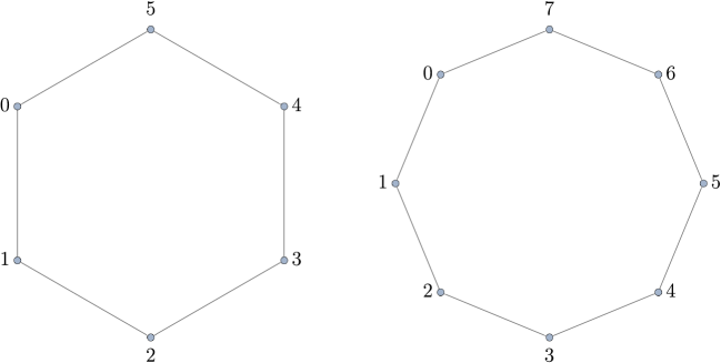
Figure 5.1: Regular pentagon and hexagon

The metric $d$ is the so called edge metric on $X_{l}$: the distance $d(k,j)$ between $k$ and $j$ is the minimal number of edges of the regular $l$-gon connecting successively $k$ and $j$. If $X_{l}\cong\mathbf{Z}/l\mathbf{Z}$ then $d(k,j)=\min\{|k-j|,l-|k-j|\}$.

For this metric if the cardinality $l=|X_{l}|=2N+1$ is odd then $N=\operatorname{diam}X_{l}$ and there are two points, namely, $N$ and $N+1$, such that $d(0,N)=d(0,N+1)=N$. If the cardinality $l=|X_{l}|=2N$ is even then $N=\operatorname{diam}X_{l}$ and there is the unique point $N$ for which $d(0,N)=N$. Moreover, we have the following distance polynomial:

$$P_{X_{l}}(q)=\left\{\begin{array}[]{ll}\vspace{3pt}q^{N}+2\sum\limits_{k=1}^{N}(1-q)^{k}q^{N-k}\,,&l=2N+1\;\mbox{is odd},\\ q^{N}+2\sum\limits_{k=1}^{N-1}(1-q)^{k}q^{N-k}+(1-q)^{N}\,,&l=2N\;\mbox{is even}\,.\end{array}\right.$$ (5.1)

It is well known that the group ${\rm Iso}(X_{l})\cong D_{l}$ where $D_{l}$ is a dihedral subgroup of order $2l$ which acts transitively on $X_{l}$. The cyclic subgroup $C_{l}<D_{l}$ acts also transitively on $X_{l}$ but the triple $(X_{l},d,D_{l})$ is symmetric in the sense of Definition 3.3 meanwhile the triple $(X_{l},d,C_{l})$ is not.

In what follows we consider only the symmetric polygonal landscapes $(X_{l},d,\Gamma,{{\boldsymbol{w}}})$, $\Gamma=D_{l}$. The stabilizer $\Gamma_{0}={\rm St}_{\Gamma}(0)\cong\mathbf{Z}/2\mathbf{Z}$. If $X_{l}\cong\{1=\varepsilon^{0},\varepsilon,\dots,\varepsilon^{l-1}\}$, then the unique non-trivial element of $\Gamma_{0}$ acts as the complex conjugation. For the model $X_{l}\cong\mathbf{Z}/l\mathbf{Z}$ it acts by the rule $k\mapsto l-k\mod l$.

There are exactly $N={\rm diam}(X_{l})$ $\Gamma_{0}$-orbits in $X$: $A_{0}=\{0\}$, $A_{k}=\{k,l-k\}$, $k=1,\dots,N-1$, and $A_{N}=\{N,N+1\}$ when $l=2N+1$ is odd, $A_{N}=\{N\}$ when $l=2N$ is even. In any case each $A_{k}=S_{k}(0)$ is the sphere of radius $k$ centered at 0.

For the orbital ring $R_{l}=R(X_{l},d,\Gamma)$ (see Section 3.3) it means that $r={\rm rk}_{\mathbf{Z}}(X_{l},d,\Gamma)=N+1$. The orbital matrices ${{\boldsymbol{M}}}_{k}={{\boldsymbol{M}}}_{A_{k}}$ have the following entries: $({{\boldsymbol{M}}}_{k})_{ab}=1$ if $d(a,b)=k$ and $({{\boldsymbol{M}}}_{k})_{ab}=0$ otherwise (for a square $X_{4}$, see Example 3.8).

The multiplication in the commutative ring $R_{l}=R(X_{l},d,D_{l})$ is slightly different for the cases of odd and even $l$. In both cases we have ${{\boldsymbol{M}}}_{0}{{\boldsymbol{M}}}_{k}={{\boldsymbol{M}}}_{k}$ since ${{\boldsymbol{M}}}_{0}={{\boldsymbol{I}}}$ is the unity of $R_{l}$.

1. Case $l=2N+1$. It can be checked that

   $${{\boldsymbol{M}}}^{2}_{k}=2{{\boldsymbol{M}}}_{0}+{{\boldsymbol{M}}}_{2k}\;\;\mbox{if}\;0<2k\leq N,\quad{{\boldsymbol{M}}}^{2}_{k}=2{{\boldsymbol{M}}}_{0}+{{\boldsymbol{M}}}_{l-2k}\;\;\mbox{if}\;N<2k\leq 2N=l-1\,.$$

   Also we have for $0<k<j\leq N$:

   $${{\boldsymbol{M}}}_{k}{{\boldsymbol{M}}}_{j}={{\boldsymbol{M}}}_{j-k}+{{\boldsymbol{M}}}_{j+k}\;\;\mbox{if}\;0<j+k\leq N,\quad{{\boldsymbol{M}}}_{k}{{\boldsymbol{M}}}_{j}={{\boldsymbol{M}}}_{j-k}+{{\boldsymbol{M}}}_{l-j-k}\;\;\mbox{if}\;N<j+k<2N=l-1\,.$$

2. Case $l=2N$. We also check that

   $${{\boldsymbol{M}}}^{2}_{k}=2{{\boldsymbol{M}}}_{0}+{{\boldsymbol{M}}}_{2k}\;\;\mbox{if}\;0<2k<N,\quad{{\boldsymbol{M}}}^{2}_{k}=2{{\boldsymbol{M}}}_{0}+{{\boldsymbol{M}}}_{l-2k}\;\;\mbox{if}\;N<2k<2N=l\,.$$

   If $2k=N$ then ${{\boldsymbol{M}}}^{2}_{k}=2{{\boldsymbol{M}}}_{0}+2{{\boldsymbol{M}}}_{N}$. If $k=N$ then ${{\boldsymbol{M}}}^{2}_{N}={{\boldsymbol{M}}}_{0}$.

Also we have for $0<k<j<N$:

$${{\boldsymbol{M}}}_{k}{{\boldsymbol{M}}}_{j}={{\boldsymbol{M}}}_{j-k}+{{\boldsymbol{M}}}_{j+k}\;\;\mbox{if}\;0<j+k<N,\quad{{\boldsymbol{M}}}_{k}{{\boldsymbol{M}}}_{j}={{\boldsymbol{M}}}_{j-k}+{{\boldsymbol{M}}}_{l-j-k}\;\;\mbox{if}\;N<j+k<2N=l\,.$$

If $k+j=N$ we have ${{\boldsymbol{M}}}_{k}{{\boldsymbol{M}}}_{j}={{\boldsymbol{M}}}_{j-k}+2{{\boldsymbol{M}}}_{N}$. If $j=N$ then ${{\boldsymbol{M}}}_{k}{{\boldsymbol{M}}}_{N}={{\boldsymbol{M}}}_{N-k}$.

Remark 5.1.

It follows that the $\mathbf{Z}$-linear mapping $\rho\colon R_{l}\longrightarrow\mathbf{Z}[2\cos(2\pi/l)]$ such that $\rho({{\boldsymbol{M}}}_{0})=1$, $\rho({{\boldsymbol{M}}}_{k})=2\cos(2\pi k/l)$ ($k=1,\dots,N$ for the case $l=2N+1$ and $k=1,\dots,N-1$ for the case $l=2N$) and, if $l=2N$, $\rho({{\boldsymbol{M}}}_{N})=-1$, is, in fact, a ring homomorphism. Note also that $\mathbf{Z}[2\cos(2\pi/l)]=\mathbf{R}\cap\mathbf{Z}[\varepsilon]$ is the ring of integers of the real field $\mathbf{R}\cap\mathbf{Q}[\varepsilon]$, $Q[\varepsilon]$ being the cyclotomic field, since $2\cos(2\pi/l)=\varepsilon+\varepsilon^{-1}$.

5.1.2 Transition matrix ${{\boldsymbol{T}}}={{\boldsymbol{T}}}_{l}$ and eigenpolynomials of the matrix ${{\boldsymbol{Q}}}={{\boldsymbol{Q}}_{l}}$

Let the symmetric triple $(X_{l},d,\Gamma)$, $\Gamma=D_{l}$, be as in the previous subsection and let the columns (rows) of all matrices under consideration be indexed by $0$, …, $l-1$ modulo $l$ (since $X_{l}\cong\mathbf{Z}/l\mathbf{Z}$). Consider the square symmetric matrix of order $l$

$${{\boldsymbol{T}}}={{\boldsymbol{T}}_{l}}=(t_{ab}):=\bigl{(}\cos(2\pi ab/l)-\sin(2\pi ab/l)\bigr{)}\;,\quad a,b\in X_{l}\cong\mathbf{Z}/l\mathbf{Z}\,.$$ (5.2)

Theorem 5.2.

The matrix ${{\boldsymbol{T}}}$ satisfies the following conditions:

1. The columns ${{\boldsymbol{t}}}_{b}$ of ${{\boldsymbol{T}}}$ compose a common eigenbasis for all orbital matrices ${{\boldsymbol{M}}}_{k}$, $k=0,\dots,N$.

2. If $l=2N+1$ is odd then

$${{\boldsymbol{T}}}^{-1}{{\boldsymbol{M}}}_{k}{{\boldsymbol{T}}}=2\operatorname{diag}(1,\cos(2\pi k/l),\cos(4\pi k/l),\dots,\cos(2\pi(l-1)k/l)),\quad k=1,\dots,N\,.$$

If $l=2N$ is even then

$${{\boldsymbol{T}}}^{-1}{{\boldsymbol{M}}}_{k}{{\boldsymbol{T}}}=2\operatorname{diag}(1,\cos(2\pi k/l),\cos(4\pi k/l),\dots,\cos(2\pi(l-1)k/l)),\quad k=1,\dots,N-1\,,$$

$${{\boldsymbol{T}}}^{-1}{{\boldsymbol{M}}}_{N}{{\boldsymbol{T}}}=\operatorname{diag}(1,-1,1,-1,\dots,1,-1)\,.$$

3. ${{\boldsymbol{T}}}^{-1}{{\boldsymbol{Q}}}{{\boldsymbol{T}}}=\operatorname{diag}(P_{0}(q),P_{1}(q),\dots,P_{l-1}(q))$ where $P_{0}(q)=P_{X_{l}}(q)$ is the distance polynomial (5.1).

If $l=2N+1$ is odd then

$$p_{j}(q)=p_{l-j}(q)=q^{N}+\sum_{k=1}^{N}2\cos(2\pi kj/l)\,(1-q)^{k}q^{N-k}\;,\quad j=1,\dots,N\;.$$ (5.3)

If $l=2N$ is even then

$$p_{j}(q)=p_{l-j}(q)=q^{N}+\sum_{k=1}^{N-1}2\cos(2\pi kj/l)\,(1-q)^{k}q^{N-k}+(-1)^{j}(1-q)^{N}\;,\quad j=1,\dots,N\;.$$ (5.4)

4. ${{\boldsymbol{T}}}^{2}=l\,{{\boldsymbol{I}}}$. In other words, ${{\boldsymbol{T}}}^{-1}=\frac{1}{l}{{\boldsymbol{T}}}$.

Proof.

1 and 2. Consider cyclic matrices ${{\boldsymbol{C}}}_{k}$ with only $l$ non-trivial entries $({{\boldsymbol{C}}}_{k})_{a,a+k}=1$ where subindices are taken modulo $l$. Note that ${{\boldsymbol{C}}}_{0}={{\boldsymbol{M}}}_{0}={{\boldsymbol{I}}}$ in any case and ${{\boldsymbol{C}}}_{N}={{\boldsymbol{M}}}_{N}$ if $l=2N$ is even. In the other cases ${{\boldsymbol{C}}}_{k}+{{\boldsymbol{C}}}_{l-k}={{\boldsymbol{M}}}_{k}$.

Consider also the vectors ${{\boldsymbol{v}}}_{j}=(1,\varepsilon^{j},\varepsilon^{2j},\dots,\varepsilon^{(l-1)j})^{T}$, $j\in X_{l}$, $\varepsilon=e^{2\pi\mathrm{i}/l}$. Straightforward checking yields

$${{\boldsymbol{C}}}_{k}{{\boldsymbol{v}}}_{j}=\varepsilon^{kj}{{\boldsymbol{v}}}_{j}\;.$$

Note that the Vandermonde determinant $\det(\varepsilon^{kj})\neq 0$. It follows that

$${{\boldsymbol{C}}}_{k}{{\boldsymbol{v}}}_{j}=\varepsilon^{kj}{{\boldsymbol{v}}}_{j}\;,\quad{{\boldsymbol{C}}}_{l-k}{{\boldsymbol{v}}}_{j}=\varepsilon^{-kj}{{\boldsymbol{v}}}_{j}\;,\quad{{\boldsymbol{C}}}_{k}{{\boldsymbol{v}}}_{l-j}=\varepsilon^{-kj}{{\boldsymbol{v}}}_{l-j}\;,\quad{{\boldsymbol{C}}}_{l-k}{{\boldsymbol{v}}}_{l-j}=\varepsilon^{kj}{{\boldsymbol{v}}}_{l-j}\,$$

since $\varepsilon^{l}=1$. If $l=2N+1$ is odd then the real vector-columns ${{\boldsymbol{t}}}_{0}={{\boldsymbol{v}}}_{0}$, ${{\boldsymbol{t}}}_{j}={\rm Re}\,{{\boldsymbol{v}}}_{j}-{\rm Im}\,{{\boldsymbol{v}}}_{l-j}$, ${{\boldsymbol{t}}}_{l-j}={\rm Re}\,{{\boldsymbol{v}}}_{l-j}+{\rm Im}\,{{\boldsymbol{v}}}_{j}$ are linearly independent eigenvectors of each ${{\boldsymbol{M}}}_{k}$ such that

$${{\boldsymbol{M}}}_{0}{{\boldsymbol{t}}}_{j}={{\boldsymbol{t}}}_{j}\,,\quad{{\boldsymbol{M}}}_{k}{{\boldsymbol{t}}}_{j}=(\varepsilon^{kj}+\varepsilon^{-kj}){{\boldsymbol{t}}}_{j}=2\cos(2\pi kj/l){{\boldsymbol{t}}}_{j},\quad k=1,\dots,N\,.$$

If $l=2N$ is even then the vector-columns ${{\boldsymbol{t}}}_{0}={{\boldsymbol{v}}}_{0}$ , ${{\boldsymbol{t}}}_{N}=(1,-1,1,-1,\dots,1,-1)^{\top}$, ${{\boldsymbol{t}}}_{j}={\rm Re}\,{{\boldsymbol{v}}}_{j}-{\rm Im}\,{{\boldsymbol{v}}}_{l-j}$, ${{\boldsymbol{t}}}_{l-j}={\rm Re}\,{{\boldsymbol{v}}}_{l-j}+{\rm Im}\,{{\boldsymbol{v}}}_{j}$ are linearly independent eigenvectors of each ${{\boldsymbol{M}}}_{k}$ such that

$${{\boldsymbol{M}}}_{0}{{\boldsymbol{t}}}_{j}={{\boldsymbol{t}}}_{j}\,,\quad{{\boldsymbol{M}}}_{k}{{\boldsymbol{t}}}_{j}=\varepsilon^{kj}+\varepsilon^{-kj}{{\boldsymbol{t}}}_{j}=2\cos(2\pi kj/l){{\boldsymbol{t}}}_{j},\quad k=1,\dots,N-1\,,\quad{{\boldsymbol{M}}}_{N}{{\boldsymbol{t}}}_{j}=\cos(\pi j){{\boldsymbol{t}}}_{j}\,.$$

In any case the transition matrix ${{\boldsymbol{T}}}$ has the form (5.2). This finishes the proof of the assertions 1 and 2.

3. Recall (3.7) that ${{\boldsymbol{Q}}}=\sum_{k=0}^{N}(1-q)^{k}q^{N-k}{{\boldsymbol{M}}}_{k}\,$. In view of the assertion 2

$${{\boldsymbol{T}}}^{-1}{{\boldsymbol{Q}}}{{\boldsymbol{T}}}=\sum_{k=0}^{N}(1-q)^{k}q^{N-k}{{\boldsymbol{T}}}^{-1}{{\boldsymbol{M}}}_{k}{{\boldsymbol{T}}}=\operatorname{diag}(p_{0}(q),p_{1}(q),\dots,p_{l-1}(q))\,.$$

Comparing the diagonal entries we get the desired result.

4. Straightforward calculations with trigonometric sums. The theorem is proved. ∎

Remark 5.3.

Note that Conjecture 3.12 is true for the triple $(X_{l},d,\Gamma)$.

5.1.3 On single peaked and alternating $G$-invariant polygonal landscapes

It is known that the subgroups of the dihedral group $D_{l}$ are, up to isomorphism, the following groups: dihedral groups $D_{m}$ and cyclic groups $C_{m}$ for $m$ dividing $l$. Note that $D_{1}\cong\mathbf{Z}/2\mathbf{Z}$.

In this section the explicit expression of the equation (4.21) is given for two-valued fitness landscapes $(X_{l},d,\Gamma=D_{l},{{\boldsymbol{w}}})$. Specifically, we consider

1. Single peaked landscapes when $X=A_{0}\sqcup A_{1}$ and $A_{1}$ consists of a single point, say, $A_{1}=\{0\}$. Thus, ${{\boldsymbol{w}}}(0)=w+s$, ${{\boldsymbol{w}}}(x)=w$, $x\neq 0$. This landscape is $G$-invariant for $G=\{1\}$.

2. Alternating landscapes for $l$-gons with even $l=2N$ (see Fig. 5.2). For these landscapes $X=A_{0}\sqcup A_{1}$ where $A_{1}=\{0,2,4,\dots,l-2\}$ and ${{\boldsymbol{w}}}(A_{0})=w$, ${{\boldsymbol{w}}}(A_{1})=w+s$. This landscape is $G$-invariant for the cyclic group $G=C_{N}$.

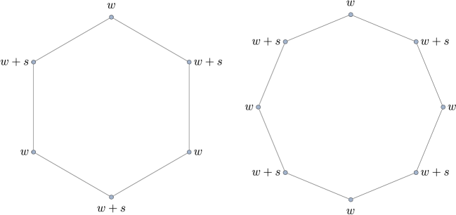
Figure 5.2: Alternating hexagonal and octagonal landscapes

1. In the case of a single peaked landscape the equation (4.21) reads

$$\frac{1}{\overline{w}-w}+\sum_{c=1}^{N-1}\frac{2P_{c}(q)}{\overline{w}P_{X}(q)-wP_{c}(q)}+\frac{HP_{N}(q)}{\overline{w}P_{X}(q)-wP_{N}(q)}=\frac{l}{s}\,,\qquad P_{0}(q)=P_{X}(q)\,,$$ (5.5)

where $H=2$ if $l=2N+1$ and $H=1$ if $l=2N$. The polynomials $P_{c}(q)$ are defined in (5.1), (5.3), (5.4).

Indeed, we need to calculate the numbers $G^{c}_{11}$ with the help of (4.16). But $a=0$, $A_{1}=\{0\}$ and in view of Theorem 5.2 $t_{0x}=lt^{(-1)}_{x0}=1$ for the transition matrix ${{\boldsymbol{T}}}$. Hence the result.

      

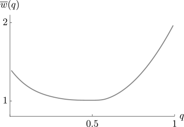
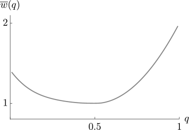
Figure 5.3: The leading eigenvalue of spectral problem (3.2) on regular $2N$-gon for single peaked landscape $w=1,s=1$. On the left $N=50$, on the right $N=200$.

In Fig. 5.3 we present two numerical examples for the considered situation. Note the absence of non-analytical behavior of $\overline{w}$, i.e., the absence of the error threshold (or phase transition).

2. In the case of an alternating landscape with $l=2N$ the straightforward calculation yields $G^{0}_{11}=G^{N}_{11}=1/2$, $G^{k}_{11}=0$ for $0<k<N$. Then the equation (4.21) is quadratic:

$$\frac{1}{\overline{w}-w}+\frac{P_{N}(q)}{\overline{w}P_{X}(q)-wP_{N}(q)}=\frac{2}{s}\,,\qquad P_{0}(q)=P_{X}(q)\,,$$

or, for $u=w/s$, $\overline{u}=\overline{w}/s$,

$$\frac{1}{\overline{u}-u}+\frac{P_{N}(q)}{\overline{u}P_{0}(q)-uP_{N}(q)}=2\,.$$ (5.6)

The polynomials $P_{0}(q),\,P_{N}(q)\in\mathbf{Z}[q]$:

$$P_{0}(q)=q^{N}+2\sum\limits_{k=1}^{N-1}(1-q)^{k}q^{N-k}+(1-q)^{N}\,,\quad P_{N}(q)=q^{N}+2\sum\limits_{k=1}^{N-1}(-1)^{k}(1-q)^{k}q^{N-k}+(-1)^{N}(1-q)^{N}\,.$$

The solution of (5.6) is (the positive square root is taken)

$$\overline{u}(q)=\frac{(2u+1)(P_{0}(q)+P_{N}(q))+\sqrt{(2u+1)^{2}(P_{0}(q)+P_{N}(q))^{2}-16u(u+1)P_{0}(q)P_{N}(q)}}{4P_{0}(q)}\,,$$ (5.7)

numerical examples are given in Fig. 5.4.

      

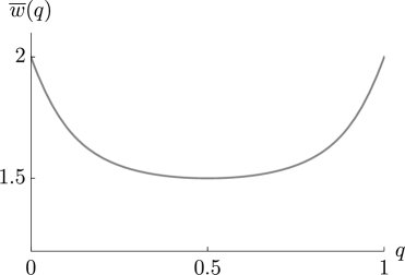
Figure 5.4: The leading eigenvalue of spectral problem (3.2) on regular $2N$-gon for alternating fitness ladscape landscape $w=1,s=1$. On the left $N=50$, on the right $N=200$.

5.2 Hyperoctahedral or dual Eigen’s landscapes

5.2.1 Preliminaries

Let $X_{n}=\{x_{0},\dots,x_{k},\dots,x_{2n-1-k},\dots,x_{2n-1}\}$ be the 0-skeleton of a regular $n$-dimensional hyperoctahedron which is the convex hull of the vertices (in $\mathbf{R}^{n}=\{(\xi_{1},\dots,\xi_{n})\}$)

$$x_{0}=(1,0,\dots,0),\,x_{2n-1}=(-1,0,\dots,0),\;\dots,$$

$$x_{k}=(0,\dots,0,1,0,\dots,0)\;(\mbox{1 stands on $(k+1)$-th position}),\quad x_{2n-1-k}=(0,\dots,0,-1,0,\dots,0),\;\dots\;.$$

A classical octahedron ($n=3$) is represented in Figure 5.5.

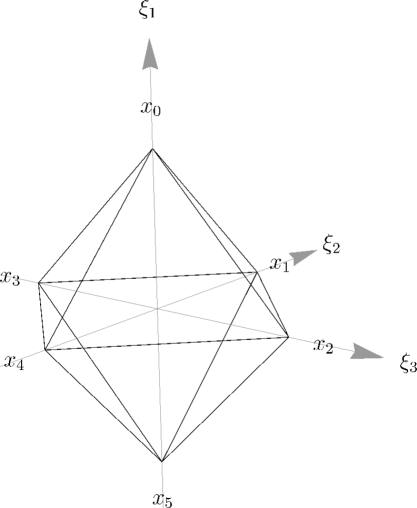
Figure 5.5: Regular octahedron.

The metric $d$ is again the edge metric metric on $X_{n}$: the distance $d(x_{k},x_{j})$ is defined as follows

$$d(x_{k},x_{j})=\left\{\begin{array}[]{l}0,\;\mbox{if}\quad k=j,\\ 2,\;\mbox{if}\quad k+j=2n-1,\\ 1,\;\mbox{otherwise}\,.\end{array}\right.$$

We have the cardinality $l=|X_{n}|=2n$ and ${\rm diam}(X_{n})=N=2$. The distance polynomial is $P_{X_{n}}(q)=q^{2}+(2n-2)(1-q)q+(1-q)^{2}$.

Since a hyperoctahedron is the dual polytope to the hypercube appearing in the classical Eigen’s model, the isometry group $\Gamma=\Gamma_{n}={\rm Iso}(X_{n})$ is a hyperoctahedral group. $\Gamma_{n}$ is isomorphic as an abstract group to the Weyl group of the root system of type $B_{n}$ or $C_{n}$ and $|\Gamma_{n}|=2^{n}\cdot n!$.

Note that the triple $(X_{n},d,\Gamma_{n})$ is symmetric in the sense of definition 3.3 and that the stabilizer $\Gamma_{0}={\rm St}_{\Gamma_{n}}(x_{0})\cong{\rm Iso}(X_{n-1})$. Indeed, viewing $x_{0}$ and $x_{2n-1}$ as the ”north” and ”south” poles respectively, we have an isometry action of $\Gamma_{0}={\rm St}_{\Gamma}(x_{0})$ on the ”equatorial” hyperoctahedron $X_{n-1}$ which is 1-sphere of $x_{0}$ with respect to the metric $d$. Then it is not hard to see that $\Gamma_{0}={\rm St}_{\Gamma_{n}}(x_{0})$ is the group of all isometries of $X_{n-1}$.

If $n\geq 2$ then there are exactly $3={\rm diam}(X_{n})+1$ $\Gamma_{0}$-orbits in $X_{n}$: namely, $A_{0}=\{x_{0}\}$, $A_{1}=\{x_{1},\dots,x_{2n-2}\}\cong X_{n-1}$, and $A_{2}=\{x_{2n-1}\}$.

For the orbital ring $R_{n}=R(X_{n},d,\Gamma)$ (see Section 3.3) it means that $r={\rm rk}_{\mathbf{Z}}(X_{l},d,\Gamma)=3$. The orbital matrices ${{\boldsymbol{M}}}_{k}={{\boldsymbol{M}}}_{A_{k}}$ have the following entries: $({{\boldsymbol{M}}}_{k})_{ab}=1$ if $d(a,b)=k$ and $({{\boldsymbol{M}}}_{k})_{ab}=0$ otherwise. For a 2-octahedron (a square) $X_{2}$ see Example 3.8, for a 3-octahedron $X_{3}$ (a classical one)

$${{\boldsymbol{M}}_{0}}={{\boldsymbol{I}}}=\left[\begin{array}[]{cccccc}1&0&0&0&0&0\\ 0&1&0&0&0&0\\ 0&0&1&0&0&0\\ 0&0&0&1&0&0\\ 0&0&0&0&1&0\\ 0&0&0&0&0&1\\ \end{array}\right],\,{{\boldsymbol{M}}_{1}}=\left[\begin{array}[]{cccccc}0&1&1&1&1&0\\ 1&0&1&1&0&1\\ 1&1&0&0&1&1\\ 1&1&0&0&1&1\\ 1&0&1&1&0&1\\ 0&1&1&1&1&0\\ \end{array}\right],\,{{\boldsymbol{M}}_{2}}=\left[\begin{array}[]{cccccc}0&0&0&0&0&1\\ 0&0&0&0&1&0\\ 0&0&0&1&0&0\\ 0&0&1&0&0&0\\ 0&1&0&0&0&0\\ 1&0&0&0&0&0\end{array}\right].$$

The multiplication table of these matrices in $R_{n}=R(X_{n},d,\Gamma_{n})$ is as follows ($n\geq 2$):

$$\begin{array}[]{|c||c|c|c|}\hline\cr\times&{{\boldsymbol{I}}}&{{\boldsymbol{M}}_{1}}&{{\boldsymbol{M}}_{2}}\\ \hline\cr{{\boldsymbol{I}}}&{{\boldsymbol{I}}}&{{\boldsymbol{M}}_{1}}&{{\boldsymbol{M}}_{2}}\\ \hline\cr{{\boldsymbol{M}}_{1}}&{{\boldsymbol{M}}_{1}}&(2n-2)({{\boldsymbol{I}}}+{{\boldsymbol{M}}_{2}})+(2n-4){{\boldsymbol{M}}_{1}}&{{\boldsymbol{M}}_{1}}\\ \hline\cr{{\boldsymbol{M}}_{2}}&{{\boldsymbol{M}}_{2}}&{{\boldsymbol{M}}_{1}}&{{\boldsymbol{I}}}\\ \hline\cr\end{array}$$

5.2.2 Transition matrix ${{\boldsymbol{T}}}={{\boldsymbol{T}}}_{n}$ and eigenpolynomials of the matrix ${{\boldsymbol{Q}}}={{\boldsymbol{Q}}_{n}}$

Let the symmetric triple $(X_{n},d,\Gamma_{n})$ be as in the previous subsection and let the columns (rows) of all matrices under consideration be indexed by $0$, …, $2n-1$ corresponding to $x_{0},\dots,x_{2n-1}$. Consider the following four matrices of order $n$ ($n\geq 2$):

$${{\boldsymbol{T}}_{00}}=\left[\begin{array}[]{crrcr}1&1&1&\dots&1\\ 1&-1&0&\dots&0\\ 1&0&-1&\dots&0\\ \vdots&\vdots&\vdots&\ddots&\vdots\\ 1&0&0&\cdots&-1\\ \end{array}\right],\;{{\boldsymbol{T}}_{01}}=\left[\begin{array}[]{rlrrr}1&\dots&1&1&1\\ 0&\dots&0&-1&1\\ 0&\dots&-1&0&1\\ \vdots&.^{\,\displaystyle{.^{\,.}}}&\vdots&\vdots&\vdots\\ -1&\cdots&0&0&1\\ \end{array}\right],$$

$${{\boldsymbol{T}}_{10}}=\left[\begin{array}[]{crrcr}1&0&0&\cdots&-1\\ \vdots&\vdots&\vdots&.^{\,\displaystyle{.^{\,.}}}&\vdots\\ 1&0&-1&\dots&0\\ 1&-1&0&\dots&0\\ 1&1&1&\dots&1\\ \end{array}\right],\;{{\boldsymbol{T}}_{11}}=\left[\begin{array}[]{rrrrr}1&\cdots&0&0&-1\\ \vdots&\ddots&\vdots&\vdots&\vdots\\ 0&\dots&1&0&-1\\ 0&\dots&0&1&-1\\ -1&\dots&-1&-1&-1\\ \end{array}\right].$$

Here the entries of the first row and column of the matrix ${{\boldsymbol{T}}_{00}}$ are equal to 1, the diagonal entries, except for the first one, are equal to $-1$, and the other entries are trivial. The matrices ${{\boldsymbol{T}}_{01}}$ and ${{\boldsymbol{T}}_{10}}$ are the horizontal and vertical mirror copies of ${{\boldsymbol{T}}_{00}}$, the matrix ${{\boldsymbol{T}}_{11}}$ is the horizontal mirror copy of ${{\boldsymbol{T}}_{10}}$ multiplied by $-1$.

Consider the square symmetric matrix of order $2n$

$${{\boldsymbol{T}}}={{\boldsymbol{T}}_{n}}=\left[\begin{array}[]{cc}{{\boldsymbol{T}}_{00}}&{{\boldsymbol{T}}_{01}}\\ {{\boldsymbol{T}}_{10}}&{{\boldsymbol{T}}_{11}}\\ \end{array}\right]\,.$$ (5.8)

We also introduce the following four matrices of order $n$:

$${{\boldsymbol{K}}_{00}}=\left[\begin{array}[]{crrcr}1&1&1&\dots&1\\ 1&1-n&1&\dots&1\\ 1&1&1-n&\dots&1\\ \vdots&\vdots&\vdots&\ddots&\vdots\\ 1&1&1&\cdots&1-n\\ \end{array}\right],\;{{\boldsymbol{K}}_{01}}=\left[\begin{array}[]{rlrrr}1&\dots&1&1&1\\ 1&\dots&1&1-n&1\\ 1&\dots&1-n&1&1\\ \vdots&.^{\,\displaystyle{.^{\,.}}}&\vdots&\vdots&\vdots\\ 1-n&\cdots&1&1&1\\ \end{array}\right],$$

$${{\boldsymbol{K}}_{10}}=\left[\begin{array}[]{crrcr}1&1&1&\cdots&1-n\\ \vdots&\vdots&\vdots&.^{\,\displaystyle{.^{\,.}}}&\vdots\\ 1&1&1-n&\dots&1\\ 1&1-n&1&\dots&1\\ 1&1&1&\dots&1\\ \end{array}\right],\;{{\boldsymbol{K}}_{11}}=\left[\begin{array}[]{rrrrr}n-1&\cdots&-1&-1&-1\\ \vdots&\ddots&\vdots&\vdots&\vdots\\ -1&\dots&n-1&-1&-1\\ -1&\dots&-1&n-1&-1\\ -1&\dots&-1&-1&-1\\ \end{array}\right].$$

Here the diagonal entries of the matrix ${{\boldsymbol{K}}_{00}}$, except for $k_{00}=1$, are equal to $1-n$, and the other entries are equal to 1. The matrices ${{\boldsymbol{K}}_{01}}$ and ${{\boldsymbol{K}}_{10}}$ are the horizontal and vertical mirror copies of ${{\boldsymbol{K}}_{00}}$, the matrix ${{\boldsymbol{K}}_{11}}$ is the horizontal mirror copy of ${{\boldsymbol{K}}_{10}}$ multiplied by $-1$.

Consider the square symmetric matrix of order $2n$

$${{\boldsymbol{K}}}={{\boldsymbol{K}}_{n}}=\left[\begin{array}[]{cc}{{\boldsymbol{K}}_{00}}&{{\boldsymbol{K}}_{01}}\\ {{\boldsymbol{K}}_{10}}&{{\boldsymbol{K}}_{11}}\\ \end{array}\right]\,.$$ (5.9)

Theorem 5.4.

The matrix ${{\boldsymbol{T}}}={{\boldsymbol{T}}}_{n}$, $n\geq 2$, satisfies the following conditions:

1. $\det({{\boldsymbol{T}}}_{n})=(-1)^{n}\cdot 2^{n}\cdot n^{2}$, consequently, ${{\boldsymbol{T}}}_{n}$ is a non-degenerate matrix.

2. ${{\boldsymbol{T}}}^{-1}_{n}=\frac{1}{2n}{{\boldsymbol{K}}}_{n}$.

3. The columns ${{\boldsymbol{t}}}_{b}$ ($b=0,\dots,2n-1$) of ${{\boldsymbol{T}}}$ compose a common eigenbasis for each orbital matrix ${{\boldsymbol{M}}}_{0}$, ${{\boldsymbol{M}}}_{1}$, ${{\boldsymbol{M}}}_{2}$.

4. More precisely,

$${{\boldsymbol{T}}}^{-1}{{\boldsymbol{M}}}_{1}{{\boldsymbol{T}}}=\operatorname{diag}(2n-2,\underbrace{-2,\dots,-2}_{n-1\;\mbox{\scriptsize{times}}},\underbrace{0,\dots,0}_{n\;\mbox{\scriptsize{times}}})\,,$$

$${{\boldsymbol{T}}}^{-1}{{\boldsymbol{M}}}_{2}{{\boldsymbol{T}}}=\operatorname{diag}(\underbrace{1,\dots,1}_{n\;\mbox{\scriptsize{times}}},\underbrace{-1,\dots,-1}_{n\;\mbox{\scriptsize{times}}})\,.$$

5. Let ${{\boldsymbol{Q}}}={{\boldsymbol{Q}}}_{n}=\left((1-q)^{d(x_{a},x_{b})}\cdot q^{2-d(x_{a},x_{b})}\right)$. Then

$${{\boldsymbol{T}}}^{-1}{{\boldsymbol{Q}}}{{\boldsymbol{T}}}=\operatorname{diag}(P_{0}(q),P_{1}(q),\dots,P_{2n-1}(q))=$$

$$=\operatorname{diag}(q^{2}+(2n-2)(1-q)q+(1-q)^{2},\underbrace{(2q-1)^{2},\dots,(2q-1)^{2}}_{n-1\;\mbox{\scriptsize{times}}},\underbrace{2q-1,\dots,2q-1}_{n\;\mbox{\scriptsize{times}}})\,.$$

Proof.

1. Subtracting the row 0 from the row $2n-1$, the row 1 from the row $2n-2$, …, the row $n-1$ from the row $n$ (note that the subindices of matrix entries range from $0$ to $2n-1$) we get

$$\det({{\boldsymbol{T}}})=\det\left[\begin{array}[]{cc}{{\boldsymbol{T}}_{00}}&{{\boldsymbol{T}}_{01}}\\ {{\boldsymbol{T}}_{10}}&{{\boldsymbol{T}}_{11}}\\ \end{array}\right]=\det\left[\begin{array}[]{cc}{{\boldsymbol{T}}_{00}}&{{\boldsymbol{T}}_{01}}\\ {{\boldsymbol{0}}}&{{\boldsymbol{2}}T_{11}}\\ \end{array}\right]=2^{n}\det({{\boldsymbol{T}}_{00}})\det({{\boldsymbol{T}}_{11}}).$$

Adding the sum of columns 2, …, $n$ to the first column of the matrix ${{\boldsymbol{T}}_{00}}$ we obtain the equality $\det({{\boldsymbol{T}}_{00}})=(-1)^{n-1}n$. In a similar way we obtain that $\det({{\boldsymbol{T}}_{11}})=-n$. Hence the desired result.

2. Straightforward checking shows that ${{\boldsymbol{T}}}_{n}{{\boldsymbol{K}}_{n}}=2n{{\boldsymbol{I}}}$. Note that the matrix ${{\boldsymbol{T}}_{00}}$ appears as a transition matrix for a simplicial landscape, see [25, Section 6] for the inverse ${{\boldsymbol{T}}^{-1}_{00}}$ and for more details.

3 and 4. Straightforward calculations show that

$${{\boldsymbol{M}}_{1}}{{\boldsymbol{t}}}_{0}=(2n-2){{\boldsymbol{t}}}_{0},\quad{{\boldsymbol{M}}_{1}}{{\boldsymbol{t}}}_{b}=-2{{\boldsymbol{t}}}_{b}\;\;(b=1,\dots,n-1),\quad{{\boldsymbol{M}}_{1}}{{\boldsymbol{t}}}_{b}={{\boldsymbol{0}}}\;\;(b=n,\dots,2n-1)\,,$$

$${{\boldsymbol{M}}_{2}}{{\boldsymbol{t}}}_{b}={{\boldsymbol{t}}}_{b}\;\;(b=0,\dots,n-1),\quad{{\boldsymbol{M}}_{1}}{{\boldsymbol{t}}}_{b}=-{{\boldsymbol{t}}}_{b}\;\;(b=n,\dots,2n-1)\,.$$

5. Since ${{\boldsymbol{Q}}}=q^{2}{{\boldsymbol{I}}}+q(1-q){{\boldsymbol{M}}}_{1}+(1-q)^{2}{{\boldsymbol{M}}}_{2}$ and in view of 3 we get

$${{\boldsymbol{T}}}^{-1}{{\boldsymbol{Q}}}{{\boldsymbol{T}}}=q^{2}{{\boldsymbol{I}}}+q(1-q)\operatorname{diag}(2n-2,\underbrace{-2,\dots,-2}_{n-1\;\mbox{\scriptsize{times}}},\underbrace{0,\dots,0}_{n\;\mbox{\scriptsize{times}}})+(1-q)^{2}\operatorname{diag}(\underbrace{1,\dots,1}_{n\;\mbox{\scriptsize{times}}},\underbrace{-1,\dots,-1}_{n\;\mbox{\scriptsize{times}}})=$$

$$=\operatorname{diag}(q^{2}+(2n-2)(1-q)q+(1-q)^{2},\underbrace{(2q-1)^{2},\dots,(2q-1)^{2}}_{n-1\;\mbox{\scriptsize{times}}},\underbrace{2q-1,\dots,2q-1}_{n\;\mbox{\scriptsize{times}}})\,.$$

The theorem is proved. ∎

Remark 5.5.

Note that Conjecture 3.12 is true for the triple $(X_{n},d,\Gamma_{n})$.

5.2.3 On single peaked $G$-invariant hyperoctahedral landscapes

In this subsection the explicit expression of the equation (4.21) is given for 2-fitness hyperoctahedral landscapes $(X_{n},d,\Gamma_{n},{{\boldsymbol{w}}})$.

Consider a single peaked landscape for which $X_{n}=A_{0}\sqcup A_{1}$ and $A_{1}$ consists of a single point, say, $A_{1}=\{x_{0}\}$. Thus, ${{\boldsymbol{w}}}(x_{0})=w+s$, ${{\boldsymbol{w}}}(x_{k})=w$, $k=1,\dots,2n-1$. This landscape is $G$-invariant under the action of the trivial group $G=\{1\}$.

In the case of a single peaked landscape the equation (4.21) reads

$$\frac{G_{11}^{0}}{\overline{w}-w}+\frac{G_{11}^{1}(2q-1)^{2}}{\overline{w}P_{X}(q)-w(2q-1)^{2}}+\frac{G_{11}^{2}(2q-1)}{\overline{w}P_{X}(q)-w(2q-1)}=\frac{l}{s}\,,$$ (5.10)

where $P_{X}(q)=p_{0}(q)=q^{2}+(2n-2)q(1-q)+(1-q)^{2}$ is the distance polynomial and, in view of the assertion 2 of Theorem 5.4 and (4.16),

$$G_{11}^{0}=\frac{1}{2n}\,\quad G_{11}^{1}=\frac{n-1}{2n},\quad G_{11}^{2}=\frac{n}{2n}=\frac{1}{2}\,.$$

Finally, for the parameters $u=w/s$, $\overline{u}=\overline{w}/s$ we obtain the (cubic) equation

$$\frac{1}{\overline{u}-u}+\frac{(n-1)(2q-1)^{2}}{\overline{u}P_{X}(q)-u(2q-1)^{2}}+\frac{n(2q-1)}{\overline{u}P_{X}(q)-u(2q-1)}=2n\,.$$ (5.11)

Numerical illustrations are given in Fig. 5.6. Note that in this case, different from the polygonal landscapes we considered in Section 5.1, the numerical experiments indicate that this model possesses the error threshold.

      

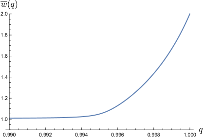
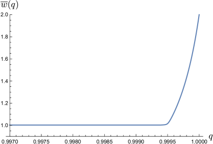
Figure 5.6: The leading eigenvalue of spectral problem (3.2) on hyperoctahedral landscape for SPL $w=1,s=1$. On the left $n=100$, on the right $n=1000$.

6 Concluding remarks

The main contribution of the present paper is twofold. First, we introduced a generalized algebraic quasispecies model in which the standard binary hypercube of Eigen’s model is replaced with an arbitrary finite metric space $X$. Second, we showed that if the structure of the fitness landscape is related to the isometry group of $X$ then a progress can be made in analytical investigation of the corresponding spectral problem. In particular, we found an explicit form of the algebraic equation for the leading eigenvalue (equation (4.20)).

At the same time, there are a number of open questions, which would be interesting to work on using the framework we suggest.

While the equation for $\overline{w}$ is written in the general form, in all the examples we considered here and in [25] we deal with the simplest case of two-valued fitness landscapes, when $X=A_{0}\bigsqcup A_{1}$. It is important to consider examples with more complicated partition of $X$. For example, the so-called mesa landscapes [31] have exactly this form.

The error threshold phenomenon (see Fig. 2.2) was not analyzed in the present text. We remark that the error threshold was proven to exist for a simplicial mutation landscape in [25]. It looks plausible to conjecture that for the considered in the present text $m$-gon landscapes the error threshold is absent whereas for the hyperoctahedral mutation landscape it does exist. In general, we now have a more general question to ask: What are the properties of a finite metric space $X$ that guarantee the existence of the error threshold at least for some fitness landscapes ${\boldsymbol{w}}$?

Finally, more detailed analysis of the connections of the considered spectral problems with the Ising model is necessary. The proof that 2D Ising model possesses the phase transition, given by Onsager, is very non-elementary. On the other hand, for the simplicial and hyperoctahedral mutation landscapes the algebraic equation for the leading eigenvalue has degree 2 and 3 respectively and they provide much simpler examples of modeling systems that possess phase transition behavior.

Appendix A Resulting tables

In the following Table 1 several known homogeneous symmetric triples $(X,d,\Gamma)$ of the landscapes are presented. Here $H_{n}$ is a hyperoctahedral group (the Weyl group of root system $B_{n}$ or $C_{n}$ ) of order $2^{n}n!$, $S_{n}$ is a symmetric group, $D_{n}$ is a dihedral group of order $2n$, $A_{5}$ is the alternating group of order 60, $D_{1}\cong\mathbf{Z}/2\mathbf{Z}$, $\Gamma_{0}={\rm St}(x)$, $x\in X$. For regular polytopes $P$ the metric space $(X,d)$ consists of the set $X=P^{(0)}$ of vertices, the metric $d$ is the edge metric (see Example 3.1).

$$\begin{array}[]{|l|c|c|c|c|c|c|c|}\hline\cr\;\mbox{Landscape}&X&d&l=|X|&\operatorname{diam}X&\Gamma&\Gamma_{0}&r={\rm rk}_{\mathbf{Z}}R(X,d,\Gamma)\\ \hline\cr\phantom{\rule{0.0pt}{12.0pt}}1.\;\mbox{\it Hypercubic,}&\{0,1\}^{n}&Hamming&2^{n}&n&H_{n}&S_{n}&n+1\\ \mbox{\it or Eigen's}&&(edge)&&&&&\\ &&metric&&&&&\\ \hline\cr\phantom{\rule{0.0pt}{12.0pt}}2.\;\mbox{\it Simplicial}&X_{n}&edge&n+1&1&S_{n+1}&S_{n}&2\\ &&metric&&&&&\\ \hline\cr\phantom{\rule{0.0pt}{12.0pt}}3.\;\mbox{\it Polygonal}&X_{2n}&edge&2n&n&D_{2n}&D_{1}&n+1\\ &&metric&&&&&\\ \hline\cr\phantom{\rule{0.0pt}{12.0pt}}4.\;\mbox{\it Polygonal}&X_{2n+1}&edge&2n+1&n&D_{2n+1}&D_{1}&n+1\\ &&metric&&&&&\\ \hline\cr\phantom{\rule{0.0pt}{12.0pt}}5.\,\mbox{\it Hyper-}&X_{n}&edge&2n&2&H_{n}&H_{n-1}&3\\ \mbox{\it octahedral}&&metric&&&&&\\ \hline\cr\phantom{\rule{0.0pt}{12.0pt}}6.\,\mbox{\it Dodeca-}&X=P^{(0)}&edge&20&5&A_{5}&D_{3}&6\\ \mbox{\it hedral}&&metric&&&&&\\ \hline\cr\phantom{\rule{0.0pt}{12.0pt}}7.\,\mbox{\it Icosa-}&X=P^{(0)}&edge&12&3&A_{5}&D_{5}&4\\ \mbox{\it hedral}&&metric&&&&&\\ \hline\cr\end{array}$$

Table 1: Examples of the homogeneous symmetric triples $(X,d,\Gamma)$

In Table 2 the eigenpolynomials and their multiplicities (in brackets) of the matrix ${{\boldsymbol{Q}}}$ are given. The first one is always the (leading) distance polynomial of multiplicity 1.

$$\begin{array}[]{|l|c|c|}\hline\cr\;\mbox{Landscape}&X&\mbox{Eigenpolynomials of}\;{{\boldsymbol{Q}}}\;\mbox{(their multiplicities)}\\ \hline\cr\phantom{\rule{0.0pt}{12.0pt}}1.\;\mbox{\it Hypercubic,}&X_{n}&P_{X}(q)\equiv 1\;,\;(1),\\ \mbox{\it or Eigen's}&&P_{j}(q)=(2q-1)^{j}\;,\;\left(\binom{n}{j}\right),\quad j=1,\dots,n\\ \hline\cr\phantom{\rule{0.0pt}{12.0pt}}2.\;\mbox{\it Simplicial}&X_{n}&P_{X}(q)=q+n(1-q)\;,\;(1),\\ &&P_{1}(q)=2q-1\;,\;(n)\\ \hline\cr\phantom{\rule{0.0pt}{12.0pt}}3.\;\mbox{\it Polygonal}&X_{n},&P_{X}(q)=q^{N}+2\sum\limits_{k=1}^{N-1}(1-q)^{k}q^{N-k}+(1-q)^{N}\;,\;(1),\\ &n=2N&P_{j}(q)=q^{N}+\sum\limits_{k=1}^{N-1}2\cos(2\pi kj/l)\,(1-q)^{k}q^{N-k}+(-1)^{j}(1-q)^{N}\;,\;(2),\\ &&j=1,\dots,N-1,\\ &&P_{N}(q)=q^{N}+2\sum\limits_{k=1}^{N-1}(-1)^{k}(1-q)^{k}q^{N-k}+(-1)^{N}(1-q)^{N}\;,\;(1),\\ \hline\cr\phantom{\rule{0.0pt}{12.0pt}}4.\;\mbox{\it Polygonal}&X_{n},&P_{X}(q)=q^{N}+2\sum\limits_{k=1}^{N}(1-q)^{k}q^{N-k}\;,\;(1),\\ &n=2N+1&P_{j}(q)=q^{N}+\sum\limits_{k=1}^{N}2\cos(2\pi kj/l)\,(1-q)^{k}q^{N-k}\;,\;(2),\\ &&j=1,\dots,N\\ \hline\cr\phantom{\rule{0.0pt}{12.0pt}}5.\;\mbox{\it Hyper-}&X_{n}&P_{X}(q)=q^{2}+(2n-2)(1-q)q+(1-q)^{2}\;,\;(1),\\ \mbox{\it octahedral}&&P_{1}(q)=(2q-1)^{2}\;,\;(n-1),\\ &&P_{2}(q)=2q-1\;,\;(n)\\ \hline\cr\phantom{\rule{0.0pt}{12.0pt}}6.\;\mbox{\it Dodeca-}&X&P_{X}(q)=2q^{4}-4q^{3}+4q^{2}-2q+1\;,\;(1),\\ \;\mbox{\it hedral}&&P_{1}(q)=(-2q^{4}+4q^{3}+q^{2}-3q+1)(2q-1)\;,\;(4),\\ &&P_{2}(q)=(3q^{4}-6q^{3}+6q^{2}-3q+1+\sqrt{5}(q^{4}-2q^{3}+2q^{2}-q))\times\\ &&\times(2q-1)\;,\;(3),\\ &&P_{3}(q)=(3q^{4}-6q^{3}+6q^{2}-3q+1-\sqrt{5}(q^{4}-2q^{3}+2q^{2}-q))\times\\ &&\times(2q-1)\;,\;(3),\\ &&P_{4}(q)=(3q^{2}-3q+1)(2q-1)^{2}\;\;(4),\\ &&P_{5}(q)=(2q-1)^{2}\;,\;(5)\\ \hline\cr\phantom{\rule{0.0pt}{12.0pt}}7.\;\mbox{\it Icosa-}&X&P_{X}(q)=-2q^{2}+2q+1\;,\;(1),\\ \;\mbox{\it hedral}&&P_{1}(q)=(q^{2}-q+1+\sqrt{5}(q^{2}-q))(2q-1)\;,\;(3),\\ &&P_{2}(q)=(q^{2}-q+1-\sqrt{5}(q^{2}-q))(2q-1)\;,\;(3),\\ &&P_{3}(q)=(2q-1)^{2}\;,\;(5)\\ \hline\cr\end{array}$$

Table 2: Examples of eigenpolynomials and their multiplicities for several generalized mutation matrices ${\boldsymbol{Q}}$ corresponding to particular triples $(X,d,\Gamma)$

References

- [1] E. Baake and W. Gabriel. Biological evolution through mutation, selection, and drift: An introductory review. In D. Stauffer, editor, Annual Reviews of Computational Physics VII, pages 203–264. World Scientific, 1999.
- [2] E. Baake and H.-O. Georgii. Mutation, selection, and ancestry in branching models: a variational approach. Journal of Mathematical Biology, 54(2):257–303, Feb 2007.
- [3] E. Baake and H. Wagner. Mutation–selection models solved exactly with methods of statistical mechanics. Genetical research, 78(1):93–117, 2001.
- [4] A. S. Bratus, A. S. Novozhilov, and Y. S. Semenov. Linear algebra of the permutation invariant Crow–Kimura model of prebiotic evolution. Mathematical Biosciences, 256:42–57, 2014.
- [5] K. S. Brown. Cohomology of groups, volume 87. Springer, 2012.
- [6] R. Cerf and J. Dalmau. The quasispecies distribution. arXiv preprint arXiv:1609.05738, 2016.
- [7] R. Cerf and J. Dalmau. Quasispecies on class-dependent fitness landscapes. Bulletin of mathematical biology, 78(6):1238–1258, 2016.
- [8] H. S. M. Coxeter. Regular polytopes. Courier Corporation, 1973.
- [9] P. de la Harpe. Topics in geometric group theory. University of Chicago Press, 2000.
- [10] A. W. M. Dress and D. S. Rumschitzki. Evolution on sequence space and tensor products of representation spaces. Acta Applicandae Mathematica, 11(2):103–115, 1988.
- [11] M. Eigen. Selforganization of matter and the evolution of biological macromolecules. Naturwissenschaften, 58(10):465–523, 1971.
- [12] M. Eigen, J. McCaskill, and P. Schuster. Molecular quasi-species. Journal of Physical Chemistry, 92(24):6881–6891, 1988.
- [13] W. Feit. The representation theory of finite groups, volume 2. Elsevier, 1982.
- [14] J. Hermisson, O. Redner, H. Wagner, and E. Baake. Mutation-selection balance: ancestry, load, and maximum principle. Theoretical Population Biology, 62(1):9–46, Aug 2002.
- [15] K. Jain and J. Krug. Adaptation in Simple and Complex Fitness Landscapes. In U. Bastolla, M. Porto, H. Eduardo Roman, and M. Vendruscolo, editors, Structural approaches to sequence evolution, chapter 14, pages 299–339. Springer, 2007.
- [16] A. A. Kirillov. Elements of the Theory of Representations, volume 145. Springer, 1976.
- [17] I. Leuthäusser. An exact correspondence between Eigen s evolution model and a two-dimensional Ising system. The Journal of Chemical Physics, 84(3):1884–1885, 1986.
- [18] I. Leuthäusser. Statistical mechanics of Eigen’s evolution model. Journal of statistical physics, 48(1):343–360, 1987.
- [19] L. Onsager. Crystal statistics. i. a two-dimensional model with an order-disorder transition. Physical Review, 65(3-4):117, 1944.
- [20] D. S. Rumschitzki. Spectral properties of Eigen evolution matrices. Journal of Mathematical Biology, 24(6):667–680, 1987.
- [21] D. B. Saakian and C. K. Hu. Exact solution of the Eigen model with general fitness functions and degradation rates. Proceedings of the National Academy of Sciences USA, 103(13):4935–4939, 2006.
- [22] P. Schuster. Quasispecies on fitness landscapes. In E. Domingo and P. Schuster, editors, Quasispecies: From Theory to Experimental Systems, Current Topics in Microbiology and Immunology, pages 61–120. Springer, 2015.
- [23] Y. Semenov. Rings associated with hyperbolic groups. Communications in Algebra, 22(15):6323–6347, 1994.
- [24] Y. S. Semenov and A. S. Novozhilov. Exact solutions for the selection-mutation equilibrium in the Crow-Kimura evolutionary model. Mathematical Biosciences, 266:1–9, 2015.
- [25] Y. S. Semenov and A. S. Novozhilov. On Eigen s quasispecies model, two-valued fitness landscapes, and isometry groups acting on finite metric spaces. Bulletin of mathematical biology, 78(5):991–1038, 2016.
- [26] J.-P. Serre. Linear representations of finite groups, volume 42. Springer, 2012.
- [27] J. Swetina and P. Schuster. Self-replication with errors: A model for polvnucleotide replication. Biophysical Chemistry, 16(4):329–345, 1982.
- [28] C. J. Thompson. Mathematical statistical mechanics. New York: Macmillan, 1972.
- [29] T. Wiehe. Model dependency of error thresholds: the role of fitness functions and contrasts between the finite and infinite sites models. Genetical research, 69(02):127–136, 1997.
- [30] C. O. Wilke. Quasispecies theory in the context of population genetics. BMC Evolutionary Biology, 5(1):44, 2005.
- [31] A. Wolff and J. Krug. Robustness and epistasis in mutation-selection models. Physical biology, 6(3):036007, 2009.