A-posteriori error estimation and adaptivity for nonlinear parabolic equations using IMEX-Galerkin discretization of primal and dual equations

Abstract

While many methods exist to discretize nonlinear time-dependent partial differential equations (PDEs), the rigorous estimation and adaptive control of their discretization errors remains challenging. In this paper, we present a methodology for duality-based a posteriori error estimation for nonlinear parabolic PDEs, where the full discretization of the PDE relies on the use of an implicit-explicit (IMEX) time-stepping scheme and the finite element method in space. The main result in our work is a decomposition of the error estimate that allows to separate the effects of spatial and temporal discretization error, and which can be used to drive adaptive mesh refinement and adaptive time-step selection. The decomposition hinges on a specially-tailored IMEX discretization of the dual problem. The performance of the error estimates and the proposed adaptive algorithm is demonstrated on two canonical applications: the elementary heat equation and the nonlinear Allen–Cahn phase-field model.

65M15, 65M20, 65M50

1 Introduction

Nonlinear parabolic PDEs are ubiquitous in science, however, their efficient numerical solution remains challenging. Implicit-explicit (IMEX) methods have been widely used for the time integration of complex time-dependent PDEs with terms of different type [1, 8]. Recently, a number of IMEX time-stepping schemes, paired with spatial Galerkin finite-element discretizations, have been proposed for phase-field models [35, 18, 37, 30, 34], which are currently a much-studied class of nonlinear parabolic problems [21, 24, 20, 28, 19]. When the PDE solution displays alternating fast and slow variations, the numerical discretization can, obviously, benefit significantly from adaptivity in both space and time.

This paper is devoted to the development of a posteriori error estimates and corresponding adaptive algorithms for these popular discretizations. In particular, we consider dual-based error estimates that assess the discretization error with respect to user specified quantities of interest describing the goal of the analyses. The quantities of interest might, for instance, be physical quantities or some appropriate norms of the error of the solution (e.g. energy norm, $L^{2}$ norm). To efficiently drive adaptive mesh refinement and adaptive time-step selection, the error estimates need to address the temporal and the spatial discretization errors separately.

There have been several studies on goal-oriented adaptive techniques for parabolic equations during the last decade, but mostly in the context of space-time (discontinuous) Galerkin finite element discretization, see for instance Eriksson and Johnson [13, 14, 15, 16], Schmich and Vexler [27], Carey et al. [10], Bermejo and Carpio [6], Braack et al. [9], Besier and Rannacher[7], and Asner et al. [2]. Very little progress has been made for parabolic equations discretized using IMEX time-stepping schemes.

Recently, Chaudhry et al. [11, 12] proposed a posteriori error estimates for various IMEX schemes, based on an equivalence relation between IMEX schemes and time-Galerkin finite element methods. They rewrite the time-Galerkin method using special numerical quadrature rules and carry out a standard duality-based analysis for the resultant approximations. The splitting of the temporal and the spatial error contributions in these error estimates are commonly achieved by inserting and subtracting suitable projections of the dual solution.

The objective of this paper is to present an alternative approach to duality-based a posteriori error estimates for fully discretized semi-linear parabolic PDEs using conforming finite elements in space and first-order IMEX schemes in time. Contrary to Chaudhry et al, in our approach we directly obtain a posteriori error estimates without resorting to an interpretation of IMEX as a Galerkin-in-time method. This paper is a follow-up to our recent paper [29], where we only considered errors due to spatial discretization. The focus of this work is on the total discretization error which contains both the spatial and temporal parts.

The starting point of our analysis is the exact duality-based error representation, which is a duality pairing of the global space-time residual with the solution of the mean-value-linearized (backward-in-time) dual problem. This error representation can be decomposed into various distinct residuals weighted by the same dual solution. A fundamental framework for successfully decomposing the residuals for (non)linear parabolic PDEs, discretized by a classical A-stable $\theta$-scheme in time, has been developed by Verfürth [33] in the context of energy-based a posteriori error analysis.

By extending Verfürth’s framework to IMEX schemes and a duality-based error analysis, we will decompose the error representation into three contributions which can be associated to the temporal and spatial discretization error, and additionally data oscillation. This novel decomposition hinges on a special nonstandard IMEX discretization of the dual problem. We then propose a general space-time adaptive algorithm for an efficient distribution of the discretization parameters: a set of time steps and the refined mesh at each time step.

This work is structured as follows. In Section 2, we introduce the abstract setting for a general (non)linear parabolic PDE and its IMEX-Galerkin discretization. Section 3 is devoted to the methodology for a space-time decomposition of a duality-based a posteriori error estimate. After having established computable error estimates in Section 4, we propose the associated adaptive algorithm in Section 5. The application to the elementary heat equation and the nonlinear Allen–Cahn equation (an elementary phase-field model), together with numerical results are presented in Section 6, after which we present our conclusions.

2 Abstract setting

In this section, we start by introducing an abstract setting of nonlinear parabolic PDEs and the corresponding dual problem in weak formulations. Then we present the discretization of the primal problem using IMEX time-stepping schemes and conforming finite elements in space.

2.1 Weak formulation and error representation

As a model problem we consider a general semi-linear parabolic equation in a bounded space-time domain $\Omega\times(0,T]$ with $\Omega\subset\mathbb{R}^{d}$, $d=1,2,3$, having natural boundary conditions. To provide a setting for the weak formulation, we denote by $\mathcal{V}$ a suitable Hilbert space and by $\mathcal{V}^{*}$ its dual space, such that $\mathcal{V}\subset L^{2}(\Omega)\subset\mathcal{V}^{*}$ with continuous embeddings. We denote the inner product in $L^{2}(\Omega)$ by $(\cdot,\cdot)$, and duality pairings between $\mathcal{V}^{*}$ and $\mathcal{V}$ by $\left\langle\cdot,\cdot\right\rangle$. By defining $\mathcal{W}:=\left\{v\in L^{2}(0,T;\mathcal{V}),\partial_{t}v\in L^{2}(0,T;\mathcal{V}^{*})\right\}$ as a suitable space for $u$, the weak form reads: find $u\in\mathcal{W}_{u^{0}}:=\left\{v\in\mathcal{W}:v(0)=u^{0}\right\}$ such that $\forall v\in L^{2}(0,T;\mathcal{V})$

(1) $$\int_{0}^{T}\Big{(}\langle\partial_{t}u,v\rangle+\mathcal{B}(u,v)+\mathcal{N}(u;v)\Big{)}\,\mathrm{d}t=\int_{0}^{T}\langle f,v\rangle\,\mathrm{d}t$$

where $f\in L^{2}(0,T;\mathcal{V}^{*})$, $u^{0}\in L^{2}(\Omega)$, the semi-linear form $\mathcal{N}(\cdot;\cdot)$ of a sufficiently smooth nonlinear operator represents the nonlinear components which is linear with respect to arguments on the right of the semicolon, and $\mathcal{B}(\cdot,\cdot)$ is the bilinear form of a elliptic self-adjoint operator. A prime example of the abstract setting is the Allen–Cahn equation $\partial_{t}u-\Delta u+\frac{1}{\varepsilon^{2}}\psi^{\prime}(u)=0$, which will be discussed later in Section 6.1.

Given the solution $u$, we consider the quantity

(2) $$\mathcal{Q}(u):=\left(\bar{q},u(T)\right)+\int_{0}^{T}(q,u)\,\mathrm{d}t,$$

with $\bar{q}\in L^{2}(\Omega)$ and $q\in L^{2}(0,T;L^{2}(\Omega))$ so that $\mathcal{Q}:\mathcal{W}\to\mathbb{R}$ is a continuous linear functional. One example of $\mathcal{Q}(u)$ would be the value of the solution at the final time $t=T$ at a critical area of the domain centered at $\mathbf{x}_{0}$, $\mathcal{Q}(u)=\int_{\Omega}\rho_{\epsilon}(\mathbf{x}_{0}-\mathbf{x})u(\mathbf{x},T)\,\mathrm{d}\mathbf{x},$ where $\rho_{\epsilon}\in C^{\infty}$ is a kernel function with radius and center of $\epsilon$ and $\mathbf{x}_{0}$. Alternatively, one might wish to estimate the error in the $L^{2}$ norm at the final time $T$. To achieve this, we set $\bar{q}=u(T)-\hat{u}(T)$ and $q=0$ where $\hat{u}$ is an approximation of the solution $u$. Then we have $\mathcal{Q}(u)-\mathcal{Q}(\hat{u})={\|u(T)-\hat{u}(T)\|}^{2}_{L^{2}(\Omega)}$.

For any $u,\hat{u}\in\mathcal{V}$, we denote by $\mathcal{N}^{s}(u,\hat{u};\cdot,\cdot)$ the mean-value linearization of $\mathcal{N}(\cdot,\cdot)$ performed at a value in between $u$ and $\hat{u}$, namely,

(3) $$\mathcal{N}^{s}(u,\hat{u};w,v)=\int_{0}^{1}\mathcal{N}^{\prime}\big{(}su+(1-s)\hat{u}\big{)}(w,v)\mathrm{d}s,\qquad\forall w,v\in\mathcal{V}$$

where $\mathcal{N}^{\prime}$ is the Gâteaux derivative of $\mathcal{N}$, i.e.

$$\mathcal{N}^{\prime}(\hat{w})(w,v)=\lim_{s\to 0}\frac{\mathcal{N}\left(\hat{w}+s\,w;v\right)-\mathcal{N}\left(\hat{w};v\right)}{s}\mathrm{d}s,\qquad\forall w,v\in\mathcal{V}.$$

Note that if we set $w=u-\hat{u}$, the chain rule gives

(4) $$\mathcal{N}^{s}(u,\hat{u};u-\hat{u},v)=\mathcal{N}(u;v)-\mathcal{N}(\hat{u};v).$$

The mean-value-linearized (backward-in-time) dual problem takes the form: find $z\in\mathcal{W}^{\bar{q}}:=\left\{v\in\mathcal{W}:v(T)=\bar{q}\right\}$ such that $\forall w\in L^{2}(0,T;\mathcal{V})$

(5) $$\int_{0}^{T}\Big{(}\langle-\partial_{t}z,w\rangle+\mathcal{B}(z,w)+\mathcal{N}^{s}(u,\hat{u};w,z)\Big{)}\,\mathrm{d}t=\int_{0}^{T}(q,w)\,\mathrm{d}t$$

Let $\hat{u}\in\mathcal{W}$ denote any approximation of the solution $u$ in Eq. 1. We define the residual of the primal PDE, $\mathcal{R}_{\mathrm{PDE}}$, and the residual of the initial condition, $\mathcal{R}_{0}$, as

(6) $$\mathcal{R}_{\mathrm{PDE}}(\hat{u}(t);v) :=\langle f(t),v\rangle-\langle\partial_{t}\hat{u}(t),v\rangle-\mathcal{B}(\hat{u}(t),v)-\mathcal{N}(\hat{u}(t);v)$$

(7) $$\mathcal{R}_{0}(\hat{u}(0);w) :=\left(u^{0}-\hat{u}(0),w\right)$$

for all $v\in\mathcal{V}$ and $w\in L^{2}(\Omega)$. Following the general framework of goal-oriented error analysis (see, e.g. [5, 25]), we obtain an exact error representation assessing the error in $\mathcal{Q}$, which can generally be represented by a global space-time residual weighted by the solution of the dual problem Eq. 5.

Theorem 2.1 (Global space-time error representation).

Given any approximation $\hat{u}\in\mathcal{W}$ of the solution $u$ of the primal problem Eq. 1, we have the following a posteriori error representation:

(8) $$\mathcal{Q}(u)-\mathcal{Q}(\hat{u})=\mathcal{R}_{0}\big{(}\hat{u}(0);z(0)\big{)}+\int_{0}^{T}\mathcal{R}_{\mathrm{PDE}}\left(\hat{u}(t);z(t)\right)\,\mathrm{d}t$$

where $z\in\mathcal{W}^{\bar{q}}$ is the solution of the dual problem Eq. 5.

Proof 2.2.

The proof is standard, see, e.g. [32] or [29, Theorem 2.A].

Note that errors in norm are also included in Theorem 2.1 by suitably changing $\bar{q}$ and $q$, e.g., as in the example above.

2.2 IMEX - FEM Discretization

We next describe a full discretization of problem Eq. 1 by partitioning $[0,T]$ as $0=t_{0}<t_{1}<t_{2}<\cdots<t_{k}<\cdots<t_{N}=T$ into $N$ subintervals $\mathcal{I}_{k+1}=[t_{k},t_{k+1}]$ of length $\tau_{k+1}=t_{k+1}-t_{k}$, $k=0,1,\cdots,N-1$. Because of the nonlinearity in the system Eq. 1, one has to be careful in choosing a time discretization to avoid prohibitive stability restrictions and high computational complexity. In this paper, we focus on first-order IMEX time-stepping schemes, which employ a splitting of the nonlinear term $\mathcal{N}$ according to

$$\mathcal{N}(u;v)=\mathcal{N}_{c}(u;v)-\mathcal{N}_{e}(u;v),$$

The notation $\mathcal{N}_{c}$ and $\mathcal{N}_{e}$ comes from the phase-field modeling community, and refers to the contractive and expansive part, respectively, which can also refer to the stiff and non-stiff term. The fundamental idea is to treat the contractive part implicitly and the expansive part explicitly. Such a time scheme for problem Eq. 1 is defined recursively by: find $u_{k+1}\in\mathcal{V}$ such that $\forall v\in\mathcal{V}$

(9) $$\left(\frac{u_{k+1}-u_{k}}{\tau_{k+1}},v\right)+\mathcal{B}(u_{k+1},v)+\mathcal{N}_{c}(u_{k+1};v)-\mathcal{N}_{e}(u_{k};v)=(f_{k+1},v)$$

for $k=0,1,\cdots,N-1$, where the initial condition is

(10) $$(u_{0},v)=(u^{0},v)\qquad\forall v\in L^{2}(\Omega).$$

Here, $f_{k+1}=f(\cdot,t_{k+1})$, which is well-defined upon assuming that the function $f$ is sufficiently regular, e.g., $f\in C^{0}((0,T];L^{2}(\Omega))$. We remark that instead of the time approximation $f_{k+1}$, a time-averaged approximation $\bar{f}=\frac{1}{\tau_{k+1}}\int_{t_{k}}^{t_{k+1}}f(\cdot,t)\,\mathrm{d}t$ can be used, provided that $f\in L^{2}(0,T;L^{2}(\Omega))$. We also implicitly assume in Eq. 9 that $\mathcal{N}_{e}(u_{0};v)$ is bounded for $u_{0}\in L^{2}(\Omega)$. If $\mathcal{N}_{e}(u_{0};v)$ is not well-defined, one can remove this term from Eq. 9 for the first time step. For simplicity, we continue our analysis assuming that $\mathcal{N}_{e}(\cdot;\cdot)$ is bounded on $L^{2}(\Omega)\times L^{2}(\Omega)$.

To fully discretize the primal problem Eq. 1, we consider a standard shape-regular mesh $\mathcal{K}_{k}$ of $\Omega$ and an associated conforming finite element space $\mathcal{S}^{h,p}_{k}$ defined by

$$\mathcal{S}^{h,p}_{k}:=\left\{v\in\mathcal{V}:v(x)|_{K}\in\mathbb{P}^{p}(K),\forall K\in\mathcal{K}_{k}\right\}$$

for $k=0,1,\ldots,N$, where $\mathbb{P}^{p}(K)$ is the space of polynomials up to order $p$ on element $K$ and $h$ denotes the mesh parameter. The fully discrete approximation is then formulated as: find $u_{k+1}^{h}\in\mathcal{S}^{h,p}_{k+1}$ such that $\forall v^{h}\in\mathcal{S}^{h,p}_{k+1}$

(11) $$\left(\frac{u_{k+1}^{h}-u_{k}^{h}}{\tau_{k+1}},v^{h}\right)+\mathcal{B}(u_{k+1}^{h},v^{h})+\mathcal{N}_{c}(u_{k+1}^{h};v^{h})-\mathcal{N}_{e}(u_{k}^{h};v^{h})=(f_{k+1},v^{h})$$

for $k=0,1,\cdots,N-1$, where the initial condition is

(12) $$(u_{0}^{h},v^{h})=(u^{0},v^{h})\qquad\forall v^{h}\in\mathcal{S}^{h,p}_{0}.$$

We assume that the solutions $u_{\tau}:=\{u_{k}\}_{k=0}^{N}$ and $u_{\tau h}:=\{u_{k}^{h}\}_{k=0}^{N}$ exist for the time-discrete primal problem Eq. 9 and the fully-discrete primal problem Eq. 11, respectively.

3 Space-time decomposed a posteriori error estimate

Space-time adaptivity is heavily dependent on an appropriate decomposition of error estimates, which will be derived in this section. Our approach to isolate error contributions from different sources is inspired by the work of Verfürth in [33, Chapter 6], which contains a general framework for deriving residual-based a posteriori error estimates for nonlinear parabolic problems with the $\theta$-scheme. In the following Lemma, we adapt Verfürth’s residual decomposition to our fully discrete primal problem Eq. 11.

Lemma 3.1 (Residual decomposition).

Let $u_{\tau h}:=\{u_{k}^{h}\}_{k=0}^{N}$ denote the solution of the fully discrete problem Eq. 11, and $Iu_{\tau h}$ denote the piecewise-linear time reconstruction of $u_{\tau h}$ on time intervals $[t_{k},t_{k+1}]$, $k=0,1,\ldots,N-1$, i.e.,

(13) $$Iu_{\tau h}(t)=\frac{t_{k+1}-t}{\tau_{k+1}}u_{k}^{h}+\frac{t-t_{k}}{\tau_{k+1}}u_{k+1}^{h}\qquad t\in[t_{k},t_{k+1}].$$

Let the spatial residual $r_{h}^{k}$, the temporal residual $r_{\tau}^{k}$ and the data-oscillation contribution $r_{f}^{k}$ be defined, for each $k=0,1,\cdots,N-1$, by

(14) $$\left\langle r_{h}^{k+1},v\right\rangle:= (f_{k+1},v)-\left(\frac{u^{h}_{k+1}-u^{h}_{k}}{\tau_{k+1}},v\right)-\mathcal{B}(u^{h}_{k+1},v)-\mathcal{N}_{c}(u^{h}_{k+1};v)+\mathcal{N}_{e}(u^{h}_{k};v)$$

(15) $$\left\langle r_{\tau}^{k+1}(t),v\right\rangle:= \mathcal{B}(u^{h}_{k+1},v)+\mathcal{N}_{c}(u^{h}_{k+1};v)-\mathcal{N}_{e}(u^{h}_{k};v)-\mathcal{B}(Iu_{\tau h}(t),v)-\mathcal{N}(Iu_{\tau h}(t);v)$$

(16) $$\left\langle r_{f}^{k+1}(t),v\right\rangle:= \left\langle f(t)-f_{k+1},v\right\rangle.$$

for all $v\in\mathcal{V}$ and $t\in(t_{k},t_{k+1}]$. Then, for each $k=0,1,\cdots,N-1$, the following decomposition of the space-time residual Eq. 6 holds:

(17) $$\mathcal{R}_{\mathrm{PDE}}(Iu_{\tau h}(t);v) =\langle f(t),v\rangle-\langle\partial_{t}Iu_{\tau h}(t),v\rangle-\mathcal{B}(Iu_{\tau h}(t),v)-\mathcal{N}(Iu_{\tau h}(t);v)$$

(18) $$=\left\langle r_{h}^{k+1},v\right\rangle+\left\langle r_{\tau}^{k+1}(t),v\right\rangle+\left\langle r_{f}^{k+1}(t),v\right\rangle$$

where $t\in(t_{k},t_{k+1}]$.

Proof 3.2.

Since $\partial_{t}Iu_{\tau h}=\frac{u^{h}_{k+1}-u^{h}_{k}}{\tau_{k+1}}$ on $(t_{k},t_{k+1}]$, the identities in Eq. 18 follow from a straightforward substitution in Eq. 17 using the definition Eq. 14, Eq. 15 and Eq. 16.

Remark 3.3.

We note that the spatial residuals Eq. 14 are independent of time, and due to Galerkin orthogonality, the spatial residuals will be equal to zero if $v\in\mathcal{S}^{h,p}_{k+1}$. Furthermore, upon convergence $u_{k}^{h}\to u_{k}$ as $h\to 0^{+}$, for all $k$, we also have $r_{h}^{k+1}\to 0$ (see Eq. 9). Similarly, assuming sufficient smoothness in time, then $u_{k}^{h},u_{k+1}^{h}\to Iu_{\tau h}(t)$ for $t\in[t_{k},t_{k+1}]$ as $\tau_{k+1}\to 0^{+}$, which implies $r_{\tau}^{k+1}(t)\to 0$ as $\tau_{k+1}\to 0^{+}$. This is the motivation for calling $r_{\tau}^{k+1}$ and $r_{h}^{k+1}$ the temporal residual and the spatial residual, respectively.

3.1 Time-discrete error representation

The first step toward a decomposition of duality-based error estimates is to introduce a time-discrete error representation identifying only the spatial discretization error. To this end, we introduce a novel and specially-tailored IMEX time-discrete dual problem. This time-discrete problem is driven by the following discrete representation of $\mathcal{Q}$.

Let us rewrite the piecewise-linear time reconstruction $Iw_{\tau}\in\mathcal{W}$ of any sequence $w_{\tau}:=\{w_{k}\}_{k=0}^{N}$, $w_{k}\in\mathcal{V}$, as

(19) $$Iw_{\tau}(\mathbf{x},t)=\sum_{k=0}^{N}w_{k}(\mathbf{x})\mathbf{N}_{k}(t)$$

where

$$\mathbf{N}_{k}(t):=\left\{\begin{array}[]{cl}{\displaystyle{\frac{t_{k+1}-t}{\tau_{k+1}}}}&\text{if}\;t\in\mathcal{I}_{k+1},k\leq N-1\\[8.0pt] {\displaystyle{\frac{t-t_{k-1}}{\tau_{k}}}}&\text{if}\;t\in\mathcal{I}_{k},k\geq 1\\ 0&\text{otherwise}\\ \end{array}\right.$$

We consider the following discrete representation of $\mathcal{Q}:\mathcal{W}\to\mathbb{R}$ when applied to $Iw_{\tau}$.

Lemma 3.4.

Let us define

(20) $$q_{k}=\frac{1}{\tau_{k}}\int_{0}^{T}q\mathbf{N}_{k}(t)\mathrm{d}t\qquad\text{for }k=1,2,\ldots,N$$

and

(21) $$q_{0}=\frac{1}{\tau_{1}}\int_{0}^{T}q\mathbf{N}_{0}(t)\mathrm{d}t.$$

Then, the following time-discrete representation of $\mathcal{Q}:\mathcal{W}\to\mathbb{R}$ holds

(22) $$\mathcal{Q}(Iw_{\tau})=\tau_{1}(q_{0},w_{0})+\sum_{k=1}^{N}\tau_{k}(q_{k},w_{k})+\left(\bar{q},w_{N}\right).$$

Proof 3.5.

For $Iw_{\tau}$ defined in Eq. 19, we observe that, according to Eq. 2,

$$\mathcal{Q}(Iw_{\tau})=\left(\bar{q},w_{N}\right)+\int_{0}^{T}\left(q,\;\sum_{k=0}^{N}w_{k}\mathbf{N}_{k}(t)\right)\mathrm{d}t=\left(\bar{q},w_{N}\right)+\sum_{k=0}^{N}\left(\int_{0}^{T}q\,\mathbf{N}_{k}(t)\,\mathrm{d}t,\;w_{k}\right).$$

By virtue of

$$\sum_{k=0}^{N}\left(\int_{0}^{T}q\,\mathbf{N}_{k}(t)\,\mathrm{d}t,\;w_{k}\right)=\left(\int_{0}^{T}q\mathbf{N}_{0}(t),w_{0}\right)+\sum_{k=1}^{N}\left(\int_{0}^{T}q\,\mathbf{N}_{k}(t)\,\mathrm{d}t,\;w_{k}\right),$$

we obtain Eq. 22 by substituting the definition Eq. 20 and Eq. 21.

We now state the novel IMEX time-stepping scheme to discretize the dual problem backwards in time: Find $z_{k}\in\mathcal{V}$, $k=0,1,\ldots,N,$ such that

(23) $$-\left(\frac{z_{1}-z_{0}}{\tau_{1}},w\right)-\mathcal{N}^{s}_{e}(u_{0},u_{0}^{h};w,z_{1})=(q_{0},w)\qquad\forall w\in\mathcal{V}$$

and for $k=1,2,\ldots,N-1$:

(24) $$-\left(\frac{z_{k+1}-z_{k}}{\tau_{k}},w\right)+\mathcal{B}(z_{k},w)+\mathcal{N}^{s}_{c}(u_{k},u_{k}^{h};w,z_{k})\\ -\frac{\tau_{k+1}}{\tau_{k}}\mathcal{N}^{s}_{e}(u_{k},u_{k}^{h};w,z_{k+1})=(q_{k},w)\qquad\forall w\in\mathcal{V}$$

where the terminal condition is

(25) $$\left(z_{N},w\right)+\tau_{N}\mathcal{B}(z_{N},w)+\tau_{N}\mathcal{N}^{s}_{c}(u_{N},u_{N}^{h};w,z_{N})=\tau_{N}(q_{N},w)+(\bar{q},w)\qquad\forall w\in\mathcal{V}.$$

The time-discrete dual Eq. 23-Eq. 25 has been defined so as to provide an exact error representation for $\mathcal{Q}(Iu_{\tau h})$ with respect to $\mathcal{Q}(Iu_{\tau})$.

Theorem 3.6 (Time-discrete error representation).

Let $u_{\tau}=\{u_{k}\}_{k=0}^{N}$ denote the solution of the time discrete system Eq. 9, and $u_{\tau h}=\{u_{k}^{h}\}_{k=0}^{N}$ denote the solution of the fully discrete system Eq. 11. Let $z_{\tau}=\{z_{k}\}_{k=0}^{N}$ denote the time discrete approximation of the dual problem obtained from Eq. 23-Eq. 25. Then the following error representation holds:

(26) $$\mathcal{Q}(Iu_{\tau})-\mathcal{Q}(Iu_{\tau h})=\left(u^{0}-u_{0}^{h},z_{0}-v_{0}^{h}\right)+\sum_{k=1}^{N}\tau_{k}\left\langle r_{h}^{k},z_{k}-v_{k}^{h}\right\rangle,$$

for any $v_{k}^{h}\in\mathcal{S}^{h,p}_{k}$, $k=0,1,\ldots,N$.

Proof 3.7.

From Eq. 22, it follows that $\mathcal{Q}(Iu_{\tau})-\mathcal{Q}(Iu_{\tau h})$ can be formulated as

(27) $$\mathcal{Q}(Iu_{\tau})-\mathcal{Q}(Iu_{\tau h})=\tau_{1}(q_{0},u_{0}-u_{0}^{h})+(\bar{q},u_{N}-u_{N}^{h})+\sum_{k=1}^{N}\tau_{k}(q_{k},u_{k}-u_{k}^{h})$$

Substituting the time-discrete dual problem Eq. 23–Eq. 25 into Eq. 27, we get

$$\mathcal{Q}(Iu_{\tau})-\mathcal{Q}(Iu_{\tau h})$$

$$\quad=\tau_{1}\Bigg{\{}-\left(\frac{z_{1}-z_{0}}{\tau_{1}},u_{0}-u_{0}^{h}\right)-\mathcal{N}_{e}^{s}(u_{0},u_{0}^{h};u_{0}-u_{0}^{h},z_{1})\Bigg{\}}$$

$$\qquad+\tau_{N}\Bigg{\{}\bigg{(}\frac{z_{N}}{\tau_{N}},u_{N}-u^{h}_{N}\bigg{)}+\mathcal{B}(z_{N},u_{N}-u^{h}_{N})+\mathcal{N}^{s}_{c}(u_{N},u_{N}^{h};u_{N}-u^{h}_{N},z_{N})\Bigg{\}}$$

$$\qquad+\sum_{k=1}^{N-1}\tau_{k}\Bigg{\{}-\bigg{(}\frac{z_{k+1}-z_{k}}{\tau_{k}},u_{k}-u^{h}_{k}\bigg{)}+\mathcal{B}(z_{k},u_{k}-u^{h}_{k})$$

$$\qquad+\mathcal{N}^{s}_{c}(u_{k},u_{k}^{h};u_{k}-u^{h}_{k},z_{k})-\frac{\tau_{k+1}}{\tau_{k}}\mathcal{N}^{s}_{e}(u_{k},u_{k}^{h};u_{k}-u^{h}_{k},z_{k+1})\Bigg{\}}$$

After applying summation by parts on $(z_{k+1}-z_{k},u_{k}-u_{k}^{h})$, i.e.,

$$\sum_{k=1}^{N-1}\big{(}u_{k}-u_{k}^{h},z_{k+1}-z_{k}\big{)}=\\ \left(u_{N}-u_{N}^{h},z_{N}\right)-\left(u_{1}-u_{1}^{h},z_{1}\right)-\sum_{k=1}^{N-1}\Big{(}z_{k+1},\big{(}u_{k+1}-u_{k+1}^{h}\big{)}-\big{(}u_{k}-u_{k}^{h}\big{)}\Big{)}$$

it follows that

$$\mathcal{Q}(Iu_{\tau})-\mathcal{Q}(Iu_{\tau h})$$

$$\qquad=\left(u_{1}-u_{1}^{h},z_{1}\right)+\tau_{1}\Bigg{\{}-\left(\frac{z_{1}-z_{0}}{\tau_{1}},u_{0}-u_{0}^{h}\right)-\mathcal{N}_{e}^{s}(u_{0},u_{0}^{h};u_{0}-u_{0}^{h},z_{1})\Bigg{\}}$$

$$\qquad\quad+\tau_{N}\Bigg{\{}\mathcal{B}(z_{N},u_{N}-u^{h}_{N})+\mathcal{N}^{s}_{c}(u_{N},u_{N}^{h};u_{N}-u^{h}_{N},z_{N})\Bigg{\}}$$

$$\qquad\quad+\sum_{k=1}^{N-1}\tau_{k}\Bigg{\{}\bigg{(}\frac{u_{k+1}-u_{k}}{\tau_{k}},z_{k+1}\bigg{)}-\bigg{(}\frac{u^{h}_{k+1}-u^{h}_{k}}{\tau_{k}},z_{k+1}\bigg{)}+\mathcal{B}(z_{k},u_{k}-u^{h}_{k})$$

$$\qquad\quad+\mathcal{N}^{s}_{c}(u_{k},u_{k}^{h};u_{k}-u^{h}_{k},z_{k})-\frac{\tau_{k+1}}{\tau_{k}}\mathcal{N}^{s}_{e}(u_{k},u_{k}^{h};u_{k}-u^{h}_{k},z_{k+1})\Bigg{\}}$$

Then, by shifting the indices of the arguments of $\mathcal{B}$ and $\mathcal{N}^{s}_{c}$:

$$\tau_{N}\mathcal{B}(z_{N},u_{N}-u^{h}_{N})+\sum_{k=1}^{N-1}\tau_{k}\mathcal{B}(z_{k},u_{k}-u^{h}_{k})=\sum_{k=0}^{N-1}\tau_{k+1}\mathcal{B}(z_{k+1},u_{k+1}-u^{h}_{k+1})$$

$$\tau_{N}\mathcal{N}^{s}_{c}(u_{N},u_{N}^{h};u_{N}-u^{h}_{N},z_{N})+\sum_{k=1}^{N-1}\tau_{k}\mathcal{N}^{s}_{c}(u_{k},u_{k}^{h};u_{k}-u^{h}_{k},z_{k})$$

$$\qquad\qquad\qquad\qquad\qquad\qquad\qquad\qquad=\sum_{k=0}^{N-1}\tau_{k+1}\mathcal{N}^{s}_{c}(u_{k+1},u_{k+1}^{h};u_{k+1}-u^{h}_{k+1},z_{k+1})$$

and employing the mean-value linearization property Eq. 4 on $\mathcal{N}_{c}^{s}$ and $\mathcal{N}_{e}^{s}$, we arrive at

$$\mathcal{Q}(Iu_{\tau})-\mathcal{Q}(Iu_{\tau h})=\left(u_{0}-u_{0}^{h},z_{0}\right)\\ +\sum_{k=0}^{N-1}\tau_{k+1}\Bigg{\{}\bigg{(}\frac{u_{k+1}-u_{k}}{\tau_{k+1}},z_{k+1}\bigg{)}+\mathcal{B}(u_{k+1},z_{k+1})+\mathcal{N}_{c}(u_{k+1};z_{k+1})-\mathcal{N}_{e}(u_{k};z_{k+1})\\ -\bigg{(}\frac{u^{h}_{k+1}-u^{h}_{k}}{\tau_{k+1}},z_{k+1}\bigg{)}-\mathcal{B}(u^{h}_{k+1},z_{k+1})-\mathcal{N}_{c}(u_{k+1}^{h};z_{k+1})+\mathcal{N}_{e}(u_{k}^{h};z_{k+1})\Bigg{\}}$$

After substituting the time-discrete primal problem Eq. 9 weighted by dual solution $z_{k+1}$, we finally obtain

$$\mathcal{Q}(Iu_{\tau})-\mathcal{Q}(Iu_{\tau h})=\left(u^{0}-u_{0}^{h},z_{0}\right)+\sum_{k=0}^{N-1}\tau_{k+1}\Bigg{\{}\left(f_{k+1},z_{k+1}\right)-\bigg{(}\frac{u^{h}_{k+1}-u^{h}_{k}}{\tau_{k+1}},z_{k+1}\bigg{)}\\ -\mathcal{B}(u^{h}_{k+1},z_{k+1})-\mathcal{N}_{c}(u_{k+1}^{h};z_{k+1})+\mathcal{N}_{e}(u_{k}^{h};z_{k+1})\Bigg{\}}.$$

This is Eq. 26 by the definition in Eq. 14, and noting that $\forall v_{k+1}^{h}\in\mathcal{S}^{h,p}_{k+1}$ it holds that $\langle r_{k+1}^{h},v_{k+1}^{h}\rangle=0$ by Eq. 11 for $k=0,1,\ldots,N-1$ and $\left(u^{0}-u_{0}^{h},v_{0}^{h}\right)=0$ $\forall v_{0}^{h}\in\mathcal{S}^{h,p}_{0}$ by Eq. 12.

Remark 3.8.

Note that there is an alternative discrete representation of $\mathcal{Q}$ to the one in Eq. 22:

$$\mathcal{Q}(Iw_{\tau})={\displaystyle{\sum_{k=0}^{N-1}\tau_{k+1}(q_{k},w_{k})+(q_{N},w_{N})}}$$

where

$$\left\{\begin{array}[]{l}{\displaystyle{q_{k}=\frac{1}{\tau_{k+1}}\int_{0}^{T}q\mathbf{N}_{k}(t)\mathrm{d}t\qquad\text{for }k=0,1,...,N-1}}\\ {\displaystyle{q_{N}=\bar{q}+\int_{0}^{T}q\mathbf{N}_{N}(t)\mathrm{d}t}}\end{array}\right.$$

Instead of Eq. 23-Eq. 25, one then would expect an alternative time-stepping scheme for the dual problem in Eq. 5 (solved backwards in time) as: find $z_{k}\in\mathcal{V}$, $k=0,1,\ldots,N$, such that

$$-\left(\frac{z_{1}-z_{0}}{\tau_{1}},w\right)-\mathcal{N}^{s}_{e}(u_{0},u_{0}^{h};w,z_{1})=(q_{0},w)\qquad\forall w\in\mathcal{V}$$

and for $k=1,2,\ldots,N-1$:

$$-\left(\frac{z_{k+1}-z_{k}}{\tau_{k+1}},w\right)+\frac{\tau_{k}}{\tau_{k+1}}\mathcal{B}(z_{k},w)+\frac{\tau_{k}}{\tau_{k+1}}\mathcal{N}^{s}_{c}(u_{k},u_{k}^{h};w,z_{k})\\ -\mathcal{N}^{s}_{e}(u_{k},u_{k}^{h};w,z_{k+1})=(q_{k},w)\qquad\forall w\in\mathcal{V}$$

where the terminal condition is

$$(z_{N},w)+\tau_{N}\mathcal{B}(z_{N},w)+\tau_{N}\mathcal{N}_{c}^{s}(u_{N},u_{N}^{h};w,z_{N})=(q_{N},w)\qquad\forall w\in\mathcal{V}.$$

However, this alternative time scheme is equivalent to Eq. 23-Eq. 25, and therefore leads to exactly the same time-discrete error representation Eq. 26.

3.2 Spatial and temporal error representation

Building on Verfürth’s residual decomposition Eq. 18 and the time-discrete error representation Eq. 26, we are now ready to state our main result: A suitable decomposition of the dual-weighted residual Eq. 8.

Theorem 3.9 (Decomposed error representation).

Let the assumptions of Theorem 3.6 hold. Let $u$ denote the solution of the primal problem Eq. 1 and $z$ denote the solution of the dual problem Eq. 5. Then the following error representation holds:

(28) $$\mathcal{Q}(u)-\mathcal{Q}(Iu_{\tau h})= \mathcal{R}_{\mathrm{s}}(u_{\tau h};z_{\tau}-v_{\tau}^{h})+\mathcal{R}_{\mathrm{t}}(u_{\tau h},u_{\tau},z,z_{\tau})+\operatorname{Osc}$$

for any $v_{\tau}^{h}:=\{v_{k}^{h}\}_{k=0}^{N}$, $v_{k}^{h}\in\mathcal{S}^{h,p}_{k}$, where $\mathcal{R}_{\mathrm{s}}(u_{\tau h};z_{\tau}-v_{\tau}^{h})$ is the spatial error representation

(29) $$\mathcal{R}_{\mathrm{s}}(u_{\tau h};z_{\tau}-v_{\tau}^{h}):=\left(u^{0}-u_{0}^{h},z_{0}-v_{0}^{h}\right)+\sum_{k=1}^{N}\tau_{k}\left\langle r_{h}^{k},z_{k}-v_{k}^{h}\right\rangle,$$

$\mathcal{R}_{\mathrm{t}}(u_{\tau h},u_{\tau},z,z_{\tau})$ is the temporal error representation

(30) $$\mathcal{R}_{\mathrm{t}}(u_{\tau h},u_{\tau},z,z_{\tau}):=\left(u^{0}-u_{0}^{h},z(0)-z_{0}\right)\\ +\sum_{k=0}^{N-1}\int_{t_{k}}^{t_{k+1}}\Big{\{}\mathcal{R}_{\mathrm{PDE}}\big{(}Iu_{\tau h}(t);z(t)-z_{k+1}\big{)}+\left\langle r_{\tau}^{k+1}(t),z_{k+1}\right\rangle\Big{\}}\,\mathrm{d}t$$

and $\operatorname{Osc}$ denotes the data-oscillation contribution

(31) $$\operatorname{Osc}:=\sum_{k=0}^{N-1}\int_{t_{k}}^{t_{k+1}}\left\langle r_{f}^{k+1}(t),z_{k+1}\right\rangle\,\mathrm{d}t.$$

Remark 3.10.

By virtue of Galerkin orthogonality, $\mathcal{R}_{\mathrm{s}}(u_{\tau h};z_{\tau})$ will vanish if $z_{k}\in\mathcal{S}^{h,p}_{k}$, $k=0,1,\ldots,N$. In addition, as $h\to 0^{+}$ it holds that $u_{k}^{h}\to u_{k}$ for all $k$ and, accordingly, $\mathcal{R}_{\mathrm{s}}(u_{\tau h};\cdot)\to 0$ (see Eq. 9 and Eq. 10). Similarly, assuming sufficient smoothness in time, then $z_{k},z_{k+1}\to z(t)$ for $t\in[t_{k},t_{k+1}]$ as $\tau_{k+1}\to 0^{+}$, which implies $\left(u^{0}-u_{0}^{h},z(0)-z_{0}\right)\to 0$ and $\mathcal{R}_{\mathrm{PDE}}(Iu_{\tau h}(t);z(t)-z_{k+1})\to 0$ as $\tau_{k+1}\to 0^{+}$. And since $r_{\tau}^{k+1}(t)\to 0$ as $\tau_{k+1}\to 0^{+}$ (see Remark 3.3), we conclude that $\mathcal{R}_{\mathrm{t}}(u_{\tau h},u_{\tau},z,z_{\tau})\to 0$ as $\tau_{k+1}\to 0^{+}$. This is the motivation for calling $\mathcal{R}_{\mathrm{t}}(u_{\tau h},u_{\tau},z,z_{\tau})$ and $\mathcal{R}_{\mathrm{s}}(u_{\tau h};z_{\tau})$ the temporal error representation and the spatial error representation, respectively.

Remark 3.11.

If we choose $f_{k+1}=\frac{1}{\tau_{k+1}}\int_{t_{k}}^{t_{k+1}}f(t)\,\mathrm{d}t$, then the data-oscillation contribution Eq. 31 will vanish.

Proof 3.12.

(of Theorem 3.9)  The global space-time error representation is Theorem 2.1 with $\hat{u}=Iu_{\tau h}$:

(32) $$\mathcal{Q}(u)-\mathcal{Q}(Iu_{\tau h})= \mathcal{R}_{0}\left(u_{0}^{h};z(0)\right)+\int_{0}^{T}\mathcal{R}_{\mathrm{PDE}}\left(Iu_{\tau h}(t);z(t)\right)\,\mathrm{d}t.$$

The spatial error representation Eq. 29 satisfies the representation in Theorem 3.6.

The temporal error representation is obtained by subtracting the spatial error representation Eq. 29 and the data-oscillation contribution Eq. 31 from the space-time error representation Eq. 32, i.e.,

$$\mathcal{R}_{\mathrm{t}}(u_{\tau h},u_{\tau},z,z_{\tau})= \mathcal{Q}(u)-\mathcal{Q}(Iu_{\tau h})-\mathcal{R}_{\mathrm{s}}(u_{\tau h};z_{\tau})-\operatorname{Osc}$$

$$= \mathcal{R}_{0}\left(u_{0}^{h};z(0)\right)-\left(z_{0},u^{0}-u_{0}^{h}\right)-\operatorname{Osc}$$

$$+\sum_{k=0}^{N-1}\int_{t_{k}}^{t_{k+1}}\Big{\{}\mathcal{R}_{\mathrm{PDE}}\big{(}Iu_{\tau h}(t);z(t)\big{)}-\left\langle r_{h}^{k+1},z_{k+1}\right\rangle\Big{\}}\,\mathrm{d}t.$$

Adding and subtracting $\mathcal{R}_{\mathrm{PDE}}(Iu_{\tau h};z_{k+1})$ yields

$$\mathcal{R}_{\mathrm{t}}(u_{\tau h},u_{\tau},z,z_{\tau})=\mathcal{R}_{0}\left(u_{0}^{h};z(0)\right)-\left(z_{0},u^{0}-u_{0}^{h}\right)-\operatorname{Osc}\\ +\sum_{k=0}^{N-1}\int_{t_{k}}^{t_{k+1}}\!\Big{\{}\mathcal{R}_{\mathrm{PDE}}\big{(}Iu_{\tau h}(t);z(t)-z_{k+1}\big{)}+\mathcal{R}_{\mathrm{PDE}}\left(Iu_{\tau h}(t);z_{k+1}\right)-\left\langle r_{h}^{k+1},z_{k+1}\right\rangle\Big{\}}\,\mathrm{d}t.$$

Since $\partial_{t}Iu_{\tau h}=\big{(}u^{h}_{k+1}-u^{h}_{k}\big{)}/\tau_{k+1}$ on $(t_{k},t_{k+1}]$ according to the definition of $Iu_{\tau h}$ Eq. 19, we employ the definition of the residuals in Eq. 6, Eq. 7 and Eq. 14, and obtain

$$\mathcal{R}_{\mathrm{t}}(u_{\tau h}, u_{\tau},z,z_{\tau})$$

$$=\left(u^{0}-u_{0}^{h},z(0)-z_{0}\right)-\operatorname{Osc}+\sum_{k=0}^{N-1}\int_{t_{k}}^{t_{k+1}}\Big{\{}\langle f(t),z_{k+1}\rangle-\left(f_{k+1},z_{k+1}\right)\Big{\}}\,\mathrm{d}t$$

$$\quad+\sum_{k=0}^{N-1}\int_{t_{k}}^{t_{k+1}}\Big{\{}\mathcal{R}_{\mathrm{PDE}}\big{(}Iu_{\tau h}(t);z(t)-z_{k+1}\big{)}-\mathcal{B}\left(Iu_{\tau h}(t)-u^{h}_{k+1},z_{k+1}\right)$$

$$\quad-\mathcal{N}\left(Iu_{\tau h}(t);z_{k+1}\right)+\mathcal{N}_{c}\left(u_{k+1}^{h};z_{k+1}\right)-\mathcal{N}_{e}\left(u^{h}_{k};z_{k+1}\right)\Big{\}}\,\mathrm{d}t.$$

Finally, substituting the definitions in Eq. 15, Eq. 16 and Eq. 31 gives the result Eq. 30.

A useful interpretation of the spatial and the temporal error representation can be obtained by writing the global space-time error as:

(33) $$\mathcal{Q}(u)-\mathcal{Q}(Iu_{\tau h})=\mathcal{Q}(u)-\mathcal{Q}(Iu_{\tau})+\mathcal{Q}(Iu_{\tau})-\mathcal{Q}(Iu_{\tau h})$$

The following Corollary holds:

Corollary 3.13.

Under the assumptions of Theorem 3.6 and Theorem 3.9, we have

(34) $$\mathcal{Q}(u)-\mathcal{Q}(Iu_{\tau})=\mathcal{R}_{\mathrm{t}}(u_{\tau h},u_{\tau},z,z_{\tau})+\operatorname{Osc}$$

and

(35) $$\mathcal{Q}(Iu_{\tau})-\mathcal{Q}(Iu_{\tau h})=\mathcal{R}_{\mathrm{s}}(u_{\tau h};z_{\tau}-v_{\tau}^{h})$$

for any $v_{\tau}^{h}:=\{v_{k}^{h}\}_{k=0}^{N}$, $v_{k}^{h}\in\mathcal{S}^{h,p}_{k}$.

Proof 3.14.

The identity in Eq. 35 is a direct consequence of Eq. 26 and Eq. 29. Equation Eq. 34 then follows from Eq. 28 and Eq. 29.

4 Computable error estimate

There are two approximations commonly involved in evaluating the exact error representations Eq. 32, Eq. 29 and Eq. 30:

• one for approximating the exact primal solutions $u$ and $u_{\tau}$ in the mean-value-linearized dual problem Eq. 5 and its time-discrete system Eq. 23-Eq. 25,

• the other for approximating the exact dual solutions $z$ and $z_{\tau}$ in the error representation formulas Eq. 32, Eq. 29 and Eq. 30.

The resulting error estimate can only be accurate if the approximations are sufficiently close to the true solutions.

Here, to obtain computable and asymptotically effective error estimates, we consider a hierarchical two-level methodology developed in [29] where the estimate is directly evaluated with an enriched dual approximation that is computed with help of an additional primal approximation at an enriched discretization level for the mean-value-linearization. Since the focus of [29] is on the spatial discretization error, we now extend this methodology to our problem: We need two additional discretization levels: one which is spatially-enriched for evaluating the spatial error representation Eq. 29 and the other which is space-time enriched for evaluating Eq. 30 and Eq. 32.

We first introduce the following notations:

$\mathcal{S}^{h,p}_{k}$: the original FE space with spatial mesh of size $h=h_{k}$ at time $t_{k}$ for $k=0,1,\ldots,N$.

$\mathcal{S}^{h/2,p}_{k}$: an enriched FE space with finer spatial mesh of size ${\displaystyle{\frac{h_{k}}{2}}}$ at time $t_{k}$ for $k=0,1,\ldots,N$. $\mathcal{S}^{h/2,p}_{k}$ is obtained by global refinement of all the element in $\mathcal{S}^{h,p}_{k}$.

$\mathcal{S}^{h/2,p}_{k+1/2}$: an enriched FE space with finer spatial mesh of size ${\displaystyle{\frac{h_{k}}{2}}}$ at the intermediate time level ${\displaystyle{t_{k+1/2}=\frac{t_{k+1}+t_{k}}{2}}}$ for $k=0,1,\ldots,N-1$. We set $\mathcal{S}^{h/2,p}_{k+1/2}=\mathcal{S}^{h/2,p}_{k+1}$.

$u_{\tau,h}=\{u_{k}^{h}\}_{k=0}^{N}$: the solution of Eq. 11 and Eq. 12 using time-step sizes ${\displaystyle{\{\tau_{k}\}_{k=1}^{N}}}$ and FE spaces ${\displaystyle{\{\mathcal{S}^{h,p}_{k}\}_{k=0}^{N}}}$.

$u_{\tau,h/2}=\{u_{k}^{h/2}\}_{k=0}^{N}$: the solution of Eq. 11 and Eq. 12 using time-step sizes ${\displaystyle{\{\tau_{k}\}_{k=1}^{N}}}$ and enriched FE spaces ${\displaystyle{\{\mathcal{S}^{h/2,p}_{k}\}_{k=0}^{N}}}$; $u_{\tau,h/2}$ represents an approximation of the time-discrete primal solution $u_{\tau}$.

$u_{\tau/2,h/2}=\{\tilde{u}_{l}^{h/2}\}_{l=0,1/2,\ldots,N}$: the solution of Eq. 11 and Eq. 12 using half time-step sizes ${\displaystyle{\left\{\frac{\tau_{1}}{2},\frac{\tau_{1}}{2},\frac{\tau_{2}}{2},\frac{\tau_{2}}{2},\ldots,\frac{\tau_{N}}{2},\frac{\tau_{N}}{2}\right\}}}$ and enriched FE spaces $\{\mathcal{S}^{h/2,p}_{l}\}_{l=0,1/2,\ldots,N}$; $u_{\tau/2,h/2}$ represents an approximation of the exact primal solution $u$.

$z_{\tau,h/2}=\{z_{k}^{h/2}\}_{k=0}^{N}$: the solution of the approximate dual problem obtained by replacing $u_{\tau}$ with $u_{\tau,h/2}$ in Eq. 23-Eq. 25, using time-step sizes ${\displaystyle{\{\tau_{k}\}_{k=1}^{N}}}$ and enriched FE spaces ${\displaystyle{\{\mathcal{S}^{h/2,p}_{k}\}_{k=0}^{N}}}$; $z_{\tau,h/2}$ represents an approximation of the time-discrete dual $z_{\tau}$.

$z_{\tau/2,h/2}=\{\tilde{z}_{l}^{h/2}\}_{l=0,1/2,\ldots,N}$: the solution of the approximate dual problem obtained by replacing $u_{\tau}$ with $u_{\tau/2,h/2}$ in Eq. 23-Eq. 25, using half time-step sizes ${\displaystyle{\left\{\frac{\tau_{1}}{2},\frac{\tau_{1}}{2},\frac{\tau_{2}}{2},\frac{\tau_{2}}{2},\ldots,\frac{\tau_{N}}{2},\frac{\tau_{N}}{2}\right\}}}$ and enriched FE spaces $\{\mathcal{S}^{h/2,p}_{l}\}_{l=0,1/2,\ldots,N}$; $z_{\tau/2,h/2}$ represents the approximation of the exact dual solution $z$. The strategy for computing the primal and dual solutions is illustrated in Figure 1. For evaluating the error representations Eq. 32, Eq. 29 and Eq. 30, we compute two enriched dual solutions $z_{\tau,h/2}$ and $z_{\tau/2,h/2}$ solved backwards in time to approximate $z_{\tau}$ and $z$, respectively. In order to make $z_{\tau,h/2}$ computable, an additional primal approximation $u_{\tau,h/2}$ is computed forwards in time using FE spaces $\{\mathcal{S}^{h/2,p}_{k}\}_{k=0}^{N}$ to approximate the mean-value-linearization of the dual problem Eq. 23-Eq. 25. Similarly, another additional primal approximation $u_{\tau/2,h/2}$ is computed using spaces $\{\mathcal{S}^{h/2,p}_{l}\}_{l=0,1/2,\ldots,N}$ for obtaining $z_{\tau/2,h/2}$.

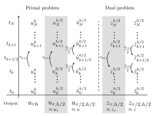
Figure 1: Approximations of the primal and dual solutions. The primal approximations $u_{\tau h}$, $u_{\tau,h/2}$ and $u_{\tau/2,h/2}$ are computed forwards in time and the dual approximations $z_{\tau,h/2}$, $z_{\tau,h/2}$ and $z_{\tau/2,h/2}$ are computed backwards in time with the corresponding spatial meshes and time steps. The computational cost of the algorithm can be reduced by discarding the approximations in the grey columns; see Remark 4.1.

Now let us denote by $\hat{z}\in\mathcal{V}$ a time-reconstruction of the dual solution $z_{\tau/2,h/2}$ (e.g. a piecewise-constant time-reconstruction will be used in numerical applications; see Section 6). By replacing $z$ with $\hat{z}$ in Eq. 32, the estimate of the space-time error in $\mathcal{Q}$ can then be computed as:

(36) $$\mathcal{Q}(u)-\mathcal{Q}(Iu_{\tau h})\approx\mathcal{E}_{\mathrm{st}}:=\mathcal{R}_{0}\left(u_{0}^{h};\hat{z}(0)\right)+\int_{0}^{T}\mathcal{R}_{\mathrm{PDE}}\left(Iu_{\tau h}(t);\hat{z}(t)\right)\,\mathrm{d}t.$$

Replacing $z_{\tau}$ with the computable $z_{\tau,h/2}$ in Eq. 29, we compute the spatial error estimate $\mathcal{E}_{\mathrm{s}}$ as:

(37) $$\mathcal{R}_{\mathrm{s}}(u_{\tau h};z_{\tau})\approx\mathcal{E}_{\mathrm{s}} :=\left(u_{0}^{h/2}-u_{0}^{h},z_{0}^{h/2}\right)+\sum_{k=1}^{N}\tau_{k}\left\langle r_{h}^{k},z_{k}^{h/2}\right\rangle.$$

Finally, replacing $z$ and $z_{\tau}$ with the computable $\hat{z}$ and $z_{\tau,h/2}$ in Eq. 30, respectively, we compute the temporal error estimate $\mathcal{E}_{\mathrm{t}}$ as:

(38) $$\mathcal{R}_{\mathrm{t}}(u_{\tau h},u_{\tau},z,z_{\tau})\approx\mathcal{E}_{\mathrm{t}}:=\left(u_{0}^{h/2}-u_{0}^{h},\hat{z}(0)-z_{0}^{h/2}\right)\\ +\sum_{k=0}^{N-1}\int_{t_{k}}^{t_{k+1}}\bigg{\{}\mathcal{R}_{\mathrm{PDE}}\left(Iu_{\tau h}(t);\hat{z}(t)-z_{k+1}^{h/2}\right)+\left\langle r_{\tau}^{k+1}(t),z_{k+1}^{h/2}\right\rangle\bigg{\}}\,\mathrm{d}t.$$

Remark 4.1 (Reduced-cost implementation).

If one wants to reduce the number of distinct approximations in the error estimates Eq. 36–Eq. 38, the most straightforward strategy is to simply take $u_{\tau,h/2}=u_{\tau/2,h/2}$ and $z_{\tau,h/2}=z_{\tau/2,h/2}$ at concurrent time steps (i.e. $u_{k}^{h/2}=\tilde{u}_{k}^{h/2}$ and $z_{k}^{h/2}=\tilde{z}_{k}^{h/2}$ for $k=0,1,\ldots,N$). In this manner, one only needs to compute $u_{\tau h}$, $u_{\tau/2,h/2}$ and $z_{\tau/2,h/2}$, without the gray columns in Figure 1. More detailed description and examples are given in numerical applications; see Section 6. An even cheaper alternative is to compute higher-order reconstructions using only $u_{\tau h}$ and $z_{\tau h}$; see, Becker and Rannacher [4] for an overview, or coarse-scale adjoints [10].

5 Adaptive algorithm

Our goal is now to design an adaptive algorithm to iteratively increase the accuracy of the numerical solution by using the error estimates. In this section, we first derive error indicators of local contributions that serve as the basis to control adaptive mesh refinement and adaptive time-step selection, and then present the space-time adaptive algorithm.

5.1 Error indicators

To drive space-time adaptivity, the information of the global error estimates has to be localized to time-intervals and spatially-local contributions. To this end, we rewrite the computable error estimates $\mathcal{E}_{\mathrm{st}}$, $\mathcal{E}_{s}$ and $\mathcal{E}_{\mathrm{t}}$ in Eq. 36–Eq. 38 as a sum of their local contributions on each time intervals $[t_{k},t_{k+1}]$, $k=0,1,\ldots,N-1$, respectively. The absolute values of these local contributions are identified as the local indicators, which can directly be used for adaptive time-step selection. For adaptive mesh refinement, the local contributions associated to the spatial discretization error have to be localized further in space. We summarize the result in the following propositions.

Proposition 5.1.

The error estimate $\mathcal{E}_{\mathrm{st}}$, $\mathcal{E}_{\mathrm{t}}$ and $\mathcal{E}_{\mathrm{s}}$ can be bounded from above by

$$|\mathcal{E}_{\mathrm{st}}|\leq\mathcal{E}^{0}_{h\tau}+\sum_{k=0}^{N-1}\mathcal{E}^{k+1}_{h\tau}\qquad\;|\mathcal{E}_{\mathrm{t}}|\leq\mathcal{E}^{0}_{\tau}+\sum_{k=0}^{N-1}\mathcal{E}^{k+1}_{\tau}\qquad\;|\mathcal{E}_{\mathrm{s}}|\leq\mathcal{E}^{0}_{h}+\sum_{k=0}^{N-1}\mathcal{E}^{k+1}_{h}$$

where the local space-time error indicators $\mathcal{E}^{0}_{h\tau}$ and $\mathcal{E}^{k+1}_{h\tau}$ are defined by

(39) $$\mathcal{E}^{0}_{h\tau}:=\Big{|}\mathcal{R}_{0}\left(u_{0}^{h};\hat{z}(0)\right)\Big{|}\qquad\qquad\mathcal{E}^{k+1}_{h\tau}:=\bigg{|}\int_{t_{k}}^{t_{k+1}}\mathcal{R}_{\mathrm{PDE}}\left(Iu_{\tau h}(t);\hat{z}(t)\right)\,\mathrm{d}t\bigg{|},$$

the temporal error indicators $\mathcal{E}^{0}_{\tau}$ and $\mathcal{E}^{k+1}_{\tau}$ are defined by

(40) $$\mathcal{E}^{0}_{\tau}:=\left|\left(u_{0}^{h/2}-u_{0}^{h},\hat{z}(0)-z_{0}^{h/2}\right)\right|$$

(41) $$\begin{split}&\mathcal{E}^{k+1}_{\tau}:=\left|\int_{t_{k}}^{t_{k+1}}\left\{\mathcal{R}_{\mathrm{PDE}}\left(Iu_{\tau h}(t);\hat{z}(t)-z_{k+1}^{h/2}\right)+\left\langle r_{\tau}^{k+1}(t),z_{k+1}^{h/2}\right\rangle\right\}\,\mathrm{d}t\right|\end{split}$$

and the spatial error indicators $\mathcal{E}^{0}_{h}$ and $\mathcal{E}^{k+1}_{h}$ are defined by

(42) $$\mathcal{E}^{0}_{h}:=\Big{|}\left(u_{0}^{h/2}-u_{0}^{h},z_{0}^{h/2}\right)\Big{|}\qquad\qquad\mathcal{E}^{k+1}_{h}:=\Big{|}\tau_{k+1}\langle r_{h}^{k+1},z_{k+1}^{h/2}\rangle\Big{|}.$$

Proof 5.2.

We split the error estimator $\mathcal{E}_{\mathrm{st}}$ Eq. 36 into local space-time error indicators Eq. 39 by

$$\mathcal{E}_{\mathrm{st}} =\mathcal{R}_{0}\left(u_{0}^{h};\hat{z}(0)\right)+\int_{0}^{T}\mathcal{R}_{\mathrm{PDE}}\left(Iu_{\tau h}(t);\hat{z}(t)\right)\,\mathrm{d}t$$

$$=\mathcal{R}_{0}\left(u_{0}^{h};\hat{z}(0)\right)+\sum_{k=0}^{N-1}\int_{t_{k}}^{t_{k+1}}\mathcal{R}_{\mathrm{PDE}}\left(Iu_{\tau h}(t);\hat{z}(t)\right)\,\mathrm{d}t$$

$$\leq\left|\mathcal{R}_{0}\left(u_{0}^{h};\hat{z}(0)\right)\right|+\sum_{k=0}^{N-1}\left|\int_{t_{k}}^{t_{k+1}}\mathcal{R}_{\mathrm{PDE}}\left(Iu_{\tau h}(t);\hat{z}(t)\right)\,\mathrm{d}t\right|$$

Following the same procedure as above, the temporal error estimate $\mathcal{E}_{\mathrm{t}}$ Eq. 38 is localized to the temporal error indicators LABEL:eq:est_time on each time intervals $[t_{k},t_{k+1}]$, $k=0,1,\ldots,N-1$, and the spatial error estimate $\mathcal{E}_{\mathrm{s}}$ Eq. 37 is localized in time to the spatial error indicators Eq. 42.

For spatial adaptivity we consider hierarchical mesh-refinement indicators as explained in [29, Section 4.2]. In addition, let us note that instead of a traditional element-wise marking strategy, we use the function-support marking strategy introduced in [23] (see also [26, 31]).

Remark 5.3.

In general in Eq. 42, one needs to subtract an interpolant of the dual solution, $\Pi z_{\tau h/2}$ from $z_{\tau,h/2}$ to get a sharp spatial indicator. However, this is not needed for hierarchical indicators; see, [29, Section 4.2] for more details.

5.2 The space-time adaptive algorithm

In Algorithm 1, we propose a global space-time adaptive procedure using the above duality-based indicators. The pseudocode consists of three parts: (1) The computation of the primal and dual approximations (comprised of lines 3-8, 9-11 and 13-14), (2) the evaluation of the error estimates (given in lines 12, 15, 18-19 and 23), and (3) the error control (comprised of the remaining lines of Algorithm 1).

Algorithm 1 Duality-based space-time adaptive algorithm

1:Choose a coarse spatial mesh $\mathcal{K}_{0}$ and a coarse time step size $\tau$

2:Initialize a list of spatial mesh $\{\mathcal{K}_{k}\}_{k=1}^{N}$ ($\mathcal{K}_{k}=\mathcal{K}_{0}$) for time steps $\{\tau_{k}\}_{k=1}^{N}$ ($\tau_{k}=\tau$)

3:while the maximal error estimate $Max$ $>$ tol do

4:    for $k\in\{1,2,\ldots,N\}$ do

5:        Compute $u_{\tau h}$ in $\mathcal{K}_{k}$ with $\tau_{k}$

6:        Compute $u_{\tau,h/2}$ in $\mathcal{K}^{h/2}_{k}$ with $\tau_{k}$

7:        Compute $u_{\tau/2,h/2}$ in $\mathcal{K}^{h/2}_{k}$ with $\tau_{k}/2$

8:        $t=t+\tau_{k}$

9:    end for

10:    for $k\in\{N,N-1,\ldots,1\}$ do

11:        Compute $z_{\tau,h/2}$ in $\mathcal{K}^{h/2}_{k-1}$ with $\tau_{k}$

12:        Compute $z_{\tau/2,h/2}$ in $\mathcal{K}^{h/2}_{k-1}$ with $\tau_{k}/2$

13:        Estimate the error contribution $\mathcal{E}^{k}_{h\tau}$

14:        $t=t-\tau_{k}$

15:    end for

16:    Estimate the initial error contribution $\mathcal{E}^{0}_{h\tau}$

17:    Compute the maximal error contribution for the whole time period $Max=\max\{\mathcal{E}^{0}_{h\tau},\ldots,\mathcal{E}^{N}_{h\tau}\}$

18:    while $|\mathcal{E}^{k}_{h\tau}|>\theta\,|Max|$ do

19:        Estimate the local temporal error indicator $\mathcal{E}^{k}_{\tau}$

20:        Estimate the local spatial error indicator $\mathcal{E}^{k}_{h}$

21:        if $\mathcal{E}^{k}_{\tau}\geq\mathcal{E}^{k}_{h}$ then

22:           Refine the time step $\tau_{k}$ by half

23:        else

24:           Estimate $\mathcal{E}^{k}_{i}$ for the mesh $\mathcal{K}_{k}$

25:           Refine the mesh $\mathcal{K}_{k}$ by using hierarchical refinement strategy and maximum strategy with parameter $\lambda$

26:        end if

27:    end while

28:end while

Within the adaptive procedure, the error control is built on a two-step approach. First, in lines 16-17 of the pseudocode we apply the maximum marking strategy (following Babuška and Vogelius [3]) with fraction $\theta\in[0,1]$ on space-time error indicators $\{\mathcal{E}^{k}_{h\tau}\}_{k=0}^{N}$ to globally select time steps $\{k^{\prime}\}$ (i.e. $|\mathcal{E}^{k^{\prime}}_{h\tau}|\geq\theta\,\max\{|\mathcal{E}^{0}_{h\tau}|,|\mathcal{E}^{1}_{h\tau}|,\ldots,|\mathcal{E}^{N}_{h\tau}|\}$), which contain the largest error contributions throughout the time period. Second, in line 20 we locally check the leading causes of the error at the targeted time steps $\{k^{\prime}\}$, whether from the spatial error or from the temporal error. An example of this is shown and explained in Figure 2. The figure on the left indicates the time steps $\{k^{\prime}\}$, where the major error contributions are located. Then, if the spatial indicator $\mathcal{E}^{k^{\prime}}_{h}$ is larger than the temporal indicator $\mathcal{E}^{k^{\prime}}_{\tau}$, the spatial mesh is targeted for refinement according to the mesh indicators $\mathcal{E}_{i}^{k^{\prime}}$; see Figure 2 (center). Otherwise, the time step size $\tau_{k^{\prime}}$ is marked and reduced by half ; see Figure 2 (right).

The adaptive spatial mesh refinement is also based on a maximum marking strategy. The nodes $\{i^{\prime}\}$ are marked for which their mesh-refinement indicators are at least a fraction $\lambda\in[0,1]$ of the maximal mesh indicator (i.e. $|\mathcal{E}_{i^{\prime}}^{k}|\geq\lambda\max\{|\mathcal{E}_{0}^{k}|,\ldots,|\mathcal{E}_{M}^{k}|\}$). The addition of the basis function on selected nodes is performed using hierarchical refinement for finite element methods [22, 23, 26, 31]. Moreover, instead of projection, we introduce a common refinement to transfer the solution from one mesh to another without loss of accuracy in any quadrature approximations.

Remark 5.4.

A standard adaptive algorithm for time-dependent problems starts with an initial coarse mesh, and proceeds sequentially. Based on the mesh for the current time step, a new space mesh is generated for each new time step. Such a sequential procedure commonly uses residual-based error estimates in space which only contain information at the current time step. Duality-based error estimates, on the contrary, contain the entire evolution history of the error dependence implicitly via the dual solution.

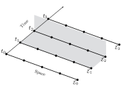
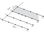
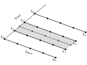
Figure 2: Adaptive mesh refinement. Left: assume that $\mathcal{E}^{2}_{h\tau}=\max\{\mathcal{E}^{0}_{h\tau},\mathcal{E}^{1}_{h\tau},\mathcal{E}^{2}_{h\tau},\mathcal{E}^{3}_{h\tau}\}$, i.e., the second time step $[t_{1},t_{2}]$ is targeted as the largest error contribution throughout the time period. Middle: If the spatial indicator $\mathcal{E}^{2}_{h}$ is larger than the temporal indicator $\mathcal{E}^{2}_{\tau}$, the space mesh is targeted to refine according to the mesh indicators $\mathcal{E}^{2}_{i}$. Right: If the spatial indicator is smaller than the temporal indicator, the time step size is cut into half.

6 Applications

In this section, we give two examples of problems which fit into the abstract framework introduced in Section 2: the nonlinear Allen–Cahn equation and the linear heat equation (as a special case of the Allen–Cahn equation). We numerically investigate the performance of the duality-based error estimates and the proposed adaptive algorithm.

Let us point out that the abstract framework easily accommodates other applications, for example, systems of parabolic equations; see [36, Section 6.3] for the application to a phase-field tumor-growth system.

6.1 Allen–Cahn equation

We subject the (forced) Allen–Cahn equation, $\partial_{t}u-\Delta u+\epsilon^{-2}\psi^{\prime}(u)=f(t)$, to homogeneous Neumann boundary conditions. We choose the function spaces as $\mathcal{V}=H^{1}(\Omega)$, $\mathcal{V}^{*}=[H^{1}(\Omega)]^{*}$ and set $\mathcal{B}(u,v)=(\nabla u,\nabla v)$, $\mathcal{N}(u;v)=\frac{1}{\epsilon^{2}}\left(\psi^{\prime}(u),v\right)$ in Eq. 1, where $\epsilon$ is a parameter that controls the thickness of the diffuse interface (typical in phase-field models), and the nonlinear double-well function $\psi(u)$ is defined as (a standard truncated quartic polynomial)

(43) $$\psi(u):=\left\{\begin{array}[]{ll}(u+1)^{2}&u<-1\\[8.0pt] {\displaystyle{\frac{1}{4}(u^{2}-1)^{2}}}&u\in[-1,1]\\[8.0pt] (u-1)^{2}&u>1.\end{array}\right.$$

Then, we obtain the weak form of the Allen–Cahn equation is: Find $u\in\mathcal{W}_{u^{0}}:=\left\{v\in L^{2}(0,T;\mathcal{V}),\partial_{t}v\in L^{2}\left(0,T;\mathcal{V}^{*}\right):v(0)=u^{0}\right\}$ such that $\forall v\in L^{2}(0,T;H^{1}(\Omega))$

(44) $$\int_{0}^{T}\left(\left\langle\partial_{t}u,v\right\rangle+(\nabla u,\nabla v)+\frac{1}{\epsilon^{2}}\left(\psi^{\prime}(u),v\right)\right)\mathrm{d}t=\int_{0}^{T}\left\langle f,v\right\rangle\mathrm{d}t.$$

In our setting the IMEX scheme for Eq. 44 leads to the energy-stable time-stepping scheme introduced in [17]: find $u_{k+1}\in H^{1}(\Omega)$ such that $\forall v\in H^{1}(\Omega)$

(45) $$\left(\frac{u_{k+1}-u_{k}}{\tau_{k+1}},v\right)+(\nabla u_{k+1},\nabla v)+\frac{1}{\epsilon^{2}}\left(\psi^{\prime}_{c}(u_{k+1}),v\right)-\frac{1}{\epsilon^{2}}\left(\psi^{\prime}_{e}(u_{k}),v\right)=\left(\bar{f}_{k+1},v\right)$$

for $k=0,1,\ldots,N-1$, where the initial condition is $(u_{0},v)=(u^{0},v)$, $\forall v\in L^{2}(\Omega)$, and where we choose $\bar{f}_{k+1}=\frac{1}{\tau_{k+1}}\int_{t_{k}}^{t_{k+1}}f(\cdot,t)\,\mathrm{d}t$. In particular, for a splitting of $\psi$ with a quadratic convex part, the resulting system is linear, for example:

$$\psi=\psi_{c}-\psi_{e}=\left\{\begin{array}[]{ll}{\displaystyle{\left(u^{2}+\frac{1}{4}\right)-\left(-2u-\frac{3}{4}\right)}}&u<-1\\ {\displaystyle{\left(u^{2}+\frac{1}{4}\right)-\left(\frac{3}{2}u^{2}-\frac{1}{4}u^{4}\right)}}&u\in[-1,1]\\ {\displaystyle{\left(u^{2}+\frac{1}{4}\right)-\left(2u-\frac{3}{4}\right)}}&u>1.\end{array}\right.$$

We then have the full discretization: find $u_{k+1}^{h}\in\mathcal{S}^{h,1}_{k+1}$ such that $\forall v^{h}\in\mathcal{S}^{h,1}_{k+1}$

(46) $$\!\left(\frac{u_{k+1}^{h}-u_{k}^{h}}{\tau_{k+1}},v^{h}\right)+(\nabla u_{k+1}^{h},\nabla v^{h})\\ +\frac{1}{\epsilon^{2}}\left(\psi^{\prime}_{c}(u^{h}_{k+1}),v^{h}\right)-\frac{1}{\epsilon^{2}}\left(\psi^{\prime}_{e}(u^{h}_{k}),v^{h}\right)=\left(\bar{f}_{k+1},v^{h}\right)$$

for $k=0,1,\ldots,N-1$, where the initial condition is $(u^{h}_{0},v^{h})=(u^{0},v^{h})$, $\forall v^{h}\in\mathcal{S}^{h,1}_{0}$.

According to the definition of $\mathcal{N}^{s}$ in Eq. 3, we can explicitly write the mean-value linearization of $\psi^{\prime}(u)$ in terms of $u$ and $\hat{u}$:

$$\psi^{\prime s}(u,\hat{u})=\int_{0}^{1}\psi^{\prime\prime}(su+(1-s)\hat{u})\mathrm{d}s,$$

although, because of its piecewise definition Eq. 43, this is an elaborate expression. For example, for $u,\hat{u}>1$ or $u,\hat{u}<-1$, we have $\psi^{\prime s}(u,\hat{u})=2$, and for $u,\hat{u}\in[-1,1]$, we have $\psi^{\prime s}(u,\hat{u})=u^{2}+\hat{u}^{2}+u\hat{u}-1$.

Then, by setting $\mathcal{N}^{s}(u,\hat{u};w,z)=\frac{1}{\epsilon^{2}}\big{(}\psi^{\prime s}(u,\hat{u})z,w\big{)}$ in Eq. 5, the dual problem reads: find $z\in\mathcal{W}^{\bar{q}}:=\left\{v\in L^{2}(0,T;\mathcal{V}),\partial_{t}v\in L^{2}\left(0,T;\mathcal{V}^{*}\right):v(T)=\bar{q}\right\}$ such that $\forall w\in L^{2}(0,T;H^{1}(\Omega))$

(47) $$\int_{0}^{T}\Big{(}\left\langle-\partial_{t}z,w\right\rangle+(\nabla z,\nabla w)+\frac{1}{\epsilon^{2}}\left(\psi^{\prime s}(u,\hat{u})z,w\right)\Big{)}\,\mathrm{d}t=\int_{0}^{T}(q,w)\,\mathrm{d}t,$$

And the IMEX time-discrete dual problem, based on Eq. 23-Eq. 25, is defined by: find $z_{k}\in H^{1}(\Omega)$, $k=0,1,\ldots,N$, such that

(48) $$-\left(\frac{z_{1}-z_{0}}{\tau_{1}},w\right)-\frac{1}{\epsilon^{2}}\left(\psi^{\prime s}_{e}(u_{0},u_{0}^{h})z_{1},w\right)=(q_{0},w)\quad\forall w\in H^{1}(\Omega)$$

and for $k=1,2,\ldots,N-1$:

(49) $$-\Big{(}\frac{z_{k+1}-z_{k}}{\tau_{k}},w\Big{)}+(\nabla z_{k},\nabla w)+\frac{1}{\epsilon^{2}}\left(\psi^{\prime s}_{c}(u_{k},u_{k}^{h})z_{k},w\right)\\ -\frac{\tau_{k+1}}{\tau_{k}}\frac{1}{\epsilon^{2}}\left(\psi^{\prime s}_{e}(u_{k},u_{k}^{h})z_{k+1},w\right)=(q_{k},w)\qquad\forall w\in H^{1}(\Omega)$$

where the terminal condition is

(50) $$\left(z_{N},w\right)+\tau_{N}(\nabla z_{N},\nabla w)+\tau_{N}\frac{1}{\epsilon^{2}}\left(\psi^{\prime s}_{c}(u_{N},u_{N}^{h})z_{N},w\right)\\ =(\bar{q},w)+\tau_{N}(q_{N},w)\qquad\forall w\in H^{1}(\Omega)$$

with $q_{k}$, $k=0,1,\ldots,N$ defined in Lemma 3.4. Note that for our choice of $\psi_{c}$, the derivative $\psi^{\prime s}_{c}$ reduces to a constant. The main results of Section 3 hold, as shown in the following corollary.

Corollary 6.1 (Decomposed error representation for Allen–Cahn equation).

The following error representation holds

$$\begin{split}\mathcal{Q}(u)-\mathcal{Q}(Iu_{\tau h})&=\left(z(0),u^{0}-u_{0}^{h}\right)+\sum_{k=0}^{N-1}\int_{t_{k}}^{t_{k+1}}\bigg{\{}\left\langle f(t),z(t)\right\rangle-\big{(}\partial_{t}Iu_{\tau h}(t),z(t)\big{)}\\ &\quad-\big{(}\nabla Iu_{\tau h}(t),\nabla z(t)\big{)}-\frac{1}{\epsilon^{2}}\big{(}\psi^{\prime}(Iu_{\tau h}(t)),z(t)\big{)}\bigg{\}}\,\mathrm{d}t\end{split}$$

$$=\mathcal{R}_{\mathrm{s}}(u_{\tau h};z_{\tau})+\mathcal{R}_{\mathrm{t}}(u_{\tau h},u_{\tau},z,z_{\tau}),$$

where the spatial error representation reduces to

$$\mathcal{R}_{\mathrm{s}}(u_{\tau h};z_{\tau})=(z_{0},u^{0}-u_{0}^{h})+\sum_{k=0}^{N-1}\tau_{k+1}\left\{\left(\bar{f}_{k+1},z_{k+1}\right)-\left(\frac{u^{h}_{k+1}-u^{h}_{k}}{\tau_{k+1}},z_{k+1}\right)\right.\\ \left.-(\nabla z_{k+1},\nabla u_{k+1}^{h})-\frac{1}{\epsilon^{2}}\left(\psi^{\prime}_{c}(u_{k+1}^{h}),z_{k+1}\right)+\frac{1}{\epsilon^{2}}\left(\psi^{\prime}_{e}(u_{k}^{h}),z_{k+1}\right)\right\}$$

and the temporal error representation reduces to

$$\begin{split}&\mathcal{R}_{\mathrm{t}}(u_{\tau h},u_{\tau},z,z_{\tau})=\left(z(0)-z_{0},u^{0}-u_{0}^{h}\right)+\sum_{k=0}^{N-1}\int_{t_{k}}^{t_{k+1}}\bigg{\{}\left\langle f(t),z(t)-z_{k+1}\right\rangle\\ &\quad-\left(\frac{u^{h}_{k+1}-u^{h}_{k}}{\tau_{k+1}},z(t)-z_{k+1}\right)-(\nabla Iu_{\tau h}(t),\nabla z(t))+(\nabla u_{k+1}^{h},\nabla z_{k+1})\\ &\quad-\frac{1}{\epsilon^{2}}\big{(}\psi^{\prime}(Iu_{\tau h}(t)),z(t)\big{)}+\frac{1}{\epsilon^{2}}\left(\psi^{\prime}_{c}(u_{k+1}^{h}),z_{k+1}\right)-\frac{1}{\epsilon^{2}}\left(\psi^{\prime}_{e}(u_{k}^{h}),z_{k+1}\right)\bigg{\}}\,\mathrm{d}t.\end{split}$$

Proof 6.2.

The result simply follows from Theorem 3.9 applied to Eq. 44–Eq. 50.

6.2 Computable error indicator

Let $u_{\tau h}=\{u_{k}^{h/2}\}_{k=0}^{N}$ denote the solution of the fully-discrete primal problem Eq. 46 using time-step sizes $\{\tau_{k}\}_{k=1}^{N}$ and FE spaces $\{\mathcal{S}^{h,1}_{k}\}_{k=0}^{N}$, and let $u_{\tau,h/2}=\{u_{k}^{h/2}\}_{k=0}^{N}$ denote the solution of Eq. 46 using time-step sizes $\{\tau_{k}\}_{k=1}^{N}$ and enriched FE spaces $\{\mathcal{S}^{h/2,1}_{l}\}_{l=0,1/2,\ldots,N}$. Replacing $u_{\tau}$ with the computable $u_{\tau,h/2}$ in Eq. 48-Eq. 50, we obtain the full discretization of the dual problem using enriched FE spaces: find $z_{k}^{h/2}\in\mathcal{S}^{h/2,1}_{k}$, $k=0,1,\ldots,N$, such that

(51) $$-\left(\frac{z_{1}^{h/2}-z_{0}^{h/2}}{\tau_{1}},w^{h/2}\right)-\frac{1}{\epsilon^{2}}\left(\psi^{\prime s}_{e}(u_{0}^{h/2},u_{0}^{h})z_{1}^{h/2},w^{h/2}\right)=(q_{0},w^{h/2})\quad\forall w^{h/2}\in\mathcal{S}^{h/2,1}_{0}$$

and for $k=1,2,\ldots,N-1$:

(52) $$-\Bigg{(}\frac{z_{k+1}^{h/2}-z_{k}^{h/2}}{\tau_{k}},w^{h/2}\Bigg{)}+(\nabla z_{k}^{h/2},\nabla w^{h/2})+\frac{1}{\epsilon^{2}}\left(\psi^{\prime s}_{c}(u_{k}^{h/2},u_{k}^{h})z_{k}^{h/2},w^{h/2}\right)\\ -\frac{\tau_{k+1}}{\tau_{k}}\frac{1}{\epsilon^{2}}\left(\psi^{\prime s}_{e}(u_{k}^{h/2},u_{k}^{h})z_{k+1},w^{h/2}\right)=(q_{k},w^{h/2})\qquad\forall w^{h/2}\in\mathcal{S}^{h/2,1}_{k}$$

where the terminal condition is

(53) $$\left(z_{N}^{h/2},w^{h/2}\right)+\tau_{N}(\nabla z_{N-1}^{h/2},\nabla w^{h/2})+\frac{\tau_{N}}{\epsilon^{2}}\left(\psi^{\prime s}_{c}(u_{N}^{h/2},u_{N}^{h})z_{N},w^{h/2}\right)\\ =\tau_{N}(q_{N},w^{h/2})+(\bar{q},w^{h/2})\qquad\forall w^{h/2}\in\mathcal{S}^{h/2,1}_{N}$$

We denote by $z_{\tau,h/2}=\{z_{k}^{h/2}\}_{k=0}^{N}$ the solution of Eq. 51-Eq. 53. To get $z_{\tau/2,h/2}$, we first compute the space-time enriched approximation $u_{\tau/2,h/2}=\{\tilde{u}_{l}^{h/2}\}_{l=0,1/2,\ldots,N}$ of the primal problem using half time-step sizes $\{\tau_{1}/2,\tau_{1}/2,\tau_{2}/2,\tau_{2}/2,\ldots,\tau_{N}/2,\tau_{N}/2\}$ and enriched FE spaces $\{\mathcal{S}^{h/2,1}_{l}\}_{l=0,1/2,\ldots,N}$. Then, replacing $u_{\tau}$ with $u_{\tau/2,h/2}$ in Eq. 48-Eq. 50, we compute the space-time enriched approximation $z_{\tau/2,h/2}=\{\tilde{z}_{l}^{h/2}\}_{l=0,1/2,\ldots,N}$ using the same time-step sizes and FE spaces as $u_{\tau/2,h/2}$.

In the numerical examples for the Allen–Cahn equation in Section 6.3 we compute $u_{\tau,h/2}$ and $z_{\tau,h/2}$ directly by taking $u_{\tau,h/2}=u_{\tau/2,h/2}$ and $z_{\tau,h/2}=z_{\tau/2,h/2}$ at concurrent time steps as in Remark 4.1, and consider a piecewise-constant time-reconstruction $\hat{z}$ of $z_{\tau/2,h/2}$ for each time interval $[t_{k},t_{k+1})$, $k=0,1,\ldots,N-1$, i.e.

$$\hat{z}(t)=\tilde{z}_{k}^{h/2}\quad\text{for }t\in[t_{k},t_{k+1/2}),\qquad\hat{z}(t)=\tilde{z}_{k+1/2}^{h/2}\quad\text{for }t\in[t_{k+1/2},t_{k+1}).$$

According to Eq. 36 and Eq. 39-Eq. 42, we then get the following global space-time error estimate:

(54) $$\mathcal{E}_{\mathrm{st}}=\left(\hat{z}(0),u_{0}^{h/2}-u_{0}^{h}\right)+\sum_{k=0}^{N-1}\int_{t_{k}}^{t_{k+1}}\left\{\left\langle f(t),\hat{z}(t)\right\rangle-\left(\frac{u^{h}_{k+1}-u^{h}_{k}}{\tau_{k+1}},\hat{z}(t)\right)\right.\\ \left.-\big{(}\nabla Iu_{\tau h}(t),\nabla\hat{z}(t)\big{)}-\frac{1}{\epsilon^{2}}\big{(}\psi^{\prime}(Iu_{\tau h}(t)),\hat{z}(t)\big{)}\right\}\,\mathrm{d}t$$

and the local error indicators

$$\mathcal{E}^{k+1}_{h\tau}\!= \Bigg{|}\int_{t_{k}}^{t_{k+1}}\!\Bigg{\{}\left\langle f(t),\hat{z}(t)\right\rangle-\left(\frac{u^{h}_{k+1}-u^{h}_{k}}{\tau_{k+1}},\hat{z}(t)\right)-(\nabla Iu_{\tau h}(t),\nabla\hat{z}(t))$$

$$-\frac{1}{\epsilon^{2}}\big{(}\psi^{\prime}(Iu_{\tau h}(t)),\hat{z}(t)\big{)}\Bigg{\}}\,\mathrm{d}t\Bigg{|}$$

$$\mathcal{E}_{\tau}^{k+1}\!= \Bigg{|}\int_{t_{k}}^{t_{k+1}}\!\Bigg{\{}\left\langle f(t),\hat{z}(t)-\tilde{z}^{h/2}_{k+1}\right\rangle$$

$$-\left(\frac{u^{h}_{k+1}-u^{h}_{k}}{\tau_{k+1}},\hat{z}(t)-\tilde{z}_{k+1}^{h/2}\right)-\big{(}\nabla Iu_{\tau h}(t),\nabla\hat{z}(t)\big{)}+(\nabla u_{k+1}^{h},\nabla\tilde{z}_{k+1}^{h/2})$$

$$-\frac{1}{\epsilon^{2}}\big{(}\psi^{\prime}(Iu_{\tau h}(t)),\hat{z}(t)\big{)}+\frac{1}{\epsilon^{2}}\left(\psi^{\prime}_{c}(u_{k+1}^{h}),\tilde{z}_{k+1}^{h/2}\right)-\frac{1}{\epsilon^{2}}\left(\psi^{\prime}_{e}(u_{k}^{h}),\tilde{z}_{k+1}^{h/2}\right)\Bigg{\}}\,\mathrm{d}t\Bigg{|}$$

$$\mathcal{E}_{h}^{k+1}\!= \Bigg{|}\tau_{k+1}\Bigg{\{}\left(\bar{f}_{k+1},\tilde{z}^{h/2}_{k+1}\right)-\left(\frac{u^{h}_{k+1}-u^{h}_{k}}{\tau_{k+1}},\tilde{z}_{k+1}^{h/2}\right)-(\nabla\tilde{z}_{k+1}^{h/2},\nabla u_{k+1}^{h})$$

$$-\frac{1}{\epsilon^{2}}\big{(}\psi^{\prime}_{c}(u_{k+1}^{h}),\tilde{z}_{k+1}^{h/2}\big{)}+\frac{1}{\epsilon^{2}}\big{(}\psi^{\prime}_{e}(u_{k}^{h}),\tilde{z}_{k+1}^{h/2}\big{)}\Bigg{\}}\Bigg{|}$$

for $k=0,1,\ldots,N-1$ and $i=0,1,\ldots,M_{k}$. And since $z_{0}^{h/2}=\hat{z}(0)=\tilde{z}_{0}^{h/2}$,

$$\mathcal{E}_{h\tau}^{0}=\mathcal{E}_{h}^{0}=\left(u_{0}^{h/2}-u_{0}^{h},\tilde{z}_{0}^{h/2}\right)$$

$$\mathcal{E}_{\tau}^{0}=0.$$

Remark 6.3.

For the linear heat equation, $\partial_{t}u-\Delta u=f$, note that the dual problem and the computable error indicators are easily obtained from the above results by neglecting the nonlinear terms $\psi^{\prime}_{e}$ and $\psi^{\prime}_{c}$.

6.3 Numerical results

In the following numerical experiments, we investigate the efficiency of the duality-based error estimates and the performance of the proposed adaptive algorithm. The results will be demonstrated in three parts. In the first part, we illustrate the consistency of the dual time scheme Eq. 48–Eq. 50 since we introduced a non-standard IMEX time-discrete dual problem Eq. 23–Eq. 25 which contains a nonstandard coefficient $\tau_{k+1}/\tau_{k}$. The second part is on the convergence of error estimate $\mathcal{E}_{\mathrm{st}}$ under uniform refinements for the nonlinear Allen–Cahn equation. In the third part, we apply the proposed duality-based adaptive algorithm to the linear heat equation and the nonlinear Allen–Cahn equation. We compare our adaptive result for the heat equation with the sequential-in-time adaptive algorithm (specifically for the heat equation) of Verfürth stated in [33, Sec. 6.8]. For the Allen–Cahn equation, we compare our adaptive results with uniform space-time refinements.

Consistency test

We begin with verifying numerically that the special IMEX time scheme of the dual problem Eq. 23-Eq. 25 is first-order accurate in time with respect to refinements of uniform initial time steps (i.e. $\tau_{k+1}/\tau_{k}=1$) and, in particular, nonuniform initial time steps (i.e. $\tau_{k+1}/\tau_{k}\neq 1$). Here, the Allen–Cahn equation is considered in 1D on the domain $\Omega=(-3,3)$ with parameter $\epsilon=1$. The spatial mesh is composed of $256$ elements along the axis. We consider a manufactured solution which oscillates in time:

$$z(\mathbf{x},t)=e^{-10x^{2}+\sin{t}}$$

The convergence results are presented on a double logarithmic scale in Figure 3. Figure 3a is the convergence of the error in $L^{2}$ norm at time $T$ based on time-step refinements using uniform initial time steps $\{\tau_{k}\}_{k=1}^{5}=\{0.1,0.1,0.1,0.1,0.1\}$, and Figure 3b uses nonuniform initial time steps $\{\tau_{k}\}_{k=1}^{5}=\{2\cdot 10^{-2}(3k+1)\}_{k=4}^{0}=\{0.26,0.2,0.14,0.08,0.02\}$. For both uniform and nonuniform initial time steps, the observed rates are close to 1, which demonstrates that Eq. 23-Eq. 25 is a first-order time-accurate scheme.

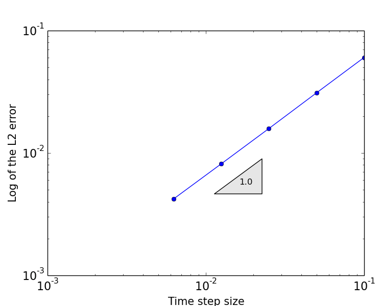
(a) Uniform

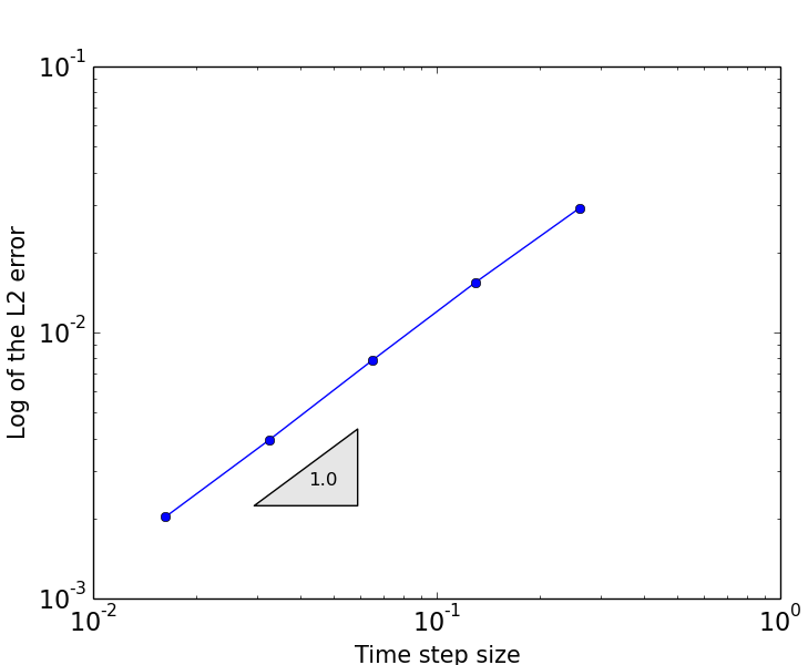
(b) Nonuniform

Figure 3: Accuracy test for dual IMEX scheme: (a) log of the $L^{2}$ norm of the error at time $T$ versus time step size (uniform initial time steps); (b) log of the $L^{2}$ norm of the error at time $T$ versus maximum time step size (nonuniform initial time steps)

Effectivity test

In this numerical experiment, we consider the Allen–Cahn equation with an exact solution

$$u(\mathbf{x},t)=\sin(\pi x)\,\sin(\pi y)\,e^{-t}$$

on the domain $\Omega=(0,1)\times(0,1)$ where $\epsilon=1$. We suppose that we are interested in the error at final time $T$, i.e., in (2) we take $q=0$ and $\bar{q}=u(T)-Iu_{\tau h}(T)$ (which is approximated in the computations by $\bar{q}\approx\tilde{u}_{N}^{h/2}-u_{N}^{h}$, see Section 4). The error of interest is thus $\mathcal{Q}(u)-\mathcal{Q}(Iu_{\tau h})=\|u(T)-Iu_{\tau h}(T)\|_{L^{2}(\Omega)}^{2}=\|u(T)-u_{N}^{h}\|_{L^{2}(\Omega)}^{2}$.

To investigate the error estimate with respect to the spatial discretization, temporal discretization and space-time discretization, we compute $\mathcal{E}_{\mathrm{st}}$ according to Eq. 54 under uniform spatial refinement, uniform temporal refinement and uniform space-time refinement, respectively. In view of the nonstandard time discretization scheme for the dual problem, we also investigate the accuracy of the error estimate $\mathcal{E}_{\mathrm{st}}$ with respect to uniform and nonuniform initial time step sizes. Table 1 presents the convergence of $\mathcal{E}_{\mathrm{st}}$ under uniform spatial refinement for a sufficiently small time step size ($\tau_{k}=1e-4$). For uniform initial time steps $\{\tau_{k}\}_{k=1}^{4}=\{0.05,0.05,0.05,0.05\}$, the left side of Table 2 shows the convergence of $\mathcal{E}_{\mathrm{st}}$ under uniform temporal refinement for a sufficiently fine spatial mesh ($128\times 128$ elements) and the left side of Table 3 shows the convergence under uniform space-time refinements. For nonuniform initial time steps $\{\tau_{k}\}_{k=1}^{4}=\{0.08,0.06,0.04,0.02\}$, the convergence result for uniform temporal refinement with a sufficiently fine spatial mesh is presented on the right side of Table 2, and the convergence result for uniform space-time refinements is presented on the right side of Table 3. The effectivity results for different refinements are also presented in the two tables.

$M$	$\mathcal{Q}(u)-\mathcal{Q}(Iu_{\tau h})$	$\mathcal{E}_{\mathrm{st}}$	Effectivity
16	0.0003046	0.0002871	0.943
64	1.711e-05	1.606e-05	0.939
256	1.041e-06	9.756e-07	0.938
1024	6.458e-08	6.054e-08	0.937
4096	4.028e-09	3.776e-09	0.937

Table 1: Effectivity of error estimate Eq. 54 under spatial refinement

	Uniform initial time steps			Nonuniform initial time steps
$N$	$\mathcal{Q}(u)-\mathcal{Q}(Iu_{\tau h})$	$\mathcal{E}_{\mathrm{st}}$	Eff	$\mathcal{Q}(u)-\mathcal{Q}(Iu_{\tau h})$	$\mathcal{E}_{\mathrm{st}}$	Eff
4	0.0001378	5.893e-05	0.428	0.0001058	4.773e-05	0.451
8	3.584e-05	1.659e-05	0.463	2.612e-05	1.253e-05	0.480
16	8.918e-06	4.272e-06	0.479	6.247e-06	3.054e-06	0.489
32	2.130e-06	1.032e-06	0.484	1.444e-06	7.063e-07	0.489
64	4.778e-07	2.303e-07	0.482	3.122e-07	1.507e-07	0.483

Table 2: Effectivity of error estimate Eq. 54 under temporal refinement with uniform initial time steps and nonuniform initial time steps

	Uniform initial time steps			Nonuniform initial time steps
$M\times N$	$\mathcal{Q}(u)-\mathcal{Q}(Iu_{\tau h})$	$\mathcal{E}_{\mathrm{st}}$	Eff	$\mathcal{Q}(u)-\mathcal{Q}(Iu_{\tau h})$	$\mathcal{E}_{\mathrm{st}}$	Eff
256	6.061e-05	2.583e-05	0.426	4.184e-05	2.013e-05	0.481
2048	2.471e-05	1.086e-05	0.440	1.651e-05	7.581e-06	0.459
16384	7.926e-06	3.717e-06	0.469	5.295e-06	2.534e-06	0.479
131072	2.233e-06	1.082e-06	0.485	1.491e-06	7.299e-07	0.489

Table 3: Effectivity of error estimate Eq. 54 under space-time refinement with uniform initial time steps and nonuniform initial time steps

From all the results of Table 1–Table 3, we observe that the error and the estimate converge with the same order under various refinements. The effectivity indices are always between $0.4$ and $1$, and seem to converge to a constant. This indicates the asymptotic effectivity of the error estimate.

Adaptivity test for the linear heat equation: Clockwise moving source

Let $\Omega=(0,1)\times(0,2)$. We take the example from Asner, Tavener and Kay [2] by choosing the right hand side and the initial and the boundary condition so that the exact solution is given by

$$u(\mathbf{x},t)=\exp(-100(x-0.5-0.25\sin(\pi t))^{2}-100(y-1-0.5\cos(\pi t))^{2})$$

which is an exponential peak moving clockwise inside the domain, see Figure 4. We set up the final time $T=0.5$ and $\theta=\lambda=0.8$, and start the adaptive procedure with a uniform mesh containing $4\times 8$ elements and $10$ equally distributed time steps (i.e. $\tau=0.05$). We aim to minimize the error at final time $T$, i.e., as before, $\mathcal{Q}(u)-\mathcal{Q}(Iu_{\tau h})=\|u(T)-Iu_{\tau h}(T)\|_{L^{2}(\Omega)}^{2}=\|u(T)-u_{N}^{h}\|_{L^{2}(\Omega)}^{2}$. For the sequential adaptive algorithm, we choose an initial coarse mesh with $4\times 8$ elements and an initial $\tau=0.01$.

Exact
Sequential
Duality-based

(a)

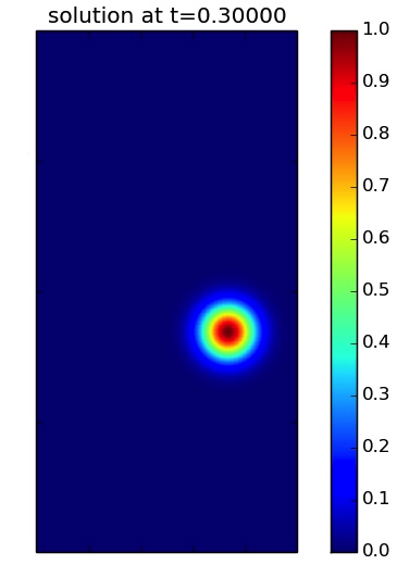
(b)

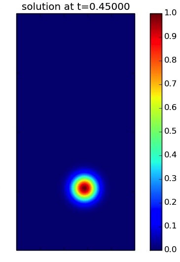
(c)

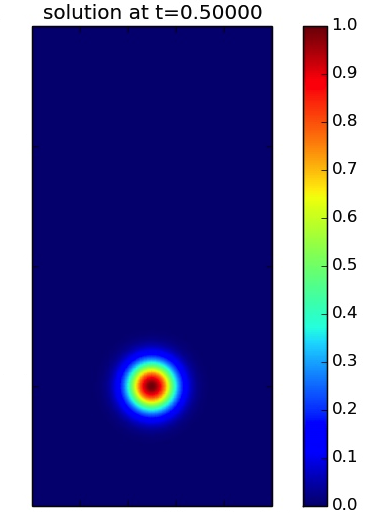
(d)

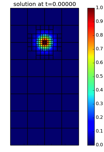
(e)

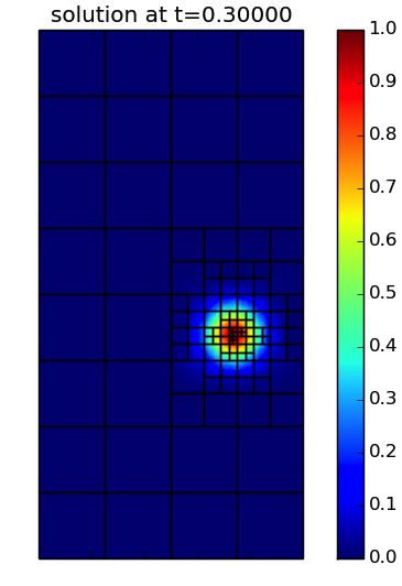
(f)

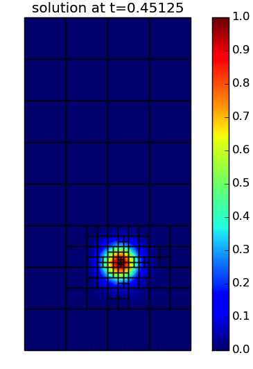
(g)

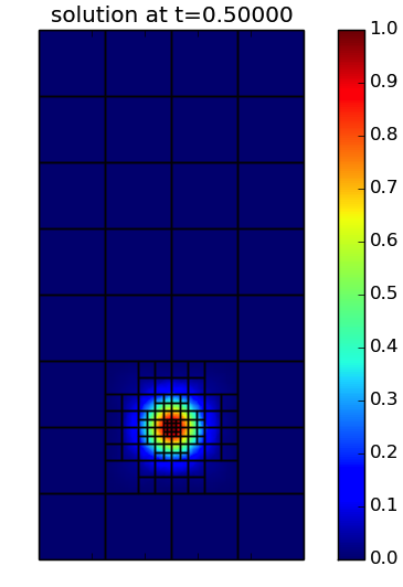
(h)

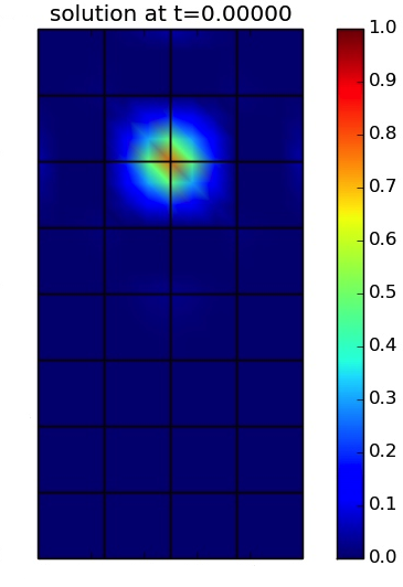
(i) $t=0.0$

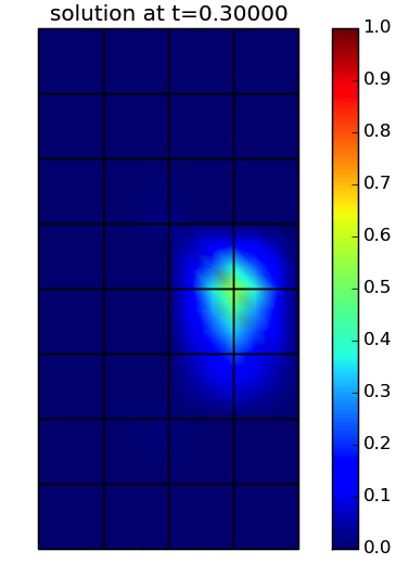
(j) $t=0.3$

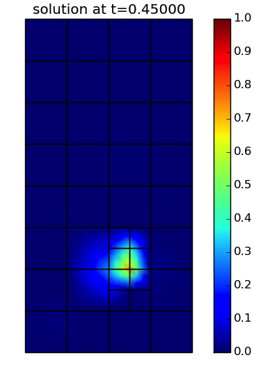
(k) $t=0.45$

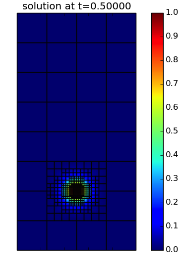
(l) $t=0.5$

Figure 4: Snapshot of the exact solution (first row), the sequential adaptive solution with the computational mesh (second row) and the duality-based adaptive solution with the computational mesh (third row) at several time points

In Figure 4, we show a comparison of the results obtained by the sequential adaptive algorithm and our duality-based adaptive algorithm. The first row corresponds to the exact solution. The second and third row are the snapshots of adaptively refined meshes with corresponding approximations by using the two adaptive algorithms. Figure 6 illustrates the various time steps over time for the two adaptive algorithms. A comparison of the convergence of the error is shown in Figure 6 where ‘Total dof’ refers to total number of degrees of freedom, $\sum_{k=0}^{N}M_{k}$.

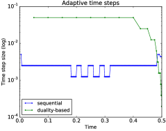
Figure 5: Adaptive time step refinement for the sequential adaptive algorithm and the non-sequential duality-based adaptive algorithm

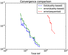
Figure 6: Convergence comparison between the sequential adaptive algorithm and the non-sequential duality-based adaptive algorithm

From these results, it can be seen that the spatial and temporal refinements of the sequential adaptive algorithm focus on tracing the movement of the Gaussian shaped peak of the solution in the space-time domain. In contrast, since our duality-based adaptive algorithm targets the $L^{2}$ norm of the final error, the refinements of our algorithm are only concentrated at the final moment of the space-time domain. Away from this final moment, where residuals contribute much less to the final error, the original mesh and time step already provide sufficient resolution and need not be refined. This leads to fewer degrees of freedom and time steps for reaching the same accuracy of the final solution than for the sequential adaptive algorithm.

In Figure 6, we also show the convergence of the error and the error estimate $\mathcal{E}_{\mathrm{st}}$ for the duality-based adaptive algorithm, which demonstrates the accuracy of the error estimate under adaptive refinement.

Adaptivity test for the Allen–Cahn equation: Shrinking ring

The Allen–Cahn dynamics of this test case is a shrinking ring (with diffuse interfaces) in the middle of the domain $\Omega=(-1,1)^{2}$. The initial condition is set as

(55) $$u(0)=-\tanh\left(\frac{\sqrt{x^{2}+y^{2}}-0.6}{\sqrt{2}\epsilon}\right)+\tanh\left(\frac{\sqrt{x^{2}+y^{2}}-0.15}{\sqrt{2}\epsilon}\right)-1$$

where $\epsilon=0.0625$, see Figure 7. The inner circle has a small radius of $0.15$ which is expected to vanish much earlier than the outer circle. We are interested in the final error (i.e. $\mathcal{Q}(u)-\mathcal{Q}(Iu_{\tau h})=\|u-Iu_{\tau h}\|_{L^{2}}^{2}(T)$) when the inner circle has disappeared, i.e., the final time $T=0.02$. To have a reference value for the error, we compute an approximation to Eq. 46 on a uniform mesh with $512^{2}$ elements and a uniform time step size $\tau=1e-5$. For the adaptive algorithm, we take a coarse initial time-step size $\tau_{k}=5e-3$ and a coarse initial mesh with $16^{2}$ elements. The fractions in the adaptive algorithm are selected as $\theta=\lambda=0.8$.

	​  ​  ​
Reference
	​  ​  ​
Primal
Dual
Spatial mesh
	$t=0.0$                          $t=0.01$                         $t=0.016$                        $t=0.02$

(a)

(b)

(c)

(d)

(e)

(f)

(g)

(h)

(i)

(j)

(k)

(l)

(m)

(n)

(o)

(p)

(q)

(r)

(s)

(t)

(u)

(v)

(w)

(x)

(y)

(z)

Figure 7: Shrinking ring: snapshot of the reference solution (first row), the adaptive primal solution (second row), the adaptive dual solution (third row) and the computational mesh (fourth row) at several time points.

Snapshots of the results are presented in Figure 7. The first row shows snapshots of the reference solution, while the second and fourth row show the primal approximation and the corresponding adaptive mesh obtained by the proposed adaptive algorithm. The computed dual solution $z$ is displayed in the third row. It can be observed that the dual solution grows as time progresses. This growth is localized at the interface of the outer ring. Let us mention that, for better visualization, in the plots of the dual solution the range of the color bars is adapted to each plot. Figure 9 displays the various time steps over time for the shrinking ring. As expected, smaller time steps are need at the vanishing moment of the inner ring and towards the final time $T$. Furthermore, the interfaces in the solution are well-resolved throughout the simulation time, with a significant increase of resolution towards the final time $T$.

The convergence of the error estimate and the error for the duality-based adaptive algorithm in comparison to uniform space-time refinement is shown in Figure 9 where ‘Total dof’ refer to total number of degrees of freedom $\sum_{k=0}^{N}M_{k}$. Note that the error exhibits a plateau for the most refined approximations because the accuracy of the adaptively-refined approximations surpasses that of the reference approximation.

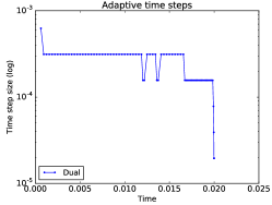
Figure 8: Adaptive time step refinement for the duality-based adaptive algorithm

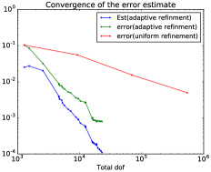
Figure 9: Convergence of the error estimate for the duality-based adaptive algorithm

7 Conclusion

In this work we carried out a comprehensive study of duality-based a posteriori error estimates for semi-linear parabolic problems, with a special focus on discretizations using the finite element method in space combined with IMEX time stepping. We introduced a decomposition of the error estimates to identify the separate error contributions due to temporal and spatial approximation. The key idea is to adapt the residual decomposition by Verfürth to our duality-based error representation and propose a specially-tailored time-discrete dual problem. The resultant error indicators quantify the spatial and temporal discretization errors and provide information to drive adaptive mesh refinement and adaptive time-step selection.

To illustrate the performance of the duality-based error estimates and the proposed adaptive algorithm, we presented numerical experiments for the heat equation and Allen–Cahn equation. We refer to [36, Section 6.3] for the application to systems. The numerical results verified the accuracy and the effectivity of the error estimate in test problems. We also observed the overall good quality of the adaptive algorithm.

The proposed methodology can be further extended to other finite difference time-stepping schemes which do not fit in our considered abstract setting, e.g. higher-order multi-stage Runge-Kutta schemes. The key challenge in any such extension is the derivation of a specially-tailored time-discrete dual problem. Our analysis indicates that these dual problems can be derived systematically by means of “backwards” summation-by-parts on the time-discrete system.

References

- [1] U. M. Ascher, Numerical methods for evolutionary differential equations, vol. 5, Siam, 2008.
- [2] L. Asner, S. Tavener, and D. Kay, Adjoint-based a posteriori error estimation for coupled time-dependent systems, SIAM Journal on Scientific Computing, 34 (2012), pp. A2394–A2419.
- [3] I. Babuška and M. Vogelius, Feedback and adaptive finite element solution of one-dimensional boundary value problems, Numerische Mathematik, 44 (1984), pp. 75–102.
- [4] R. Becker and R. Rannacher, Weighted a posteriori error control in FE methods, Citeseer, 1996.
- [5] R. Becker and R. Rannacher, An optimal control approach to a posteriori error estimation in finite element methods, Acta Numer., 10 (2001), pp. 1–102.
- [6] R. Bermejo and J. Carpio, A space–time adaptive finite element algorithm based on dual weighted residual methodology for parabolic equations, SIAM J. Sci. Comput., 31 (2009), pp. 3324–3355.
- [7] M. Besier and R. Rannacher, Goal-oriented space–time adaptivity in the finite element galerkin method for the computation of nonstationary incompressible flow, International Journal for Numerical Methods in Fluids, 70 (2012), pp. 1139–1166.
- [8] S. Boscarino, F. Filbet, and G. Russo, High order semi-implicit schemes for time dependent partial differential equations, Journal of Scientific Computing, (2016), pp. 1–27.
- [9] M. Braack, E. Burman, and N. Taschenberger, Duality based a posteriori error estimation for quasi-periodic solutions using time averages, SIAM J. Sci. Comput., 33 (2011), pp. 2199–2216.
- [10] V. Carey, D. Estep, A. Johansson, M. Larson, and S. Taverner, Blockwise adaptivity for time dependent problems based on coarse scale adjoint solutions, SIAM J. Sci. Comput., 32 (2010), pp. 2121–2145.
- [11] J. H. Chaudhry, J. Collins, and J. N. Shadid, Error estimation for multi-stage runge-kutta imex schemes, arXiv preprint arXiv:1509.08576, (2015).
- [12] J. H. Chaudhry, D. Estep, V. Ginting, J. N. Shadid, and S. Tavener, A posteriori error analysis of imex multi-step time integration methods for advection–diffusion–reaction equations, Computer Methods in Applied Mechanics and Engineering, 285 (2015), pp. 730–751.
- [13] K. Eriksson and C. Johnson, Adaptive finite element methods for parabolic problems I: A linear model problem, SIAM J. Numer. Anal., 28 (1991), pp. 43–77.
- [14] K. Eriksson and C. Johnson, Adaptive finite element methods for parabolic problems II: Optimal error estimates in and , SIAM J. Numer. Anal., 32 (1993), pp. 706–740.
- [15] K. Eriksson and C. Johnson, Adaptive finite element methods for parabolic problems IV: Nonlinear problems, SIAM J. Numer. Anal., 32 (1995), pp. 1729–1749.
- [16] K. Eriksson and C. Johnson, Adaptive finite element methods for parabolic problems V: Long-time integration, SIAM J. Numer. Anal., 32 (1995), pp. 1750–1763.
- [17] D. Eyre, Unconditionally gradient stable time marching the Cahn–Hilliard equation, in Computational and Mathematical Models of Microstructural Evolution, J. W. Bullard, L.-Q. Chen, R. K. Kalia, and A. M. Stoneham, eds., vol. 529 of Mater. Res. Soc. Symp. Proc., Warrendale, Pennsylvania, 1998, Materials Research Society, pp. 39–46.
- [18] H. Gomez and T. J. R. Hughes, Provably unconditionally stable, second-order time-accurate, mixed variational methods for phase-field models, J. Comput. Phys., 230 (2011), pp. 5310–5327.
- [19] H. Gomez and K. G. van der Zee, Computational phase-field modeling, in Encyclopedia of Computational Mechanics, Second Edition, E. Stein, R. de Borst and T.J.R. Hughes, eds., John Wiley & Sons, (2016). to appear.
- [20] D. Hilhorst, J. Kampmann, T.-N. Nguyen, and K. G. van der Zee, Formal asymptotic limit of a diffuse-interface tumor-growth model, Math. Models Methods Appl. Sci., 25 (2015), pp. 1011–1043.
- [21] J. Kim and J. Lowengrub, Phase field modeling and simulation of three-phase flows, Interfaces Free Bound., 7 (2005), pp. 435–466.
- [22] P. Krysl, E. Grinspun, and P. Schröder, Natural hierarchical refinement for finite element methods, International Journal for Numerical Methods in Engineering, 56 (2003), pp. 1109–1124.
- [23] G. Kuru, C. Verhoosel, K. Zee, and E. Brummelen, Goal-adaptive isogeometric analysis with hierarchical splines, Comput. Methods Appl. Mech. Engrg., 270 (2014), pp. 270–292.
- [24] J. T. Oden, A. Hawkins, and S. Prudhomme, General diffuse-interface theories and an approach to predictive tumor growth modeling, Math. Models Methods Appl. Sci., 20 (2010), pp. 477–517.
- [25] J. T. Oden and S. Prudhomme, Goal-oriented error estimation and adaptivity for the finite element method, Comput. Math. Appl., 41 (2001), pp. 735–756.
- [26] T. Richter and T. Wick, Variational localizations of the dual-weighted residual estimator, J. Comp. Appl. Math., 279 (2015), pp. 192–208.
- [27] M. Schmich and B. Vexler, Adaptivity with dynamic meshes for space–time finite element discretization of parabolic equations, SIAM J. Sci. Comput., 30 (2008), pp. 369–393.
- [28] J. Shen and X. Yang, Decoupled, energy stable schemes for phase-field models of two-phase incompressible flows, SIAM J. Numer. Anal., 53 (2015), pp. 279–296.
- [29] G. Şimşek, X. Wu, K. van der Zee, and E. van Brummelen, Duality-based two-level error estimation for time-dependent pdes: Application to linear and nonlinear parabolic equations, Computer Methods in Applied Mechanics and Engineering, 288 (2015), pp. 83–109.
- [30] G. Tierra and F. Guillén-González, Numerical methods for solving the Cahn–Hilliard equation and its applicability to related energy-based models, Arch. Comput. Methods Eng., 22 (2015), pp. 269–289.
- [31] E. van Brummelen, S. Zhuk, and G. van Zwieten, Worst-case multi-objective error estimation and adaptivity, Comput. Methods Appl. Mech. Engrg., 313 (2017), pp. 723–743.
- [32] K. G. van der Zee, J. T. Oden, S. Prudhomme, and A. Hawkins-Daarud, Goal-oriented error estimation for Cahn–Hilliard models of binary phase transition, Numerical Methods for Partial Differential Equations, 27 (2011), pp. 160–196.
- [33] R. Verfürth, A posteriori error estimation techniques for finite element methods, Oxford University Press, 2013.
- [34] P. Vignal, L. Dalcin, D. L. Brown, N. Collier, and V. M. Calo, An energy-stable convex splitting for the phase-field crystal equation, Comput. & Structures, 158 (2015), pp. 355–368.
- [35] S. M. Wise, C. Wang, and J. S. Lowengrub, An energy-stable and convergent finite-difference scheme for the phase field crystal equation, SIAM J. Numer. Anal., 47 (2009), pp. 2269–2288.
- [36] X. Wu, Space-Time Adaptive Methods for Phase-Field Models, PhD thesis, Technische Universiteit Eindhoven, The Netherlands, June 2017. Available at http://repository.tue.nl/866034.
- [37] X. Wu, G. J. van Zwieten, and K. G. van der Zee, Stabilized second-order convex splitting schemes for Cahn–Hilliard models with application to diffuse-interface tumor-growth models, Int. J. Numer. Meth. Biomed. Engng., 30 (2014), pp. 180–203.