Hyperscaling breakdown and Ising Spin Glasses: the Binder cumulant

Abstract

Among the Renormalization Group Theory scaling rules relating critical exponents, there are hyperscaling rules involving the dimension of the system. It is well known that in Ising models hyperscaling breaks down above the upper critical dimension. It was shown by M. Schwartz [Europhys. Lett. 15, 777 (1991)] that the standard Josephson hyperscaling rule can also break down in Ising systems with quenched random interactions. A related Renormalization Group Theory hyperscaling rule links the critical exponents for the normalized Binder cumulant and the correlation length in the thermodynamic limit. An appropriate scaling approach for analyzing measurements from criticality to infinite temperature is first outlined. Numerical data on the scaling of the normalized correlation length and the normalized Binder cumulant are shown for the canonical Ising ferromagnet model in dimension three where hyperscaling holds, for the Ising ferromagnet in dimension five (so above the upper critical dimension) where hyperscaling breaks down, and then for Ising spin glass models in dimension three where the quenched interactions are random. For the Ising spin glasses there is a breakdown of the normalized Binder cumulant hyperscaling relation in the thermodynamic limit regime, with a return to size independent Binder cumulant values in the finite-size scaling regime around the critical region.

I Introduction

The consequences of the Renormalization Group Theory (RGT) approach have been studied in exquisite detail in numerous regular physical models, typified by the canonical near-neighbor interaction ferromagnetic Ising models. It has been tacitly assumed that Edwards-Anderson Ising Spin Glasses (ISGs), where the quenched interactions are random, follow the same basic scaling and Universality rules as the Ising models.

The Binder cumulant binder:81 is an important observable which has been almost exclusively exploited numerically for its scaling properties as a dimensionless observable very close to criticality in the finite-size scaling (FSS) regime $L\ll\xi(\beta)$, where $L$ is the sample size and $\xi(\beta)$ is the second-moment correlation length at inverse temperature $\beta$. Here we will consider its scaling properties over the whole temperature region, in particular in the Thermodynamic limit (ThL) regime $L\gg\xi(\beta)$ where the properties of a finite-size sample normalized appropriately are independent of $L$ and so are the same as those of the infinite-size model.

We will explain in detail the overall scaling analysis procedure, based on Ref. wegner:72 ; privman:91 ; campbell:06 , which we use in both the cases of standard Ising models and of ISGs.

II Scaling

In numerical simulation analyses the conventional RGT based approach consists in using as the thermal scaling variable the reduced temperature $t=(T-T_{c})/T_{c}$, together with the principal observables $\chi(t,L)$ the susceptibility, $\xi(t,L)$ the second moment correlation length, and $g(t,L)$ the Binder cumulant. (For finite-size simulation data the standard finite-$L$ definition for the second moment correlation length $\xi(\beta,L)$ through the Fourier transformation of the correlation function is used, see for instance Ref. hasenbusch:08 Eq. $14$). The conventional approach is tailored to the critical region; however at high temperatures $t$ diverges and $\xi(t,L)$ tends to zero, so it is not possible to analyse the entire paramagnetic regime without introducing diverging correction terms. For the Ising systems this problem can be eliminated by using the inverse temperature $\beta=1/T$, a practice which pre-dates RGT.

The thermal scaling variable $t$ is also widely used in analyses of simulation data in ISGs. As the relevant interaction strength in ISGs is $[\langle J_{ij}^{2}\rangle]$, the symmetric interaction distribution ISG thermal scaling variable should logically depend on the square of the temperature; this basic point was made some thirty years ago singh:86 but has generally been ignored.

As a basis for a rational scaling approach which englobes the entire paramagnetic region so including both the finite-size scaling regime (FSS, $L\ll\xi(\beta,\infty)$) and the thermodynamic-limit regime (ThL, $L\gg\xi(\beta,\infty)$), we start from the Wegner ThL scaling expression for the Ising susceptibility wegner:72

$$\chi(\tau)=C_{\chi}\tau^{-\gamma}\left(1+a_{\chi}\tau^{\theta}+b_{\chi}\tau+\cdots\right)$$ (1)

where $\tau=1-\beta/\beta_{c}$ with $\beta$ the inverse temperature. (The Wegner expression is often mis-quoted with $t$ replacing $\tau$). The terms inside $(..)$ are scaling corrections, with $\theta$ the leading correction exponent which is universal for all observables. As $\tau$ and $\chi(\tau)$ both tend to $1$ at infinite temperature, the whole paramagnetic region can be covered without divergencies, to good precision when a small number of well-behaved correction terms are included. (To obtain infinite precision an infinite number of correction terms would be needed, just as in standard FSS analyses perfect precision in principle requires a series of corrections to infinite $L$). In ISG models where the interaction distributions are symmetric about zero, an appropriate thermal scaling variable to be used with the same Wegner expression is $\tau=1-(\beta/\beta_{c})^{2}$, Refs. singh:86 ; klein:91 ; daboul:04 ; campbell:06 . In the ThL regime $L\gg\xi(\beta)$ the properties of a finite-size sample, if normalized correctly, are independent of $L$ and so are the same as those of the infinite-size model. A standard rule of thumb for the approximate onset of the ThL regime is $L>7\xi(\beta,L)$ and the ThL regime can be easily identified in simulation data. An important virtue of this approach is that the ThL numerical data can be readily dovetailed into High Temperature Series Expansion (HTSE) values calculated from sums of exact series terms (limited in practice to a finite number of terms). No such link can be readily made when the conventional FSS thermal scaling variable $t$ is used.

To apply the Wegner formalism to observables $Q$ other than $\chi$, we introduce the rule that these observables should be normalized in such a way that the infinite-temperature limit $Q(\tau=1)\equiv 1$, without the critical limit being modified. For the susceptibility with the standard definition no normalization is required as this condition is automatically fulfilled, with a temperature-dependent effective exponent $\gamma(\tau)=\partial\ln\chi(\tau,L)/\partial\ln\tau$ in Ising models and in ISGs with the appropriate $\tau$. Then

$$\gamma(\tau)=\gamma-\frac{a_{\chi}\theta\tau^{\theta}+b_{\chi}\tau}{1+a_{\chi}\tau^{\theta}+b_{\chi}\tau}$$ (2)

to second order in the corrections lundow:15 .

In Ref. campbell:06 the normalized second-moment correlation length was introduced : $\xi(\tau,L)/\beta^{1/2}$ in Ising models and $\xi(\tau,L)/\beta$ in ISG models. From exact and general HTSE infinite-temperature limits, this normalized correlation length tends to exactly $1$ at infinite temperature butera:02 ; daboul:04 . The temperature-dependent effective exponent is $\nu(\tau)=\partial\ln[\xi(\tau,L)/\beta^{1/2}]/\partial\ln\tau$ in Ising models and $\nu(\tau)=\partial\ln[\xi(\tau,L)/\beta]/\partial\ln\tau$ in ISG models. A Wegner-like relation is

$$\xi(\tau)/\beta^{1/2}=C_{\xi}\tau^{-\nu}\left(1+a_{\xi}\tau^{\theta}+b_{\xi}\tau+\cdots\right)$$ (3)

so

$$\nu(\tau)=\nu-\frac{a_{\xi}\theta\tau^{\theta}+b_{\xi}\tau}{1+a_{\xi}\tau^{\theta}+b_{\xi}\tau}$$ (4)

The critical limiting ThL exponent $\nu$ is unaltered by this normalization (models with zero critical temperatures are a special case). The normalized correlation length can be accurately expressed over the entire paramagnetic region with a limited number of generally weak correction terms. The temperature-dependent effective exponents $\gamma(\tau)$ and $\nu(\tau)$ are well-behaved over the whole paramagnetic regime with the exact infinite-temperature hypercubic lattice limits for Ising models of $\gamma(1)=2D\beta_{c}$ and $\nu(1)=D\beta_{c}$, and for the ISG models $\gamma(1)=2D\beta_{c}^{2}$ and $\nu(1)=(D-K/3)\beta_{c}^{2}$ where $K$ is the kurtosis of the interaction distribution and $D$ is the dimension. The normalized Binder cumulant scaling is discussed below.

III Hyperscaling

Among the standard rules linking critical exponents are the hyperscaling relations widom:65 ; kadanoff:66 ; josephson:66 . A textbook definition of hyperscaling is : ”Identities obtained from the generalised homogeneity assumption involve the space dimension D, and are known as hyperscaling relations.” simons:97 . The most familiar form of the hyperscaling relation is $\alpha=2-D\nu$ which through the Essam-Fisher relation $\alpha+D\nu-2\Delta=2$ can be re-written $2\Delta=\gamma+D\nu$. $\Delta$ is the Gap exponent, defined butera:02 through the critical behavior of the higher field derivatives of the free energy, $\gamma_{k}=\gamma+(k-2)\Delta$ ; $\Delta=\gamma+\beta$ .

This form of the hyperscaling relation has practical consequences for the scaling of the normalized Binder cumulant. Hyperscaling is well established in standard models, such as the Ising models in dimensions less than the upper critical dimension, see Section IV. The specific case of breakdown of hyperscaling for the Ising model in dimension $5$, above the upper critical dimension, is discussed in Section V.

In Ising ferromagnets, in the thermodynamic limit (infinite size or $L\gg\xi(\tau)$) regime the susceptibility $\chi(\beta)$ scales with the critical exponent $\gamma$, and assuming hyperscaling the critical exponent for the second field derivative of the susceptibility $\chi_{4}(\beta)$ (also called the non-linear susceptibility) is  butera:02

$$\gamma_{4}=\gamma+2\Delta_{\mathrm{gap}}=D\nu+2\gamma$$ (5)

Note that $\chi_{4}$ in a hypercubic lattice is directly related to the Binder cumulant through

$$2g(\beta,L)=\frac{-\chi_{4}}{L^{D}\chi^{2}}=\frac{3\langle m^{2}\rangle^{2}-\langle m^{4}\rangle}{\langle m^{2}\rangle^{2}}$$ (6)

see Eq. (10.2) of Ref. privman:91 . Thus in the ThL regime the normalized Binder cumulant $L^{D}g(\beta,L)$ (or alternatively $-\chi_{4}(\beta)/(2\chi(\beta)^{2})$) scales with the critical exponent $(\nu D+2\gamma)-2\gamma=\nu D$, together with correction terms as for any such observable, because of the RGT scaling and hyperscaling widom:65 ; josephson:66 relationships between exponents. Here $\nu$ and $\gamma$ are the standard critical exponents for the correlation length and the susceptibility.

It can be noted that in any $S=1/2$ Ising system the infinite-temperature (i.e. independent spins) limit for the Binder cumulant is $g(0,N)\equiv 1/N$, where N is the number of spins; as $N=L^{D}$ for a hypercubic lattice, at infinite temperature $L^{D}g(\tau,L)\equiv 1$. Thus the Ising normalized Binder cumulant obeys the high temperature limit rule for normalized observables introduced above.

Two forms of the hyperscaling relation have been quoted above; the first is well known and concerns the specific heat exponent $\alpha$. Many years ago this first hyperscaling relation was predicted by Schwartz to break down in quenched random systems schwartz:91 . The breakdown of this hyperscaling relation in the Random Field Ising model (RFI) has been extensively studied gofman:93 ; vink:10 ; fytas:13 . Ising spin glasses (ISGs) are also systems with quenched randomness in which hyperscaling might be expected to break down by a generalisation of Schwartz’s argument. The exponent $\alpha$ in ISGs is always strongly negative and so is very hard to measure directly; we will explore only the second form of the hyperscaling relation which is less well known. We are aware of no tests of this hyperscaling relation in ISGs.

We observe that in ISGs the ThL susceptibility $\chi(\tau)$ and the normalized second moment correlation length $\xi(\tau)T$ follow the Wegner scaling rules with only weak corrections over the entire temperature range from criticality to infinity as has already been shown, e.g. Ref. campbell:06 ; lundow:15a . However, in ISGs for the normalized Binder cumulant $L^{D}g(\tau,L)$ we indeed find very strong deviations from the behaviour expected if hyperscaling held. Because of difficulties inherent to ISG simulations, the ThL temperature range attainable in the present measurements is restricted so these deviations cannot be fully characterized, though it seems unlikely that a huge and unspecified “correction term” should just appear by accident.

IV Privman-Fisher scaling and Extended scaling

Up to now we have been considering only data in the ThL. Writing for an Ising ferromagnet model with the normalized correlation length $\xi(\tau,\infty)\sim\beta^{1/2}\tau^{-\nu}$ in the ThL and for an observable $Q(\tau,L)$ where $Q(\tau,\infty)\sim\tau^{-q\nu}$ at criticality, ignoring corrections to scaling the Privman-Fisher finite-size rule privman:91 can be written

$$\frac{Q(\tau,L)}{Q(\tau,\infty)}=F[L/\xi(\tau,\infty)]=F[LT^{1/2}\tau^{\nu}]$$ (7)

or

$$Q(\tau,L)=F[LT^{1/2}\tau^{\nu}]/\tau^{q\nu}$$ (8)

or

$$\frac{Q(\tau,L)}{(LT^{1/2})^{q}}=\frac{F[LT^{1/2}\tau^{\nu}]}{\tau^{q\nu}(LT^{1/2})^{q}}=\frac{F[LT^{1/2}\tau^{\nu}]}{(\tau^{\nu}LT^{1/2})^{q}}$$ (9)

or finally

$$\frac{Q(\tau,L)}{(LT^{1/2})^{q}}=F^{*}[(LT^{1/2})^{1/\nu}\tau]$$ (10)

which is the ”extended scaling” form of Ref. campbell:06 . For an ISG, $T^{1/2}$ is replaced throughout by $T$. If Wegner corrections to scaling factors have been measured from ThL data, these can be readily introduced into either the Privman-Fisher expression or the extended scaling expression. The two scalings are broadly equivalent in that data for all sizes are included in the scaling plots. Depending on the circumstances one or other scaling can be easier to ”read”.

For specific normalized observables,

• when $Q$ is the normalized correlation length $\xi(\tau,L)T^{1/2}$, with $q=1$,

  $$Q(\tau,L)/(LT^{1/2})^{q}=\xi(\tau,L)/L$$ (11)

  so the scaling rule is campbell:06

  $$\xi(\tau,L)/L=F^{*}[(LT^{1/2})^{1/\nu}\tau]$$ (12)

• when $Q$ is $\chi(\tau,L)$, with $q=2-\eta$, the scaling rule is campbell:06

  $$\chi(\tau,L)/(LT^{(}1/2))^{2-\eta}=F^{*}[(LT^{1/2})^{1/\nu}\tau]$$ (13)

• for an Ising model when $Q$ is the normalized Binder cumulant $L^{D}g(\tau,L)$, with $q=D$ if hyperscaling holds,

  $$\frac{Q(\tau,L)}{(LT^{1/2})^{q}}=\frac{L^{D}g(\tau,L)}{(LT^{1/2})^{D}}=\frac{g(\tau,L)}{T^{D/2}}$$ (14)

  so the scaling rule is

  $$g(\tau,L)/T^{D/2}=F^{*}[(LT)^{1/\nu}\tau]$$ (15)

  (This expression was not cited in Ref. campbell:06 ). For the particular case of the $D=5$ Ising model, $\nu=1/2,\eta=0$ and the standard hyperscaling rules do not hold. The modified scaling rules are discussed below in Section VI.

Again, for an ISG $T^{1/2}$ is replaced throughout by $T$. Finally, as the scaling rules for the correlation length and for the Binder cumulant have the same $x$-axis $(LT^{1/2})^{1/\nu}\tau$, if hyperscaling holds a further scaling plot is given by $y(T,L)=g(T,L)/T^{D/2}$ against $x(T,L)=\xi(T,L)/L$ (or for an ISG $y(T,L)=g(T,L)/T^{D}$ against $x(T,L)=\xi(T,L)/L$). This is a particularly remarkable format as both $x(T,L)$ and $y(T,L)$ represent purely measured data sets; no inputs concerning the values of $T_{c}$ or of the critical exponents are required for the scaling. This type of plot can represent a stringent test of hyperscaling.

V The 3D Ising model

We will first consider the canonical cubic lattice Ising model in dimension $3$, in order to exhibit a case where hyperscaling is well established. Critical temperature $\beta_{c}$ and the critical exponents are known to very high precision in this model simmons:15 . Simulation data were mainly taken from Ref. haggkvist:07 . See Ref. campbell:11 for detailed Privman-Fisher and extended scaling analyses of $\chi(\tau,L)$ in this model including the correction terms. Scalings for the correlation length $\xi(\tau,L)$ are shown in Figs. 1 and 2.

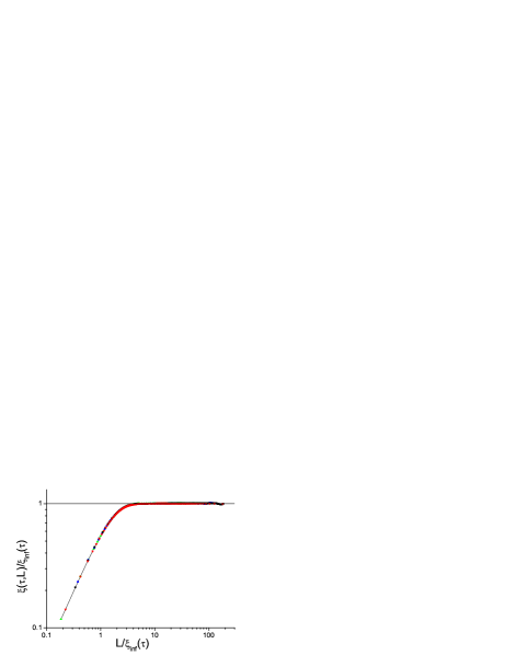
Figure 1: (Color on line) Dimension 3 Ising model Privman-Fisher finite-size scaling plot for the correlation length. Sample sizes $L=32$ (black squares), $L=24$ (blue circles), $L=16$ (green triangles), $L=8$ (red inverted triangles). $\xi_{\infty}(\tau)=1.074\tau^{-0.630}\beta^{1/2}(1-0.12\tau^{0.5}+0.05\tau)$

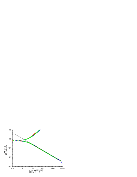
Figure 2: (Color on line) Dimension 3 Ising model extended scaling plot for the correlation length. Sample sizes as indicated in Fig. 1. Upper branch $\beta>\beta_{c}$, lower branch $\beta<\beta_{c}$. The black straight line has slope $-\nu$.

The ThL susceptibility and normalized correlation length corrections are relatively small for both observables campbell:11 and the extended scaling expressions with only two leading Wegner correction terms give rather accurate fits to the ThL simulation and HTSE data over the whole paramagnetic temperature range. (Scaling with $\xi(t,L)$ rather than with $\xi(\tau,L)/\beta^{1/2}$ leads to a high temperature ”cross-over” behavior in Ising ferromagnets luijten:97 which is an artefact lundow:11 ).

For the Binder cumulant in the $3$D Ising model, ThL simulation and HTSE data (evaluated from the tabulated series in Ref. butera:02a ) can be fitted satisfactorily by

$$L^{D}g(\tau,L)=1.57\tau^{-1.89}\left(1-0.294\tau-0.069\tau^{2.85}\right)$$ (16)

where the critical exponent is equal to $D\nu=3\cdot 0.63$ as expected from hyperscaling, see Figs. 3 and 4. The amplitude of the expected leading confluent correction term proportional to $\tau^{0.523}$ turns out to be negligible for the Binder cumulant in the 3D Ising universality class lundow ; the next effective correction terms proportional to $\tau$ and to $\tau^{\theta_{\mathrm{eff}}}\sim\tau^{2.85}$ dominate the corrections

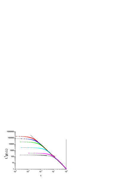
Figure 3: (Color on line) Dimension 3 Ising model normalized Binder cumulant $L^{3}g(\tau,L)$ as a function of $\tau$ for $L=64$, $48$, $32$, $16$, $8$ (top to bottom). The open points are the sum of the first 8 HTSE values evaluated from Ref. butera:02a . Exponent $1.89=3\nu$; fit $(L^{3}g(\tau,L))_{\infty}=1.57\tau^{-1.89}(1-0.294\tau-0.069\tau^{2.85})$. Slope $-1.89$ black curve.

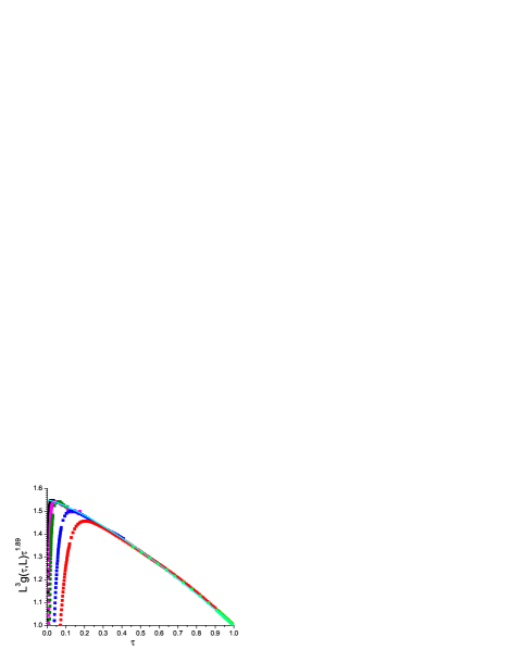
Figure 4: (Color on line) Dimension 3 Ising model normalized Binder cumulant $L^{3}g(\tau,L)\tau^{1.89}$ correction factor as a function of $\tau$ for $L=48$, $32$, $24$, $12$, $8$ (top to bottom). Fit of $L^{3}g(\tau,L)\tau^{1.89}=1.55(1-0.294\tau-0.069\tau^{2.85})$ cyan curve.

Privman-Fisher and extended scaling format plots of the normalized Binder cumulant $L^{3}g(\tau,L)$ for all measured $L$ and $\tau$ are shown in Figs. 5 and 6. The overall scalings hold well for all temperatures and for all sizes from infinity down to criticality (and even somewhat beyond as the extended scaling plots show), as to be expected for a model where hyperscaling holds.

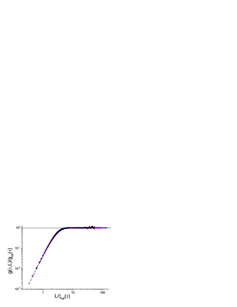
Figure 5: (Color on line) Dimension 3 Ising model Privman-Fisher plot of the Binder cumulant. Point coding as in Fig. 4; $\nu=0.63$. The $g_{\infty}(\tau)$ as in caption of Fig. 3 and $\xi_{\infty}(\tau)$ as in caption of Fig. 1.

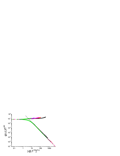
Figure 6: (Color on line) Dimension 3 Ising model extended scaling plot of the Binder cumulant. Point coding as in Fig. 4. The straight line has slope $-3\nu$, with $\nu=0.63$.

As a direct test of the Binder cumulant hyperscaling we can make up a pure data-against-data plot of $y(T,L)=g(T,L)/T^{3/2}$ against $x(T,L)=\xi(T,L)/L$, see Fig. 7, again assuming hyperscaling so $q=3$. The overall scaling is good over the whole temperature range shown. (The empirical $g(T,L)$ against $\xi(T,L)$ form of scaling of the same data, which has been suggested for instance in Ref. jorg:06 , appears satisfactory when presented as a linear-linear plot but is unsatisfactory when presented as a log-log plot covering the entire temperature range).

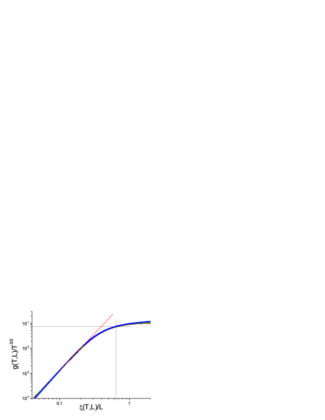
Figure 7: (Color on line) Dimension 3 Ising model normalized scaling plot of Binder cumulant against correlation length with no input parameters. Sizes shown are $L=32$ (black squares), $L=24$ (red circles), $L=12$ (green triangles), $L=8$ (blue inverted triangles). Dashed lines indicate criticality.

VI The 5D Ising model

The upper critical dimension of standard Ising models is $D_{\mathrm{ucd}}=4$. For higher dimensions critical exponents are mean field (MF) and independent of $D$ : $\alpha=0$, $\nu=1/2$, $\gamma=1$, $\eta=0$, $\omega=1$. It is well known that the standard hyperscaling relation $\alpha=2-D\nu$ cannot hold above $D=4$ as this relation is incompatible with the MF exponents. A general rule for the FSS correlation length above $D_{\mathrm{ucd}}$ which holds both for periodic boundary conditions and for free boundary conditions, is $\xi(\tau,L)\sim L^{\hbox{\coppa}}$ with $\hbox{\coppa}=D/D_{\mathrm{ucd}}$ berche:12 . Indeed it has been shown that above $D=4$ at criticality the effective finite-size correlation length $\xi(\tau_{c},L)$ scales with $L^{D/4}=L^{\hbox{\coppa}}=L^{D/D_{\mathrm{ucd}}}$ rather than with $L$ while the critical Binder cumulant $g(\tau_{c},L)$ remains independent of $L$ (to within corrections to scaling) jones:11 ; berche:12 . In the Privman-Fisher and extended scaling plots shown in Figs. 8, 10 and 11 $L^{D/D_{\mathrm{ucd}}}$ replaces $L$ everywhere, showing that the FSS rule for $D$ above $D_{\mathrm{ucd}}$ is valid in the whole paramagnetic temperature range.

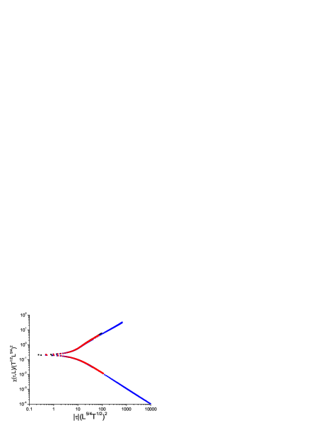
Figure 8: (Color on line) Dimension 5 Ising model. Susceptibility extended scaling. Sizes shown are $L=24$ (black squares), $L=16$ (red circles), $L=8$ (blue triangles). Upper branch $\beta>\beta_{c}$.

The MF value of the gap exponent is $\Delta=3/2$ butera:12 , so the second standard hyperscaling rule $2\Delta=D\nu+\gamma$ must also be violated above $D=4$. From the same reasoning as above, it follows that this hyperscaling breakdown leads to a MF ThL exponent for the normalized Binder cumulant which is $2$ rather than $D\nu=D/2$, so in the ThL $L^{D}g(\tau,L)\sim\tau^{-2}$. Simulation data in dimension $5$ for $L^{5}g(\tau,L)$ as a function of $\tau$ are shown in Fig. 9 where it can be seen that in the entire ThL regime from infinite temperature to criticality this rule indeed holds with a critical exponent $2$ and a weak correction to scaling. The critical amplitudes for $\chi_{4}$ and $\chi$ are $\sim 1.40$ butera:12a and $\sim 1.29$ berche:08 ; butera:12a respectively, and the leading thermal correction exponent is $\theta=\omega\nu=1/2$, so including the leading correction term the ThL scaling is $L^{D}g(\tau,L)=0.80\tau^{-2}(1+0.176\tau^{1/2})$ (It should be noticed that for $D=5$ the form of the normalization of the Binder cumulant remains $L^{5}g(\tau,L)$, and does not become $L^{25/4}g(\tau,L)$ because $L^{5}$ is just the number of spins).

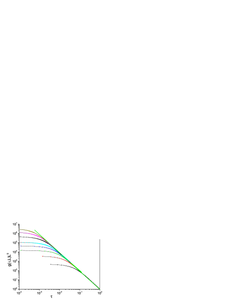
Figure 9: (Color on line) Dimension 5 Ising model. Normalized Binder cumulant against $\tau$ for $L=24$, $20$, $16$, $12$, $10$, $8$, $6$, $4$ (top to bottom). Fit : full green curve.

This behavior would not have been recognized easily if the conventional reduced temperature $t=1-T/T_{c}$ had been used as the scaling parameter. The Privman-Fisher Binder cumulant scaling (without correction terms) with $\nu=1/2$, $q=4$, $L^{5}g(\tau,L)\sim\tau^{-2}$, $\xi(\tau,\infty)=\beta^{1/2}\tau^{-1/2}$ and $L^{5}g(\tau,L)/L^{5}g(\tau,\infty)=F[L^{5/4}/\xi(\tau,\infty)]$ becomes $g(\tau,L)/T^{2}=F^{*}[L^{5/2}\tau T]$ which is consistent with an $L$ independent $g(0,L)=F^{*}(0)$ at criticality ($\tau=0$, $T=T_{c}$) to within correction terms.

Correction terms can be included in the Privman-Fisher scaling. We have no simulation or HTSE data for the correlation length in dimension $5$. However, we assume that the ThL correlation length behaves as $\xi(\tau,\infty)=C\beta^{1/2}\tau^{-1/2}[1-(1-1/C)\tau^{1/2}]$ with a weak leading order scaling correction (as observed for Ising models in dimensions $2$ and $3$ campbell:08 ; campbell:11 ). The dimension $5$ modified Privman-Fisher scaling rule for an observable $Q$ is

$$\frac{Q(\tau,L)}{Q(\tau,\infty)}=F[L^{5/4}/\xi(\tau,\infty)]$$

$$=F[L^{5/4}/(C\beta^{1/2}\tau^{-1/2}(1-(1-1/C)\tau^{1/2}))]$$ (17)

Scaled data for for the normalized Binder cumulant $Q=L^{5}g(\tau,L)$ and $q_{g}=2/\nu=4$, are shown in Fig. 10 and Fig. 11. With the correlation length critical amplitude chosen as $C=0.75$ to optimize the $\chi$ scaling, both scalings are excellent. This validates the correlation length normalization form $\xi(\tau,\infty)/\beta^{1/2}$ in 5D, and the replacement of $L$ by $L^{5/4}$ in the Privman-Fisher correlation length scaling rule not only in a narrow critical region but in the entire paramagnetic regime. The plots cover data for all sizes from infinite temperature to criticality (the left hand $\tau=0$ limit in Fig. 10) and even to well beyond criticality (the upper branch in Fig. 11).

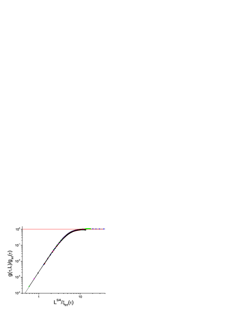
Figure 10: (Color on line) Dimension 5 Ising model Binder cumulant Privman-Fisher scaling for $L=16$ (black squares), $L=10$ (pink circles), $L=8$ (green triangles), $L=6$ (red inverted triangles), $L=4$ (blue diamonds).

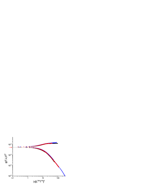
Figure 11: (Color on line) Dimension 5 Ising model extended scaling of the Binder cumulant for $L=24$ (black squares), $L=12$ (red triangles), $L=6$ (blue circles). Upper branch $\beta>\beta_{c}$. Arrow : critical value from Ref. jones:11 .

In the FSS limit close to criticality this scaling implies that $g(\tau_{c},L)$ is independent of $L$ (to within corrections to scaling), which is consistent with the data of Ref. jones:11 . The preservation of the rule of size independence for the dimensionless Binder cumulant at criticality results from the combined effects of the two hyperscaling breakdowns. The susceptibility $\chi(\tau,L)$ finite-size scaling becomes $\chi(\tau_{c},L)\sim L^{5/2}$ at criticality. If data were available, the overall Privman-Fisher correlation length scaling rule would be

$$\xi(\tau,L)/L^{5/4}=F[L^{5/4}/(\beta^{1/2}\tau^{-1/2})]$$ (18)

so with $\xi(\tau_{c},L)/L^{5/4}$ independent of $L$ at criticality to within the correction term, as observed in Ref. jones:11 . An analysis of Ising data in dimension $6$ shows that they follow just the same rules as in dimension $5$ mutatis mutandis (so with $\hbox{\coppa}=3/2$), again over the entire paramagnetic regime. Thus the ThL $L^{6}g(\tau,L)$ has critical exponent $2$ as in 5D, and the Privman Fisher scaling rules all work with $x$-axis $L^{6/4}/\xi(\tau,\infty)$ for all temperatures.

VII Ising spin glasses

Now we turn to ISGs. The standard ISG Hamiltonian is $\mathcal{H}=-\sum_{ij}J_{ij}S_{i}S_{j}$ with the near neighbor symmetric random distributions normalized to $\langle J_{ij}^{2}\rangle=1$. The normalized inverse temperature is $\beta=(\langle J_{ij}^{2}\rangle/T^{2})^{1/2}$. The Ising spins live on simple hyper-cubic lattices with periodic boundary conditions. For the bimodal models $J_{ij}=\pm 1$ at random. The spin overlap parameter is defined as usual by

$$q=\frac{1}{L^{D}}\sum_{i}S^{A}_{i}S^{B}_{i}$$ (19)

where $A$ and $B$ indicate two copies of the same system. Klein et al. klein:91 quote exactly the same hyperscaling relation Eq. (5) for $\chi_{4}$ in the ISGs as in the Ising ferromagnets (with the spin overlap moments $\langle q^{2}\rangle$ and $\langle q^{4}\rangle$ replacing the magnetization moments $\langle m^{2}\rangle$ and $\langle m^{4}\rangle$), so the RGT hyperscaling prediction for the ISG Binder cumulant critical exponent is again $\gamma_{4}-2\gamma=D\nu$. Because the interaction parameter in the ISGs is $\langle J_{ij}^{2}\rangle$ the appropriate ISG temperature scaling variable is $\tau=1-(\beta/\beta_{c})^{2}$ daboul:04 ; campbell:06 and the appropriate normalized correlation length is $\xi(\tau,L)/\beta$ campbell:06 .

Some of the simulation data in the ISGs are the same as those in Refs. lundow:15 ; lundow:15a where the simulation techniques have already been described in detail. Means were taken on at least $8192$ samples for each $L$ with of the order of $40$ different temperatures. The maximum size studied was $L=32$. Particular attention was paid to achieving full equilibration. For the $3$D bimodal model comparisons with tabulated data generously provided by H. Katzgraber and by K. Hukushima from independent simulations, and from raw data tabulations related to Ref. hasenbusch:08 helpfully published on line by Hasenbusch, Pelissetto and Vicari, confirm equilibration. Unfortunately the maximum sizes $L$ for simulations in ISGs have been limited in practice by the available computational ressources and we know of no published measurements to $L$ greater than $40$ in $D=3$. For the 3D bimodal ISG extended scaling plots for $\chi(\tau,L)$ and $\xi(\tau,L)/\beta$ were shown in Ref. campbell:06 with fit values for the critical parameters close to those estimated later from FSS analyses katzgraber:06 ; hasenbusch:08 ; baity:13 . Assuming $\beta_{c}=0.9075$ (from Ref. baity:13 , which is consistent with the estimates of Refs. katzgraber:06 and hasenbusch:08 to within the quoted errors) we have made plots of the temperature dependent effective exponents $\gamma(\tau,L)$ and $\nu(\tau,L)$ lundow .

Extrapolating to criticality, the estimations for the critical exponents are $\gamma=6.15(10)$ in agreement with Ref. baity:13 , and $\nu=2.45(10)$, in good agreement with the estimate of Ref. hasenbusch:08 (but significantly lower than the estimate of Ref. baity:13 ). With these values in hand we fit the ThL susceptibility and correlation length data with leading effective corrections lundow

$$\chi(\tau) = 1.28\tau^{-6.15}\left(1-0.62\tau^{2.45}+0.405\tau^{7}\right)$$ (20)

$$\xi(\tau) = 1.15\tau^{2.45}\beta\left(1-0.24\tau^{2.45}+0.11\tau^{7}\right)$$ (21)

It can be noted that when the $\beta$ normalization factor is included, the correction terms for the normalized $\xi(\tau)/\beta$ are weak over the entire temperature range, as already observed in campbell:06 . (In the dimension 3 bimodal ISG for both observables it is essential to introduce two correction terms for a satisfactory fit over the whole paramagnetic temperature range. This implies that in principle two corresponding correction terms should also be included in FSS analyses). Standard Privman-Fisher scaling for $\chi(\tau,L)$ and for the normalized correlation length $\xi(\tau,L)/\beta$ with the correction terms are shown in Figs. 12 and 13, now including all the data and not just the ThL data. The overall scaling for all paramagnetic temperatures and all sizes is excellent which in particular is consistent with the extrapolations to criticality being valid.

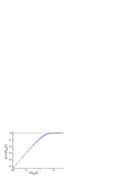
Figure 12: (Color on line) Dimension 3 bimodal interaction ISG Privman-Fisher susceptibility scaling for $L=32$ (open squares), $L=20$ (black squares), $L=10$ (red circles), $L=6$ (blue triangles). For $\chi_{\infty}(\tau),\xi_{\infty}(\tau)$, see text.

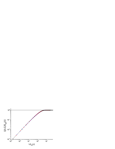
Figure 13: (Color on line) Dimension 3 bimodal interaction ISG Privman-Fisher correlation length scaling for $L=32$ (open squares), $L=20$ (black squares), $L=10$ (red circles), $L=6$ (blue triangles). For $\xi_{\infty}(\tau)$, see text.

In Fig. 14 the normalized Binder cumulant $L^{3}g(\tau,L)$ against $\tau$ data are shown. Sizes $L$ are limited by the rapidly increasing numbers of spins and by equilibration difficulties; the lowest value of $\tau$ where the ThL condition still holds is only about $0.5$. Down to this lowest accessible ThL value of $\tau$, the ThL data can be fitted approximately by $L^{3}g(\tau,L)\sim\tau^{-10.5}$ with a correction term, so an effective exponent much larger than the hyperscaling value $3\nu=7.35$. If data for much higher $L$ (and so to lower $\tau$-values still within the ThL regime) were available there seems no a priori reason to expect this behavior with a large effective exponent to change.

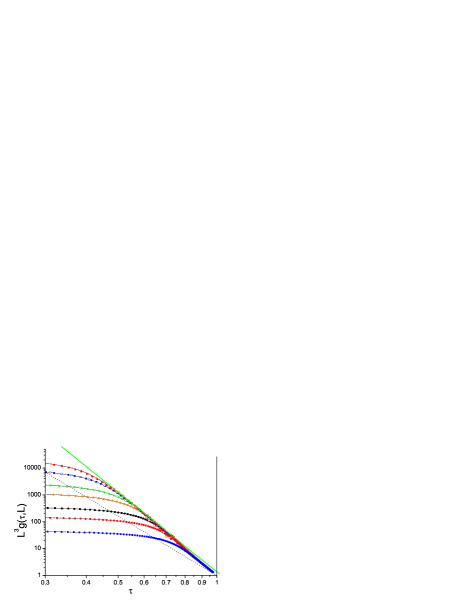
Figure 14: (Color on line) Dimension 3 bimodal interaction ISG normalized Binder cumulant against $\tau$ for $L=32$, $24$, $16$, $12$, $8$, $6$, $4$ (top to bottom). Dashed line : slope $7.35=3\nu$, full green line slope $10.3$.

In Figs. 15 and 16 the Privman-Fisher scaling curves are shown for the same 3D bimodal normalized Binder cumulant data assuming hyperscaling, i.e. with a critical exponent equal to $7.35$. In the ThL regime (on the right) the scaled curves have peaks increasing dramatically in size, and moving to the left regularly with increasing $L$. The peaks reach values of the order of $10$ for the sizes covered by the present measurements, far from remaining near $y(x)\sim 1$ as would be expected if the hyperscaling rule was obeyed and as is observed above for $\chi(\tau,L)$ and $\xi(\tau,L)/\beta$ Privman-Fisher plots where hyperscaling is not involved. (While scaling analyses of the $\chi(\tau,L)$ and $\xi(\tau,L)T$ data for the 3D bimodal and Gaussian ISGs show typical critical amplitudes $C\sim 1.10$ associated with weak correction terms lundow , attempts to fit the $L^{3}g(\tau,L)$ data with critical exponent $D\nu$ plus corrections lead to huge critical amplitudes $C\sim 25$, and exotic correction terms. This interpretation appears unphysical). However, on leaving the ThL regime as temperatures tend towards criticality, the hyperscaling behavior with curves for all $L$ overlapping is gradually recovered in the FSS regime.

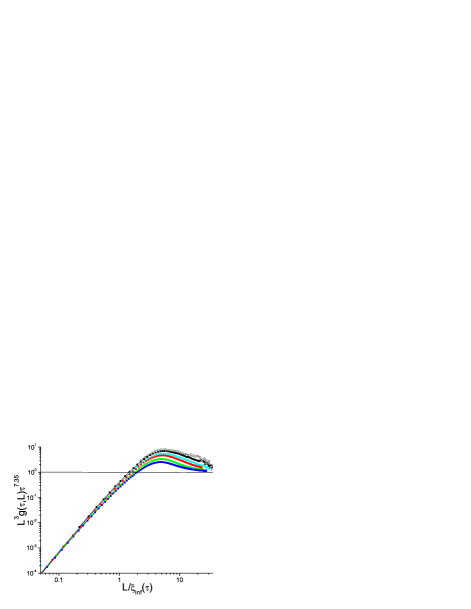
Figure 15: (Color on line) Dimension 3 bimodal interaction ISG normalized Binder cumulant Privman-Fisher plot assuming hyperscaling. Sizes shown are $L=32$, $24$, $16$, $12$, $8$, $6$ (top to bottom).

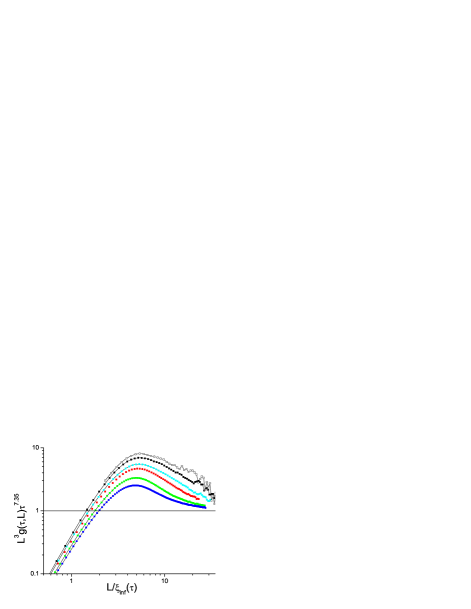
Figure 16: (Color on line) Dimension 3 bimodal interaction ISG normalized Binder cumulant Privman-Fisher plot assuming hyperscaling. Zoom of Fig. 15.

An extended scaling plot assuming hyperscaling, $g(\tau,L)/T^{3}$ against $\xi(\tau,L)/L$ in Fig. 17 should show curves for all $L$ overlapping as for the 3D Ising model, see Fig. 7. Again there are strong deviations in the ThL regime on the left (and also for $\beta>\beta_{c}$ on the right) with hyperscaling behavior restored at criticality indicated by the dashed lines.

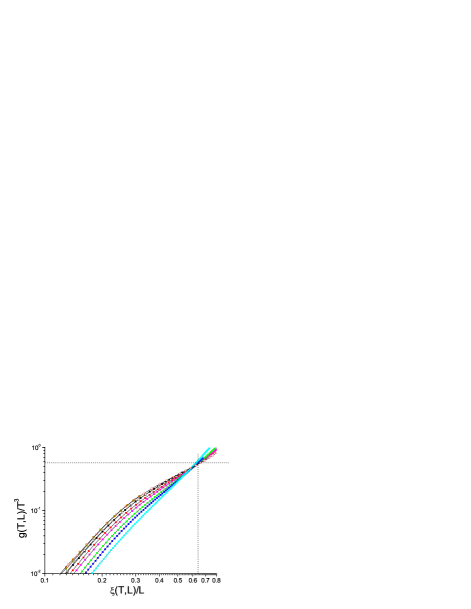
Figure 17: (Color on line) Dimension 3 bimodal interaction ISG. Normalized Binder cumulant scaling of $g(\tau,L)/T^{3}$ against $\xi(\tau,L)/L$ assuming hyperscaling

The most recent estimates of the dimension 3 Gaussian interaction ISG critical parameters katzgraber:06 are $\beta_{c}=1.05(1)$, $\nu=2.44(9)$, and $\eta=-0.37(5)$. The Gaussian model shows qualitatively very much the same Binder cumulant behavior as the bimodal model, see Figs. 18, 19 and 20. The data show $L^{3}g(\tau,L)\sim\tau^{-10.0}$ in the ThL regime, an effective exponent which is much larger than the hyperscaling value $3\nu\sim 7.2$. Again in the Privman-Fisher plots there are strong peaks in the ThL regime rather than the horizontal line $y(x)\sim 1$ expected on the hyperscaling assumption. As for the bimodal model there is a return to hyperscaling in the FSS regime.

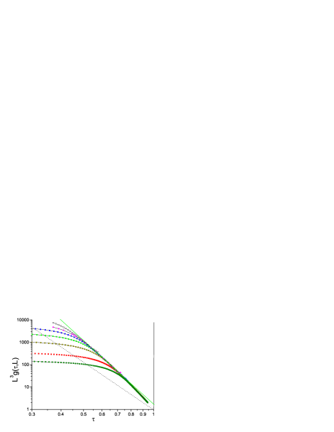
Figure 18: (Color on line) Dimension 3 Gaussian interaction ISG normalized Binder cumulant against $\tau$ for $L=32$, $24$, $20$, $16$, $12$, $8$, $6$ (top to bottom). Dashed line : slope $7.15=3\nu$, full green line slope $9.5$.

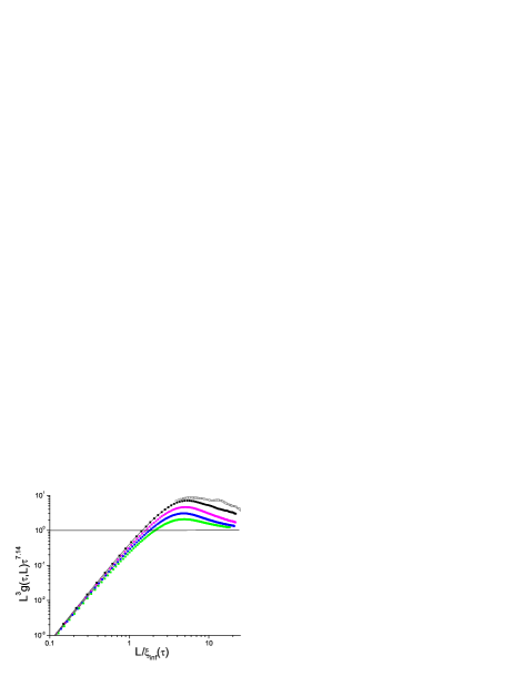
Figure 19: (Color on line) Dimension 3 Gaussian interaction ISG normalized Binder cumulant Privman-Fisher scaling assuming hyperscaling. Sizes shown are $L=32$, $20$, $10$, $6$, $4$ (top to bottom).

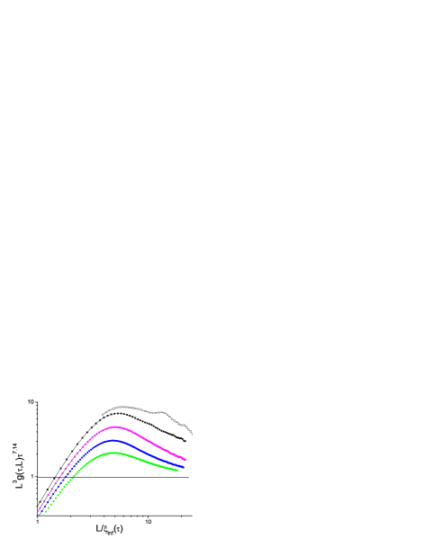
Figure 20: (Color on line) Dimension 3 Gaussian interaction ISG normalized Binder cumulant Privman-Fisher scaling assuming hyperscaling. Sizes shown are $L=32$, $20$, $10$, $6$, $4$ (top to bottom). Zoom of Fig. 19.

There is a possible empirical rationalization of the ISG Binder cumulant behavior. The data show that the ISG correlation length follows the ThL rule $\xi(\tau)=T\tau^{-2.4}$ (so $\nu(\tau)\sim 2.4$) to a good approximation over the entire paramagnetic range of temperatures. If we assume that the observed ThL behavior $L^{3}g(\tau)\sim\tau^{-10.5}$ extends to criticality also, it is equivalent to assuming that the strong disorder modifies the rule $L^{3}g(\tau)\sim\tau^{-\nu D}$ to $L^{3}g(\tau)\sim\tau^{-\nu D_{\mathrm{eff}}}$ with $D_{\mathrm{eff}}\sim 4.5$. By analogy with the Ising dimension 5 formalism we can write $D_{\mathrm{eff}}=3/\hbox{\coppa}$ with $\hbox{\coppa}\sim 0.7$ for both bimodal and Gaussian ISGs, and the modified Privman-Fisher scalings of the normalized Binder cumulants (see Fig. 10 for 5D Ising) should then take the form $L^{3}g(\tau,L)/(\tau^{-3\nu/\hbox{\coppa}})$ against $L^{\hbox{\coppa}}/(T\tau^{-\nu})$. These plots are shown in Figs. 21 and 22 for the 3D bimodal and Gaussian ISGs respectively.

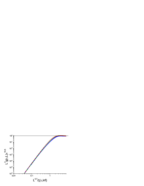
Figure 21: (Color on line) Dimension 3 bimodal ISG model. Normalized Binder cumulant $L^{3}g\tau^{10.5}$ against $L^{0.7}/\xi(\tau)$ for $L=24$ (cyan left triangle), $L=16$ (red inverted triangle), $L=12$ (green square), $L=8$ (pink triangle), $L=6$ (blue circle).

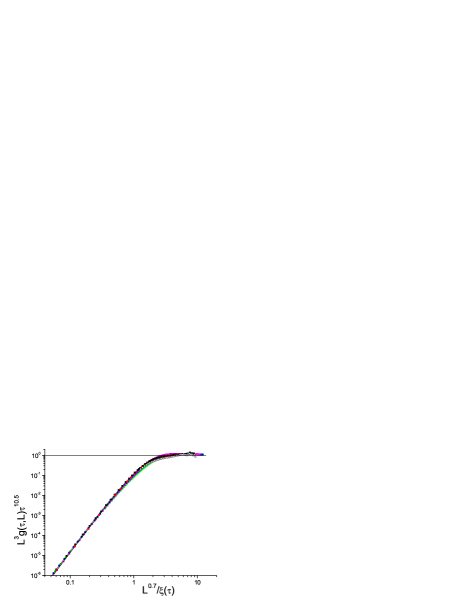
Figure 22: (Color on line) Dimension 3 Gaussian ISG model. Normalized Binder cumulant $L^{3}g\tau^{10.5}$ against $L^{0.7}/\xi(\tau)$ for $L=32$ (open circle), $L=24$ (cyan left triangle), $L=16$ (red inverted triangle), $L=10$ (pink triangle), $L=6$ (blue circle), $L=4$ (green square).

VIII Conclusion

The scaling of the susceptibility, the normalized correlation length, and the normalized Binder parameter are discussed for Ising models in dimensions 3 and 5, and for ISG models in dimension 3, using a rational normalization and scaling approach which covers the entire paramagnetic temperature region and not just the finite-size scaling regime.

For the canonical dimension 3 Ising model, the observed scaling of the normalized Binder cumulant $L^{D}g(\tau,L)$ is fully consistent with hyperscaling over the entire temperature range as to be expected. For the dimension 5 Ising model, above the upper critical dimension, the susceptibility, normalized correlation length, and normalized Binder cumulant scaling, are consistent with mean field exponents and so with the known breakdown of hyperscaling, over the entire temperature range including both the thermodynamic limit and the finite-size scaling regimes. The breakdowns of the two hyperscaling rules in dimension 5 conspire to ensure the size independence of the dimensionless Binder cumulant $g(\tau,L)$ at criticality.

In Ising spin glasses in dimension 3 the normalized Binder cumulant scaling shows a clear breakdown of the standard scaling rule in all the thermodynamic limit regime attainable with the available computational facilities; there is a return to behavior compatible with hyperscaling in the finite-size scaling regime at the approach to criticality. As no such breakdown is observed for the other observables, $\chi(\tau,L)$ and $\xi(\tau,L)T$, where hyperscaling is not involved, we propose that this behavior is the consequence of a Schwartz hyperscaling breakdown. Fuller characterization would require measurements to significantly higher sizes.

In the dimension 3 ISGs the ThL regime scaling is of the form $L^{D}g(\tau,L)\sim\tau^{q}$ with an effective exponent $q$ which is significantly higher than the hyperscaling value $q=D$. This scaling rule, with hyperscaling breakdown for the Binder cumulant only, implies $g(\tau_{c},L)\sim L^{D-q}$ at criticality and so is incompatible with the $g(\tau_{c},L)$ independent of $L$ observed in ISGs. We can postulate that in ISGs the fundamental physical rule concerning the size independence at criticality of dimensionless observables such as the Binder cumulant overrides the thermodynamic limit scaling rule at and close to criticality.

- (1) K. Binder, Z. Physik B 43, 119 (1981); Phys. Rev. Lett. 47, 693 (1981).
- (2) F. J. Wegner, Phys. Rev. B 5, 4529 (1972).
- (3) V. Privman, P. C. Hohenberg and A. Aharony, ”Universal Critical-Point Amplitude Relations”, in ”Phase Transitions and Critical Phenomena” (Academic, NY, 1991), eds. C. Domb and J. L. Lebowitz, 14, 1.
- (4) I. A. Campbell, K. Hukushima, and H. Takayama, Phys. Rev. Lett. 97, 117202 (2006).
- (5) M. Hasenbusch, A. Pelissetto and E. Vicari, Phys. Rev. B 78, 214205 (2008).
- (6) R. R. P. Singh and S. Chakravarty, Phys. Rev. Lett. 57, 245 (1986).
- (7) L. Klein, J. Adler, A. Aharony, A. B. Harris and Y. Meir, Phys. Rev. B 43, 11249 (1991).
- (8) D. Daboul, I. Chang, and A. Aharony, Eur. Phys. J. B 41, 231 (2004).
- (9) P. H. Lundow and I. A. Campbell, Phys. Rev.E 91, 042121 (2015).
- (10) P. Butera and M. Comi, Phys. Rev. B 65, 144431 (2002).
- (11) B. D. Josephson, Phys. Lett. 21, 608 (1966).
- (12) B. Widom, J. Chem. Phys. 43, 3892 (1965).
- (13) , L. P. Kadanoff, Physics (Long Island City) 2 263 (1966).
- (14) B. Simons, Phase Transitions and Collective Phenomena, Cambridge University Press (1997).
- (15) M. Schwartz, Europhys.Lett. 15, 777 (1991).
- (16) M. Gofman, J. Adler, A. Aharony, A. B. Harris, and M. Schwartz, Phys. Rev. Lett. 71, 1569 (1993).
- (17) R. L. C. Vink, T. Fischer, and K. Binder, Phys. Rev. E 82, 051134 (2010).
- (18) N. G. Fytas and V. Martin-Mayor, Phys. Rev. Lett. 110, 227201 (2013).
- (19) P. H. Lundow and I. A. Campbell, Physica A 434, 181 (2015).
- (20) D. Simmons-Duffin, JHEP 1506, 174 (2015).
- (21) R. Häggkvist, A. Rosengren, P. H. Lundow, K. Markström, D. Andrén, and P. Kundrotas, (2007), Adv. Phys. 56, 653 (2007).
- (22) I. A. Campbell and P. H. Lundow, Phys. Rev. B 83, 014411 (2011).
- (23) E. Luijten, H. W. J. Blöte, and K. Binder, Phys. Rev. Lett. 79, 561 (1997).
- (24) P. H. Lundow and I. A. Campbell, Phys. Rev. B 83, 184408 (2011).
- (25) P. Butera and M. Comi, J. Stat. Phys. 109, 311 (2002).
- (26) P. H. Lundow and I. A. Campbell, unpublished
- (27) T. Jörg, Phys. Rev. B 73, 224431 (2006).
- (28) B. Berche, R. Kenna and J. -C. Walter, Nucl. Phys. B 865 115 (2012).
- (29) J. L. Jones and A. P. Young, Phys. Rev. B 83, 014411 (2011).
- (30) P. Butera and M. Pernici, Phys. Rev. E 85 01105 (2012).
- (31) P. Butera and M. Pernici, Phys. Rev. E 86, 011139 (2012).
- (32) B. Berche, C. Chatelain, C. Dhall, R. Kenna, R. Low and J. C. Walter, J. Stat. Mech. (2008) P11010.
- (33) I. A. Campbell and P. Butera, Phys. Rev. B 78, 024435 (2008).
- (34) H. G. Katzgraber, M. Körner, and A. P. Young, Phys. Rev. B 73, 224432 (2006).
- (35) M. Baity-Jesi et al., Phys. Rev. B 88, 224416 (2013).
- (36) A. Pelissetto and E. Vicari, Phys. Rept. 368, 549 (2002).