Reinforcement Learning under Model Mismatch

Abstract

We study reinforcement learning under model misspecification, where we do not have access to the true environment but only to a reasonably close approximation to it. We address this problem by extending the framework of robust MDPs of [2, 17, 13] to the model-free Reinforcement Learning setting, where we do not have access to the model parameters, but can only sample states from it. We define robust versions of $\operatorname{Q}$-learning, $\operatorname{SARSA}$, and $\operatorname{TD}$-learning and prove convergence to an approximately optimal robust policy and approximate value function respectively. We scale up the robust algorithms to large MDPs via function approximation and prove convergence under two different settings. We prove convergence of robust approximate policy iteration and robust approximate value iteration for linear architectures (under mild assumptions). We also define a robust loss function, the mean squared robust projected Bellman error and give stochastic gradient descent algorithms that are guaranteed to converge to a local minimum.

1 Introduction

Reinforcement learning is concerned with learning a good policy for sequential decision making problems modeled as a Markov Decision Process (MDP), via interacting with the environment [22, 20]. In this work we address the problem of reinforcement learning from a misspecified model. As a motivating example, consider the scenario where the problem of interest is not directly accessible, but instead the agent can interact with a simulator whose dynamics is reasonably close to the true problem. Another plausible application is when the parameters of the model may evolve over time but can still be reasonably approximated by an MDP.

To address this problem we use the framework of robust MDPs which was proposed by [2, 17, 13] to solve the planning problem under model misspecification. The robust MDP framework considers a class of models and finds the robust optimal policy which is a policy that performs best under the worst model. It was shown by [2, 17, 13] that the robust optimal policy satisfies the robust Bellman equation which naturally leads to exact dynamic programming algorithms to find an optimal policy. However, this approach is model dependent and does not immediately generalize to the model-free case where the parameters of the model are unknown.

Essentially, reinforcement learning is a model-free framework to solve the Bellman equation using samples. Therefore, to learn policies from misspecified models, we develop sample based methods to solve the robust Bellman equation. In particular, we develop robust versions of classical reinforcement learning algorithms such as $\operatorname{Q}$-learning, $\operatorname{SARSA}$, and $\operatorname{TD}$-learning and prove convergence to an approximately optimal policy under mild assumptions on the discount factor. We also show that the nominal versions of these iterative algorithms converge to policies that may be arbitrarily worse compared to the optimal policy.

We also scale up these robust algorithms to large scale MDPs via function approximation, where we prove convergence under two different settings. Under a technical assumption similar to [6, 26] we show convergence of robust approximate policy iteration and value iteration algorithms for linear architectures. We also study function approximation with nonlinear architectures, by defining an appropriate mean squared robust projected Bellman error (MSRPBE) loss function, which is a generalization of the mean squared projected Bellman error (MSPBE) loss function of [23, 24, 7]. We propose robust versions of stochastic gradient descent algorithms as in [23, 24, 7] and prove convergence to a local minimum under some assumptions for function approximation with arbitrary smooth functions.

Contribution.

In summary we have the following contributions:

1. We extend the robust MDP framework of [2, 17, 13] to the model-free reinforcement learning setting. We then define robust versions of $\operatorname{Q}$-learning, $\operatorname{SARSA}$, and $\operatorname{TD}$-learning and prove convergence to an approximately optimal robust policy.

2. We also provide robust reinforcement learning algorithms for the function approximation case and prove convergence of robust approximate policy iteration and value iteration algorithms for linear architectures. We also define the MSRPBE loss function which contains the robust optimal policy as a local minimum and we derive stochastic gradient descent algorithms to minimize this loss function as well as establish convergence to a local minimum in the case of function approximation by arbitrary smooth functions.

3. Finally, we demonstrate empirically the improvement in performance for the robust algorithms compared to their nominal counterparts. For this we used various Reinforcement Learning test environments from OpenAI [10] as benchmark to assess the improvement in performance as well as to ensure reproducibility and consistency of our results.

Related Work.

Recently, several approaches have been proposed to address model performance due to parameter uncertainty for Markov Decision Processes (MDPs). A Bayesian approach was proposed by [21] which requires perfect knowledge of the prior distribution on transition matrices. Other probabilistic and risk based settings were studied by [11, 28, 25] which propose various mechanisms to incorporate percentile risk into the model. A framework for robust MDPs was first proposed by [2, 17, 13] who consider the transition matrices to lie in some uncertainty set and proposed a dynamic programming algorithm to solve the robust MDP. Recent work by [26] extended the robust MDP framework to the function approximation setting where under a technical assumption the authors prove convergence to an optimal policy for linear architectures. Note that these algorithms for robust MDPs do not readily generalize to the model-free reinforcement learning setting where the parameters of the environment are not explicitly known.

For reinforcement learning in the non-robust model-free setting, several iterative algorithms such as $\operatorname{Q}$-learning, $\operatorname{TD}$-learning, and $\operatorname{SARSA}$ are known to converge to an optimal policy under mild assumptions, see [5] for a survey. Robustness in reinforcement learning for MDPs was studied by [15] who introduced a robust learning framework for learning with disturbances. Similarly, [18] also studied learning in the presence of an adversary who might apply disturbances to the system. However, for the algorithms proposed in [15, 18] no theoretical guarantees are known and there is only limited empirical evidence. Another recent work on robust reinforcement learning is [14], where the authors propose an online algorithm with certain transitions being stochastic and the others being adversarial and the devised algorithm ensures low regret.

For the case of reinforcement learning with large MDPs using function approximations, theoretical guarantees for most $\operatorname{TD}$-learning based algorithms are only known for linear architectures [3]. Recent work by [7] extended the results of [23, 24] and proved that a stochastic gradient descent algorithm minimizing the mean squared projected Bellman equation (MSPBE) loss function converges to a local minimum, even for nonlinear architectures. However, these algorithms do not apply to robust MDPs; in this work we extend these algorithms to the robust setting.

2 Preliminaries

We consider an infinite horizon Markov Decision Process (MDP) [20] with finite state space $\mathcal{X}$ of size $n$ and finite action space $\mathcal{A}$ of size $m$. At every time step $t$ the agent is in a state $i\in\mathcal{X}$ and can choose an action $a\in\mathcal{A}$ incurring a cost $c_{t}(i,a)$. We will make the standard assumption that future cost is discounted, see e.g., [22], with a discount factor $\vartheta<1$ applied to future costs, i.e., $c_{t}(i,a)\coloneqq\vartheta^{t}c(i,a),$ where $c(i,a)$ is a fixed constant independent of the time step $t$ for $i\in\mathcal{X}$ and $a\in\mathcal{A}$. The states transition according to probability transition matrices $\tau\coloneqq\left\{P^{a}\right\}_{a\in\mathcal{A}}$ which depends only on their last taken action $a$. A policy of the agent is a sequence $\pi=\left(\mathbf{a_{0}},\mathbf{a_{1}},\dots\right)$, where every $\mathbf{a_{t}}(i)$ corresponds to an action in $\mathcal{A}$ if the system is in state $i$ at time $t$. For every policy $\pi$, we have a corresponding value function $v_{\pi}\in\mathbb{R}^{n}$, where $v_{\pi}(i)$ for a state $i\in\mathcal{X}$ measures the expected cost of that state if the agent were to follow policy $\pi$. This can be expressed by the following recurrence relation

$$v_{\pi}(i)\coloneqq c(i,\mathbf{a}_{0}(i))+\vartheta\mathbb{E}_{j\sim\mathcal{X}}\left[v_{\pi}(j)\right].$$ (1)

The goal is to devise algorithms to learn an optimal policy $\pi^{*}$ that minimizes the expected total cost:

Definition 2.1 (Optimal policy).

Given an MDP with state space $\mathcal{X}$, action space $\mathcal{A}$ and transition matrices $P^{a}$, let $\Pi$ be the strategy space of all possibile policies. Then an optimal policy $\pi^{*}$ is one that minimizes the expected total cost, i.e., $\pi^{*}\coloneqq\arg\min_{\pi\in\Pi}\mathbb{E}\left[\sum_{t=0}^{\infty}\vartheta^{t}c(i_{t},\mathbf{a_{t}}(i_{t}))\right].$

In the robust case we will assume as in [17, 13] that the transition matrices $P^{a}$ are not fixed and may come from some uncertainty region $\mathcal{P}^{a}$ and may be chosen adversarially by nature in future runs of the model. In this setting, [17, 13] prove the following robust analogue of the Bellman recursion. A policy of nature is a sequence $\tau\coloneqq\left(\mathbf{P_{0}},\mathbf{P_{1}},\dots\right)$ where every $P_{t}(a)\in\mathcal{P}^{a}$ corresponds to a transition probability matrix chosen from $\mathcal{P}^{a}$. Let $\mathcal{T}$ denote the set of all such policies of nature. In other words, a policy $\tau\in\mathcal{T}$ of nature is a sequence of transition matrices that may be played by it in response to the actions of the agent. For any set $P\subseteq\mathbb{R}^{n}$ and vector $v\in\mathbb{R}^{n}$, let $\sigma_{P}(v)\coloneqq\sup\left\{p^{\top}v\mid p\in P\right\}$ be the support function of the set $P$. For a state $i\in\mathcal{X}$, let $\mathcal{P}^{a}_{i}$ be the projection onto the $i^{th}$ row of $\mathcal{P}^{a}$.

Theorem 2.2.

[17] We have the following perfect duality relation

$$\min_{\pi\in\Pi}\max_{\tau\in\mathcal{T}}\mathbb{E}_{\tau}\left[\sum_{t=0}^{\infty}\vartheta^{t}c\left(i_{t},\mathbf{a_{t}}(i_{t})\right)\right]=\max_{\tau\in\mathcal{T}}\min_{\pi\in\Pi}\mathbb{E}_{\tau}\left[\sum_{t=0}^{\infty}\vartheta^{t}c\left(i_{t},\mathbf{a_{t}}(i_{t})\right)\right].$$ (2)

The optimal value function $v_{\pi^{*}}$ corresponding to the optimal policy $\pi^{*}$ satisfies

$$v_{\pi^{*}}(i)=\min_{a\in\mathcal{A}}\left(c(i,a)+\vartheta\sigma_{\mathcal{P}^{a}_{i}}(v_{\pi^{*}})\right),$$ (3)

and $\pi^{*}$ can then be obtained in a greedy fashion, i.e., $\mathbf{a}^{*}(i)\in\arg\min_{a\in\mathcal{A}}\left\{c(i,a)+\vartheta\sigma_{\mathcal{P}^{a}_{i}}(v)\right\}.$

The main shortcoming of this approach is that it does not generalize to the model free case where the transition probabilities are not explicitly known but rather the agent can only sample states according to these probabilities. In the absence of this knowledge, we cannot compute the support functions of the uncertainty sets $\mathcal{P}^{a}_{i}$. On the other hand it is often easy to have a confidence region $U^{a}_{i}$, e.g., a ball or an ellipsoid, corresponding to every state-action pair $i\in\mathcal{X},a\in\mathcal{A}$ that quantifies our uncertainty in the simulation, with the uncertainty set $\mathcal{P}^{a}_{i}$ being the confidence region $U^{a}_{i}$ centered around the unknown simulator probabilities. Formally, we define the uncertainty sets corresponding to every state action pair in the following fashion.

Definition 2.3 (Uncertainty sets).

Corresponding to every state-action pair $(i,a)$ we have a confidence region $U^{a}_{i}$ so that the uncertainty region $\mathcal{P}^{a}_{i}$ of the probability transition matrix corresponding to $(i,a)$ is defined as

$$\mathcal{P}^{a}_{i}\coloneqq\left\{x+p^{a}_{i}\mid x\in U^{a}_{i}\right\},$$ (4)

where $p^{a}_{i}$ is the unknown state transition probability vector from the state $i\in\mathcal{X}$ to every other state in $\mathcal{X}$ given action $a$ during the simulation.

As a simple example, we have the ellipsoid $U^{a}_{i}\coloneqq\left\{x\mid x^{\top}A^{a}_{i}x\leq 1,\sum_{i\in\mathcal{X}}x_{i}=0\right\}$ for some $n\times n$ psd matrix $A^{a}_{i}$ with the uncertainty set $\mathcal{P}^{a}_{i}$ being $\mathcal{P}^{a}_{i}\coloneqq\left\{x+p^{a}_{i}\mid x\in U^{a}_{i}\right\},$ where $p^{a}_{i}$ is the unknown simulator state transition probability vector with which the agent transitioned to a new state during training. Note that while it may easy to come up with good descriptions of the confidence region $U^{a}_{i}$, the approach of [17, 13] breaks down since we have no knowledge of $p^{a}_{i}$ and merely observe the new state $j$ sampled from this distribution. See Figure 1 for an illustration with the confidence regions being an $\ell_{2}$ ball of fixed radius $r$.

In the following sections we develop robust versions of $\operatorname{Q}$-learning, $\operatorname{SARSA}$, and $\operatorname{TD}$-learning which are guaranteed to converge to an approximately optimal policy that is robust with respect to this confidence region. The robust versions of these iterative algorithms involve an additional linear optimization step over the set $U^{a}_{i}$, which in the case of $U^{a}_{i}=\left\{\left\|x\right\|_{2}\leq r\right\}$ simply corresponds to adding fixed noise during every update. In later sections we will extend it to the function approximation case where we study linear architectures as well as nonlinear architectures; in the latter case we derive new stochastic gradient descent algorithms for computing approximately robust policies.

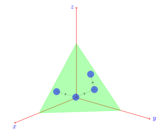
Figure 1: Example transition matrices shown within the probability simplex $\Delta_{n}$ with uncertainty sets being $\ell_{2}$ balls of fixed radius.

3 Robust exact dynamic programming algorithms

In this section we develop robust versions of exact dynamic programming algorithms such as $\operatorname{Q}$-learning, $\operatorname{SARSA}$, and $\operatorname{TD}$-learning. These methods are suitable for small MDPs where the size $n$ of the state space is not too large. Note that confidence region $U^{a}_{i}$ must also be constrained to lie within the probability simplex $\Delta_{n}$, see Figure 1. However since we do not have knowledge of the simulator probabilities $p^{a}_{i}$, we do not know how far away $p^{a}_{i}$ is from the boundary of $\Delta_{n}$ and so the algorithms will make use of a proxy confidence region $\widehat{U^{a}_{i}}$ where we drop the requirement of $\widehat{U^{a}_{i}}\subseteq\Delta_{n}$, to compute the robust optimal policies. With a suitable choice of step lengths and discount factors we can prove convergence to an approximately optimal $U^{a}_{i}$-robust policy where the approximation depends on the difference between the unconstrained proxy region $\widehat{U^{a}_{i}}$ and the true confidence region $U^{a}_{i}$. Below we give specific examples of possible choices for simple confidence regions.

1. Ellipsoid: Let $\{A^{a}_{i}\}_{i,a}$ be a sequence of $n\times n$ psd matrices. Then we can define the confidence region as

   $$U^{a}_{i}\coloneqq\left\{x\middle|x^{\top}A^{a}_{i}x\leq 1,\sum_{i\in\mathcal{X}}x_{i}=0,-p^{a}_{ij}\leq x_{j}\leq 1-p^{a}_{ij},\forall j\in\mathcal{X}\right\}.$$ (5)

   Note that $U^{a}_{i}$ has some additional linear constraints so that the uncertainty set $\mathcal{P}^{a}_{i}\coloneqq\left\{p^{a}_{i}+x\mid x\in U^{a}_{i}\right\}$ lies inside $\Delta_{n}$. Since we do not know $p^{a}_{i}$, we will make use of the proxy confidence region $\widehat{U^{a}_{i}}\coloneqq\{x\mid x^{\top}A^{a}_{i}x\leq 1,\sum_{i\in\mathcal{X}}x_{i}=0\}$. In particular when $A^{a}_{i}=r^{-1}I_{n}$ for every $i\in\mathcal{X},a\in\mathcal{A}$ then this corresponds to a spherical confidence interval of $[-r,r]$ in every direction. In other words, each uncertainty set $\mathcal{P}^{a}_{i}$ is an $\ell_{2}$ ball of radius $r$.

2. Parallelepiped: Let $\{B^{a}_{i}\}_{i,a}$ be a sequence of $n\times n$ invertible matrices. Then we can define the confidence region as

   $$U^{a}_{i}\coloneqq\left\{x\middle|\left\|B^{a}_{i}x\right\|_{1}\leq 1,\sum_{i\in\mathcal{X}}x_{i}=0,-p^{a}_{ij}\leq x_{j}\leq 1-p^{a}_{ij},\forall j\in\mathcal{X}\right\}.$$ (6)

   As before, we will use the unconstrained parallelepiped $\widehat{U^{a}_{i}}$ without the $-p^{a}_{ij}\leq x_{j}\leq 1-p^{a}_{ij}$ constraints, as a proxy for $U^{a}_{i}$ since we do not have knowledge $p^{a}_{i}$. In particular if $B^{a}_{i}=D$ for a diagonal matrix $D$, then the proxy confidence region $\widehat{U^{a}_{i}}$ corresponds to a rectangle. In particular if every diagonal entry is $r$, then every uncertainty set $\mathcal{P}^{a}_{i}$ is an $\ell_{1}$ ball of radius $r$.

3.1 Robust $\operatorname{Q}$-learning

Let us recall the notion of a $\operatorname{Q}$-factor of a state-action pair $(i,a)$ and a policy $\pi$ which in the non-robust setting is defined as

$$\operatorname{Q}(i,a)\coloneqq c(i,a)+\mathbb{E}_{j\sim\mathcal{X}}\left[v(j)\right],$$ (7)

where $v$ is the value function of the policy $\pi$. In other words, the $\operatorname{Q}$-factor represents the expected cost if we start at state $i$, use the action $a$ and follow the policy $\pi$ subsequently. One may similarly define the robust $\operatorname{Q}$-factors using a similar interpretation and the minimax characterization of Theorem 2.2. Let $\operatorname{Q}^{*}$ denote the $\operatorname{Q}$-factors of the optimal robust policy and let $v^{*}\in\mathbb{R}^{n}$ be its value function. Note that we may write the value function in terms of the $\operatorname{Q}$-factors as $v^{*}=\min_{a\in\mathcal{A}}\operatorname{Q}^{*}(i,a)$. From Theorem 2.2 we have the following expression for $\operatorname{Q}^{*}$:

$$\operatorname{Q}^{*}(i,a) =c(i,a)+\vartheta\sigma_{\mathcal{P}^{a}_{i}}(v^{*})$$ (8)

$$=c(i,a)+\vartheta\sigma_{U^{a}_{i}}(v^{*})+\vartheta\sum_{j\in\mathcal{X}}p^{a}_{ij}\min_{a^{\prime}\in\mathcal{A}}\operatorname{Q}^{*}(j,a^{\prime}),$$ (9)

where equation (9) follows from Definition 2.3. For an estimate $\operatorname{Q}_{t}$ of $\operatorname{Q}^{*}$, let $v_{t}\in\mathbb{R}^{n}$ be its value vector, i.e., $v_{t}(i)\coloneqq\min_{a\in\mathcal{A}}\operatorname{Q}_{t}(i,a)$. The robust $\operatorname{Q}$-iteration is defined as:

$$\operatorname{Q}_{t}(i,a)\coloneqq(1-\gamma_{t})\operatorname{Q}_{t-1}(i,a)+\gamma_{t}\left(c(i,a)+\vartheta\sigma_{\widehat{U^{a}_{i}}}\left(v_{t-1}\right)+\vartheta\min_{a^{\prime}\in\mathcal{A}}\operatorname{Q}_{t-1}(j,a^{\prime})\right),$$ (10)

where a state $j\in\mathcal{X}$ is sampled with the unknown transition probability $p^{a}_{ij}$ using the simulator. Note that the robust $\operatorname{Q}$-iteration of equation (10) involves an additional linear optimization step to compute the support function $\sigma_{\widehat{U^{a}_{i}}}(v_{t})$ of $v_{t}$ over the proxy confidence region $\widehat{U^{a}_{i}}$. We will prove that iterating equation (10) converges to an approximately optimal policy. The following definition introduces the notion of an $\varepsilon$-optimal policy, see e.g., [5]. The error factor $\varepsilon$ is also referred to as the amplification factor. We will treat the $\operatorname{Q}$-factors as a $\left|\mathcal{X}\right|\times\left|\mathcal{A}\right|$ matrix in the definition so that its $\ell_{\infty}$ norm is defined as usual.

Definition 3.1 ($\varepsilon$-optimal policy).

A policy $\pi$ with $\operatorname{Q}$-factors $\operatorname{Q}^{\prime}$ is $\varepsilon$-optimal with respect to the optimal policy $\pi^{*}$ with corresponding $\operatorname{Q}$-factors $\operatorname{Q}^{*}$ if

$$\left\|\operatorname{Q}^{\prime}-\operatorname{Q}^{*}\right\|_{\infty}\leq\varepsilon\left\|\operatorname{Q}^{*}\right\|_{\infty}.$$ (11)

The following simple lemma allows us to decompose the optimization of a linear function over the proxy uncertainty set $\widehat{\mathcal{P}^{a}_{i}}$ in terms of linear optimization over $\mathcal{P}^{a}_{i},U^{a}_{i}$, and $\widehat{U^{a}_{i}}$.

Lemma 3.2.

Let $v\in\mathbb{R}^{n}$ be any vector and let $\beta^{a}_{i}\coloneqq\max_{y\in\widehat{U^{a}_{i}}}\min_{x\in U^{a}_{i}}\left\|y-x\right\|_{1}$. Then we have $\sigma_{\widehat{\mathcal{P}^{a}_{i}}}(v)\leq\sigma_{\mathcal{P}^{a}_{i}}(v)+\beta^{a}_{i}\left\|v\right\|_{\infty}.$

Proof.

Note that every point $p$ in $\mathcal{P}^{a}_{i}$ is of the form $p^{a}_{i}+x$ for some $x\in U^{a}_{i}$ and every point $q\in\widehat{\mathcal{P}^{a}_{i}}$ is of the form $p^{a}_{i}+y$ for some $y\in\widehat{U^{a}_{i}}$, and this correspondence is one to one by definition. For any vector $v\in\mathbb{R}^{n}$ and pairs of points $p\in\mathcal{P}^{a}_{i}$ and $q\in\widehat{\mathcal{P}^{a}_{i}}$ we have

$$q^{\top}v =p^{\top}v+(q-p)^{\top}v$$ (12)

$$\leq\sup_{p^{\prime}\in\mathcal{P}^{a}_{i}}(p^{\prime})^{\top}v+\left(p^{a}_{i}+y-p^{a}_{i}-x\right)^{\top}v$$ (13)

$$=\sigma_{\mathcal{P}^{a}_{i}}(v)+(y-x)^{\top}v.$$ (14)

$$\leq\sigma_{\mathcal{P}^{a}_{i}}(v)+(y-x)^{\top}v$$ (15)

$$\leq\sigma_{\mathcal{P}^{a}_{i}}(v)+\left(y^{\top}v-\min_{x\in U^{a}_{i}}x^{\top}v\right)$$ (16)

$$\leq\sigma_{\mathcal{P}^{a}_{i}}(v)+\max_{y\in\widehat{U^{a}_{i}}}\min_{x\in U^{a}_{i}}(y-x)^{\top}v$$ (17)

$$\leq\sigma_{\mathcal{P}^{a}_{i}}(v)+\max_{y\in\widehat{U^{a}_{i}}}\min_{x\in U^{a}_{i}}\left\|y-x\right\|_{1}\left\|v\right\|_{\infty}$$ (18)

$$\leq\sigma_{\mathcal{P}^{a}_{i}}(v)+\beta^{a}_{i}\left\|v\right\|_{\infty}.$$ (19)

Since equation (19) holds for every $q\in\widehat{\mathcal{P}^{a}_{i}}$, it follows that it also holds for $\arg\max\sigma_{\widehat{\mathcal{P}^{a}_{i}}}(v)$ so that

$$\sigma_{\widehat{\mathcal{P}^{a}_{i}}}(v)\leq\sigma_{\mathcal{P}^{a}_{i}}(v)+\beta^{a}_{i}\left\|v\right\|_{\infty}.$$ (20)

∎

The following theorem proves that under a suitable choice of step lengths $\gamma_{t}$ and discount factor $\vartheta$, the iteration of equation (10) converges to an $\varepsilon$-approximately optimal policy with respect to the confidence regions $U^{a}_{i}$.

Theorem 3.3.

Let the step lengths $\gamma_{t}$ of the $\operatorname{Q}$-iteration algorithm be chosen such that $\sum_{t=0}^{\infty}\gamma_{t}=\infty$ and $\sum_{t=0}^{\infty}\gamma_{t}^{2}<\infty$ and let the discount factor $\vartheta<1$. Let $\beta^{a}_{i}$ be as in Lemma 3.2 and let $\beta\coloneqq\max_{i\in\mathcal{X},a\in\mathcal{A}}\beta^{a}_{i}$. If $\vartheta(1+\beta)<1$ then with probability $1$ the iteration of equation (10) converges to an $\varepsilon$-optimal policy where $\varepsilon\coloneqq\frac{\vartheta\beta}{1-\vartheta\left(1+\beta\right)}.$

Proof.

Let $\widehat{\mathcal{P}^{a}_{i}}$ be the proxy uncertainty set for state $i\in\mathcal{X}$ and $a\in\mathcal{A}$, i.e., $\widehat{\mathcal{P}^{a}_{i}}\coloneqq\left\{x+p^{a}_{i}\mid x\in\widehat{U^{a}_{i}}\right\}$. We denote the value function of $\operatorname{Q}$ by $v$. Let us define the following operator $H$ mapping $\operatorname{Q}$-factors to $\operatorname{Q}$-factors as follows:

$$(H\operatorname{Q})(i,a) \coloneqq c(i,a)+\vartheta\sigma_{\widehat{\mathcal{P}^{a}_{i}}}(v).$$ (21)

We will first show that a solution $\operatorname{Q}^{\prime}$ to the equation $H\operatorname{Q}=\operatorname{Q}$ is an $\varepsilon$-optimal policy as in Definition 3.1, i.e., $\left\|Q^{\prime}-Q^{*}\right\|_{\infty}\leq\varepsilon\left\|Q^{*}\right\|_{\infty}$.

$$|\operatorname{Q}^{\prime}(i,a)-\operatorname{Q}^{*}(i,a)| =\left|(H\operatorname{Q}^{\prime})(i,a)-c(i,a)-\vartheta\sigma_{\mathcal{P}^{a}_{i}}(v^{*})\right|$$ (22)

$$=\vartheta\left|\sigma_{\widehat{\mathcal{P}^{a}_{i}}}(v^{\prime})-\sigma_{\mathcal{P}^{a}_{i}}(v^{*})\right|$$ (23)

$$\leq\vartheta\left|\max_{y\in\widehat{U^{a}_{i}},x\in U^{a}_{i}}\left\|y-x\right\|_{1}\left\|\operatorname{Q}^{\prime}\right\|_{\infty}+\sigma_{\mathcal{P}^{a}_{i}}(v^{\prime})-\sigma_{\mathcal{P}^{a}_{i}}(v^{*})\right|$$ (24)

$$\leq\vartheta\beta^{a}_{i}\left\|\operatorname{Q}^{\prime}\right\|_{\infty}+\left|\sigma_{\mathcal{P}^{a}_{i}}(v^{\prime})-\sigma_{\mathcal{P}^{a}_{i}}(v^{*})\right|$$ (25)

$$\leq\vartheta\beta\left\|\operatorname{Q}^{\prime}\right\|_{\infty}+\vartheta\left|\max_{q^{\prime}\in\mathcal{P}^{a}_{i}}\sum_{j\in\mathcal{X}}q^{\prime}_{j}\min_{a^{\prime\prime}\in\mathcal{A}}\operatorname{Q}^{\prime}(j,a^{\prime\prime})-\max_{q\in\mathcal{P}^{a}_{i}}\sum_{j\in\mathcal{X}}q_{j}\min_{a^{\prime}\in\mathcal{A}}\operatorname{Q}^{*}(j,a^{\prime})\right|$$ (26)

$$\leq\vartheta\beta\left\|\operatorname{Q}^{\prime}\right\|_{\infty}+\vartheta\left|\max_{q\in\mathcal{P}^{a}_{i}}\sum_{j\in\mathcal{X}}q_{j}\left(\min_{a^{\prime\prime}\in\mathcal{A}}\operatorname{Q}^{\prime}(j,a^{\prime\prime})-\min_{a^{\prime}\in\mathcal{A}}\operatorname{Q}^{*}(j,a^{\prime})\right)\right|$$ (27)

$$\leq\vartheta\beta\left\|\operatorname{Q}^{\prime}\right\|_{\infty}+\vartheta\left|\max_{q\in\mathcal{P}^{a}_{i}}\sum_{j\in\mathcal{X}}q_{j}\left(\max_{a^{\prime}\in\mathcal{A}}|\operatorname{Q}^{\prime}(j,a^{\prime})-\operatorname{Q}^{*}(j,a^{\prime})|\right)\right|$$ (28)

$$\leq\vartheta\beta\left\|\operatorname{Q}^{\prime}\right\|_{\infty}+\vartheta\left|\max_{q\in\mathcal{P}^{a}_{i}}\sum_{j\in\mathcal{X}}q_{j}\left\|\operatorname{Q}^{\prime}-\operatorname{Q}^{*}\right\|_{\infty}\right|$$ (29)

$$\leq\vartheta\beta\left\|\operatorname{Q}^{\prime}\right\|_{\infty}+\vartheta\left\|\operatorname{Q}^{\prime}-\operatorname{Q}^{*}\right\|_{\infty},$$ (30)

where we used Lemma 3.2 to derive equation (24). Equation (30) implies that $\left\|\operatorname{Q}^{\prime}-\operatorname{Q}^{*}\right\|_{\infty}\leq\frac{\vartheta\beta}{1-\vartheta}\left\|\operatorname{Q}^{\prime}\right\|_{\infty}$. If $\left\|\operatorname{Q}^{\prime}\right\|_{\infty}\leq\left\|\operatorname{Q}^{*}\right\|_{\infty}$ then we are done since $\frac{\vartheta\beta}{1-\vartheta}\leq\frac{\vartheta\beta}{1-\vartheta(1+\beta)}$. Otherwise assume that $\left\|\operatorname{Q}^{\prime}\right\|_{\infty}>\left\|\operatorname{Q}^{*}\right\|_{\infty}$ and use the triangle inequality: $\left\|\operatorname{Q}^{\prime}\right\|_{\infty}-\left\|\operatorname{Q}^{*}\right\|_{\infty}=\left|\left\|\operatorname{Q}^{\prime}\right\|_{\infty}-\left\|\operatorname{Q}^{*}\right\|_{\infty}\right|\leq\left\|\operatorname{Q}^{\prime}-\operatorname{Q}^{*}\right\|_{\infty}$. This implies that

$$\frac{1-\vartheta}{\vartheta\beta}\left\|\operatorname{Q}^{\prime}-\operatorname{Q}^{*}\right\|_{\infty}-\left\|\operatorname{Q}^{*}\right\|_{\infty}\leq\left\|\operatorname{Q}^{\prime}-\operatorname{Q}^{*}\right\|_{\infty},$$ (31)

from which it follows that $\left\|\operatorname{Q}^{\prime}-\operatorname{Q}^{*}\right\|_{\infty}\leq\varepsilon\left\|\operatorname{Q}^{*}\right\|_{\infty}$ under the assumption that $\vartheta(1+\beta)<1$ as claimed. The $\operatorname{Q}$-iteration of equation (10) can then be reformulated in terms of the operator $H$ as

$$\operatorname{Q}_{t}(i,a)=(1-\gamma_{t})\operatorname{Q}_{t-1}(i,a)+\gamma_{t}\left(H\operatorname{Q}_{t}(i,a)+\eta_{t}(i,a)\right),$$ (32)

where $\eta_{t}(i,a)\coloneqq\min_{a^{\prime}\in\mathcal{A}}\operatorname{Q}_{t}(j,a^{\prime})-\mathbb{E}_{j\sim p^{a}_{i}}\left[\min_{a^{\prime}\in\mathcal{A}}\operatorname{Q}_{t}(j,a^{\prime})\right]$ where the expectation is over the states $j\in\mathcal{X}$ with the transition probability from state $i$ to state $j$ given by $p^{a}_{j}$. Note that this is an example of a stochastic approximation algorithm as in [5] with noise parameter $\eta_{t}$. Let $\mathcal{F}_{t}$ denote the history of the algorithm until time $t$. Note that $\mathbb{E}_{j\sim p^{a}_{i}}\left[\eta_{t}(i,a)\middle|\mathcal{F}_{t}\right]=0$ by definition and the variance is bounded by

$$\mathbb{E}_{j\sim p^{a}_{i}}\left[\eta_{t}(i,a)^{2}\middle|\mathcal{F}_{t}\right]\leq K\left(1+\max_{\begin{subarray}{c}j\in\mathcal{X}\\ a^{\prime}\in\mathcal{A}\end{subarray}}\operatorname{Q}_{t}^{2}(j,a^{\prime})\right).$$ (33)

Thus the noise term $\eta_{t}$ satisfies the zero conditional mean and bounded variance assumption (Assumption 4.3 in [5]). Therefore it remains to show that the operator $H$ is a contraction mapping to argue that iterating equation (10) converges to the optimal $\operatorname{Q}$-factor $\operatorname{Q}^{*}$. We will show that the operator $H$ is a contraction mapping with respect to the infinity norm $\left\|.\right\|_{\infty}$. Let $\operatorname{Q}$ and $\operatorname{Q}^{\prime}$ be two different $\operatorname{Q}$-vectors with value functions $v$ and $v^{\prime}$. If $U^{a}_{i}$ is not necessarily the same as the unconstrained proxy set $\widehat{U^{a}_{i}}$ for some $i\in\mathcal{X},a\in\mathcal{A}$, then we need the discount factor to satisfy $\vartheta(1+\beta)$ in order to ensure convergence. Intuitively, the discount factor should be small enough that the difference in the estimation due to the difference of the sets $U^{a}_{i}$ and $\widehat{U^{a}_{i}}$ converges to $0$ over time. In this case we show contraction for operator $H$ as follows

$$|(H\operatorname{Q})(i,a)-(H\operatorname{Q}^{\prime})(i,a)| \leq\vartheta\left|\max_{q\in\widehat{\mathcal{P}^{a}_{i}}}\sum_{j\in\mathcal{X}}q_{j}\left(\min_{a^{\prime}\in\mathcal{A}}\operatorname{Q}(j,a^{\prime})-\min_{a^{\prime\prime}\in\mathcal{A}}\operatorname{Q}^{\prime}(j,a^{\prime\prime})\right)\right|$$ (34)

$$\leq\vartheta\max_{q\in\widehat{\mathcal{P}^{a}_{i}}}\sum_{j\in\mathcal{X}}q_{j}\max_{a^{\prime}\in\mathcal{A}}\left|Q(j,a^{\prime})-\operatorname{Q}^{\prime}(j,a^{\prime})\right|$$ (35)

$$\leq\vartheta\max_{y\in\widehat{U},x\in U}\left\|y-x\right\|_{1}\left\|\operatorname{Q}-\operatorname{Q}^{\prime}\right\|_{\infty}+\vartheta\max_{q\in\mathcal{P}^{a}_{i}}\sum_{j\in\mathcal{X}}q_{j}\left\|\operatorname{Q}-\operatorname{Q}^{\prime}\right\|_{\infty}$$ (36)

$$\leq\vartheta\beta\left\|\operatorname{Q}-\operatorname{Q}^{\prime}\right\|_{\infty}+\vartheta\left\|\operatorname{Q}-\operatorname{Q}^{\prime}\right\|_{\infty}\max_{q\in\mathcal{P}^{a}_{i}}\sum_{j\in\mathcal{X}}q_{j}$$ (37)

$$\leq\vartheta(\beta+1)\left\|\operatorname{Q}-\operatorname{Q}^{\prime}\right\|_{\infty}$$ (38)

where we used Lemma 3.2 with vector $v(j)\coloneqq\max_{a\in\mathcal{A}}\left|Q(j,a)-Q^{\prime}(j,a)\right|$ to derive equation (36) and the fact that $\mathcal{P}^{a}_{i}\subseteq\Delta_{n}$ to conclude that $\max_{q\in\mathcal{P}^{a}_{i}}\sum_{j\in\mathcal{X}}q_{j}=1$. Therefore if $\vartheta(1+\beta)<1$, then it follows that the operator $H$ is a norm contraction and thus the robust $\operatorname{Q}$-iteration of equation (10) converges to a solution of $H\operatorname{Q}=\operatorname{Q}$ which is an $\varepsilon$-approximately optimal policy for $\varepsilon=\frac{\vartheta\beta}{1-\vartheta(1+\beta)}$, as was proved before. ∎

Remark 3.4.

If $\beta=0$ then note that by Theorem 3.3, the robust $Q$-iterations converge to the exact optimal $\operatorname{Q}$-factors since $\varepsilon=0$. Since $\beta=\max_{i\in\mathcal{X},a\in\mathcal{A}}\frac{\max_{y\in\widehat{U^{a}_{i}}}\min_{x\in U^{a}_{i}}\left\|y-x\right\|_{\xi}}{\xi_{\min}}$, it follows that $\beta=0$ iff $\widehat{U^{a}_{i}}=U^{a}_{i}$ for every $i\in\mathcal{X},a\in\mathcal{A}$. This happens when the confidence region is small enough so that the simplex constraints $-p^{a}_{ij}\leq x_{j}\leq 1-p^{a}_{ij}\forall j\in\mathcal{X}$ in the description of $\mathcal{P}^{a}_{i}$ become redundant for every $i\in\mathcal{X},a\in\mathcal{A}$. Equivalently every $p^{a}_{i}$ is “far” from the boundary of the simplex $\Delta_{n}$ compared to the size of the confidence region $U^{a}_{i}$, see e.g., Figure 1.

Remark 3.5.

Note that simply using the nominal $\operatorname{Q}$-iteration without the $\sigma_{\widehat{U^{a}_{i}}}(v)$ term does not guarantee convergence to $\operatorname{Q}^{*}$. Indeed, the nominal $\operatorname{Q}$-iterations converge to $\operatorname{Q}$-factors $\operatorname{Q}^{\prime}$ where $\left\|\operatorname{Q}^{\prime}-\operatorname{Q}^{*}\right\|_{\infty}$ may be arbitrary large. This follows easily from observing that $|\operatorname{Q}^{\prime}(i,a)-\operatorname{Q}^{*}(i,a)|=\left|\sigma_{\widehat{U^{a}_{i}}}(v^{*})\right|$, where $v^{*}$ is the value function of $\operatorname{Q}^{*}$ and so

$$\left\|\operatorname{Q}^{\prime}-\operatorname{Q}^{*}\right\|_{\infty}=\max_{i\in\mathcal{X},a\in\mathcal{A}}\left|\sigma_{\widehat{U^{a}_{i}}}(v^{*})\right|,$$ (39)

which can be as high as $\left\|v^{*}\right\|_{\infty}=\left\|Q^{*}\right\|_{\infty}$. See Section 5 for an experimental demonstration of the difference in the policies learned by the robust and nominal algorithms.

3.2 Robust $\operatorname{SARSA}$

Recall that the update rule of $\operatorname{SARSA}$ is similar to the update rule for $\operatorname{Q}$-learning except that instead of choosing the action $a^{\prime}=\arg\min_{a^{\prime}\in\mathcal{A}}Q_{t-1}(j,a^{\prime})$, we choose the action $a^{\prime\prime}$ where with probability $\delta$, the action $a^{\prime\prime}$ is chosen uniformly at random from $\mathcal{A}$ and with probability $1-\delta$, we have $a^{\prime\prime}=\arg\min_{a^{\prime}\in\mathcal{A}}Q_{t-1}(j,a^{\prime})$. Therefore, it is easy to modify the robust $\operatorname{Q}$-iteration of equation (10) to give us the robust $\operatorname{SARSA}$ updates:

$$\operatorname{Q}_{t}(i,a)\coloneqq(1-\gamma_{t})\operatorname{Q}_{t-1}(i,a)+\gamma_{t}\left(c(i,a)+\vartheta\sigma_{\widehat{U^{a}_{i}}}\left(v_{t-1}\right)+\vartheta\operatorname{Q}_{t-1}(j,a^{\prime\prime})\right).$$ (40)

In the exact dynamic programming setting, it has the same convergence guarantees as robust $\operatorname{Q}$-learning and can be seen as a corollary of Theorem 3.3.

Corollary 3.6.

Let the step lengths $\gamma_{t}$ be chosen such that $\sum_{t=0}^{\infty}\gamma_{t}=\infty$ and $\sum_{t=0}^{\infty}\gamma_{t}^{2}<\infty$ and let the discount factor $\vartheta<1$. Let $\beta^{a}_{i}$ be as in Lemma 3.2 and let $\beta\coloneqq\max_{i\in\mathcal{X},a\in\mathcal{A}}\beta^{a}_{i}$. If $\vartheta(1+\beta)<1$ then with probability $1$ the iteration of equation (40) converges to an $\varepsilon$-optimal policy where $\varepsilon\coloneqq\frac{\vartheta\beta}{1-\vartheta\left(1+\beta\right)}.$ In particular if $\beta=\beta^{a}_{i}=0$ so that the proxy confidence regions $\widehat{U^{a}_{i}}$ are the same as the true confidence regions $U^{a}_{i}$, then the iteration (40) converges to the true optimum $\operatorname{Q}^{*}$.

3.3 Robust $\operatorname{TD}$-learning

Recall that $\operatorname{TD}$-learning allows us to estimate the value function $v_{\pi}$ for a given policy $\pi$. In this section we will generalize the $\operatorname{TD}$-learning algorithm to the robust case. The main idea behind $\operatorname{TD}$-learning in the non-robust setting is the following Bellman equation

$$v_{\pi}(i)\coloneqq\mathbb{E}_{j\sim p^{\pi(i)}_{i}}\left[c(i,\pi(i))+v_{\pi}(j)\right].$$ (41)

Consider a trajectory of the agent $(i_{0},i_{1},\dots)$, where $i_{m}$ denotes the state of the agent at time step $m$. For a time step $m$, define the temporal difference $d_{m}$ as

$$d_{m}\coloneqq c(i_{m},\pi(i_{m}))+\vartheta v_{\pi}(i_{m+1})-v_{\pi}(i_{m}).$$ (42)

Let $\lambda\in(0,1)$. The recurrence relation for $TD(\lambda)$ may be written in terms of the temporal difference $d_{m}$ as

$$v_{\pi}(i_{k})=\mathbb{E}\left[\sum_{m=0}^{\infty}\left(\vartheta\lambda\right)^{m-k}d_{m}\right]+v_{\pi}(i_{k}).$$ (43)

The corresponding Robbins-Monro stochastic approximation algorithm with step size $\gamma_{t}$ for equation (43) is

$$v_{t+1}(i_{k})\coloneqq v_{t}(i_{k})+\gamma_{t}\left(\sum_{m=k}^{\infty}\left(\vartheta\lambda\right)^{m-k}d_{m}\right).$$ (44)

A more general variant of the $\operatorname{TD}(\lambda)$ iterations uses eligibility coefficients $z_{m}(i)$ for every state $i\in\mathcal{X}$ and temporal difference vector $d_{m}$ in the update for equation (44)

$$v_{t+1}(i)\coloneqq v_{t}(i)+\gamma_{t}\left(\sum_{m=k}^{\infty}z_{m}(i)d_{m}\right).$$ (45)

Let $i_{m}$ denote the state of the simulator at time step $m$. For the discounted case, there are two possibilities for the eligibility vectors $z_{m}(i)$ leading to two different $\operatorname{TD}(\lambda)$ iterations:

1. The every-visit $\operatorname{TD}(\lambda)$ method, where the eligibility coefficients are

   $$z_{m}(i)\coloneqq\begin{cases}\vartheta\lambda z_{m-1}(i)\qquad&\text{ if }i_{m}\neq i\\ \vartheta\lambda z_{m-1}(i)+1\qquad&\text{ if }i_{m}=i.\end{cases}$$

2. The restart $\operatorname{TD}(\lambda)$ method, where the eligibility coefficients are

   $$z_{m}(i)\coloneqq\begin{cases}\vartheta\lambda z_{m-1}(i)\qquad&\text{ if }i_{m}\neq i\\ 1\qquad&\text{ if }i_{m}=i.\end{cases}$$

We make the following assumptions about the eligibility coefficients that are sufficient for proof of convergence.

Assumption 3.7.

The eligibility coefficients $z_{m}$ satisfy the following conditions

1. $z_{m}(i)\geq 0$

2. $z_{-1}(i)=0$

3. $z_{m}(i)\leq\vartheta z_{m-1}(i)$ if $i\notin\{i_{0},i_{1},\dots\}$

4. The weight $z_{m}(i)$ given to the temporal difference $d_{m}$ should be chosen before this temporal difference is generated.

Note that the eligibility coefficients of both the every-visit and restart $\operatorname{TD}(\lambda)$ iterations satisfy Assumption 3.7. In the robust setting, we are interested in estimating the robust value of a policy $\pi$, which from Theorem 2.2 we may express as

$$v_{\pi}(i)\coloneqq c(i,\pi(i))+\vartheta\max_{p\in\mathcal{P}^{\pi(i)}_{i}}\mathbb{E}_{j\sim p}\left[v_{\pi}(j)\right],$$ (46)

where the expectation is now computed over the probability vector $p$ chosen adversarially from the uncertainty region $\mathcal{P}^{a}_{i}$. As in Section 3.1, we may decompose $\max_{p\in\mathcal{P}^{a}_{i}}\mathbb{E}_{j\sim p}\left[v(j)\right]=\sigma_{\mathcal{P}^{a}_{i}}(v)$ as

$$\max_{p\in\mathcal{P}^{\pi(i)}_{i}}\mathbb{E}_{j\sim p}\left[v(j)\right]=\sigma_{U^{\pi(i)}_{i}}(v)+\mathbb{E}_{j\sim p^{\pi(i)}_{i}}\left[v(j)\right],$$ (47)

where $p^{\pi(i)}_{i}$ is the transition probability of the agent during a simulation. For the remainder of this section, we will drop the subscript and just use $\mathbb{E}$ to denote expectation with respect to this transition probability $p^{\pi(i)}_{i}$.

Define a simulation to be a trajectory $\{i_{0},i_{1},\dots,i_{N_{t}}\}$ of the agent, which is stopped according to a random stopping time $N_{t}$. Note that $N_{t}$ is a random variable for making stopping decisions that is not allowed to foresee the future. Let $\mathcal{F}_{t}$ denote the history of the algorithm up to the point where the $t^{th}$ simulation is about to commence. Let $v_{t}$ be the estimate of the value function at the start of the $t^{th}$ simulation. Let $\left\{i_{0},i_{1},\dots,i_{N_{t}}\right\}$ be the trajectory of the agent during the $t^{th}$ simulation with $i_{0}=i$. During training, we generate several simulations of the agent and update the estimate of the robust value function using the the robust temporal difference $\widetilde{d}_{m}$ which is defined as

$$\widetilde{d}_{m} \coloneqq d_{m}+\vartheta\sigma_{\widehat{U^{\pi\left(i_{m}\right)}_{i_{m}}}}(v_{t}),$$ (48)

$$=c(i_{m},\pi(i_{m}))+\vartheta v_{t}(i_{m+1})-v_{t}(i_{m})+\vartheta\sigma_{\widehat{U^{\pi\left(i_{m}\right)}_{i_{m}}}}(v_{t}),$$ (49)

where $d_{m}$ is the usual temporal difference defined as before

$$d_{m}\coloneqq c(i_{m},\pi(i_{m}))+\vartheta v_{t}(i_{m+1})-v_{t}(i_{m}).$$ (50)

The robust $\operatorname{TD}$-update is now the usual $\operatorname{TD}$-update, except that we use the robust temporal difference computed over the proxy confidence region:

$$v_{t+1}(i) \coloneqq v_{t}(i)+\gamma_{t}\sum_{m=0}^{N_{t}-1}z_{m}(i)\left(\widetilde{d}_{m}\right),$$ (51)

$$=v_{t}(i)+\gamma_{t}\sum_{m=0}^{N_{t}-1}z_{m}(i)\left(\vartheta\sigma_{\widehat{U^{\pi\left(i_{m}\right)}_{i_{m}}}}(v_{t})+d_{m}\right).$$ (52)

We define an $\varepsilon$-approximate value function for a fixed policy $\pi$ in a way similar to the $\varepsilon$-optimal $\operatorname{Q}$-factors as in Definition 3.1:

Definition 3.8 ($\varepsilon$-approximate value function).

Given a policy $\pi$, we say that a vector $v^{\prime}\in\mathbb{R}^{n}$ is an $\varepsilon$-approximation of $v_{\pi}$ if the following holds

$$\left\|v^{\prime}-v_{\pi}\right\|_{\infty}\leq\varepsilon\left\|v_{\pi}\right\|_{\infty}.$$

The following theorem guarantees convergence of the robust $\operatorname{TD}$ iteration of equation (51) to an approximate value function for $\pi$ under Assumption 3.7.

Theorem 3.9.

Let $\beta^{a}_{i}$ be as in Lemma 3.2 and let $\beta\coloneqq\max_{i\in\mathcal{X},a\in\mathcal{A}}\beta^{a}_{i}$. Let $\rho\coloneqq\max_{i\in\mathcal{X}}\sum_{m=0}^{\infty}z_{m}(i)$. If $\vartheta(1+\rho\beta)<1$ then the robust $\operatorname{TD}$-iterations of equation (51) converges to an $\varepsilon$-approximate value function, where $\varepsilon\coloneqq\frac{\vartheta\beta}{1-\vartheta(1+\rho\beta)}.$ In particular if $\beta^{a}_{i}=\beta=0$, i.e., the proxy confidence region $\widehat{U^{a}_{i}}$ is the same as the true confidence region $U^{a}_{i}$, then the convergence is exact, i.e., $\varepsilon=0$. Note that in the special case of regular $\operatorname{TD}(\lambda)$ iterations, $\rho=\frac{\vartheta\lambda}{1-\vartheta\lambda}$.

Proof.

Let $\widehat{\mathcal{P}^{a}_{i}}$ be the proxy uncertainty set for state $i\in\mathcal{X}$ and action $a\in\mathcal{A}$ as in the proof of Theorem 3.3, i.e., $\widehat{\mathcal{P}^{a}_{i}}\coloneqq\left\{x+p^{a}_{i}\mid x\in\widehat{U^{a}_{i}}\right\}$. Let $I_{t}(i)\coloneqq\left\{m\mid i_{m}=i\right\}$ be the set of time indices the $t^{th}$ simulation visits state $i$. We define $\delta_{t}(i)\coloneqq\max_{q_{m}\in\mathcal{P}^{\pi\left(i_{m}\right)}_{i_{m}}}\mathbb{E}_{i_{m}\sim q_{m}}\left[\sum_{m\in I_{t}(i)}z_{m}(i)\middle|\mathcal{F}_{t}\right]$, so that we may write the update of equation (51) as

$$v_{t+1}(i)=v_{t}(i)(1-\gamma_{t}\delta_{t}(i))+\gamma_{t}\delta_{t}(i)\left(\frac{\mathbb{E}\left[\sum_{m=0}^{N_{t}-1}z_{m}(i)\widetilde{d}_{m}\middle|\mathcal{F}_{t}\right]}{\delta_{t}(i)}+v_{t}(i)\right)$$ (53)

$$+\gamma_{t}\delta_{t}(i)\frac{\vartheta\sum_{m=0}^{N_{t}-1}z_{m}(i)\widetilde{d}_{m}-\mathbb{E}\left[\sum_{m=0}^{N_{t}-1}z_{m}(i)\widetilde{d}_{m}\middle|\mathcal{F}_{t}\right]}{\delta_{t}(i)}.$$ (54)

Let us define the operator $H_{t}:\mathbb{R}^{n}\to\mathbb{R}^{n}$ corresponding to the $t^{th}$ simulation as

$$(H_{t}v)(i)\coloneqq\frac{\mathbb{E}\left[\sum_{m=0}^{N_{t}-1}z_{m}(i)\left(c(i_{m},\pi(i_{m}))+\vartheta\sigma_{\widehat{U^{\pi\left(i_{m}\right)}_{i_{m}}}}(v)+\vartheta v(i_{m+1})-v(i_{m})\right)\middle|\mathcal{F}_{t}\right]}{\delta_{t}(i)}+v(i).$$ (55)

We claim as in the proof of Theorem 3.3 that a solution $v$ to $H_{t}v=v$ must be an $\varepsilon$-approximation to $v_{\pi}$. Define the operator $H^{\prime}_{t}$ with the proxy confidence regions replaced by the true ones, i.e.,

$$(H^{\prime}_{t}v)(i)\coloneqq\frac{\mathbb{E}\left[\sum_{m=0}^{N_{t}-1}z_{m}(i)\left(c(i_{m},\pi(i_{m}))+\vartheta\sigma_{U^{\pi\left(i_{m}\right)}_{i_{m}}}(v)+\vartheta v(i_{m+1})-v(i_{m})\right)\middle|\mathcal{F}_{t}\right]}{\delta_{t}(i)}+v(i).$$ (56)

Note that $H^{\prime}_{t}v_{\pi}=v_{\pi}$ for the robust value function $v_{\pi}$ since $c(i_{m},\pi(i_{m}))+\vartheta\sigma_{U^{\pi\left(i_{m}\right)}_{i_{m}}}(v_{\pi})+\vartheta v_{\pi}(i_{m+1})-v_{\pi}(i_{m})=0$ for every $i_{m}\in\mathcal{X}$ by Theorem 2.2. Finally by Lemma 3.2 we have

$$\sigma_{\widehat{U^{\pi\left(i_{m}\right)}_{i_{m}}}}(v)+\mathbb{E}\left[v(i_{m})\right]\leq\sigma_{U^{\pi\left(i_{m}\right)}_{i_{m}}}+\mathbb{E}\left[v(i_{m})\right]+\beta\left\|v\right\|_{\infty},$$ (57)

for any vector $v$, where the expectation is over the state $i_{m}\sim p^{\pi\left(i_{m-1}\right)}_{i_{m-1}}$. Thus for any solution $v$ to the equation $H_{t}v=v$, we have

$$\left|v(i)-v_{\pi}(i)\right| =\left|(H_{t}v)(i)-v_{\pi}(i)\right|$$ (58)

$$\leq\left|(H^{\prime}_{t}v)(i)-v_{\pi}(i)\right|+\vartheta\beta\left\|v\right\|_{\infty}\mathbb{E}\left[\sum_{m=0}^{N_{t}-1}z_{m}(i)\right]$$ (59)

$$=\left|(H^{\prime}_{t}v)(i)-(H^{\prime}_{t}v_{\pi})(i)\right|+\vartheta\beta\left\|v\right\|_{\infty}\mathbb{E}\left[\sum_{m=0}^{N_{t}-1}z_{m}(i)\right]$$ (60)

$$\leq\vartheta\left\|v-v_{\pi}\right\|_{\infty}+\vartheta\rho\beta\left\|v\right\|_{\infty},$$ (61)

where equation (61) follows from equation (56). Therefore the solution to $H_{t}v=v$ is an $\varepsilon$-approximation to $v_{\pi}$ for $\varepsilon=\frac{\vartheta\beta}{1-\vartheta(1+\rho\beta)}$ if $\vartheta(1+\rho\beta)<1$ as in the proof of Theorem 3.3. Note that the operator $H_{t}$ applied to the iterates $v_{t}$ is $(H_{t}v_{t})(i)=\frac{\mathbb{E}\left[\sum_{m=0}^{N_{t}-1}z^{t}_{m}(i)\widetilde{d}_{m,t}\middle|\mathcal{F}_{t}\right]}{\delta_{t}(i)}+v_{t}(i)$ so that the update of equation (51) is a stochastic approximation algorithm of the form

$$v_{t+1}(i)=(1-\widehat{\gamma_{t}})v_{t}(i)+\widehat{\gamma_{t}}\left((H_{t}v_{t})(i)+\eta_{t}(i)\right),$$

where $\widehat{\gamma_{t}}=\gamma_{t}\delta_{t}(i)$ and $\eta_{t}$ is a noise term with zero mean and is defined as

$$\eta_{t}(i) \coloneqq\frac{\sum_{m=0}^{N_{t}-1}z^{t}_{m}(i)\widetilde{d}_{m}-\mathbb{E}\left[\sum_{m=0}^{N_{t}-1}z^{t}_{m}(i)\widetilde{d}_{m}\middle|\mathcal{F}_{t}\right]}{\delta_{t}(i)}.$$ (62)

Note that by Lemma 5.1 of [5], the new step sizes satisfy $\sum_{t=0}^{\infty}\widehat{\gamma_{t}}=\infty$ and $\sum_{t=0}^{\infty}\widehat{\gamma_{t}}^{2}<\infty$ if the original step size $\gamma_{t}$ satisfies the conditions $\sum_{t=0}^{\infty}\gamma_{t}=\infty$ and $\sum_{t=0}^{\infty}\gamma_{t}^{2}<\infty$, since the conditions on the eligibility coefficients are unchanged. Note that the noise term also satisfies the bounded variance of Lemma 5.2 of [5] since any $q\in\mathcal{P}^{\pi(i)}_{i}$ still specifies a distribution as $\mathcal{P}^{\pi(i)}_{i}\subseteq\Delta_{n}$.

Therefore, it remains to show that $H_{t}$ is a norm contraction with respect to the $\ell_{\infty}$ norm on $v$. Let us define the operator $A_{t}$ as

$$(A_{t}v)(i)\coloneqq\frac{\mathbb{E}\left[\sum_{m=0}^{N_{t}-1}z_{m}(i)\left(\vartheta\sigma_{\widehat{U^{\pi\left(i_{m}\right)}_{i_{m}}}}(v)+\vartheta v(i_{m+1}\right)-v(i_{m})\middle|\mathcal{F}_{t}\right]}{\delta_{t}(i)}+v(i)$$ (63)

and the expression $b_{t}(i)\coloneqq\frac{\mathbb{E}\left[\sum_{m=0}^{N_{t}-1}c(i_{m},\pi(i_{m}))\middle|\mathcal{F}_{t}\right]}{\delta_{t}(i)}$ so that $(H_{t}v)(i)=(A_{t}v)(i)+b_{t}(i)$. We will show that $\left\|A_{t}v\right\|_{\infty}\leq\alpha\left\|v\right\|_{\infty}$ for some $\alpha<1$ from which the contraction on $H_{t}$ follows because for any vector $v^{\prime\prime}\in\mathbb{R}^{n}$ and the $\varepsilon$-optimal value function $v^{\prime}=H_{t}v^{\prime}$ we have

$$\left\|H_{t}v^{\prime\prime}-v^{\prime}\right\|_{\infty}=\left\|H_{t}v^{\prime\prime}-H_{t}v^{\prime}\right\|_{\infty}=\left\|A_{t}(v^{\prime\prime}-v^{\prime})\right\|_{\infty}\leq\alpha\left\|v^{\prime\prime}-v^{\prime}\right\|_{\infty}.$$ (64)

Let us now analyze the expression for $A_{t}$. We will show that

$$\mathbb{E}\left[\sum_{m=0}^{N_{t}-1}z_{m}(i)\left(\vartheta v(i_{m+1})-v(i_{m})+\vartheta\sigma_{\widehat{U^{\pi(i)}_{i}}}(v)\right)+\sum_{m\in I_{t}(i)}z_{m}(i)v(i)\middle|\mathcal{F}_{t}\right]\leq$$ (65)

$$\alpha\left\|v\right\|_{\infty}\mathbb{E}\left[\sum_{m\in I_{t}(i)}z_{m}(i)\middle|\mathcal{F}_{t}\right].$$ (66)

We first replace the $\sigma_{\widehat{U^{\pi\left(i_{m}\right)}_{i_{m}}}}$ term with $\sigma_{U^{\pi\left(i_{m}\right)}_{i_{m}}}$ using Lemma 3.2 while incurring a $\rho\beta\left\|v\right\|_{\infty}$ penalty. Let us collect together the coefficients corresponding to $v(i_{m})$ in the expression for the expectation:

$$\mathbb{E}\left[\sum_{m=0}^{N_{t}-1}z_{m}(i)\left(\vartheta v(i_{m+1})-v(i_{m})+\vartheta\sigma_{U^{\pi\left(i_{m}\right)}_{i_{m}}}(v)\right)+\sum_{m\in I_{t}(i)}z_{m}(i)v(i)\middle|\mathcal{F}_{t}\right]+\vartheta\rho\beta\left\|v\right\|_{\infty}$$ (67)

$$\leq\max_{q_{m}\in\mathcal{P}^{\pi\left(i_{m}\right)}_{i_{m}}}\mathbb{E}_{i_{m}\sim q_{m}}\left[\sum_{m=0}^{N_{t}-1}z_{m}(i)\left(\vartheta v(i_{m+1})-v(i_{m})\right)+\sum_{m\in I_{t}(i)}z_{m}(i)v(i)\middle|\mathcal{F}_{t}\right]+\vartheta\rho\beta\left\|v\right\|_{\infty}$$ (68)

$$=\max_{q_{m}\in\mathcal{P}^{\pi\left(i_{m}\right)}_{i_{m}}}\mathbb{E}_{i_{m}\sim q_{m}}\left[\sum_{m=0}^{N_{t}}(\vartheta z_{m-1}(i)-z_{m}(i))v(i_{m})+\sum_{m\in I_{t}(i)}z_{m}(i)v(i)\middle|\mathcal{F}_{t}\right]+\vartheta\rho\beta\left\|v\right\|_{\infty},$$ (69)

where we obtain inequality (68) by subsuming the $\sigma_{U^{\pi\left(i_{m}\right)}_{i_{m}}}$ term within the expectation since $\mathcal{P}^{\pi\left(i_{m}\right)}_{i_{m}}$ is now part of the simplex $\Delta_{n}$ and taking the worst possible distribution $q_{m}$. We also used the fact that $z_{-1}(i)=0$ and $z_{N_{t}}(i)=0$. Note that whenever $i_{m}\neq i$, the coefficient $\vartheta z_{m-1}(i)-z_{m}(i)$ of $v(i_{m})$ is nonnegative while whenever $i_{m}=i$, then the coefficient $\vartheta z_{m-1}(i)-z_{m}(i)+z_{m}(i)$ is also nonnegative. Therefore, we may bound the right hand side of equation (67) as

$$\max_{q_{m}\in\mathcal{P}^{\pi\left(i_{m}\right)}_{i_{m}}}\mathbb{E}_{i_{m}\sim q_{m}}\left[\sum_{m=0}^{N_{t}}(\vartheta z_{m-1}(i)-z_{m}(i))v(i_{m})+\sum_{m\in I_{t}(i)}z_{m}(i)v(i)\middle|\mathcal{F}_{t}\right]+\vartheta\rho\beta\left\|v\right\|_{\infty}$$ (70)

$$\leq\max_{q_{m}\in\mathcal{P}^{\pi\left(i_{m}\right)}_{i_{m}}}\mathbb{E}_{i_{m}\sim q_{m}}\left[\sum_{m=0}^{N_{t}}(\vartheta z_{m-1}(i)-z_{m}(i))\left\|v\right\|_{\infty}+\sum_{m\in I_{t}(i)}z_{m}(i)\left\|v\right\|_{\infty}\middle|\mathcal{F}_{t}\right]+\vartheta\rho\beta\left\|v\right\|_{\infty}.$$ (71)

Let us now collect the terms corresponding to a fixed $z_{m}(i)$:

$$\max_{q_{m}\in\mathcal{P}^{\pi\left(i_{m}\right)}_{i_{m}}}\mathbb{E}_{i_{m}\sim q_{m}}\left[\sum_{m=0}^{N_{t}}(\vartheta z_{m-1}(i)-z_{m}(i))\left\|v\right\|_{\infty}+\sum_{m\in I_{t}(i)}z_{m}(i)\left\|v\right\|_{\infty}\middle|\mathcal{F}_{t}\right]+\vartheta\rho\beta\left\|v\right\|_{\infty}$$ (72)

$$=\left\|v\right\|_{\infty}\max_{q_{m}\in\mathcal{P}^{\pi\left(i_{m}\right)}_{i_{m}}}\mathbb{E}_{i_{m}\sim q_{m}}\left[\sum_{m=0}^{N_{t}-1}z_{m}(i)\left(\vartheta-1\right)+\sum_{m\in I_{t}(i)}z_{m}(i)\middle|\mathcal{F}_{t}\right]+\vartheta\rho\beta\left\|v\right\|_{\infty}$$ (73)

$$\leq\left\|v\right\|_{\infty}\max_{q_{m}\in\mathcal{P}^{\pi\left(i_{m}\right)}_{i_{m}}}\mathbb{E}_{i_{m}\sim q_{m}}\left[\sum_{m\in I_{t}(i)}z_{m}(i)\left(\vartheta-1\right)+\sum_{m\in I_{t}(i)}z_{m}(i)\middle|\mathcal{F}_{t}\right]+\vartheta\rho\beta\left\|v\right\|_{\infty}$$ (74)

$$\leq\left\|v\right\|_{\infty}\vartheta\left(1+\rho\beta\right)\mathbb{E}\left[\sum_{m\in I_{t}(i)}z_{m}(i)\middle|\mathcal{F}_{t}\right]$$ (75)

where equation (74) follows since $\vartheta<1$. Therefore setting $\alpha=\vartheta\left(1+\rho\beta\right)$, our claim follows under the assumption that $\vartheta(1+\rho\beta)<1$. ∎

4 Robust Reinforcement Learning with function approximation

In Section 3 we derived robust versions of exact dynamic programming algorithms such as $\operatorname{Q}$-learning, $\operatorname{SARSA}$, and $\operatorname{TD}$-learning respectively. If the state space $\mathcal{X}$ of the MDP is large then it is prohibitive to maintain a lookup table entry for every state. A standard approach for large scale MDPs is to use the approximate dynamic programming (ADP) framework [19]. In this setting, the problem is parametrized by a smaller dimensional vector $\theta\in\mathbb{R}^{d}$ where $d\ll n=\left|\mathcal{X}\right|$.

The natural generalizations of $\operatorname{Q}$-learning, $\operatorname{SARSA}$, and $\operatorname{TD}$-learning algorithms of Section 3 are via the projected Bellman equation, where we project back to the space spanned by all the parameters in $\theta\in\mathbb{R}^{d}$, since they are the value functions representable by the model. Convergence for these algorithms even in the non-robust setting are known only for linear architectures, see e.g., [3]. Recent work by [7] proposed stochastic gradient descent algorithms with convergence guarantees for smooth nonlinear function architectures, where the problem is framed in terms of minimizing a loss function. We give robust versions of both these approaches.

4.1 Robust approximations with linear architectures

In the approximate setting with linear architectures, we approximate the value function $v_{\pi}$ of a policy $\pi$ by $\Phi\theta$ where $\theta\in\mathbb{R}^{d}$ and $\Phi$ is an $n\times d$ feature matrix with rows $\phi(j)$ for every state $j\in\mathcal{X}$ representing its feature vector. Let $S$ be the span of the columns of $\Phi$, i.e., $S\coloneqq\left\{\Phi\theta\mid\theta\in\mathbb{R}^{d}\right\}$ is the set of representable value functions. Define the operator $T_{\pi}:\mathbb{R}^{n}\to\mathbb{R}^{n}$ as

$$(T_{\pi}v)(i)\coloneqq c(i,\pi(i))+\vartheta\sum_{j\in\mathcal{X}}p^{\pi(i)}_{ij}v(j),$$ (76)

so that the true value function $v_{\pi}$ satisfies $T_{\pi}v_{\pi}=v_{\pi}$. A natural approach towards estimating $v_{\pi}$ given a current estimate $\Phi\theta_{t}$ is to compute $T_{\pi}\left(\Phi\theta_{t}\right)$ and project it back to $S$ to get the next parameter $\theta_{t+1}$. The motivation behind such an iteration is the fact that the true value function is a fixed point of this operation if it belonged to the subspace $S$. This gives rise to the projected Bellman equation where the projection $\Pi$ is typically taken with respect to a weighted Euclidean norm $\left\|\cdot\right\|_{\xi}$, i.e., $\left\|x\right\|_{\xi}=\sum_{i\in\mathcal{X}}\xi_{i}x_{i}^{2}$, where $\xi$ is some probability distribution over the states $\mathcal{X}$, see [3] for a survey.

In the model free case, where we do not have explicit knowledge of the transition probabilities, various methods like $\operatorname{LSTD}(\lambda)$, $\operatorname{LSPE}(\lambda)$, and $\operatorname{TD}(\lambda)$ have been proposed see e.g., [4, 9, 8, 16, 23, 24]. The key idea behind proving convergence for these methods is to show that the mapping $\Pi T_{\pi}$ is a contraction mapping with respect to the $\left\|\cdot\right\|_{\xi}$ for some distribution $\xi$ over the states $\mathcal{X}$. While the operator $T_{\pi}$ in the non-robust case is linear and is a contraction in the $\ell_{\infty}$ norm as in Section 3, the projection operator with respect to such norms is not guaranteed to be a contraction. However, it is known that if $\xi$ is the steady state distribution of the policy $\pi$ under evaluation, then $\Pi$ is non-expansive in $\left\|\cdot\right\|_{\xi}$ [5, 3]. Hence because of discounting, the mapping $\Pi T_{\pi}$ is a contraction.

We generalize these methods to the robust setting via the robust Bellman operators $T_{\pi}$ defined as

$$(T_{\pi}v)(i)\coloneqq c(i,\pi(i))+\vartheta\sigma_{\mathcal{P}^{\pi(i)}_{i}}(v).$$ (77)

Since we do not have access to the simulator probabilities $p^{a}_{i}$, we will use a proxy set $\widehat{\mathcal{P}^{a}_{i}}$ as in Section 3, with the proxy operator denoted by $\widehat{T_{\pi}}$. While the iterative methods of the non-robust setting generalize via the robust operator $T_{\pi}$ and the robust projected Bellman equation $\Phi\theta=\Pi T_{\pi}(\Phi\theta)$, it is however not clear how to choose the distribution $\xi$ under which the projected operator $\Pi T_{\pi}$ is a contraction in order to show convergence. Let $\xi$ be the steady state distribution of the exploration policy $\widehat{\pi}$ of the MDP with transition probability matrix $P^{\widehat{\pi}}$, i.e. the policy with which the agent chooses its actions during the simulation. We make the following assumption on the discount factor $\vartheta$ as in [26].

Assumption 4.1.

For every state $i\in\mathcal{X}$ and action $a\in\mathcal{A}$, there exists a constant $\alpha\in(0,1)$ such that for any $p\in\mathcal{P}^{a}_{i}$ we have $\vartheta p_{j}\leq\alpha P^{\widehat{\pi}}_{ij}$ for every $j\in\mathcal{X}$.

Assumption 4.1 might appear artificially restrictive; however, it is necessary to prove that $\Pi T_{\pi}$ is a contraction. While [26] require this assumption for proving convergence of robust MDPs, a similar assumption is also required in proving convergence of off-policy Reinforcement Learning methods of [6] where the states are sampled from an exploration policy $\widehat{\pi}$ which is not necessarily the same as the policy $\pi$ under evaluation. Note that in the robust setting, all methods are necessarily off-policy since the transition matrices are not fixed for a given policy.

The following lemma is an $\xi$-weighted Euclidean norm version of Lemma 3.2.

Lemma 4.2.

Let $v\in\mathbb{R}^{n}$ be any vector and let $\beta^{a}_{i}\coloneqq\frac{\max_{y\in\widehat{U^{a}_{i}}}\min_{x\in U^{a}_{i}}\left\|y-x\right\|_{\xi}}{\xi_{\min}}$. Then we have

$$\sigma_{\widehat{\mathcal{P}^{a}_{i}}}(v)\leq\sigma_{\mathcal{P}^{a}_{i}}(v)+\beta^{a}_{i}\left\|v\right\|_{\xi},$$ (78)

where $\xi_{\min}\coloneqq\min_{i\in\mathcal{X}}\xi_{i}$.

Proof.

Same as Lemma 3.2 except now we take Cauchy-Schwarz with respect to weighted Euclidean norm $\left\|\cdot\right\|_{\xi}$ in the following manner

$$a^{\top}b\leq\frac{a^{\top}\Xi b}{\xi_{\min}}\leq\frac{\left\|a\right\|_{\xi}\left\|b\right\|_{\xi}}{\xi_{\min}}.$$ (79)

∎

The following theorem shows that the robust projected Bellman equation is a contraction under reasonable assumptions on the discount factor $\vartheta$.

Theorem 4.3.

Let $\beta^{a}_{i}$ be as in Lemma 4.2 and let $\beta\coloneqq\max_{i\in\mathcal{X}}\beta^{\pi(i)}_{i}$. If the discount factor $\vartheta$ satisfies Assumption 4.1 for some $\alpha$ and $\alpha^{2}+\vartheta^{2}\beta^{2}<\frac{1}{2}$, then the operator $\widehat{T}_{\pi}$ is a contraction with respect to $\left\|\cdot\right\|_{\xi}$. In other words, for any two $\theta,\theta^{\prime}\in\mathbb{R}^{d}$, we have

$$\left\|\widehat{T_{\pi}}(\Phi\theta)-\widehat{T_{\pi}}(\Phi\theta^{\prime})\right\|^{2}_{\xi}\leq 2\left(\alpha^{2}+\vartheta^{2}\beta^{2}\right)\left\|\Phi\theta-\Phi\theta^{\prime}\right\|^{2}_{\xi}<\left\|\Phi\theta-\Phi\theta^{\prime}\right\|^{2}_{\xi}.$$ (80)

If $\beta_{i}=\beta=0$ so that $\widehat{U^{\pi(i)}_{i}}=U^{\pi(i)}_{i}$, then we have a simpler contraction under the assumption that $\alpha<1$, i.e.,

$$\left\|\widehat{T}_{\pi}(\Phi\theta)-\widehat{T}_{\pi}(\Phi\theta^{\prime})\right\|_{\xi}\leq\alpha\left\|\Phi\theta-\Phi\theta^{\prime}\right\|_{\xi}<\left\|\Phi\theta-\Phi\theta^{\prime}\right\|_{\xi}.$$ (81)

Proof.

Consider two parameters $\theta$ and $\theta^{\prime}$ in $\mathbb{R}^{d}$. Then we have

$$\left\|\widehat{T}_{\pi}(\Phi^{\top}\theta)-\widehat{T}_{\pi}(\Phi^{\top}\theta^{\prime})\right\|^{2}_{\xi} =\sum_{i\in\mathcal{X}}\xi_{i}\left(\widehat{T}_{\pi}(\Phi^{\top}\theta)(i)-\widehat{T}_{\pi}(\Phi^{\top}\theta^{\prime})(i)\right)^{2}$$ (82)

$$=\vartheta^{2}\sum_{i\in\mathcal{X}}\xi_{i}\left(\sigma_{\Phi^{\top}\left(\widehat{\mathcal{P}^{\pi(i)}_{i}}\right)}(\theta)-\sigma_{\Phi^{\top}\left(\widehat{\mathcal{P}^{\pi(i)}_{i}}\right)}(\theta^{\prime})\right)^{2}$$ (83)

$$=\vartheta^{2}\sum_{i\in\mathcal{X}}\xi_{i}\left(\sup_{q\in\widehat{\mathcal{P}^{\pi(i)}_{i}}}q^{\top}\Phi\theta-\sup_{q^{\prime}\in\widehat{\mathcal{P}^{\pi(i)}_{i}}}(q^{\prime})^{\top}\Phi\theta^{\prime}\right)^{2}$$ (84)

$$\leq\vartheta^{2}\sum_{i\in\mathcal{X}}\xi_{i}\left(\sup_{q\in\widehat{\mathcal{P}^{\pi(i)}_{i}}}q^{\top}\left(\Phi\theta-\Phi\theta^{\prime}\right)\right)^{2}$$ (85)

$$\leq\vartheta^{2}\sum_{i\in\mathcal{X}}\xi_{i}\left(\sup_{q\in\mathcal{P}^{\pi(i)}_{i}}\left(q^{\top}\left(\Phi\theta-\Phi\theta^{\prime}\right)\right)+\beta\left\|\Phi\theta-\Phi\theta^{\prime}\right\|_{\xi}\right)^{2}$$ (86)

$$\leq\sum_{i\in\mathcal{X}}\xi_{i}\left(\alpha\sum_{j\in\mathcal{X}}P^{\widehat{\pi}}_{ij}\left(\phi(j)^{\top}\theta-\phi(j)^{\top}\theta^{\prime}\right)+\vartheta\beta\left\|\Phi\theta-\Phi\theta^{\prime}\right\|_{\xi}\right)^{2}$$ (87)

$$\leq 2\sum_{i\in\mathcal{X}}\xi_{i}\left(\alpha^{2}\sum_{j\in\mathcal{X}}P^{\widehat{\pi}}_{ij}\left(\phi(j)^{\top}\theta-\phi(j)^{\top}\theta^{\prime}\right)^{2}+\vartheta^{2}\beta^{2}\left\|\Phi\theta-\Phi\theta^{\prime}\right\|^{2}_{\xi}\right)$$ (88)

$$\leq 2(\alpha^{2}+\vartheta^{2}\beta^{2})\left\|\Phi\theta-\Phi\theta^{\prime}\right\|_{\xi}^{2}$$ (89)

where we used Lemma 4.2 and the definition of $\beta$ in line (86), the inequality $(a+b)^{2}\leq 2(a^{2}+b^{2})$, and the fact that $\left(P^{\widehat{\pi}}_{ij}\right)^{2}\leq P^{\widehat{\pi}}_{ij}$. Note that if $\beta^{\pi(i)}_{i}=\beta=0$ so that the proxy confidence region is the same as the true confidence region, then we have the simple upper bound of $\left\|\widehat{T}_{\pi}(\Phi^{\top}\theta)-\widehat{T}_{\pi}(\Phi^{\top}\theta^{\prime})\right\|^{2}_{\xi}\leq\alpha^{2}\left\|\Phi\theta-\Phi\theta^{\prime}\right\|^{2}_{\xi}$ instead of $\left\|\widehat{T}_{\pi}(\Phi^{\top}\theta)-\widehat{T}_{\pi}(\Phi^{\top}\theta^{\prime})\right\|^{2}_{\xi}\leq 2\alpha^{2}\left\|\Phi\theta-\Phi\theta^{\prime}\right\|^{2}_{\xi}$ since we do not have the cross term in equation (87) in this case. ∎

The following corollary shows that the solution to the proxy projected Bellman equation converges to a solution that is not too far away from the true value function $v_{\pi}$.

Corollary 4.4.

Let Assumption 4.1 hold and let $\beta$ be as in Theorem 4.3. Let $\widetilde{v}_{\pi}$ be the fixed point of the projected Bellman equation for the proxy operator $\widehat{T_{\pi}}$, i.e., $\Pi\widehat{T_{\pi}}\widetilde{v}_{\pi}=\widetilde{v}_{\pi}$. Let $\widehat{v}_{\pi}$ be the fixed point of the proxy operator $\widehat{T_{\pi}}$, i.e., $\widehat{T_{\pi}}\widehat{v}_{\pi}=\widehat{v}_{\pi}$. Let $v_{\pi}$ be the true value function of the policy $\pi$, i.e., $T_{\pi}v_{\pi}=v_{\pi}$. Then the following holds

$$\left\|\widetilde{v}_{\pi}-v_{\pi}\right\|_{\xi}\leq\frac{\vartheta\beta\left\|v_{\pi}\right\|_{\xi}+\left\|\Pi v_{\pi}-v_{\pi}\right\|_{\xi}}{1-\sqrt{2\left(\alpha^{2}+\vartheta^{2}\beta^{2}\right)}}.$$ (90)

In particular if $\beta_{i}=\beta=0$ i.e., the proxy confidence region is actually the true confidence region, then the proxy projected Bellman equation has a solution satisfying $\left\|\widetilde{v}_{\pi}-v_{\pi}\right\|_{\xi}\leq\frac{\left\|\Pi v_{\pi}-v_{\pi}\right\|_{\xi}}{1-\alpha}.$

Proof.

We have the following expression

$$\left\|\widetilde{v}_{\pi}-v_{\pi}\right\|_{\xi} \leq\left\|\widetilde{v}_{\pi}-\Pi v_{\pi}\right\|_{\xi}+\left\|\Pi v_{\pi}-v_{\pi}\right\|_{\xi}$$ (91)

$$\leq\left\|\Pi\widehat{T}_{\pi}\widetilde{v}_{\pi}-\Pi T_{\pi}v_{\pi}\right\|_{\xi}+\left\|\Pi v_{\pi}-v_{\pi}\right\|_{\xi}$$ (92)

$$\leq\left\|\Pi\widehat{T}_{\pi}\widetilde{v}_{\pi}-\Pi\widehat{T}_{\pi}v_{\pi}+\vartheta\beta\left\|v_{\pi}\right\|_{\xi}\right\|+\left\|\Pi v_{\pi}-v_{\pi}\right\|_{\xi}$$ (93)

$$\leq\left\|\Pi\widehat{T}_{\pi}\widetilde{v}_{\pi}-\Pi\widehat{T}_{\pi}v_{\pi}\right\|_{\xi}+\vartheta\beta\left\|v_{\pi}\right\|_{\xi}+\left\|\Pi v_{\pi}-v_{\pi}\right\|_{\xi}$$ (94)

$$\leq\sqrt{2(\alpha^{2}+\vartheta^{2}\beta^{2})}\left\|\widetilde{v}_{\pi}-v_{\pi}\right\|_{\xi}+\vartheta\beta\left\|v_{\pi}\right\|_{\xi}+\left\|\Pi v_{\pi}-v_{\pi}\right\|_{\xi},$$ (95)

where we used Lemma 4.2 to derive inequality (93) and Theorem 4.3 to conclude that $\left\|\Pi\widehat{T}_{\pi}\widetilde{v}_{\pi}-\Pi\widehat{T}_{\pi}v_{\pi}\right\|_{\xi}\leq\sqrt{2(\alpha^{2}+\vartheta^{2}\beta^{2})}\left\|\widetilde{v}_{\pi}-v_{\pi}\right\|_{\xi}$. If $\beta^{\pi(i)}_{i}=\beta=0$ so that the proxy confidence regions are the same as the true confidence regions, then we have $\alpha$ instead of $\sqrt{2(\alpha^{2}+\vartheta^{2}\beta^{2})}$ in the last equation due to Theorem 4.3. ∎

Theorem 4.3 guarantees that the robust projected Bellman iterations of $\operatorname{LSTD}(\lambda)$, $\operatorname{LSPE}(\lambda)$ and $\operatorname{TD}(\lambda)$-methods converge, while Corollary 4.4 guarantees that the solution it converges to is not too far away from the true value function $v_{\pi}$. We refer the reader to [3] for more details on $\operatorname{LSTD}(\lambda)$, $\operatorname{LSPE}(\lambda)$ since their proof of convergence is analogous to that of $\operatorname{TD}(\lambda)$.

4.2 Robust stochastic gradient descent algorithms

While the $\operatorname{TD}(\lambda)$-learning algorithms with function approximation with linear architectures converges to $v_{\pi}$ if the states are sampled according to the policy $\pi$, it is known to be unstable if the states are sampled in an off-policy manner, i.e., in the terminology of the previous section $\widehat{\pi}\neq\pi$. This issue was addressed by [23, 24] who proposed a stochastic gradient descent based $\operatorname{TD}(0)$ algorithm that converges for linear architectures in the off-policy setting. This was further extended by [7] who extended it to approximations using arbitrary smooth functions and proved convergence to a local optimum. In this section we show how to extend these off-policy methods to the robust setting with uncertain transitions. Note that this is an alternative approach to the requirement of Assumption 4.1, since under this assumption all off-policy methods would also converge.

The main idea of [24] is to devise stochastic gradient algorithms to minimize the following loss function called the mean square projected Bellman error ($\operatorname{MSPBE}$) also studied in [1, 12].

$$\operatorname{MSPBE}(\theta)\coloneqq\left\|v_{\theta}-\Pi T_{\pi}v_{\theta}\right\|^{2}_{\xi}.$$ (96)

Note that the loss function is $0$ for a $\theta$ that satisfies the projected Bellman equation, $\Phi\theta=T_{\pi}(\Phi\theta)$. Consider a linear architecture as in Section 4.1 where $v_{\theta}\coloneqq\Phi\theta$. Let $i\in\mathcal{X}$ be a random state chosen with distribution $\xi_{i}$. Denote $\phi(i)$ by the shorthand $\phi$ and $\phi(i^{\prime})$ by $\phi^{\prime}$. Then it is easy to show that

$$\operatorname{MSPBE}(\theta)\coloneqq\left\|v_{\theta}-\Pi T_{\pi}v_{\theta}\right\|^{2}_{\xi}=\mathbb{E}\left[d\phi\right]^{\top}\mathbb{E}\left[\phi\phi^{\top}\right]^{-1}\mathbb{E}\left[d\phi\right],$$ (97)

where the expectation is over the random state $i$ and $d$ is the temporal difference error for the transition $(i,i^{\prime})$ i.e., $d\coloneqq c(i,a)+\vartheta\theta^{\top}\phi^{\prime}-\theta^{\top}\phi$, where the action $a$ and the new state $i^{\prime}$ are chosen according to the exploration policy $\widehat{\pi}$. The negative gradient of the $\operatorname{MSPBE}$ function is

$$-\frac{1}{2}\nabla\operatorname{MSPBE}(\theta) =\mathbb{E}\left[(\phi-\vartheta\phi^{\prime})\phi^{\top}\right]w$$ (98)

$$=\mathbb{E}\left[d\phi\right]-\vartheta\mathbb{E}\left[\phi^{\prime}\phi^{\top}\right]w$$ (99)

where $w=\mathbb{E}\left[\phi\phi^{\top}\right]^{-1}\mathbb{E}\left[d\phi\right]$. Both $d$ and $w$ depend on $\theta$. Since the expectation is hard to compute exactly [24] introduce a set of weights $w_{k}$ whose purpose is to estimate $w$ for a fixed $\theta$. Let $d_{k}$ denote the temporal difference error for a parameter $\theta_{k}$. The weights $w_{k}$ are then updated on a fast time scale as

$$w_{k+1}\coloneqq w_{k}+\beta_{k}\left(d_{k}-\phi_{k}^{\top}w_{k}\right)\phi_{k},$$ (100)

while the parameter $\theta_{k}$ is updated on a slower timescale in the following two possible manners

$$\theta_{k+1}\coloneqq\theta_{k}+\alpha_{k}\left(\phi_{k}-\vartheta\phi^{\prime}_{k}\right)(\phi_{k}^{\top}w_{k})\quad$$ GTD2 (101)

$$\theta_{k+1}\coloneqq\theta_{k}+\alpha_{k}d_{k}\phi_{k}-\vartheta\alpha_{k}\phi^{\prime}_{k}(\phi_{k}^{\top}w_{k})\quad$$ TDC (102)

[7] extended this to the case of smooth nonlinear architectures, where the space $S\coloneqq\left\{v_{\theta}\mid\theta\in\mathbb{R}^{d}\right\}$ spanned by all value functions $v_{\theta}$ is now a differentiable sub-manifold of $\mathbb{R}^{n}$ rather than a linear subspace. Projecting onto such nonlinear manifolds is a computationally hard problem, and to get around this [7] project instead onto the tangent plane at $\theta$ assuming the parameter $\theta$ changes very little in one step. This allows [7] to generalize the updates of equations (100) and (101) with an additional Hessian term $\nabla^{2}v_{\theta}$ which vanishes if $v_{\theta}$ is linear in $\theta$.

In the following sections we extend the stochastic gradient algorithms of [7, 23, 24] to the robust setting with uncertain transition matrices. Since the number $n$ of states is prohibitively large, we will make the simplifying assumption that $U^{a}_{i}=U$ and $\widehat{U^{a}_{i}}=U^{a}_{i}$ for the results of the following sections.

4.2.1 Robust stochastic gradient algorithms with linear architectures

In this section we extend the results of [24] to the robust setting, where we are interested in finding a solution to the robust projected Bellman equation $\Phi\theta=T_{\pi}\left(\Phi\theta\right)$, where $T_{\pi}$ is the robust Bellman operator of equation (77). Let $\widehat{T}_{\pi}$ denote the proxy robust Bellman operators using the proxy uncertainty set $\widehat{U}$ instead of $U$. A natural generalization of [24] is to introduce the following loss function which we call mean squared robust projected Bellman error (MSRPBE):

$$\operatorname{MSRPBE}(\theta)\coloneqq\left\|v_{\theta}-\Pi\widehat{T}_{\pi}v_{\theta}\right\|^{2}_{\xi},$$ (103)

where the proxy robust Bellman operator $\widehat{T}$ is used. Note that $\widehat{T}_{\pi}$ is no longer truly linear in $\theta$ even for linear architectures $v_{\theta}=\Phi\theta$ as

$$(\widehat{T}_{\pi}\Phi\theta)(i) =c(i,\pi(i))+\vartheta\sigma_{\mathcal{P}^{\pi(i)}_{i}}(\Phi\theta)$$ (104)

$$=c(i,\pi(i))+\vartheta\theta^{\top}\Phi^{\top}p^{\pi(i)}_{i}+\vartheta\sup_{q\in\Phi^{\top}\left(\widehat{U}\right)}q^{\top}\theta,$$ (105)

where $p^{\pi(i)}_{i}$ are the simulator transition probability vector. However, under the assumption that $\widehat{U}$ is a nicely behaved set such as a ball or an ellipsoid, so that changing $\theta$ in a small neighborhood does not lead to jumps in $\sigma_{\Phi^{\top}(\widehat{U})}(\theta)$, we may define the gradient $\nabla_{\theta}\widehat{T}_{\pi}(\Phi\theta)(i)$ as

$$\nabla_{\theta}((\widehat{T}_{\pi}\Phi\theta)(i)) \coloneqq\vartheta\Phi^{\top}p^{\pi(i)}_{i}+\vartheta\arg\max_{q\in\Phi^{\top}(\widehat{U})}q^{\top}\theta$$ (106)

$$=\vartheta\arg\max_{q\in\Phi^{\top}\left(\widehat{\mathcal{P}^{\pi(i)}_{i}}\right)}q^{\top}\theta.$$ (107)

Recall the robust temporal difference error $\widetilde{d}$ for state $i$ with respect to the proxy set $\widehat{U}$ as in equation (48)

$$\widetilde{d}\coloneqq c(i,\pi(i))+\vartheta v_{\theta}(i^{\prime})+\sigma_{\widehat{U}}(v_{\theta})-v_{\theta}(i).$$ (108)

Under the assumption that $\mathbb{E}\left[\phi\phi^{\top}\right]$ is full rank, we may write the $\operatorname{MSRPBE}$ loss function in terms of the robust temporal difference errors $\widetilde{d}$ of equation (48) as in [24]:

$$\operatorname{MSRPBE}(\theta)=\mathbb{E}\left[\widetilde{d}\phi\right]^{\top}\mathbb{E}\left[\phi\phi^{\top}\right]^{-1}\mathbb{E}\left[\widetilde{d}\phi\right].$$ (109)

Note that if $\mathbb{E}\left[\phi\phi^{\top}\right]$ is full rank, then $\operatorname{MSRPBE}(\theta)=0$ if and only if $\mathbb{E}\left[\widetilde{d}\phi\right]=0$ because of equation (109). Define

$$\mu_{P}(\theta)\coloneqq\nabla\max_{y\in P}y^{\top}v_{\theta}=\nabla\max_{y\in P}y^{\top}\Phi\theta=\Phi^{\top}\arg\max_{y\in P}y^{\top}\theta=\arg\max_{y\in\Phi^{\top}(P)}y^{\top}\theta$$ (110)

for any convex compact set $P\subset\mathbb{R}^{n}$, so that the gradient of the $\operatorname{MSRPBE}$ loss function can be written as

$$-\frac{1}{2}\nabla\operatorname{MSRPBE}(\theta) =\mathbb{E}\left[\left(\phi-\vartheta\mu_{\widehat{U}}(\theta)-\vartheta\phi^{\prime}\right)\phi^{\top}\right]\mathbb{E}\left[\phi\phi^{\top}\right]^{-1}\mathbb{E}\left[\widetilde{d}\phi\right],$$ (111)

$$=\mathbb{E}\left[\left(\phi-\vartheta\mu_{\widehat{U}}(\theta)\right)\phi^{\top}\right]w,$$ (112)

$$=\mathbb{E}\left[\widetilde{d}\phi\right]-\vartheta\mathbb{E}\left[\phi^{\prime}\phi^{\top}\right]w-\vartheta\mathbb{E}\left[\mu_{\widehat{U}}(\theta)\phi^{\top}\right]w$$ (113)

where $w=\mathbb{E}\left[\phi\phi^{\top}\right]^{-1}\mathbb{E}\left[\widetilde{d}\phi\right]$ is the same as in equation (98) and [24]. Therefore, as in [24] we have an estimator $w_{k}$ for the weights $w$ for a fixed parameter $\theta_{k}$ as

$$w_{k+1}\coloneqq w_{k}+\beta_{k}\left(\widetilde{d}_{k}-\phi^{\top}_{k}w_{k}\right)\phi_{k},$$ (114)

with the corresponding parameter $\theta_{k}$ being updated as

$$\theta_{k+1}\coloneqq\theta_{k}+\alpha_{k}\left(\phi_{k}-\vartheta\mu_{\widehat{U}}(\theta)-\phi^{\prime}_{k}\right)(\phi_{k}^{\top}w_{k})\quad$$ robust-GTD2 (115)

$$\theta_{k+1}\coloneqq\theta_{k}+\alpha_{k}\widetilde{d}_{k}\phi_{k}-\vartheta\alpha_{k}(\phi^{\prime}_{k}+\mu_{\widehat{U}}(\theta))(\phi_{k}^{\top}w_{k})\quad \text{robust-TDC}.$$ (116)

Run time analysis: Let $T_{n}(P)$ denote the time to optimize linear functions over the convex set $P$ for some $P\subset\mathbb{R}^{n}$. Note that the values $v_{\theta}(i)$ can be computed simply in $O(d)$ time. Thus the updates of robust-GTD2 and robust-TDC can be computed in $O\left(d+T_{n}\left(\widehat{U}\right)\right)$ time. In particular if the set $\widehat{U}$ is a simple set like an ellipsoid with associated matrix $A$, then the optimum value $\sigma_{\widehat{U}}(v_{\theta})$ is simply $\sqrt{\theta^{\top}\Phi^{\top}A\Phi\theta}$, where $\Phi$ is the feature matrix. In this case we only need to compute $\Phi^{\top}A\Phi$ once and store it for future use. However, note that this still takes time polynomial in $n$, which is undesirable for $n\gg d$. In this case, we need to to make the assumption that there are good rank-$d$ approximations to $\widehat{U}$ i.e., $A\approx BB^{\top}$ for some $n\times d$ matrix $B$.

Thus the total run time for each update in this case is $O(d^{2})$. If the uncertainty set is spherically symmetric, i.e., a ball, then the expression is simply $\left\|\Phi\theta\right\|_{2}$ and the robust temporal difference errors of equation (48) and the updates of equation (114) and (115) can be viewed simply as regular updates of [23] with an added noise term.

4.2.2 Robust stochastic gradient algorithms with nonlinear architectures

In this section we generalize the results of Section 4.2.1 where we show how to extend the algorithms of equation (114) and (115) to the case when the value function $v_{\theta}$ is no longer a linear function of $\theta$. This also generalizes the results of [7] to the robust setting with corresponding robust analogues of nonlinear GTD2 and nonlinear TDC respectively. Let $\mathcal{M}\coloneqq\left\{v_{\theta}\mid\theta\in\mathbb{R}^{d}\right\}$ be the manifold spanned by all possible value functions and let $P\mathcal{M}_{\theta}$ be the tangent plane of $\mathcal{M}$ at $\theta$. Let $T\mathcal{M}_{\theta}$ be the tangent space, i.e., the translation of $P\mathcal{M}_{\theta}$ to the origin. In other words, $T\mathcal{M}_{\theta}\coloneqq\left\{\Phi_{\theta}u\mid u\in\mathbb{R}^{d}\right\}$, where $\Phi_{\theta}$ is an $n\times d$ matrix with entries $\Phi_{\theta}(i,j)\coloneqq\frac{\partial}{\partial\theta_{j}}v_{\theta}(i)$. Let $\Pi_{\theta}$ denote the projection with to the weighted Euclidean norm $\left\|\cdot\right\|_{\xi}$ on to the space $T\mathcal{M}_{\theta}$, so that

$$\Pi_{\theta}=\Phi_{\theta}\left(\Phi_{\theta}\Xi\Phi_{\theta}\right)^{-1}\Phi_{\theta}^{\top}\Xi$$ (117)

where $\Xi$ is the $n\times n$ diagonal matrix with entries $\xi_{i}$ for $i\in\mathcal{X}$ as in Section 4.1. The mean squared projected Bellman equation ($\operatorname{MSPBE}$) loss function considered by [7] can then be defined as

$$\operatorname{MSPBE}(\theta)=\left\|v_{\theta}-\Pi_{\theta}Tv_{\theta}\right\|_{\xi}^{2},$$ (118)

where we now project to the the tangent space $T\mathcal{M}_{\theta}$. The robust version of the $\operatorname{MSPBE}$ loss function, the mean squared robust projected Bellman equation ($\operatorname{MSRPBE}$) loss can then be defined in terms of the robust Bellman operator over the proxy uncertainty set $\widehat{U}$

$$\operatorname{MSRPBE}(\theta)=\left\|v_{\theta}-\Pi_{\theta}\widehat{T}v_{\theta}\right\|_{\xi}^{2},$$ (119)

and under the assumption that $\mathbb{E}\left[\nabla v_{\theta}(i)\nabla v_{\theta}(i)^{\top}\right]$ is non-singular, this may be expressed in terms of the robust temporal difference error $\widetilde{d}$ of equation (48) as in [7] and equation (109):

$$\operatorname{MSRPBE}(\theta)=\mathbb{E}\left[\widetilde{d}\nabla v_{\theta}(i)\right]^{\top}\mathbb{E}\left[\nabla v_{\theta}(i)\nabla v_{\theta}(i)^{\top}\right]^{-1}\mathbb{E}\left[\widetilde{d}\nabla v_{\theta}(i)\right],$$ (120)

where the expectation is over the states $i\in\mathcal{X}$ drawn from the distribution $\xi$. Note that under the assumption that $\mathbb{E}\left[\nabla v_{\theta}(i)\nabla v_{\theta}(i)^{\top}\right]$ is non-singular, it follows due to equation (120) that $\operatorname{MSRPBE}(\theta)=0$ if and only if $\mathbb{E}\left[\widetilde{d}\nabla v_{\theta}(i)\right]=0$. Since $v_{\theta}$ is no longer linear in $\theta$, we need to redefine the gradient $\mu$ of $\sigma$ for any convex, compact set $P$ as

$$\mu_{P}(\theta)\coloneqq\nabla\max_{y\in P}y^{\top}v_{\theta}=\Phi_{\theta}^{\top}\arg\max_{y\in P}y^{\top}v_{\theta},$$ (121)

where $\Phi_{\theta}(i)\coloneqq\nabla v_{\theta}(i)$. The following lemma expresses the gradient $\nabla\operatorname{MSRPBE}(\theta)$ in terms of the robust temporal difference errors, see Theorem 1 of [7] for the non-robust version.

Lemma 4.5.

Assume that $v_{\theta}(i)$ is twice differentiable with respect to $\theta$ for any $i\in\mathcal{X}$ and that $W(\theta)\coloneqq\mathbb{E}\left[\nabla v_{\theta}(i)\nabla v_{\theta}(i)^{\top}\right]$ is non-singular in a neighborhood of $\theta$. Let $\phi\coloneqq\nabla v_{\theta}(i)$ and define for any $u\in\mathbb{R}^{d}$

$$h(\theta,u)\coloneqq-\mathbb{E}\left[(\widetilde{d}-\phi^{\top}u)\nabla^{2}v_{\theta}(i)u\right].$$ (122)

Then the gradient of $\operatorname{MSRPBE}$ with respect to $\theta$ can be expressed as

$$-\frac{1}{2}\nabla\operatorname{MSRPBE}(\theta)=\mathbb{E}\left[\left(\phi-\vartheta\mu_{\widehat{U}}(\theta)-\vartheta\phi^{\prime}\right)\phi^{\top}\right]w+h(\theta,w),$$ (123)

where $w=\mathbb{E}\left[\phi\phi^{\top}\right]^{-1}\mathbb{E}\left[\widetilde{d}\phi\right]$ as before.

Proof.

The proof is similar to Theorem 1 of [7] by using $\mu_{\widehat{U}}(\theta)$ as the gradient of $\sigma_{\widehat{U}}(\theta)$. ∎

Lemma 4.5 leads us to the following robust analogues of nonlinear GTD and nonlinear TDC. The update of the weight estimators $w_{k}$ is the same as in equation (114)

$$w_{k+1}\coloneqq w_{k}+\beta_{k}\left(\widetilde{d}_{k}-\phi^{\top}_{k}w_{k}\right)\phi_{k},$$ (124)

with the parameters $\theta_{k}$ being updated on a slower timescale as

$$\theta_{k+1} \coloneqq\Gamma\left(\theta_{k}+\alpha_{k}\left\{\left(\phi_{k}-\vartheta\phi^{\prime}_{k}-\vartheta\mu_{\widehat{U}}(\theta)\right)(\phi_{k}^{\top}w_{k})-h_{k}\right\}\right)\quad$$ robust-nonlinear-GTD2 (125)

$$\theta_{k+1} \coloneqq\Gamma\left(\theta_{k}+\alpha_{k}\left\{\widetilde{d}_{k}\phi_{k}-\vartheta\phi^{\prime}_{k}-\vartheta\mu_{\widehat{U}}(\theta)(\phi_{k}^{\top}w_{k})-h_{k}\right\}\right)\quad \text{robust-nonlinear-TDC},$$ (126)

where $h_{k}\coloneqq\left(\widetilde{d}_{k}-\phi_{k}^{\top}w_{k}\right)\nabla^{2}v_{\theta_{k}}\left(i_{k}\right)w_{k}$ and $\Gamma$ is a projection into an appropriately chosen compact set $C$ with a smooth boundary as in [7]. As in [7] the main aim of the projection is to prevent the parameters to diverge in the early stages of the algorithm due to the nonlinearities in the algorithm. In practice, if $C$ is large enough that it contains the set of all possible solutions $\left\{\theta\middle|\mathbb{E}\left[\widetilde{d}\nabla v_{\theta}(i)\right]=0\right\}$ then it is quite likely that no projections will happen. However, we require the projection for the convergence analysis of the robust-nonlinear-GTD2 and robust-nonlinear-TDC algorithms, see Section 4.2.3. Let $T_{n}(P)$ denote the time to optimize a linear function over the set $P\subset\mathbb{R}^{n}$. Then the run time is $O\left(d+T_{n}\left(\widehat{U}\right)\right)$. If $\widehat{U}$ is an ellipsoid with associated matrix $A$, then an approximate optimum may be computed by sampling, if we have a rank-$d$ approximation to $A$, i.e., $A\approx BB^{\top}$ for some $n\times d$ matrix. If $\widehat{U}$ is spherically symmetric, then the $\sigma\left(\widehat{U}\right)$ is simply $\left\|v_{\theta}\right\|_{2}$ so that the updates of equations (124) and (115) may be viewed as the regular updates of [7] with an added noise term.

4.2.3 Convergence analysis

In this section we provide a convergence analysis for the robust-nonlinear-GTD2 and robust-nonlinear-TDC algorithms of equations (124) and (125). Note that this also proves convergence of the robust-GTD2 and robust-TDC algorithms of equations (114) and (115) as a special case. Given the set $C$ let $\mathcal{C}(C)$ denote the space of all $C\to\mathbb{R}^{d}$ continuous functions. Define as in [7] the function $\widehat{\Gamma}:\mathcal{C}(C)\to\mathcal{C}\left(\mathbb{R}^{d}\right)$

$$\widehat{\Gamma}f(\theta)\coloneqq\lim_{\varepsilon\to 0}\frac{\Gamma(\theta+\varepsilon f(\theta))-\theta}{\varepsilon}.$$ (127)

Since $\Gamma(\theta)=\arg\min_{\theta^{\prime}\in C}\left\|\theta-\theta^{\prime}\right\|$ and the boundary of $C$ is smooth, it follows that $\widehat{\Gamma}$ is well defined. Let $\mathring{C}$ denote the interior of $C$ and $\partial{C}$ denote its boundary so that $\mathring{C}=C\setminus\partial{C}$. If $\theta\in\mathring{C}$, then $\widehat{\Gamma}v(\theta)=v(\theta)$, otherwise $\widehat{\Gamma}(\theta)$ is the projection of $v(\theta)$ to the tangent space of $\partial{C}$ at $\theta$. Consider the following ODE as in [7]:

$$\dot{\theta}=\widehat{\Gamma}\left(-\frac{1}{2}\nabla\operatorname{MSRPBE}\right)(\theta),\quad\theta(0)\in C$$ (128)

and let $K$ be the set of all stable equilibria of equation (128). Note that the solution set $\left\{\theta\middle|\mathbb{E}\left[\widetilde{d}\phi\right]=0\right\}\subset K$. The following theorem shows that under the assumption of Lipschitz continuous gradients and suitable assumptions on the step lengths $\alpha_{k}$ and $\beta_{k}$ and the uncertainty set $\widehat{U}$, the updates of equations (124) and (125) converge.

Theorem 4.6 (Convergence of robust-nonlinear-GTD2).

Consider the robust nonlinear updates of equations (124) and (125) with step sizes that satisfy $\sum^{\infty}_{k=0}\alpha_{k}=\sum^{\infty}_{k=0}\beta_{k}=\infty$, $\sum^{\infty}_{k=0}\alpha_{k}^{2},\sum^{\infty}_{k=0}\beta^{2}_{k}<\infty$, and $\frac{\alpha_{k}}{\beta_{k}}\to 0$ as $k\to\infty$. Assume that for every $\theta$ we have $\mathbb{E}\left[\phi_{\theta}\phi_{\theta}^{\top}\right]$ is non-singular. Also assume that the matrix $\Phi_{\theta}$ of gradients of the value function defined as $\Phi_{\theta}(i)\coloneqq\nabla v_{\theta}(i)$ is Lipschitz continuous with constant $L$, i.e., $\left\|\Phi_{\theta}-\Phi_{\theta^{\prime}}\right\|_{2}\leq L\left\|\theta-\theta^{\prime}\right\|_{2}$. Then with probability $1$, $\theta_{k}\to K$ as $k\to\infty$.

Proof.

The argument is similar to the proof of Theorem 2 in [7]. The only thing we need to verify is the Lipschitz continuity of the robust version $\widetilde{g}(\theta_{k},w_{k})$ of the function $g(\theta_{k},w_{k})$ of [7] defined as

$$\widetilde{g}(\theta_{k},w_{k})\coloneqq\mathbb{E}\left[(\phi_{k}-\vartheta\mu_{\widehat{U}}(\theta)\phi_{k}^{\top}w_{k}-h_{k}\mid\theta_{k},w_{k}\right],$$ (129)

where $g(\theta_{k},w_{k})$ is defined as $g(\theta_{k},w_{k})\coloneqq\mathbb{E}\left[(\phi_{k}-\vartheta\phi^{\prime}_{k}(\theta)\phi_{k}^{\top}w_{k}-h_{k}\mid\theta_{k},w_{k}\right]$, where $\phi^{\prime}_{k}$ is the features of the state $i^{\prime}$ the simulator transitions to from state $i$. Thus we only need to verify Lipschitz continuity of $\mu_{\widehat{U}}(\theta)$. Let $y^{*}\coloneqq\arg\max_{y\in\widehat{U}}y^{\top}v_{\theta}$ and let $z^{*}\coloneqq\arg\max_{z\in\widehat{U}}z^{\top}v_{\theta}^{\prime}$.

$$\left\|\mu_{\widehat{U}}(\theta)-\mu_{\widehat{U}}(\theta^{\prime})\right\|_{2} =\left\|\Phi_{\theta}^{\top}y^{*}-\Phi_{\theta^{\prime}}^{\top}z^{*}\right\|_{2}$$ (130)

$$\leq\left\|\Phi_{\theta}^{\top}y^{*}-\Phi_{\theta^{\prime}}^{\top}y^{*}\right\|_{2}$$ (131)

$$\leq\left\|\Phi_{\theta}-\Phi_{\theta^{\prime}}\right\|_{2}\left\|y^{*}\right\|_{2}$$ (132)

$$\leq\left\|\Phi_{\theta}-\Phi_{\theta^{\prime}}\right\|_{2}\arg\max_{y\in\widehat{U}}\left\|y\right\|_{2}$$ (133)

$$\leq\left(L\arg\max_{y\in\widehat{U}}\left\|y\right\|_{2}\right)\left\|\theta-\theta^{\prime}\right\|_{2}.$$ (134)

Therefore the $\mu_{\widehat{U}}(\theta)$ is Lipschitz continuous with constant $L\arg\max_{y\in\widehat{U}}\left\|y\right\|_{2}$. ∎

Corollary 4.7.

Under the same conditions as in Theorem 4.6, the robust-GTD2, robust-TDC and robust-nonlinear-TDC algorithms satisfy with probability $1$ that $\theta_{k}\to K$ as $k\to\infty$.

5 Experiments

We implemented robust versions of $\operatorname{Q}$-learning, $\operatorname{SARSA}$, and $\operatorname{TD}(\lambda)$-learning as described in Section 3 and evaluated their performance against the nominal algorithms using the OpenAI gym framework [10]. The environments considered for the exact dynamic programming algorithms are the text environments of FrozenLake-v0, FrozenLake8x8-v0, Taxi-v2, Roulette-v0, NChain-v0, as well as the control tasks of CartPole-v0, CartPole-v1, InvertedPendulum-v1, together with the continuous control tasks of MuJoCo [27]. To test the performance of the robust algorithms, we perturb the models slightly by choosing with a small probability $p$ a random state after every action. The size of the confidence region $U^{a}_{i}$ for the robust model is chosen by a $10$-fold cross validation using line search. After the $\operatorname{Q}$-table or the value functions are learned for the robust and the nominal algorithms, we evaluate their performance on the true environment. To compare the true algorithms we compare both the cumulative reward as well as the tail distribution function (complementary cumulative distribution function) as in [26] which for every $a$ plots the probability that the algorithm earned a reward of at least $a$.

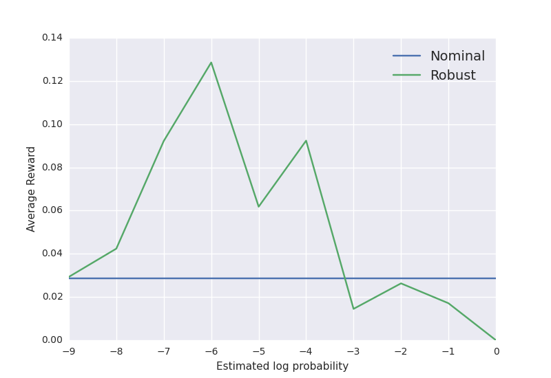
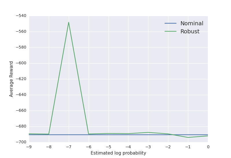
Figure 2: Performance of robust models with different sizes of confidence regions on two environments. Left: FrozenLake-v0 Right: Acrobot-v1

Note that there is a tradeoff in the performance of the robust algorithms versus the nominal algorithms in terms of the value $p$. As the value of $p$ increases, we expect the robust algorithm to gain an edge over the nominal ones as long as $\widehat{U}$ is still within the simplex $\Delta_{n}$. Once we exceed the simplex $\Delta_{n}$ however, the robust algorithms decays in performance. This is due to the presence of the $\beta$ term in the convergence results, which is defined as

$$\beta\coloneqq\max_{i\in\mathcal{X},a\in\mathcal{A}}\max_{y\in\widehat{U^{a}_{i}}}\min_{x\in U^{a}_{i}}\left\|y-x\right\|_{1},$$ (135)

and it grows larger proportional to how much the proxy confidence region $\widehat{U}$ is outside $\Delta_{n}$. Note that while $\beta$ is $0$, the robust algorithms converge to the exact $\operatorname{Q}$-factor and value function, while the nominal algorithm does not. However, since large values of $\beta$ also lead to suboptimal convergence, we also expect poor performance for too large confidence regions, i.e., large values of $p$. Figure 2 depicts how the size of the confidence region affects the performance of the robust models; note that the. Note that the average score appears somewhat erratic as a function of the size of the uncertainty set, however this is due to our small sample size used in the line search. See Figures 3, 4, 5, 6, 7, 8, 9, 10, 11, and 12 for a comparison of the best robust model and the nominal model.

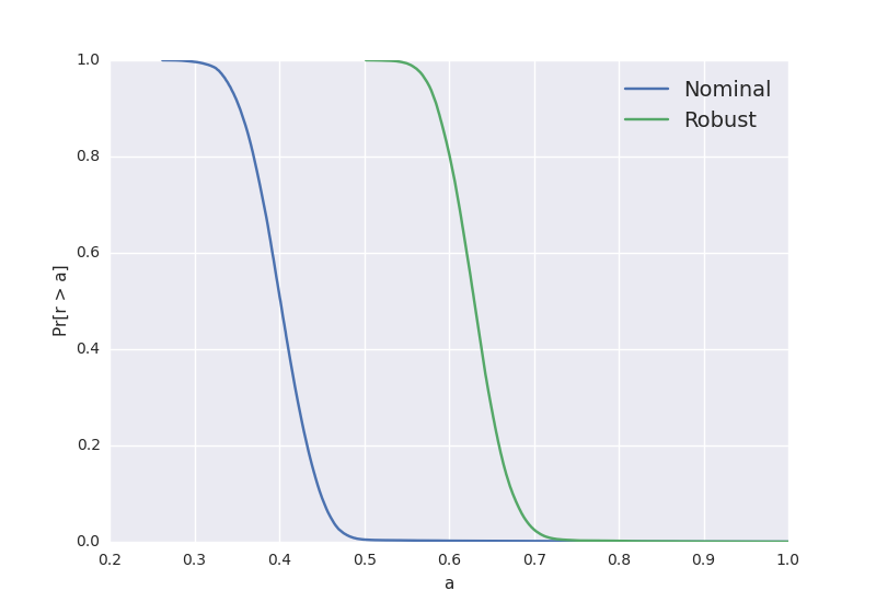
Figure 3: Tail distribution and cumulative rewards during transient and stationary phase of robust vs nominal $\operatorname{Q}$-learning on FrozenLake8x8-v0 with $p=0.01$.

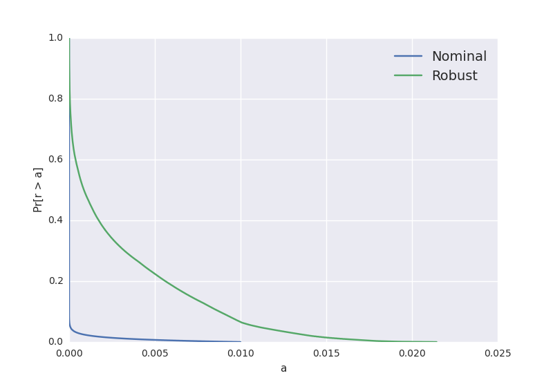
Figure 4: Tail distribution and cumulative rewards during transient and stationary phase of robust vs nominal $\operatorname{Q}$-learning on FrozenLake8x8-v0 with $p=0.1$.

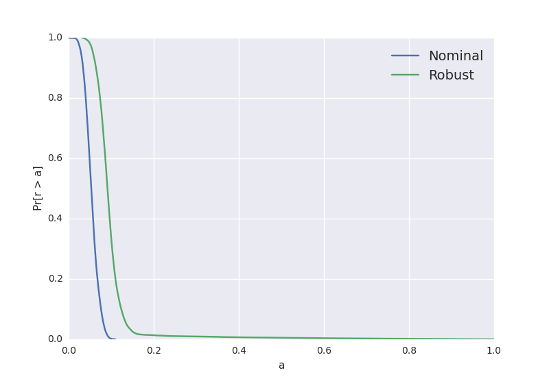
Figure 5: Tail distribution and cumulative rewards during transient and stationary phase of robust vs nominal $\operatorname{Q}$-learning on FrozenLake-v0 with $p=0.1$.

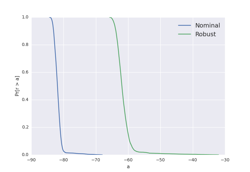
Figure 6: Tail distribution and cumulative rewards during transient and stationary phase of robust vs nominal $\operatorname{Q}$-learning on CartPole-v0 with $p=0.001$.

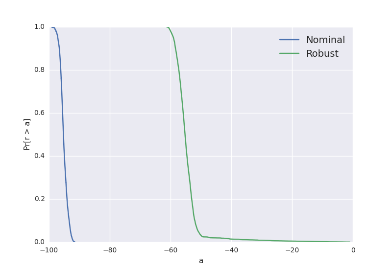
Figure 7: Tail distribution and cumulative rewards during transient and stationary phase of robust vs nominal $\operatorname{Q}$-learning on CartPole-v0 with $p=0.01$.

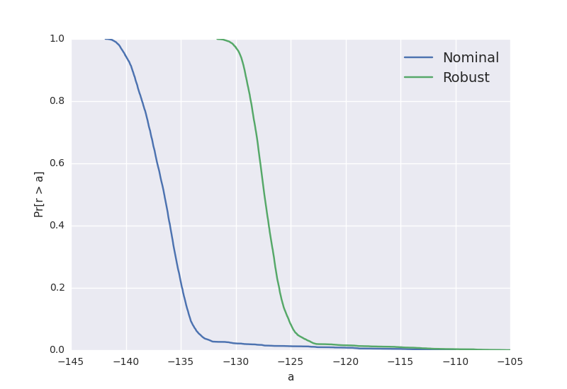
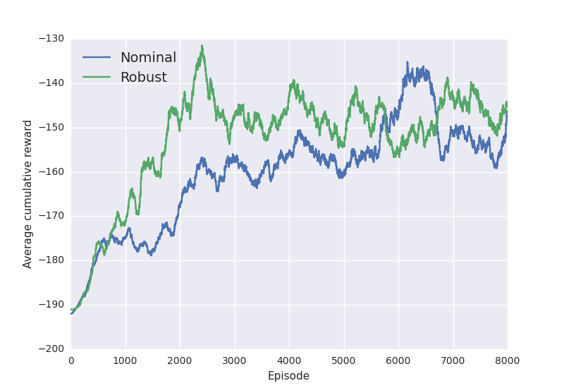
Figure 8: Tail distribution and cumulative rewards during transient and stationary phase of robust vs nominal $\operatorname{Q}$-learning on CartPole-v0 with $p=0.3$.

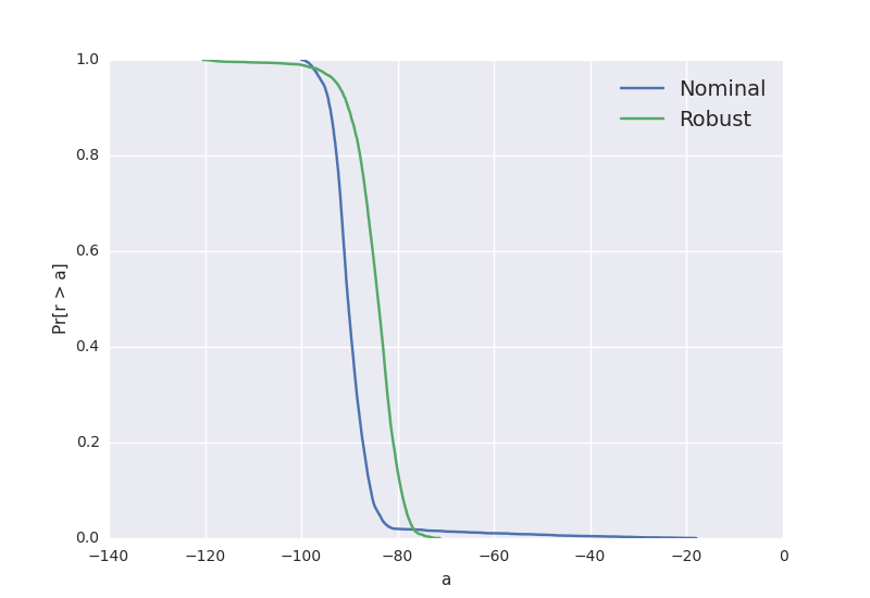
Figure 9: Tail distribution and cumulative rewards during transient and stationary phase of robust vs nominal $\operatorname{Q}$-learning on CartPole-v1 with $p=0.1$.

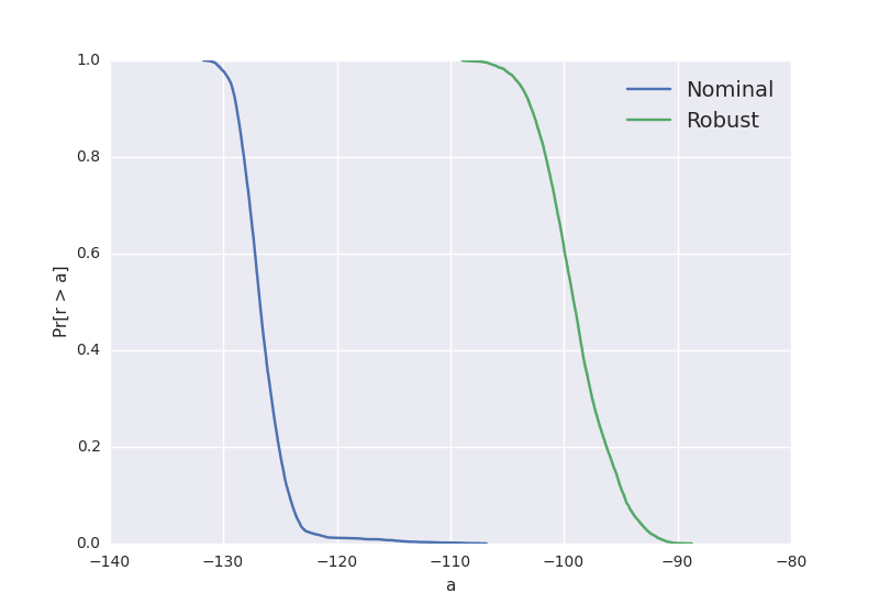
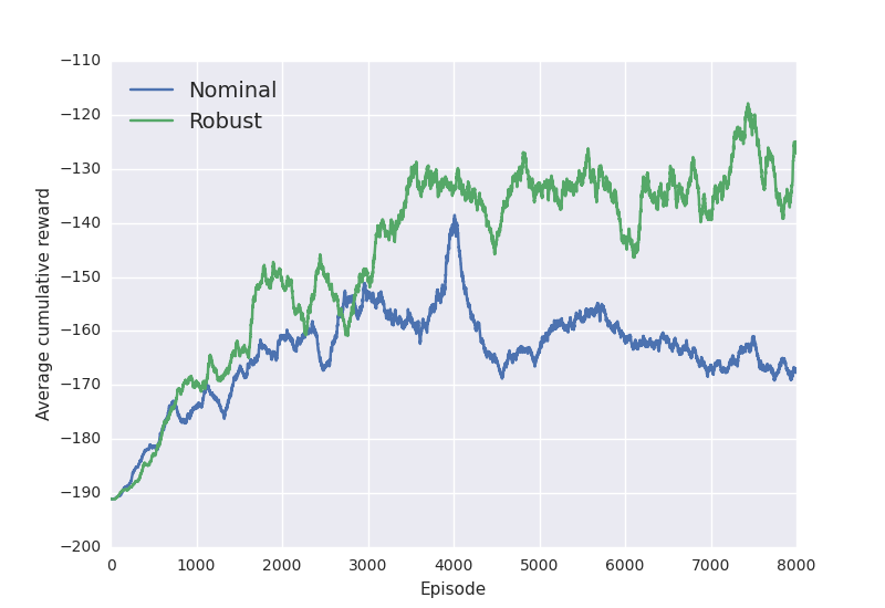
Figure 10: Tail distribution and cumulative rewards during transient and stationary phase of robust vs nominal $\operatorname{Q}$-learning on CartPole-v1 with $p=0.3$.

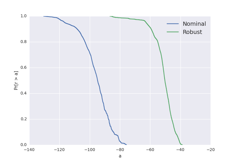
Figure 11: Tail distribution and cumulative rewards during transient and stationary phase of robust vs nominal $\operatorname{Q}$-learning on Taxi-v2 with $p=0.1$.

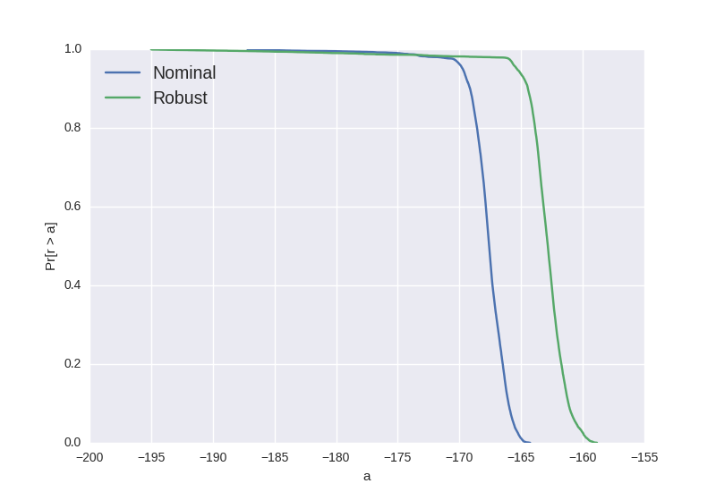
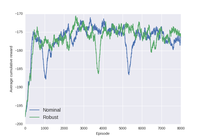
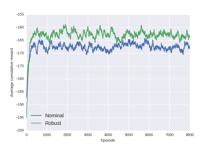
Figure 12: Tail distribution and cumulative rewards during transient and stationary phase of robust vs nominal $\operatorname{Q}$-learning on InvertedPendulum-v1 with $p=0.1$.

6 Acknowledgments

The authors would like to thank Guy Tennenholtz and anonymous reviewers for helping improve the presentation of the paper.

References

- [1] András Antos, Csaba Szepesvári, and Rémi Munos. Learning near-optimal policies with bellman-residual minimization based fitted policy iteration and a single sample path. Machine Learning, 71(1):89–129, 2008.
- [2] J Andrew Bagnell, Andrew Y Ng, and Jeff G Schneider. Solving uncertain markov decision processes. 2001.
- [3] Dimitri P Bertsekas. Approximate policy iteration: A survey and some new methods. Journal of Control Theory and Applications, 9(3):310–335, 2011.
- [4] Dimitri P Bertsekas and Sergey Ioffe. Temporal differences-based policy iteration and applications in neuro-dynamic programming. Lab. for Info. and Decision Systems Report LIDS-P-2349, MIT, Cambridge, MA, 1996.
- [5] Dimitri P Bertsekas and John N Tsitsiklis. Neuro-dynamic programming: an overview. In Decision and Control, 1995., Proceedings of the 34th IEEE Conference on, volume 1, pages 560–564. IEEE, 1995.
- [6] Dimitri P Bertsekas and Huizhen Yu. Projected equation methods for approximate solution of large linear systems. Journal of Computational and Applied Mathematics, 227(1):27–50, 2009.
- [7] Shalabh Bhatnagar, Doina Precup, David Silver, Richard S Sutton, Hamid R Maei, and Csaba Szepesvári. Convergent temporal-difference learning with arbitrary smooth function approximation. In Advances in Neural Information Processing Systems, pages 1204–1212, 2009.
- [8] Justin A Boyan. Technical update: Least-squares temporal difference learning. Machine Learning, 49(2-3):233–246, 2002.
- [9] Steven J Bradtke and Andrew G Barto. Linear least-squares algorithms for temporal difference learning. Machine learning, 22(1-3):33–57, 1996.
- [10] Greg Brockman, Vicki Cheung, Ludwig Pettersson, Jonas Schneider, John Schulman, Jie Tang, and Wojciech Zaremba. Openai gym. arXiv preprint arXiv:1606.01540, 2016.
- [11] Erick Delage and Shie Mannor. Percentile optimization for markov decision processes with parameter uncertainty. Operations research, 58(1):203–213, 2010.
- [12] Amir M Farahmand, Mohammad Ghavamzadeh, Shie Mannor, and Csaba Szepesvári. Regularized policy iteration. In Advances in Neural Information Processing Systems, pages 441–448, 2009.
- [13] Garud N Iyengar. Robust dynamic programming. Mathematics of Operations Research, 30(2):257–280, 2005.
- [14] Shiau Hong Lim, Huan Xu, and Shie Mannor. Reinforcement learning in robust markov decision processes. In Advances in Neural Information Processing Systems, pages 701–709, 2013.
- [15] Jun Morimoto and Kenji Doya. Robust reinforcement learning. Neural computation, 17(2):335–359, 2005.
- [16] A Nedić and Dimitri P Bertsekas. Least squares policy evaluation algorithms with linear function approximation. Discrete Event Dynamic Systems, 13(1):79–110, 2003.
- [17] Arnab Nilim and Laurent El Ghaoui. Robustness in markov decision problems with uncertain transition matrices. In NIPS, pages 839–846, 2003.
- [18] Lerrel Pinto, James Davidson, Rahul Sukthankar, and Abhinav Gupta. Robust adversarial reinforcement learning. arXiv preprint arXiv:1703.02702, 2017.
- [19] Warren B Powell. Approximate Dynamic Programming: Solving the curses of dimensionality, volume 703. John Wiley & Sons, 2007.
- [20] Martin L Puterman. Markov decision processes: discrete stochastic dynamic programming. John Wiley & Sons, 2014.
- [21] Alexander Shapiro and Anton Kleywegt. Minimax analysis of stochastic problems. Optimization Methods and Software, 17(3):523–542, 2002.
- [22] Richard S Sutton and Andrew G Barto. Reinforcement learning: An introduction, volume 1. MIT press Cambridge, 1998.
- [23] Richard S Sutton, Hamid R Maei, and Csaba Szepesvári. A convergent temporal-difference algorithm for off-policy learning with linear function approximation. In Advances in neural information processing systems, pages 1609–1616, 2009.
- [24] Richard S Sutton, Hamid Reza Maei, Doina Precup, Shalabh Bhatnagar, David Silver, Csaba Szepesvári, and Eric Wiewiora. Fast gradient-descent methods for temporal-difference learning with linear function approximation. In Proceedings of the 26th Annual International Conference on Machine Learning, pages 993–1000. ACM, 2009.
- [25] Aviv Tamar, Yonatan Glassner, and Shie Mannor. Optimizing the cvar via sampling. arXiv preprint arXiv:1404.3862, 2014.
- [26] Aviv Tamar, Shie Mannor, and Huan Xu. Scaling up robust mdps using function approximation. In ICML, volume 32, page 2014, 2014.
- [27] Emanuel Todorov, Tom Erez, and Yuval Tassa. Mujoco: A physics engine for model-based control. In Intelligent Robots and Systems (IROS), 2012 IEEE/RSJ International Conference on, pages 5026–5033. IEEE, 2012.
- [28] Wolfram Wiesemann, Daniel Kuhn, and Berç Rustem. Robust markov decision processes. Mathematics of Operations Research, 38(1):153–183, 2013.