A softening-healing law for self-healing quasi-brittle materials: analyzing with Strong Discontinuity embedded Approach

Abstract

Quasi-brittle materials such as concrete suffer from cracks during their life cycle, requiring great cost for conventional maintenance or replacement. In the last decades, self-healing materials are developed which are capable of filling and healing the cracks and regaining part of the stiffness and strength automatically after getting damaged, bringing the possibility of maintenance-free materials and structures.

In this paper, a time dependent softening-healing law for self-healing quasi-brittle materials is presented by introducing limited material parameters with clear physical background. Strong Discontinuity embedded Approach (SDA) is adopted for evaluating the reliability of the model. In the numerical studies, values of healing parameters are firstly obtained by back analysis of experimental results of self-healing beams. Then numerical models regarding concrete members and structures built with self-healing and non-healing materials are simulated and compared for showing the capability of the self-healing material.

1 Introduction

In engineering practices, the damage of quasi-brittle materials such as concrete, glass and ceramic manifests itself in the form of micro and macro cracks, jeopardizing the serviceability and durability of the structures and resulting into considerable maintenance and repair costs [1]. Self-healing quasi-brittle materials attracted great interests in these years, which are capable of filling and repairing the cracks automatically, making it possible to greatly save the life term costs even build maintenance-free structures [2].

The author of [3] produced the first self-healing cement in 1990s. After then, different self-healing strategies for quasi-brittle materials, especially for cementitious materials are presented, mainly including

• implementations of hollow fibers or micro capsules carrying bonding medium such as resin or component promoting chemical reaction of original material such as water for high strength concrete [4, 5, 6, 7, 8];

• utilizing bacteria for promoting the precipitation of calcium carbonate, which are commonly carried by micro capsules [9, 10, 11, 12, 13];

• using shape memory materials for providing traction between and closing the cracks [14, 15, 16, 17];

with detailed discussions and comparisons provided in [18, 19, 20, 21, 22, 23]. In these strategies, there are not enough results about the mechanical recovery regarding the bacteria healing method, although it has been proved to be very effective for controlling the long term mass transport e.g. permeation and diffusion inside crack opening. On the other hand, the other two methods refer to conspicuous recovery of mechanical properties of the damage material as shown in experimental investigations.

For numerically simulating the damage-healing behavior, based on Continuum Damage Mechanics (CDM), a consistent thermodynamic framework coined Continuum Damage-Healing Mechanics (CDHM) was firstly presented in [24], which considered healing as a kind of “negative damage” and presented a general framework for describing the degradation-healing of composites. Belong to the family of CDHM, more recent methods are presented in these years [25, 26, 27, 28, 29] including a version coined Cohesive Zone Damage-Healing model [30, 31]. Based on CDHM, in [32] Fracture Process Zone (FPZ) elements and Shape Memory Polymer (SMP) tendon elements are respectively built and prescribed at the damage domain of the self-healing beam, for predicting the long-term mechanical behaviour of SMP reinforced concrete beam, as a recent engineering application. CDHM was built based on CDM and inherits the basic assumptions of the latter, which introduces internal state variables and considers the damage-healing as reduction-increasing of stiffness and strength. And the corresponding constitutive relationship is commonly built for strain and stress.

During damage of quasi-brittle materials, micro-defects merge into macro-cracks and the size of fracture zone reduces from finite width to almost zero in a very limited loading period, the behavior of which is localized and anisotropic, highly depending on the crack locations and orientations [33, 34]. From this point of view, discontinuous models such as conventional interface element [35, 36, 37, 38, 39], Strong Discontinuity embedded Approach (SDA or E-FEM) and localization [40, 41, 42, 43, 44, 45, 46, 47, 48, 49], nodal enrichment method eXtended Finite Element Method (X-FEM) [50, 51, 52, 53, 54, 55, 56, 57] and phantom node method [58, 59, 60] could be more suitable for especially simulating the damage process of quasi-brittle materials, which holds much less mesh dependence than continuous method. Correspondingly, when using discontinuous models for self-healing quasi-brittle materials, as a pseudo reverse damage process, healing should also be considered in a discontinuous form e.g. in the form of traction-separation law [61] for describing the relationship between crack opening and traction inside the cracks instead of strain and stress.

In this paper, we present a softening-healing law in the form of traction-separation which is naturally compatible with discontinuous numerical models for quasi-brittle materials. The law is built based on simple assumptions and only a few healing parameters with physical background are introduced. The factors of trigger and maturity of the healing process, despite of other forms of stimuli in practices such as optical [62] and electrical [63], are assumed to be crack opening and time respectively. An SDA presented by us before in [64] is taken as the numerical framework for testing the softening-healing law, which of course does not restrict the implementation of the law in other numerical models. Through back analysis regarding experimental results of a loading-reloading test of a self-healing concrete beam, the range of the healing parameters are determined. Structure such as concrete member and gravity dam model are simulated for showing the advantage by using self-healing materials in engineering practices.

The remaining parts of the paper is organized as in Section 2, the proposed softening-healing law is presented, by assuming the traction-separation law of self-healing material depends on the properties of the healing agent as well as the original quasi-brittle material, then the formulation of SDA in our published literature as the numerical framework is briefly introduced. In Section 3, the range of the material parameters of the self-healing material are determined by back analysis of loading-reloading bending tests of self-healing concrete beams. Then, a tension-shear test is numerically analyzed for evaluating the healing efficiency of healing agent at different loading stage. Finally a gravity dam model is simulated for showing the different working behaviors of the engineering structures built with self-healing and non-healing materials. This paper closes with concluding remarks given in Section 4.

2 Model

2.1 A softening-healing law

The relationship of the crack opening and the traction between two surface of the crack is built based on a mixed-mode traction-separation [65, 54] law. In 2D conditions, the crack opening is defined as

$$\zeta=\sqrt{\zeta_{n}^{2}+\beta^{2}\zeta_{t}^{2}},$$ (1)

with $\beta$ governing the contribution of Mode I and Mode II crack opening. According to [66, 67], $\beta=1$ is well-suited for quasi-brittle materials such as concrete, which will be considered throughout this paper. $\zeta_{n}$ and $\zeta_{t}$ are the crack opening or crack width along normal and parallel directions of the crack path, with corresponding unit vector denoted as $\mathbf{n}$ and $\mathbf{t}$.

Meanwhile, the traction components along $\mathbf{n}$ and $\mathbf{t}$, $T_{n}$ and $T_{t}$ are obtained as

$$T_{n}=T\frac{\zeta_{n}}{\zeta},~{}T_{t}=T\frac{\zeta_{t}}{\zeta}$$ (2)

with

$$T\left(\zeta\right)=\left\{\begin{array}[]{ll}TL\left(\zeta\right)=f_{t}\ \mbox{exp}\left(-\cfrac{f_{t}}{G_{f}}\zeta\right),&\mbox{loading},\\ TU\left(\zeta\right)=\cfrac{T_{mx}}{\zeta_{mx}}\zeta,&\mbox{unloading/reloading},\end{array}\right.$$

where $f_{t}$ is the uniaxial tensile strength and $G_{f}$ is the fracture energy, $\zeta_{mx}$ is the maximum crack opening the crack ever experienced, and $T_{mx}=TL\left(\zeta_{mx}\right)$ is the corresponding traction, as illustrated in Figure 1.

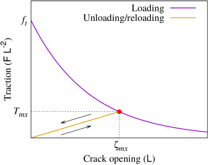
Figure 1: Original traction-seperation law

Regarding a crack which firstly experienced a big crack opening and became almost traction free i.e. $T_{mx}\approx 0$ then was healed by healing agent, when this crack is reopened, the new traction denoted as $H$ is attributed to the healing agent, which depends on $\zeta$ and resting time for healing $\Delta t=t-t_{r}$, with $t_{r}$ being the time when healing agent released. If $\Delta t$ is big enough that the healing agent become completely mature, by mimicking the traction-separation law of the original quasi-brittle material, the new traction-separation law of the healed material is obtained as:

$$H_{\infty}\left(\zeta\right)=\left\{\begin{array}[]{ll}HL_{\infty}\left(\zeta\right)=f_{h,\infty}\ \mbox{exp}\left(-\cfrac{f_{h,\infty}}{G_{h,\infty}}\zeta\right),&\mbox{loading of healed material},\\ HU_{\infty}\left(\zeta\right)=\cfrac{H_{hx}}{\zeta_{hx}}\zeta,&\mbox{unloading/reloading of healed material},\end{array}\right.$$ (3)

where $f_{h,\infty}$ is the ultimate strength and $G_{h,\infty}$ is the ultimate fracture energy of the healed material which was completely damaged before healed. $\zeta_{hx}$ is the maximum crack opening which the crack ever experienced after healing with $\zeta_{hx}\leq\zeta_{mx}$, and $H_{hx}=HL_{\infty}\left(\zeta_{hx}\right)$ is the corresponding traction of healed material. Here, it is worth to emphasize that $f_{h,\infty}$ and $G_{h,\infty}$ depend not only on the material properties of the healing agent but also on the binding properties between the healing agent and the original material. Of course, we would like to mention here that choosing exponential relation in Equations 2 and 3 is only an option, bilinear and hyperbolic curves are also available [68, 69], which could be more appropriate for specific materials or healing agents.

Considering the time-dependent healing behaviour that the strength of healing agent depends on the mature level of healing agent i.e. healing degree $R$ as

$$H\left(\zeta,\Delta t\right)=R\left(\Delta t\right)\ H_{\infty}\left(\zeta\right).$$ (4)

When assuming the solidification of healing agent is a type of chemical reaction similar to the hydration process of cementitious materials [70, 71, 72, 73], an Arrhenius-type law is appropriate for describing $\dot{R}$, indicating $\dot{R}$ depends on temperature and is proportional to the chemical affinity $\tilde{A}$ of healing agent. Furthermore, linear increasing of $f_{h}\left(\Delta t\right)$ and $G_{h}\left(\Delta t\right)$ with healing degree is also assumed, similar to the hydration process of early-age concrete [74, 75]. Because the experimental results of $\tilde{A}$ of cementitious materials are commonly fitted with exponential function, in isothermal condition following function for $R\left(\Delta t\right)$ is assumed

$$R\left(\Delta t\right)=1-\mbox{exp}\left(-A_{h}\ \Delta t\right)=\frac{f_{h}\left(\Delta t\right)}{f_{h,\infty}}=\frac{G_{h}\left(\Delta t\right)}{G_{h,\infty}},$$ (5)

in which $A_{h}$ is the healing speed coefficient.

Herein, the traction-separation law of healing agent within traction free crack is proposed. For the cases with $T_{mx}>0$ which cannot be ignored, the system is considered as a parallel springs system that the equivalent traction $T_{eq}$ is obtained as

$$T_{n}=T_{eq}\frac{\zeta_{n}}{\zeta},~{}T_{t}=T_{eq}\frac{\zeta_{t}}{\zeta}$$ (6)

with

$$T_{eq}\left(\zeta,\Delta t\right)=T\left(\zeta\right)+\alpha\ H\left(\zeta,\Delta t\right)$$

where $\alpha$ is introduced for accounting the level of penetration and contact between the healing agent and the original material inside cohesive crack. It is obvious that $\alpha$ is 0 when $\zeta_{mx}=0$ and will become 1 when $T_{mx}\approx 0$, leading into the following assumed function

$$\left\{\begin{array}[]{ll}\alpha=0,&T_{mx}>T_{0}\\ \alpha=1-\left(T_{mx,r}\ /\ f_{t}\right)^{b},&T_{mx}\leq T_{0}\end{array}\right.$$ (7)

in which, $T_{0}$ is a threshold value of traction indicating the break of carrier (glass tubes or capsules) of healing agents followed by the release and penetration of healing agent into the cohesive crack. $T_{mx,r}$ is the value of $T_{mx}$ at $t_{r}$, as the crack opening when the healing agent was released. $b$ is a coefficient indicating the contact between healing agent and the original material, with a higher value of $b$ indicating better contact, see Figure 2. It can be found that $T_{0}$ indicates the sensitivity of the self-healing capsule to sense damage. If $T_{0}$ is a big value (good sensitivity) when $b$ is a small value (bad contact and penetration), then the healing agent is released but will not perform very well since the crack opening could be a small value. Hence, it is very important to firstly increase the value of $b$ of the healing agent in engineering practices.

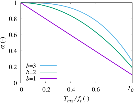
Figure 2: change of $\alpha$ with $T_{mx,r}\ /\ f_{t}$ regarding different values of $b$

Figure 3 illustrates the shapes of $T\left({\zeta}\right)$, $H\left({\zeta}\right)$ and $T_{eq}\left({\zeta}\right)$, showing three parts in $T_{eq}$

• Part I: Both healing agent and original material are under unloading/reloading condition,

• Part II: Healing agent is under loading while original material is under reloading,

• Part III: Both healing agent and original material are under loading.

For better understanding, the new material parameters referring to healing are listed again in Table 1. It can be seen that the presented softening-healing law only introduce limited material parameters, which could be determined through experimental investigations. Besides, since only the material law is changed, the new law could be very easily implemented into the current numerical models for damage analysis of quasi-brittle materials. In the numerical studies provided in Section 3, we will focus on $f_{h,\infty}$ and $G_{h,\infty}$ the range of which are determined with back analysis of experimental results, when the other parameters are mainly assumed.

Table 1: New material parameters referring to healing

Symbol	Unit	Presented in	For denoting
$f_{h,\infty}$	[MPa]	Equation 3	The ultimate tensile strength of mature healing material
$G_{h,\infty}$	[N m-1]	Equation 3	The ultimate fracture energy of mature healed material
$A_{h}$	[h-1]	Equation 5	The healing speed coefficient of healing agent
$T_{0}$	[MPa]	Equation 7	The threshold value of traction triggering the release of healing agent
$b$	[–]	Equation 7	The coefficient indicating the penetration and contact property of the healing agent in the cohesive crack

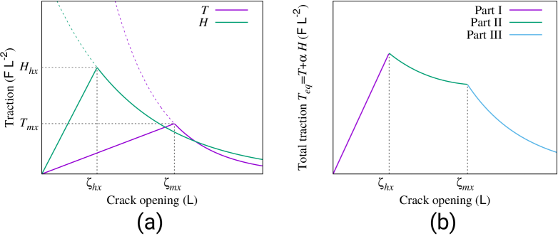
Figure 3: (a) shapes of $T\left({\zeta}\right)$, $H\left({\zeta}\right)$, (b) shape of $T_{eq}\left({\zeta}\right)$

2.2 Strong Discontinuity embedded Approach (SDA)

The Strong Discontinuity embedded Approach (SDA) adopted in this paper is built based on standard Statically Optimal Symmetric (SOS) formulation [76, 77, 78]. Recently in [64], we have proven when implemented into quadrilateral 8 node element with quadratic interpolation of the displacement field (Q8), the presented SDA model shows no stress locking as well as almost no mesh bias, which is also simple for coding and holds good numerical stability regarding standard Galerkin method. The SDA model is briefly described as follows, when more detailed descriptions were given in [64, 79, 80, 81].

Regarding a 2D domain $\Omega$ separated by a discontinuity $\mathbf{L}$ into $\Omega^{+}$ and $\Omega^{-}$ with normal and parallel unit vector $\mathbf{n}$ and $\mathbf{t}$, a localized subdomain $\Omega_{\varphi}$ is introduced for avoiding singularity, leading to the displacement field of $\Omega$

$$\mathbf{u}(\mathbf{x})=\bar{\mathbf{u}}(\mathbf{x})+[H_{s}(\mathbf{x})-\varphi(\mathbf{x})]\llbracket u\rrbracket,$$ (8)

where $\bar{\mathbf{u}}(\mathbf{x})$ is the regular part, $H_{s}(\mathbf{x})$ is the Heaviside function, and $\varphi(\mathbf{x})$ is a smooth derivable function with $\varphi(\mathbf{x})\in\left[0,1\right]$, see Figure 4.

Figure 4: Domain $\Omega$ and its displacement field

The strain field [82] is correspondingly obtained as

$$\begin{array}[]{cccc}\boldsymbol{\varepsilon}(\mathbf{x})=\nabla^{S}\mathbf{u}(\mathbf{x})=&\underbrace{\nabla^{S}\bar{\mathbf{u}}(\mathbf{x})-(\llbracket u\rrbracket(\mathbf{x})\otimes\nabla\varphi)^{S}}&+&\underbrace{\delta_{\mathbf{L}}(\llbracket u\rrbracket(\mathbf{x})\otimes\mathbf{n})^{S}},\\ &\bar{\boldsymbol{\varepsilon}}(\mathbf{x}),\forall x\in\Omega\setminus\mathbf{L}&&{\boldsymbol{\varepsilon}}_{\delta}(\mathbf{x}),\forall x\in\mathbf{L}\end{array}$$ (9)

where $(\cdot)^{S}$ denotes the symmetric part of the tensor and $\delta_{\mathbf{L}}$ stands for the Dirac-delta distribution. After assuming $\nabla\llbracket u\rrbracket(\mathbf{x})=0$ and further decomposing $\llbracket u\rrbracket(\mathbf{x})=\zeta_{n}(\mathbf{x})\mathbf{n}+\zeta_{t}(\mathbf{x})\mathbf{t}$, compatible strains and enhanced strains [83] are obtained as

$$\begin{array}[]{cccc}\bar{\boldsymbol{\varepsilon}}(\mathbf{x})=&\underbrace{\nabla^{S}\bar{\mathbf{u}}(\mathbf{x})}&-&\underbrace{\left[(\mathbf{n}\otimes\nabla\varphi)^{S}\zeta_{n}(\mathbf{x})+(\mathbf{t}\otimes\nabla\varphi)^{S}\zeta_{t}(\mathbf{x})\right]},\\ &\mbox{total strain }\boldsymbol{\varepsilon}^{t}&&\mbox{enhanced strain }\widetilde{\boldsymbol{\varepsilon}}\end{array}$$ (10)

Based on SOS formulation and the conservation of dissipated energy in localized element and using reduced integration scheme, in [64] we obtained $\nabla\varphi=\mathbf{n}\ /\ l_{c}$ and $l_{c}=V\ /\ A$, where $V$ is the volume of the element and $A$ is the area of a parallel crack passing through center point, see Figure 5, and $l_{c}$ corresponds to the classical characteristic length [84], which only depends on the shape of the local element. Once the crack direction is determined by the so called crack tracking strategy [85, 86, 87, 88, 89, 90], $l_{c}$ is directly obtained. Hence, in the local element “$e$”, following relationship is obtained

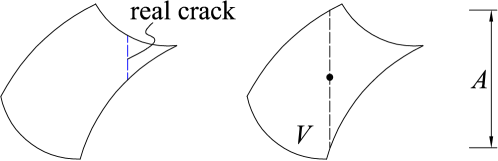
Figure 5: Determinating the effective cracking area $A$

$$\bar{\boldsymbol{\varepsilon}}^{(e)}(\mathbf{x})\approx\sum^{n_{e}}_{i=1}\left(\nabla N^{(e)}_{i}\otimes\mathbf{u}_{i}\right)^{S}-\frac{1}{\ l_{c}\ }\left[(\mathbf{n}\otimes{\mathbf{n}})\zeta_{n}^{(e)}+(\mathbf{n}\otimes{\mathbf{t}})^{S}\zeta^{(e)}_{t}\right],$$ (11)

where ${n_{e}}$ is the number of nodes of element ”$e$”, $N^{(e)}$ is the shape function, and $\mathbf{u}_{i}$ is the displacement vector of node ”$i$”.

2.3 Algorithmic formulation

Regarding the states at steps “$i-1$” and “$i$”, extra subscript is used for showing different parameters in these two steps, for example $\zeta_{i}$ is the crack opening at step $i$. Hereby, the states at “$i-1$” are all known when most states at “$i$” are unknown. At step “$i$”, the trial stress state is obtained as

$$\boldsymbol{\sigma}^{tr}_{i}=\mathbb{C}:\left\{\boldsymbol{\varepsilon}^{t}_{i}-\frac{1}{\ l_{c}\ }\left[(\mathbf{n}\otimes\mathbf{n})\zeta_{n,i-1}+(\mathbf{n}\otimes\mathbf{t})^{S}\zeta_{t,i-1}\right]\right\},$$ (12)

where $\mathbb{C}$ is the elasticity tensor. Regarding the balance relation, the unknown incremental state variables $\Delta\zeta_{n,i}=\zeta_{n,i}-\zeta_{n,i-1}$ and $\Delta\zeta_{t,i}=\zeta_{t,i}-\zeta_{t,i-1}$ are determined from

$$\left[\begin{array}[]{c}\mathbf{V}_{1}\\ \mathbf{V}_{2}\end{array}\right]:\boldsymbol{\sigma}^{tr}_{i}-\frac{1}{\ l_{c}\ }\left[\begin{array}[]{cc}\mathbf{V}_{1}:\mathbb{C}:\mathbf{V}_{1}&\mathbf{V}_{1}:\mathbb{C}:\mathbf{V}_{2}\\ \mathbf{V}_{2}:\mathbb{C}:\mathbf{V}_{1}&\mathbf{V}_{2}:\mathbb{C}:\mathbf{V}_{2}\end{array}\right]\left[\begin{array}[]{c}\Delta\zeta_{n,i}\\ \Delta\zeta_{t,i}\end{array}\right]-\left[\begin{array}[]{c}T_{n}\\ T_{t}\end{array}\right]=\mathbf{0}$$ (13)

with $\mathbf{V}_{1}=(\mathbf{n}\otimes\mathbf{n})$ and $\mathbf{V}_{2}=(\mathbf{n}\otimes\mathbf{t})^{S}$.

Regarding infinitesimal multisurface plasticity [91, 92, 93], the corresponding elastoplastic tangent moduli $\mathbb{C}^{ep}$ at step $i$ is

$$\mathbb{C}^{ep}=\frac{d\boldsymbol{\sigma}_{i}}{d\boldsymbol{\varepsilon}^{t}_{i}}=\mathbb{C}-\mathbb{S},$$ (14)

where

$$\mathbb{S}=\mathbb{C}:\left[\begin{array}[]{cc}\mathbf{V}_{1}&\mathbf{V}_{2}\\ \end{array}\right]:\left(\mathbf{G}+l_{c}\ \mathbf{D}\right)^{-1}:\left[\begin{array}[]{c}\mathbf{V}_{1}\\ \mathbf{V}_{2}\end{array}\right]:\mathbb{C}$$ (15)

with

$$\mathbf{G}=\left[\begin{array}[]{cc}\mathbf{V}_{1}:\mathbb{C}:\mathbf{V}_{1}&\mathbf{V}_{1}:\mathbb{C}:\mathbf{V}_{2}\\ \mathbf{V}_{2}:\mathbb{C}:\mathbf{V}_{1}&\mathbf{V}_{2}:\mathbb{C}:\mathbf{V}_{2}\end{array}\right],$$

and

$$\mathbf{D}=\mathbf{D}_{o}+\alpha\ \mathbf{D}_{h}$$ (16)

where

$$\begin{array}[]{l}\mathbf{D}_{o}=-\frac{T}{\zeta}\left[\begin{array}[]{cc}\frac{\zeta_{n}^{2}}{\zeta^{2}}+\frac{f_{t}\zeta_{n}^{2}}{G_{f}\zeta}-1&\frac{\zeta_{n}\zeta_{t}}{\zeta^{2}}+\frac{f_{t}\zeta_{n}\zeta_{t}}{G_{f}\zeta}\\ \frac{\zeta_{n}\zeta_{t}}{\zeta^{2}}+\frac{f_{t}\zeta_{n}\zeta_{t}}{G_{f}\zeta}&\frac{\zeta_{t}^{2}}{\zeta^{2}}+\frac{f_{t}\zeta_{t}^{2}}{G_{f}\zeta}-1\\ \end{array}\right]\mbox{ for loading of original material},\\ \mbox{and}\\ \mathbf{D}_{o}=\frac{T_{mx}}{\zeta_{mx}}\left[\begin{array}[]{cc}1&0\\ 0&1\end{array}\right]\mbox{ for unloading/reloading of original material},\end{array}$$ (17)

and

$$\begin{array}[]{l}\mathbf{D}_{h}=-\frac{H}{\zeta}\left[\begin{array}[]{cc}\frac{\zeta_{n}^{2}}{\zeta^{2}}+\frac{f_{h,\infty}\zeta_{n}^{2}}{G_{h,\infty}\zeta}-1&\frac{\zeta_{n}\zeta_{t}}{\zeta^{2}}+\frac{f_{h,\infty}\zeta_{n}\zeta_{t}}{G_{h,\infty}\zeta}\\ \frac{\zeta_{n}\zeta_{t}}{\zeta^{2}}+\frac{f_{h,\infty}\zeta_{n}\zeta_{t}}{G_{h,\infty}\zeta}&\frac{\zeta_{t}^{2}}{\zeta^{2}}+\frac{f_{h,\infty}\zeta_{t}^{2}}{G_{h,\infty}\zeta}-1\\ \end{array}\right]\mbox{ for loading of healing agent},\\ \mbox{and}\\ \mathbf{D}_{h}=\frac{H_{hx}}{\zeta_{hx}}\left[\begin{array}[]{cc}1&0\\ 0&1\end{array}\right]\mbox{ for unloading/reloading of healing agent}.\end{array}$$ (18)

3 Numerical analysis

3.1 Bending test for back analysis

For determining the material parameters of healing agent, the results of three point bending test of a self-healing concrete beam provided in [94] are taken. The set-up of the test and material parameters of concrete is shown in Figure 6 [94, 95], with a mixture ratio of concrete as water/cement/sand/gravel = 1/2/4.47/8.53. The material properties of the concrete were not directly provided in [94], but taken by us based on other fracture tests with similar concrete mixture in [96, 97]. Glass capsules filled with two-component expansive polyurethane-based healing agent are casted inside the concrete beam. The simple supported beam was vertically loaded in the middle with a displacement speed 0.04 mm/min, considered as static loading condition. The force $F$ and Crack Mouth Opening Displacement (CMOD) of the notch were recorded. The beam was firstly loaded until CMOD reached 0.3 mm, which was completely unloaded and stored for 24 hours. Thereafter the loading procedure was repeated for assessing the performance of healing. Considering the loading condition, $t_{r}$ is taken as the time when CMOD=0.3 mm was firstly reached.

Figure 6: Set-up of the bending test and material properties of concrete

In this test, the crack tracking strategy is not used. Firstly a straight crack path is prescribed, regarding three different discretization. The force-CMOD curves shown in Figure 8 indicate the adopted SDA model providing results with no mesh bias, as before pointed out in [64]. Hence, in the following analysis, only Mesh I is used. Furthermore, when in reality the crack path is commonly not a straight line as prescribed, curved crack paths described by equation $\sqrt{y}+a\left(x-x_{0}\right)=0$ with $a$ and $x_{0}$ as parameters are also taken into account, the obtained force-CMOD curves of which are shown in Figure 9 (case with straight path denoted as C0). In the back analysis of the healing-reloading test, curved paths are considered together with the straight crack path.

As mentioned before, we will mainly focus on $f_{h,\infty}$ and $G_{h,\infty}$ in this section. When assuming the healing degree of the healing agent reached 90% after 24 hours resting, as $A_{h}=0.096\ \mbox{h}^{-1}$, the evolution of healing agent is shown in Figure 4. Further by taking $b=2.0$ and $T_{0}=0.5\ f_{t}$, $f_{h,\infty}=0.7\ \mbox{MPa}$ and $G_{h,\infty}=42\ \mbox{N/m}$ are obtained from the back analysis. The numerically-obtained force $F_{RE}$-CMOD curves of reloading are shown in Figure 10, indicating acceptable agreements between numerically and experimental-obtained results.

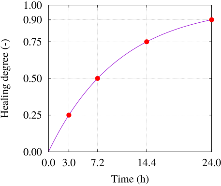
Figure 7: Assumed evolution of maturity of the healing agent based on Equation 5

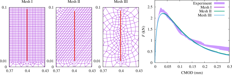
Figure 8: Force-CMOD curves of the bending test, considering different discretizations

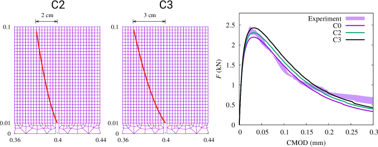
Figure 9: Force-CMOD curves of the bending test (case with straight path denoted as C0), considering curved crack paths (curve equation $\sqrt{y}+a\left(x-x_{0}\right)=0$)

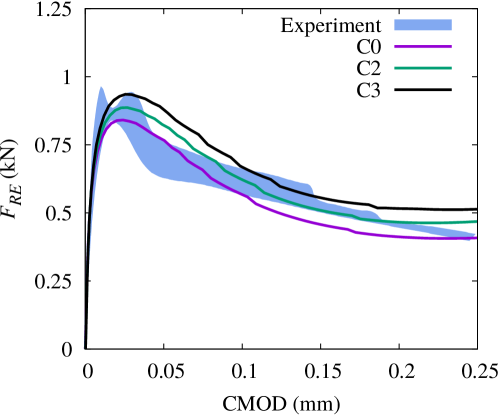
Figure 10: Force-CMOD curves of the reloading test after healing, considering straight and curved crack paths

3.2 Tension-shear test

The second example is the tension-shear test [98]. The model, loading and support conditions are shown in Figure 11, with the ”Load Path 4” in [98] and horizontal load $F_{s}=10$kN considered. First, $F_{s}$ is applied and kept constant. Thereafter, $F_{n}$ is gradually increased, leading to a vertical displacement $d$ and to cracking of the structure. The energy-based crack tracking strategy [64] is used for predicting the crack propagations. The original crack paths and the load-displacement curves of non-healing material are shown in Figure 12, with the comparisons with experimental results [98] and numerical results obtained by the XFEM [54].

Regarding the self-healing parameters, $f_{h,\infty}=0.7\ \mbox{MPa}$ and $G_{h,\infty}=50\ \mbox{N/m}$ are taken, similar to the values obtained from the back analysis. Meanwhile, $A_{h}=0.096\ \mbox{h}^{-1}$, $b=2.0$ and $T_{0}=0.5\ f_{t}$ are assumed. Three reloading cases with target $d$=0.04 mm, 0.06 mm and 0.08 mm are considered. Firstly the structure is loaded till the targeted $d$ is reached when $t_{r}$ is taken as the corresponding time, then $F_{n}$ is reduced to zero and begins to increase again after 24 hours, in the whole procedure of which $F_{s}$ keeps as 10 kN. The Load-displacement curves are shown in Figure 13, indicating that the recovery of mechanical strength was captured by the presented softening-healing model. On the other hand, it could be found when using the model, the contraction is obtained even when the structure is not fully unloaded, which was not completely proven in experimental investigations. More studies will be carried on in the future. On the other hand, the influence of healing on the further propagated crack path is also evaluated. Figure 14 shows the different crack path of the cases with and without healing, indicating the healing process slightly reduces the curvature of the crack path. Nevertheless, we would like to mention that this difference can be almost ignored in this case.

Figure 11: Geometric properties, material parameters, and support conditions of tension-shear test

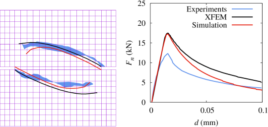
Figure 12: Original crack paths and load-displacement curves of tension-shear test, compared with experimental results [98] and numerical results obtained by the XFEM [54]

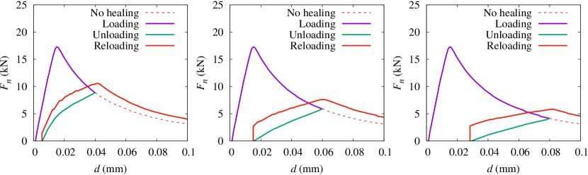
Figure 13: Load-displacement curves of tension-shear test when firstly unloaded at $d$=0.04 mm, 0.06 mm and 0.08 mm, then healed and reloaded after 24h

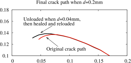
Figure 14: Influence of healing on the further propagated crack path

3.3 A gravity dam model

Hydraulic structures such as dams are very suitable for using self-healing materials, when these structures are commonly

• designed and constructed for over decades of long term working,

• suffered from initial imperfection such as shrinkage cracking of early-age concrete and durability problems such as leakage,

• in large scale and partially under water, which are expensive for traditional maintaining and repairing involving human effort.

Hence, we simulate the gravity dam model experimentally investigated in [99] for illustrating the advantages by using self-healing materials regarding the mechanical behavior. The model was shown in Figure 15, with the notch considered as a kind of imperfection of the original structure which could be healed by using self-healing materials. Similar to the experimental set-up, in the numerical model, the load was simplified by concentrated forces at 4 heights. The arc-length method is used for inducing a constant increment for the CMOD of the notch. The obtained force-CMOD curves and crack paths of non-healing are shown in Figure 16, comparing to the numerical results in [37, 100].

In the numerical analysis with self-healing material, we consider CMOD=0.075 is the initial step for loading and keep a constant increment $\Delta\mbox{CMOD}=0.025$mm. The time for every increment is $\Delta t$, as shown in Figure 17. Furthermore, an explicit strategy is used for obtaining $t_{r}$, that if the crack further propagates between calculation step $i-1$ and $i$, from position $\mathbf{x}_{i-1}$ to $\mathbf{x}_{i}$ with corresponding time $t_{i-1}$ and $t_{i}$ and $T_{mx}\leq T_{0}$, then $t_{r}=t_{i}$ is considered for the crack $\mathbf{x}_{i-1}\rightarrow\mathbf{x}_{i}$. A sensitive healing agent with good penetration property is assumed, with $T_{0}=0.9\ f_{t}$ and $b=3.0$. Considering $\Delta t$=3.0 h and $\Delta t$=7.2 h, the load-CMOD curves of the self-healing structures are show in Figure 18, indicating dam model with self-healing material holds better bearing capacity and post peak behavior, even when $\Delta t$=3.0 h.

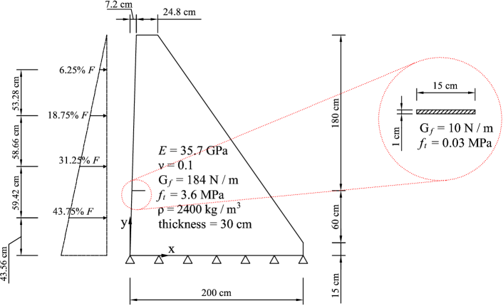
Figure 15: Geometric properties, material parameters, and support conditions of the gravity dam model

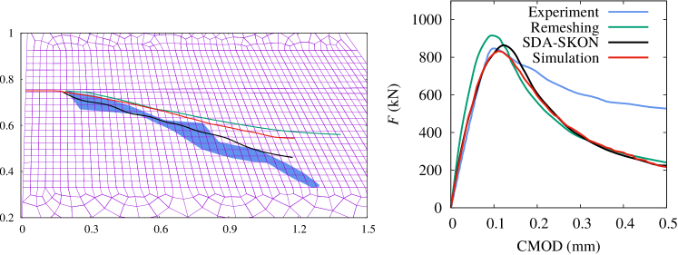
Figure 16: Original load-CMOD curves and crack paths of the dam model, compared with experimental results [99] and numerical results obtained by remeshing [37] and strain injection (upgraded SDA-SKON) [100] methods

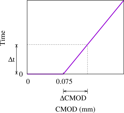
Figure 17: The loading step used in the dam model

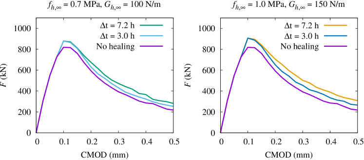
Figure 18: Load-CMOD curves of the dam model with self-healing materials

4 Conclusions

In this paper, aiming at the traction-separation property of the self-healing quasi-brittle materials, we present a softening-healing law. The law is built based on simple assumptions with limited material parameters introduced. The new parameters take into account the properties of maturity, strength, trigger effect, contact and penetration with the original material of the healing agent. A strong discontinuity embedded approach presented by us before is used for testing the softening-healing law. The general range of the healing parameters are obtained by back analysis of a self-healing beam bending test. Then more complicated examples including the tension-shear member test and the dam model test are used for showing the different load-deformation behaviors of the non-healing and self-healing materials, indicating the effectiveness of the softening-healing law as well as the applicability of the self-healing material in engineering practices.

References

- [1] T.-H. Ahn and T. Kishi, “Crack self-healing behavior of cementitious composites incorporating various mineral admixtures,” Journal of Advanced Concrete Technology, vol. 8, pp. 171–186, 2010.
- [2] K. Breugel, “Is there a market for self-healing cement-based materials?,” in Proceedings of the 1st International Conference on Self-Healing Materials, 2007.
- [3] C. Dry, “Matrix cracking repair and filling using active and passive modes for smart timed release of cchemical from fibers into cement matrices,” Smart Materials and Structures, vol. 3, pp. 118–123, 1994.
- [4] S. White, N. Sottos, P. Geubelle, J. Moore, M. Kessler, S. Sriram, E. Brown, and S. Viswanathan, “Autonomic healing of polymer composites,” Nature, vol. 409, pp. 794–797, 2001.
- [5] K. van Tittelboom, N. de Belie, D. van Loo, and P. Jacobs, “Self-healing efficiency of cementitious materials containing tubular capsules filled with healing agent,” Cement and Concrete Research, vol. 33, pp. 497–505, 2011.
- [6] J. W. Pang and I. P. Bond, “A hollow fibre reinforced polymer composite encompassing self-healing and enhanced damage visibility,” Composites Science and Technology, vol. 65, pp. 1791–1799, 2005.
- [7] H. Huang, G. Ye, and D. Damidot, “Characterization and quantification of self-healing behaviors of microcracks due to further hydration in cement paste,” Cement and Concrete Research, vol. 52, pp. 71–81, 2013.
- [8] H. Huang and G. Ye, “Simulation of self-healing by further hydration in cementitious materials,” Cement and Concrete C, vol. 34, pp. 460–467, 2012.
- [9] J. Wang, K. van Tittelboom, N. De Belie, and W. Verstraete, “Use of silica gel or polyurethane immobilized bacteria for self-healing concrete,” Construction and Building Materials, vol. 26, pp. 532–540, 2012.
- [10] E. Tziviloglou, V. Wiktor, H. Jonkers, and E. Schlangen, “Bacteria-based self-healing concrete to increase liquid tightness of cracks,” Construction and Building Materials, vol. 122, pp. 118–125, 2016.
- [11] J. Wang, H. Soens, W. Verstraete, and N. De Belie, “Self-healing concrete by use of microencapsulated bacterial spores,” Cement and Concrete Research, vol. 56, pp. 139–152, 2014.
- [12] J. Wang, D. Snoeck, S. Vlierberghe, W. Verstraete, and N. De Belie, “Application of hydrogel encapsulated carbonate precipitating bacteria for approaching a realistic self-healing in concrete,” Construction and Building Materials, vol. 68, pp. 110–119, 2014.
- [13] H. Jonkers, A. Thijssen, G. Muyzer, O. Copuroglu, and E. Schlangen, “Application of bacteria as self-healing agent for the development of sustainable concrete,” Ecological Engineering, vol. 36, pp. 230–235, 2010.
- [14] G. Song, N. Ma, and L. H.-N., “Applications of shape memory alloys in civil structures,” Engineering Structures, vol. 28, pp. 1266–1274, 2006.
- [15] A. Jefferson, C. Joseph, R. Lark, B. Isaacs, S. Dunn, and B. Weager, “A new system for crack closure of cementitious materials using shrinkable polymers,” Cement and Concrete Research, vol. 40, pp. 795–801, 2010.
- [16] B. Isaacs, R. Lark, A. Jefferson, R. Davies, and S. Dunn, “Crack healing of cementitious materials using shrinkable polymer tendons,” Structural Concrete, vol. 14, pp. 138–147, 2013.
- [17] S. Dunn, A. Jefferson, R. Lark, and B. Isaacs, “Shrinkage behavior of poly(ethylene terephthalate) for a new cementitious–shrinkable polymer material system,” Journal of Applied Polymer Science, vol. 120, pp. 2516–2526, 2011.
- [18] K. van Tittelboom, J. Wang, M. Araújo, D. Snoeck, E. Gruyaert, B. Debbaut, H. Derluyn, V. Cnudde, E. Tsangouri, D. van Hemelrijck, and N. de Belie, “Comparison of different approaches for self-healing concrete in a large-scale lab test,” Construction and Building Materials, vol. 107, pp. 125–137, 2016.
- [19] W. Tang, O. Kardani, and H. Cui, “Robust evaluation of self-healing efficiency in cementitious materials – a review,” Construction and Building Materials journal, vol. 81, pp. 233–247, 2015.
- [20] M. Wu, B. Johannesson, and M. Geiker, “A review: Self-healing in cementitious materials and engineered cementitious composite as a self-healing material,” Construction and Building Materials, vol. 28, pp. 571–583, 2012.
- [21] H. Huang, G. Ye, C. Qian, and E. Schlangen, “Self-healing in cementitious materials: materials, methods and service conditions,” Materials and Design, vol. 92, pp. 499–511, 2016.
- [22] K. van Tittelboom and N. De Belie, “Self-healing in cementitious material—a review,” Materials, vol. 6, pp. 2182–2217, 2013.
- [23] E. Schlangen, H. Jonkers, S. Qian, and A. Garcia, “Recent advances on self healing of concrete,” in Proceedings of the 7th International Conference on Fracture Mechanics of Concrete and Concrete Structures, 2010.
- [24] E. Barbero, F. Greco, and P. Lonetti, “Continuum damage-healing mechanics with application to self-healing composites,” International Journal of damage mechanics, vol. 14, pp. 51–81, 2005.
- [25] G. Z. Voyiadjis, A. Shojaei, and G. Li, “A thermodynamic consistent damage and healing model for self healing materials,” International Journal of Plasticity, vol. 27, pp. 1025–1044, 2011.
- [26] G. Z. Voyiadjis, A. Shojaei, G. Li, and P. Kattan, “A theory of anisotropic healing and damage mechanics of materials,” Proc R Soc A, p. 10.1098/rspa.2011.0326, 2011.
- [27] G. Z. Voyiadjis, A. Shojaei, G. Li, and P. Kattan, “Continuum damage-healing mechanics with introduction to new healing variables,” International Journal of Damage Mechanics, vol. 21, pp. 391–414, 2011.
- [28] M. K. Darabi, R. Abu Al-Rub, and D. N. Little, “A continuum damage mechanics framework for modeling micro-damage healing,” International Journal of Solids and Structures, vol. 49, pp. 492–513, 2012.
- [29] W. Xu, X. Sun, B. J. Koeppel, and H. M. Zbib, “A continuum thermo-inelastic model for damage and healing in self-healing glass materials,” International Journal of Plasticity, vol. 62, pp. 1–16, 2014.
- [30] A. Alsheghri and R. Abu Al-Rub, “Thermodynamic-based cohesive zone healing model for self-healing materials,” Mechanics Research Communications, vol. 70, pp. 102–113, 2015.
- [31] A. Alsheghri and R. Abu Al-Rub, “Finite element implementation and application of a cohesive zone damage-healing model for self-healing materials,” Engineering Fracture Mechanics, vol. 163, pp. 1–22, 2016.
- [32] T. Hazelwood, A. Jefferson, R. Lark, and D. Gardner, “Numerical simulation of the long-term behaviour of a self-healing concrete beam vs standard reinforced concrete,” Engineering Structures, vol. 102, pp. 176–188, 2015.
- [33] T. Belytschko, Z. Bazǎnt, H. Yul-Woong, and C. Ta-Peng, “Strain-softening materials and finite-element solutions,” Computers and Structures, vol. 23, pp. 163–180, 1986.
- [34] J. Oliver, M. Cervera, and O. Manzoli, “Strong discontinuities and continuum plasticity models: the strong discontinuity approach,” International Journal of Plasticity, vol. 15, pp. 319–351, 1999.
- [35] X.-P. Xu and A. Needleman, “Numerical simulations of fast crack growth in brittle solids,” Journal of the Mechanics and Physics of Solids, vol. 42, pp. 1397–1434, 1994.
- [36] P. Areias, J. Reinoso, P. Camanho, and T. Rabczuk, “A constitutive-based element-by-element crack propagation algorithm with local mesh refinement,” Computational Mechanics, vol. 56, pp. 291–315, 2015.
- [37] P. Areias, T. Rabczuk, and D. Dias-da-Costa, “Element-wise fracture algorithm based on rotation of edges,” Engineering Fracture Mechanics, vol. 110, pp. 113–137, 2013.
- [38] P. Areias and T. Rabczuk, “Finite strain fracture of plates and shells with configurational forces and edge rotations,” International Journal for Numerical Methods in Engineering, vol. 94, pp. 1099–1122, 2013.
- [39] B. Schrefler, S. Secchi, and L. Simoni, “On adaptive refinement techniques in multi-field problems including cohesive fracture,” Computer Methods in Applied Mechanics and Engineering, vol. 195, pp. 444–461, 2006.
- [40] J. Oliver and A. Huespe, “Continuum approach to material failure in strong discontinuity settings,” Computer Methods in Applied Mechanics and Engineering, vol. 193, pp. 3195–3220, 2004.
- [41] F. Armero and C. Linder, “New finite elements with embedded strong discontinuities in the finite deformation range,” Computer Methods in Applied Mechanics and Engineering, vol. 197, pp. 3138–3170, 2008.
- [42] F. Cazes, G. Meschke, and M.-m. Zhou, “Strong discontinuity approaches: An algorithm for robust performance and comparative assessment of accuracy,” International Journal of Solids and Structures, vol. 96, pp. 355–379, 2016.
- [43] R. Radulovic, O. Bruhns, and J. Mosler, “Effective 3D failure simulations by combining the advantages of embedded strong discontinuity approaches and classical interface elements,” Engineering Fracture Mechanics, vol. 78, pp. 2470–2485, 2011.
- [44] J. Oliver, I. Dias, and A. Huespe, “Crack-path field and strain-injection techniques in computational modeling of propagating material failure,” Computer Methods in Applied Mechanics and Engineering, vol. 274, pp. 289–348, 2014.
- [45] F. Riccardi, E. Kishta, and B. Richard, “A step-by-step global crack-tracking approach in E-FEM simulations of quasi-brittle materials,” Engineering Fracture Mechanics, vol. 170, pp. 44–58, 2017.
- [46] M. Motamedi, D. Weed, and C. Foster, “Numerical simulation of mixed mode (I and II) fracture behavior of pre-cracked rock using the strong discontinuity approach,” International Journal of Solids and Structures, vol. 85-86, pp. 44–56, 2016.
- [47] M. Cervera and J.-Y. Wu, “On the conformity of strong, regularized, embedded and smeared discontinuity approaches for the modeling of localized failure in solids,” International Journal of Solids and Structures, vol. 71, pp. 19–38, 2015.
- [48] S. Saloustros, L. Pelà, M. Cervera, and P. Roca, “Finite element modelling of internal and multiple localized cracks,” Computational Mechanics, vol. 59, pp. 299–316, 2017.
- [49] Y. Theiner and G. Hofstetter, “Numerical prediction of crack propagation and crack widths in concrete structures,” Engineering Structures, vol. 31, pp. 1832–1840, 2009.
- [50] S. Bordas, P. Nguyen, C. Dunant, A. Guidoum, and H. Nguyen-Dang, “An extended finite element library,” International Journal for Numerical Methods in Engineering, vol. 71, pp. 703–732, 2007.
- [51] N. Moës, J. Bolbow, and T. Belytschko, “A finite element method for crack growth without remeshing,” International Journal for Numerical Methods in Engineering, vol. 46, pp. 131–150, 1999.
- [52] N. Sukumar, N. Moës, B. Moran, and T. Belytschko, “Extended finite element method for three-dimensional crack modelling,” International Journal for Numerical Methods in Engineering, vol. 48, pp. 1549–1570, 2000.
- [53] N. Moës and T. Belytschko, “Extended finite element method for cohesive crack growth,” Engineering Fracture Mechanics, vol. 69, pp. 813–833, 2002.
- [54] G. Meschke and P. Dumstorff, “Energy-based modeling of cohesive and cohesionless cracks via X-FEM,” Computer Methods in Applied Mechanics and Engineering, vol. 196, pp. 2338–2357, 2007.
- [55] J.-Y. Wu and F.-b. Li, “An improved stable XFEM (Is-XFEM) with a novel enrichment function for the computational modeling of cohesive cracks,” Computer Methods in Applied Mechanics and Engineering, vol. 295, pp. 77–107, 2015.
- [56] T. C. Gasser and G. A. Holzapfel, “Modeling 3D crack propagation in unreinforced concrete using PUFEM,” Computer Methods in Applied Mechanics and Engineering, vol. 194, pp. 2859–2896, 2005.
- [57] M. Holl, T. Rogge, S. Loehnert, P. Wriggers, and R. Rolfes, “3D multiscale crack propagation using the XFEM applied to a gas turbine blade,” Computational Mechanics, vol. 53, pp. 173–188, 2014.
- [58] A. Hansbo and P. Hansbo, “A finite element method for the simulation of strong and weak discontinuities in solid mechanics,” Computer Methods in Applied Mechanics and Engineering, vol. 193, pp. 3523–3540, 2004.
- [59] J.-H. Song, P. Areias, and T. Belytschko, “A method for dynamic crack and shear band propagation with phantom nodes,” International Journal for Numerical Methods in Engineering, vol. 67, pp. 868–893, 2006.
- [60] T. Chau-Dinh, G. Zi, P.-S. Lee, T. Rabczuk, and J.-H. Song, “Phantom-node method for shell models with arbitrary cracks,” Computers and Structures, vol. 92-93, pp. 242–246, 2012.
- [61] G. Barenblatt, “The mathematical theory of equilibrium cracks in brittle fracture,” Advances in Applied Mechanics, vol. 7, pp. 55–129, 1962.
- [62] B. Ghosh and M. W. Urban, “Self-repairing oxetane-substituted chitosan polyurethane networks,” Science, vol. 323, pp. 1458–1460, 2009.
- [63] D. Kowalski, M. Ueda, and T. Ohtsuka, “Self-healing ion-permselective conducting polymer coating,” Journal of Materials Chemistry, 2010.
- [64] Y. Zhang, R. Lackner, M. Zeiml, and H. Mang, “Strong discontinuity embedded approach with standard SOS formulation: Element formulation, energy-based crack-tracking strategy, and validations,” Computer Methods in Applied Mechanics and Engineering, vol. 287, pp. 335–366, 2015.
- [65] G. Camacho and M. Ortiz, “Computational modelling of impact damage in brittle materials,” International Journal of Solids and Structures, vol. 33, pp. 2899–2938, 1996.
- [66] S. Mariani and U. Perego, “Extended finite element method for quasi-brittle fracture,” International Journal for Numerical Methods in Engineering, vol. 58, pp. 103–126, 2003.
- [67] T. Belytschko, D. Organ, and C. Gerlach, “Element-free Galerkin methods for dynamic fracture in concrete,” Computer Methods in Applied Mechanics and Engineering, vol. 187, pp. 385–399, 2000.
- [68] S. Morel, C. Lespine, J.-L. Coureau, J. Planas, and N. Dourado, “Bilinear softening parameters and equivalent lefm r-curve in quasibrittle failure,” International Journal of Solids and Structures, vol. 47, pp. 837–850, 2010.
- [69] G. Guinea, J. Planas, and M. Elices, “A general bilinear fit for the softening curve of concrete,” Materials and Structures, vol. 27, pp. 99–105, 1994.
- [70] F.-J. Ulm and O. Coussy, “Modeling of thermo-chemo-mechanical couplings of concrete at early ages,” Journal of Engineering Mechanics (ASCE), vol. 7, pp. 785–794, 1995.
- [71] F.-J. Ulm and O. Coussy, “Strength growth as chemo-plastic hardening in early age concrete,” Journal of Engineering Mechanics (ASCE), vol. 12, pp. 1123–1132, 1996.
- [72] Y. Zhang, C. Pichler, Y. Yuan, M. Zeiml, and R. Lackner, “Micromechanics-based multifield framework for early-age concrete,” Engineering Structures, vol. 47, pp. 16–24, 2013.
- [73] R. Lackner and H. Mang, “Chemoplastic material model for the simulation of early-age cracking: From the constitutive law to numerical analyses of massive concrete structures,” Cement&Concrete Composites, vol. 26, pp. 551–562, 2004.
- [74] G. De Schutter and L. Taerwe, “Fracture energy of concrete at early-ages,” Materials and Structures, vol. 30, pp. 67–71, 1997.
- [75] B. Pichler and C. Hellmich, “Upscaling quasi-brittle strength of cement paste and mortar: A multi-scale engineering mechanics model,” Cement and Concrete Research, vol. 41, pp. 467–476, 2011.
- [76] T. Belytschko, J. Fish, and B. E. Engelmann, “A Finite element with embedded localization zones,” Computer Methods in Applied Mechanics and Engineering, vol. 70, pp. 59–89, 1988.
- [77] R. Larsson and K. Runesson, “Element-embedded localization band based on regularized displacement discontinuity,” Journal of Engineering Mechanics (ASCE), vol. 122, pp. 402–411, 1996.
- [78] R. Larsson, K. Runesson, and S. Sture, “Embedded localization band in undrained soil based on regularized strong discontinuity—theory and FE-analysis,” International Journal of Solids and Structures, vol. 33, pp. 3081–3101, 1996.
- [79] C. Feist and G. Hofstetter, “An embedded strong discontinuity model for cracking of plain concrete,” Computer Methods in Applied Mechanics and Engineering, vol. 195, pp. 7115–7138, 2006.
- [80] C. Feist and G. Hofstetter, “Three-dimensional fracture simulations based on the SDA,” International Journal for Numerical and Analytical Methods in Geomechanics, vol. 31, pp. 189–212, 2007.
- [81] J. Mosler and G. Meschke, “3D modelling of strong discontinuities in elastoplastic solids: fixed and rotating localization formulations,” International Journal for Numerical Methods in Engineering, vol. 57, pp. 1553–1576, 2003.
- [82] F. Armero and K. Garikipati, “An analysis of strong discontinuities in multiplicative finite strain plasticity and their relation with the numerical simulation of strain localization in solids,” International Journal of Solids and Structures, vol. 33, pp. 2863–2885, 1996.
- [83] J. Simo and S. Rifai, “A class of mixed assumed strain methods and the method of incompatible modes,” International Journal for Numerical Methods in Engineering, vol. 29, pp. 1595–1638, 1990.
- [84] J. Oliver, “A consistent characteristic length for smeared cracking models,” International Journal for Numerical Methods in Engineering, vol. 28, pp. 461–474, 1989.
- [85] M. Cervera, L. Pela, R. Clemente, and P. Roca, “A crack-tracking technique for localized damage in quasi-brittle materials,” Engineering Fracture Mechanics, vol. 77, pp. 2431–2450, 2010.
- [86] P. Dumstorff and G. Meschke, “Crack propagation criteria in the framework of X-FEM-based structural analyses,” International Journal for Numerical and Analytical Methods in Geomechanics, vol. 31, pp. 239–259, 2007.
- [87] J. F. Unger, S. Eckardt, and C. Könke, “Modelling of cohesive crack growth in concrete structures with the extended finite element method,” Computer Methods in Applied Mechanics and Engineering, vol. 196, pp. 4087–4100, 2007.
- [88] J. Oliver, A. Huespe, E. Samaniego, and E. Chaves, “On strategies for tracking strong discontinuities in computational failure mechanics,” in Fifth World Congress on Computational Mechanics (WCCM V) (H. Mang, F. Rammerstorfer, and J. Eberhardsteiner, eds.), 2002.
- [89] M. Stolarska, D. Chopp, N. Moës, and T. Belytschko, “Modelling crack growth by level sets in the extended finite element method,” International Journal for Numerical Methods in Engineering, vol. 51, pp. 943–960, 2001.
- [90] C. Annavarapu, R. R. Settgast, E. Vitali, and J. P. Morris, “A local crack-tracking strategy to model three-dimensional crack propagation with embedded methods,” Computer Methods in Applied Mechanics and Engineering, vol. 311, pp. 815–837, 2016.
- [91] J. Simo and T. Hughes, Computational Inelasticity. Springer, 1998.
- [92] J. Mosler, “On advanced solution strategies to overcome locking effects in strong discontinuity approaches,” International Journal for Numerical Methods in Engineering, vol. 63, pp. 1313–1341, 2005.
- [93] J. Mosler, “A novel algorithmic framework for the numerical implementation of locally embedded strong discontinuities,” Computer Methods in Applied Mechanics and Engineering, vol. 194, p. 4731–4757, 2005.
- [94] E. Tsangouri, D. Aggelis, K. van Tittelboom, N. de Belie, and D. van Hemelrijck, “Detecting the activation of a self-healing mechanism in concrete by acoustic emission and digital image correlation,” The Scientific World Journal, 2013 (424560).
- [95] E. Tsangouri, G. Karaiskos, D. Aggelis, A. Deraemaeker, and D. van Hemelrijck, “Crack sealing and damage recovery monitoring of a concrete healing system using embedded piezoelectric transducers,” Structural Health Monitoring, vol. 14, pp. 462–474, 2015.
- [96] J. Rots, Computational modeling of concrete fracture. PhD thesis, Delft University of Technology, 1988.
- [97] B. Winkler, G. Hofstetter, and H. Lehar, “Application of a constitutive model for concrete to the analysis of a precast segmental tunnel lining,” International Journal for Numerical and Analytical Methods in Geomechanics, vol. 28, pp. 797–819, 2004.
- [98] M. Nooru-Mohamed, Mixed-mode fracture of concrete: an experimental approach. PhD thesis, Delft University of Technology, 1992.
- [99] F. Barpi and S. Valente, “Numerical simulation of prenotched gravity dam models,” Journal of Engineering Mechanics (ASCE), vol. 126, pp. 611–619, 2000.
- [100] I. Dias, J. Oliver, J. Lemos, and O. Lloberas-Valls, “Modeling tensile crack propagation in concrete gravity dams via crack-path-field and strain injection techniques,” Engineering Fracture Mechanics, vol. 154, pp. 288–310, 2016.