Dynamical and Topological Aspects of Consensus Formation in Complex Networks

Abstract

The present work analyses a particular scenario of consensus formation, where the individuals navigate across an underlying network defining the topology of the walks. The consensus, associated to a given opinion coded as a simple messages, is generated by interactions during the agent’s walk and manifest itself in the collapse of the various opinions into a single one. We analyze how the topology of the underlying networks and the rules of interaction between the agents promote or inhibit the emergence of this consensus. We find that non-linear interaction rules are required to form consensus and that consensus is more easily achieved in networks whose degree distribution is narrower.

I Introduction

The role of complex networks as a mathematical tool to formalize the underlying topology in several propagating phenomena of social extraction has been well established in the last years. When looking for models of the spread of diseases or the propagation of information, rumors and ideas, complex networks provide a plethora of alternative topologies that serve to mimic the complex weave of the interpersonal relationships bocca ; kup1 ; kup2 ; kup0 . At a more abstract level, diffusion in general is one of the fundamental processes taking place in networks jack ; lopi ; garde . Diffusive propagation on a network generates the opportunity that agents get in touch and interchange ideas and information. Given the appropriate rules for interchange and network topology this could lead to the appearance of consensus among the opinions of the different agents.

Consensus formation is a widely studied phenomenon in social sciences. One of the main goals is to understand the emergence of consensus in a system involving a number of interacting agents wang-shang2015 . This problem has been studied analytically, for instance, in deGroot1974 ; Berger1981 ; GilardoniClayton1993 , where it is proposed that each agent alters its opinion according to some weighted average of the rest of system. It is found that if all the recurrent states of the Markov chain communicate with each other and are aperiodic, then a consensus is always reached. In most of the existing models the update of opinions takes place via a linear mechanism sznajd-weron2000 ; holley1975 ; demarzo2003 . Moreover, they do not usually analyze the influence of the network topology. Although see, for instance, wang-shang2015 , where a complex network appears as a substrate of a set of agents with linear dynamics and fazeli2011 , where the topology of the network is altered by the interactions between the agents. The structure of the complex networks has been extensively studied from the point of view of transfer of information. A lot of emphasis has been put on the influence of topology, studying for instance whether scale free networks are more efficient than regular ones sato . In this context it has been shown, for instance, that it is very important whether the network consists of homogeneous nodes or it has a structure of routers and peripheral nodes. Another important aspect is the clustering of the nodes, because the presence or absence of loops could affect information transfer sato . For instance, in networks with modular structures, it has been shown that the velocity of the information propagation depends non linearly on the the number of modules. A piece of information will propagate faster for networks having either a small number or a large number of modules huan .

A set of interacting agents on a network can give rise to a dynamically changing local environments where the process of interchange of opinions take place. In this paper we focus on three aspects: 1) How the local interaction rules control the convergence to consensus, in particular we analyze both linear and non-linear rules. 2) What is the influence of dynamics of the agents in the network. We first consider the the propagation of the information by considering a naïve strategy for neighboring node selection. If the target node is not among the neighbors, a neighboring node is selected at random for the trajectory of the agent. Then we consider a preferential choice strategy, where the agents are more likely to move to more connected nodes. 3) What is the effect of the different parameters of the network topology, such as clustering or assortativity. In the following sections we present the model in more details and a description of our results.

II Network Topologies

Throughout this work we use several families of networks with different topologies and algorithmic constructions, though always containing the same number of nodes and links.

Regular Small World networks:

We consider first regular networks with a tuned degree of disorder, and consequently different degrees of clustering and mean path length. We recall that the clustering coefficient measures the tendency of the nodes to cluster together and can be locally characterized by the fraction of existent links between nodes in a given node neighborhood to the number of links that could possibly exist between them watt . The mean path length is the averaged path length between all te nodes in the network. By path length we define the minimum number of links neede to traverse to navigate from one node to he other.

Regular Small World networks are built using a modified algorithm based on the originally proposed in watt to constrain the resulting networks to a subfamily with a delta shaped degree distribution. We call this family of networks the k-Small World Networks ($k$-SWN) kup3 , where 2$k$ indicates the degree of the nodes. The building procedure starts with an ordered regular network whose order is broken by exchanging the nodes attached to the ends of two links in a sequential way. Starting for example from an ordered ring network, each link is subject to the possibility of exchanging one of its adjacent nodes with another randomly chosen link with probability $p_{d}$. If the exchange is accepted, we switch the partners in order to get two new pairs of coupled nodes. Double links are always avoided, thus if there is no way to avoid a double link with the present selection of nodes, a new choice is done. In this way all the nodes preserve their degree while the process of reconnection assures the introduction of a certain degree of disorder. It must be stressed that the dependence of the clustering coefficient $C$ and path length $L$ o the disorder parameter is qualitatively similar to the one observed in Small World Networks watt . In this way we can evaluate the effects of clustering and path length independently of the degree distribution.

Small World Networks:

To include the possible effects of the degree distribution on the analyzed dynamics we consider then, the usual algorithm described in watt , where only one link is rewired at a time, maintaining the attachment to one of the adjacent nodes and randomly connecting the other extreme. These networks not only posses different degrees of clustering and mean distance but also different binomial degree distributions, linked to the disorder parameter $p_{d}$, that measures the probability of changing the extremes of each link. The degree distribution of these networks changes from deltiform to binomial at the moment of introducing the slightest disorder. The associated binomial distribution is given by barra

$$P(h)=\sum_{n=0}^{\min[h,k]}C_{k}^{n}(1-p_{d})^{n}p_{d}^{k-n}\frac{(kp_{d})^{h-k-n}}{(h-k-n)\!}\exp(-kp_{d}),$$

where $k=K_{m}/2$ and $K_{m}$ is the mean degree of the network. We will refer to this networks as SWN.

Scale free networks:

Finally, we are interested in studying networks with a degree distribution closely related to those frequently observed in real contexts. Thus we consider Scale Free Networks (SFN) bara with different degrees of assortativity, following the prescription presented in xulv with a slight modification to obtain networks with tunable positive or negative assortativity. In order to get positive assortativity, the algorithm consists in departing from a random network with the desired degree distribution and sequentially rearranging the nodes at the ends of a pair of randomly chosen links. At each step two links of the network are chosen at random. The corresponding four nodes are ordered with respect to their degrees and the original links are deleted. Then, with probability $p_{a}$, a new link connects the two nodes with the smaller degrees and another connects the two nodes with the larger degrees. Otherwise, the links are randomly rewired. As double connections are forbidden, if the rewiring indicates connecting already connected nodes, the change is discarded and the original links are reestablished. If instead of connecting the nodes as prescribed before we connect the node with the highest degree with the node with the lowest degree, and the other two between them we obtain networks with negative assortativity. In both cases the parameter $p_{a}$ governs the final degree of assortativity. The assortativity $a$ can be measured as the Pearson correlation coefficient of degree between two neighboring nodes newa .

$$a=\frac{\sum_{i}j_{i}k_{i}-M^{-1}[\sum_{i}\frac{1}{2}(j_{i}+k_{i})]^{2}}{\sum_{i}\frac{1}{2}(j_{i}^{2}+k_{i}^{2})-M^{-1}[\sum_{i}\frac{1}{2}(j_{i}+k_{i})]^{2}},$$ (1)

where the summation is over each of the $M$ links $i$ and, $k_{i}$ and $j_{i}$ are the degrees of nodes at each of the ends of link $i$. When this coefficient is positive it indicates a higher occurrence of links between nodes of similar degree, while a negative value reveals connections between nodes of different degrees.

III Dynamics of consensus formation

We have $N_{p}$ agents that travel from an initial node of the network to a final one. These nodes are chosen randomly with uniform distribution among the $N$ network nodes. Each agent has an opinion that is indexed by an integer number between 1 and $N_{c}$. In the initial condition the opinion of each agent is chosen randomly with the constraint that each opinion appears the same number of times. The number of agents is given by $N_{p}=10N$, the number of nodes is $N=10000$ and the number of different opinions is $N_{c}=10$

At a given time there is some number of agents in a given node. If there are $N_{i}$ agents in node $i$, each one of them is assigned an index $j=1,\ldots,N_{i}$ according to the order of arrival, with earlier arrivals having lower indices. The node with the lowest index checks whether the node where is located is a neighbor of its destination node. If this is the case it moves in that direction and its movement stops. If not, it chooses one of its neighbors following one of two possible strategies. In one case, the node is randomly chosen among those conforming the neighborhood. The other strategy requires that each node has information about the degree of all its neighbors. The one with the higher degree is chosen, according to the preferential choice strategy kim that a priori optimizes the possibility of reaching the target following a shorter path. This procedure is repeated in random order for all the nodes of the network.

This second strategy is motivated by the need to optimize the ability to efficiently navigate and search in a network without a thorough knowledge of its topological properties. As we are interested in finding the path to a target node from an initial one using only local information, we appeal to the concept of random walk centrality noh ($C_{rw}$), that characterizes those nodes which will be much frequently visited by initially uniformly distributed random walkers. Another interesting property is that when we consider the set of all possible random walks between two nodes, the one reaching the node corresponding to a larger value of $C_{rw}$ is faster than the others. After finding that for a Barabási-Albert scale-free network bara , the degree of a node is directly related to its centrality the maximum degree strategy was proposed in adam . In this case, each node must have information on its neighbors’ degree so that a walking agent always moves to the neighboring node having the highest degree. A relaxed version of this strategy was also proposed in kim , where the authors also study the preferential choice strategy, in which the node with the larger degree has the higher probability to be chosen. This strategy is equivalent to the former one when the probability is 1. As we will further show, these two strategies result in different results for consensus formation.

III.1 Local interaction between agents

We propose the following rules for the interaction between agents. The change of opinion will happen with probability $\rho$. In the present study we analyze two possibilities, namely:

• Linear: An agent, instead of keeping its original opinion, takes a different one with probability $\rho$, randomly chosen among the opinions of the other agents in the same node.

• Quadratic: An agent, instead of keeping its original opinion, takes two opinions randomly chosen among those present in the node, with probability $\rho$. If they are the same, then the agent will adopt it as the new opinion, otherwise, the original opinion is kept.

III.2 Characterization of consensus formation

These mechanisms for interaction lead to a global modification of the probability distribution of the opinions. This effect can be quantified using the Kullbak-Leibler distance kul . Given two probability distributions $P$ and $Q$ it is defined by

$$D_{KL}=\sum_{k}P(h)\log\frac{P(h)}{Q(h)}$$ (2)

If the initial distribution is $Q(h)=1/N_{c}$ then the maximum value the Kullback-Leibler distance can take is when the distribution $P(h)$ is concentrated in only one point: $P(h)=\delta_{h,h_{0}}$, in which case $D_{KL}=\log(N_{c})$. In other words consensus is maximized when $D_{KL}$ increases. Let us remark that the probability distribution is measured over the agents that have reached their target destinations. We report the normalized K-L distance, i.e., $D_{KL}/\log(N_{c})$.

III.3 Probability distribution of contents in the linear case

We now prove that in the linear case the interactions between agents cannot alter the distribution probability of opinions. Let us denote by $P(k)$ the probability of having an agent with opinion $k$. The probability that this opinion is altered from $k$ to $l$ is $P(k\rightarrow l)=\rho P(l)$. Similarly $P(l\rightarrow k)=\rho P(k)$. The probability of having an agent with opinion $k$ (resp. $l$) in the first position of the node is $P(k)$ (resp. $P(l)$). Therefore the average number of agents that change their content from $k$ to $l$ is in average $N_{p}P(k)P(k\rightarrow l)=N_{p}\rho P(k)P(l)$ that is exactly the number of opinions that change from $l$ to $k$. This implies that the Kullback-Leibler distance should not be affected by the interaction and consensus can never be achieved in the limit of large size. Any change in the distribution is due to finite size fluctuations.

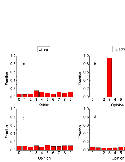
Figure 1: Final distribution of opinions for two different dynamics and two disorder parameters of $k$-SWN’s: a) Linear, $p_{d}=10^{-3}$, b) Quadratic, $p_{d}=10^{-3}$, c) Linear, $p_{d}=0.9$, d) Quadratic, $p_{d}=0.9$

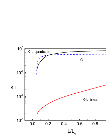
(a)

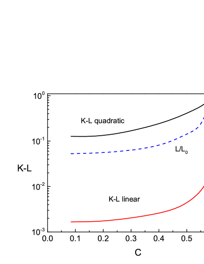
(b)

Figure 2: Normalized K-L distance, $D_{KL}/\log(N_{c})$, for different values of $p_{d}$ on $k$-SWNs and with linear and quadratic dynamics. a) as a function of $L/L_{o}$, with $L_{o}$ the mean path length of the ordered network. The dashed line is the value of $C$; b) as a function of $C$. The dashed line is the value of $L/L_{o}$.

IV Numerical results

Although different network topologies were used throughout our simulations, all of them consisted in $N=10000$ nodes and a mean degree $K_{m}=6$. The results were averaged over 500 realizations each. We will discuss each topology separately and contrast the obtained results whenever the comparison is relevant. We took $\rho=0.02$, that is within the range where a high interaction rate does not screen the dynamics. At higher values it can be observed a too fast convergence to consensus. On the other hand it is large enough to allow for enough interactions generate an effect in a reasonable time. The following results correspond to a navigation process that does not take into account the degree of the neighboring nodes at the moment of choosing the next steps. The differences with respect to another choice will be discussed later for SF networks.

IV.1 Final state of the dynamics

IV.1.1 $k$-SWN

As mentioned before, we took $N=10^{5}$, $K_{m}=K=2k=6$, and a disorder parameter $p_{d}$ ranging between 0 and 1. In order to characterize the formation of consensus we started by analyzing the change in the initially uniform distribution of messages. As expected, when the underlying dynamics is linear, there is a slight departure from the initial distribution due to unavoidable fluctuations. On the contrary, when nonlinear dynamics are considered the situation changes dramatically. This can be observed in Fig. 1, where we show the final distribution of opinions for the linear and quadratic dynamics, for two limiting cases, $p_{d}=10^{-3}$ and $p_{d}=.9$

The departure of the distribution of opinions from the initial one can be measured through the K-L distance. The difference between linear and quadratic dynamics are apparent throughout the whole range of $p_{d}$. In both cases, as the network disorder increases, the K-L distance decreases. In the linear case there is an increase but the distance is always at least one order of magnitude smaller than in the quadratic case. For the quadratic dynamics, it is possible to find an obvious reason in that as the mean path between nodes is smaller for disordered networks, a given agent takes less time to reach its target. This effect can be observed in Fig. 2a, where the values of the K-L distances are plotted against the average path length $L$. However, $L$ is not the only quantity that changes as a function of $p_{d}$. The clustering coefficient $C$ also decreases as the disorder grows and can be affecting the behavior of the K-L distance. The plot in Fig 2b shows the change in the K-L distance as a function of $C$. In both cases we observe two different regimes with slow and fast rates of change as a function of $L$ and $C$ respectively. We note that the fast change of the K-L distance in Fig. 2a corresponds to a range in which $C$ also changes rapidly as a function of $L$. The analogous situation is observed in Fig. 2b. We conclude that not only the change in path length contributes to the difference in the K-L distance but also the change in clustering. So far we have isolated the possible effect of a change in the degree distribution. In the next section this will be also taken into acount.

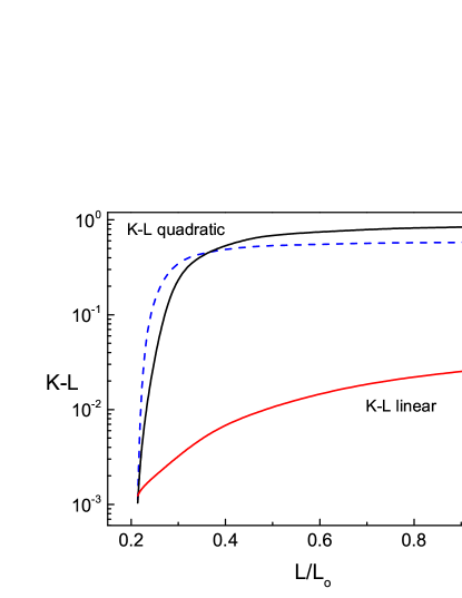
(a)

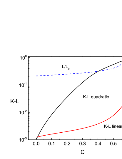
(b)

Figure 3: Normalized K-L distance for different values of $p_{d}$ on SWNs and with linear and quadratic dynamics. a) as a function of $L/L_{o}$, with $L_{o}$ the mean path length of the ordered network. The dashed line is the value of the clustering $C$; b) as a function of $C$. The dashed line is the value of $L/L_{o}$.

IV.1.2 SWN

While the construction of SW networks is similar to its regular version and also presents an analogous behavior in terms of the values of $C$ and $L$ as a function of the disorder coefficient, there exists an apparent difference. In addition to the effects of the topology on the formation of consensus due to the change of $C$ and $L$ we need to consider the effects that could arise due to the change in the degree distribution. As in the previous case, we observe a transition towards consensus that can be much better quantified by studying the behavior of the K-L distance. The plots in Figs. 3a and 3b show the dependence of the K-L distance on $C$ and $L$. In this case, we observe that the growth of the K-L distance behaves differently than the analogous situation in $k$-SWN for the quadratic dynamics, the one that promotes consensus formation. This difference must be due to the combined effect of an increase in $L$ and $C$ and a change in the degree distribution.

Indeed, if we compare both families of networks in a unique plot it is more evident that the spreading of the degree distribution goes against the formation of consensus. We show this in Fig 4, where we contrast the values of the K-L distance for the same values of clustering $C$ and mean path length $L$ for both types of networks. The figure shows that for the same values of clustering or path length, SWN networks start to fail in reaching consensus once the degree distribution has adopted a clear binomial profile, corresponding to lowest values of $C$ and $L$. A natural next step is to consider networks with more spanned degree distribution. A candidate for that are the Scale Free networks.

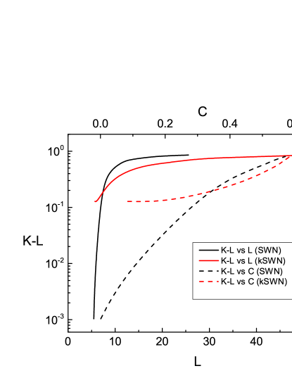
Figure 4: Comparison of the normalized K-L distance as a function of $L$ (lower $x$-axis,) and $C$ (upper $x$-axis).

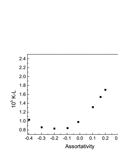
Figure 5: Normalized K-L distance for different values of assortativity $a$ on SF networks with quadratic dynamics.

Figure 6: Normalized K-L distance as a function of $p_{k}$ for a SF network with $a=0.4$, quadratic dynamics and degree dependent navigation strategy.

IV.1.3 SF Networks

So far we have studied SW networks with different degrees of disorder. The difference between SWN and $k$-SWN evidenced the effect of the heterogeneity of the degree distribution on the dynamics, that goes against the formation of consensus. SF networks owe their name to their particular degree distribution. We choose to analyze the behavior of the consensus emergence on these networks and compare it with our previous results. But SF networks are not only characterized by a degree distribution with a tail that falls with a power law. Among other properties, two networks might have the same degree distribution but present different assortativities. We choose to study the effect of this quantity in order to unveil the role of hubs or highly connected clusters of nodes in the obtained results. The calculated values of the K-L distance are low, as expected from previous results with highly disordered SW networks. The interesting feature of this case is associated to the behavior of the K-L distance as a function of the assortativity. We find that the emergence of a weak consensus corresponds to highly assortative or disassortative networks while neutral networks, that can also be linked to certain degree of heterogeneous structure, lead to its complete inhibition. This can be observed in Fig. 5. In any case we obtain much smaller values than in the small world network, in agreement with the result that long tails in the degree distribution impede the formation of consensus.

For this family of networks we have also studied a different navigation dynamics. Instead of choosing the next step at random, the choice pointed to the neighbor with the highest degree with probability $p_{k}$, and with complementary probability to any node in the neighborhood. The case $p_{k}=0$ corresponds to the previous one. While for neutral and disassortative SF networks we did not find any apparent difference, we noticed that this last strategy has an interest effect on assortative SF networks. As shown in Fig. 6, the consensus level increases with $p_{k}$, as the navigation strategy concentrates many of the walkers in a bounded subnet corresponding to those nodes with the highest degrees, allowing for the occurrence of much more interactions.

IV.2 Transient dynamics

Most of the features observed once the totality of agents have arrived to the target can be explained by analyzing the transient dynamics. We will discuss some of the most relevant observations in the following sections, starting with those aspects that only characterize the way the walkers navigate the network to finally address a characterization of the interactions rate, close linked to the consensus emergence.

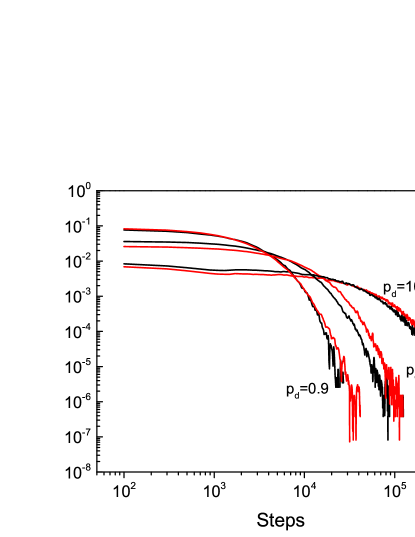
(a)

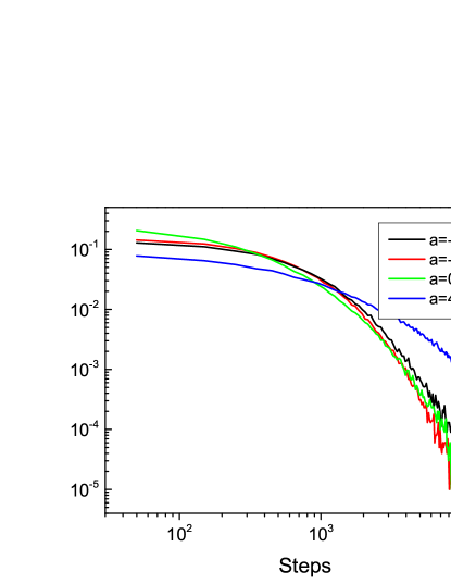
(b)

Figure 7: Step distribution for a) $k$-SWN (black) and SWN (red) , and b) SF networks

IV.2.1 Distribution of walking length

The process of consensus formation requires that the agents change their opinion in their way to their target destination. By studying the amount of steps a given agent needs to make from the origin to the destiny and knowing the probability of change of opinion at each step we can estimate the probability that an opinion has been altered. Though at first glance the results show us a trivial correlation between the length of the walks and the emergence of consensus or collapse of opinions, a closer analysis reveals same features that need to be observed with care. Fig. 7a shows the distribution of the number of steps (or walking length) for $k$-SWN and SWN for different disorder degrees. In Fig. 7b we plot the same for SF networks. As can be observed, there is a dramatic reduction in the number of required steps as the network gets more disordered. Despite the mentioned association between consensus emergence and longer walks, this plots shed no light about why the results for highly disordered $k$-SWN and SWN networks are so different, which have step distributions that are almost identical.

These last curves are very similar to those observed for SF networks. Besides, the plot corresponding to SF networks shows a non monotonic dependence on the assortativity. These results are consistent with what have been already shown in the previous section. Consensus formation is harder when the underlying network is only barely disassortative.

It is important to note that these results are independent of the choice of the dynamics and reveal only the topology of the walks. Though the distribution of walking length is directly linked to the performance of the networks in promoting consensus, it is not the only relevant feature, as has been already anticipated and will be further discussed in the following sections.

IV.2.2 Buffer dynamics

From the moment the agents start to reach their destination, the initial distribution of the number of agents in the nodes changes its shape, starting from a Gaussian-like distribution to turn into one with a high number of nodes with a low number of agents and a few with a high number of them. The rate of change of this distribution depends on the topology of the network. However, if we analyze these distributions as a function of the amount of arrived agents instead of the spent time we find, in the case of $k$-SWN that they are almost the same, as shown in Fig 8a where we plot the distribution of agents per node once 40% of the walkers have reached destination for several values pf $p_{d}$. Also shown in the same figure is the case for SWN. This time, the distributions do not overlap. We can observe that the curve corresponding to all the $k$-SWn and to the SWN with $p_{d}=10{-3}$ are overlapped. On the contrary, SWN with different disorder degrees present different behaviors. The last is also true for for SF networks with different assortativity values, as shown in Fig 8b.

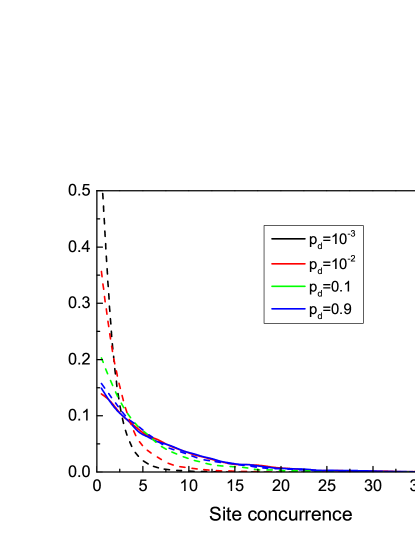
(a)

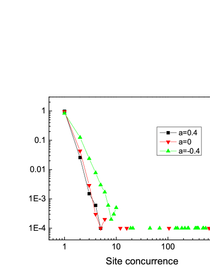
(b)

Figure 8: Distribution of the number of agents per node when 40% of packages has been delivered for a) $k$-SWN (solid) and SWN (dashed) , and b) SF networks

We start to sketch here a first explanation to the different behavior of the consensus on $k$-SWN and SWN. Together with a non linear interaction dynamics, the consensus requires the encounter and interaction of walkers to occur. The plots show us that the crowded sites are more abundant in $k$-SWN than in the others networks. This last fact promotes consensus formation.

IV.2.3 Opinion change dynamics

A natural question is at what stage of the dynamics occur the most part of the change of opinions. For that, we have recorded the rate of change occurrence and plotted it against the amount of agents that reached destination. While $k$-SWN and SWN show the same dynamics for low values of $p_{d}$, they are very different for higher disorder degrees. This is shown in Fig 9a. In highly disordered $K$-SWN the changes occur at the beginning of the dynamics (high number of mobile agents), while for SWN it is just the opposite. This is counterintuitive because the natural guess is to expect that most of the interactions occur when a high number of agents are still walking, as with $k$-SWN . In turn, SF networks behave as highly disordered SWN, but with a change rate much more concentrated at low values of walking agents, as shown in Fig 9b.

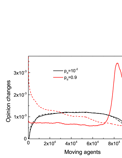
(a)

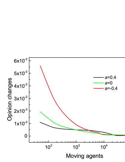
(b)

Figure 9: Changes of opinion as a function of the number of moving agents for a) $k$-SWN (solid) and SWN (dashed) , and b) SF networks

V Discussion

In the present work we have considered a model for the emergence of consensus in which the involved individuals are not influenced by static neighborhoods but participates from several dynamical fora where several individual gather and discuss. Different families of networks serve to mimic a variety of underlying topologies for these dynamical neighborhoods. The aim of of such election is to analyze how the particular properties of these topologies affect the emergence of consensus. By consensus we understand the collapse of different opinions into a single one. In turn, the opinions of the individuals is modeled as a scalar, ranging from 1 to 10 and without any notion of closeness between different opinions. That means that the opinion with value equal to 1 is not closer to the opinion with value equal to 2 than it is to another with value equal to 10. Our results suggest that an heterogeneous topology inhibits the formation of consensus. The heterogeneity in the considered networks is associated to a disordered structure, an extended degree distribution and the lack of correlation between nodes degree.

We have shown that a linear interaction dynamics, that consist only in a replacement of and idea by other one does not promote consensus. On the contrary, what we called quadratic dynamics favors the propagation of coincidences, leading to consensus. We have also considered some alternative dynamical rules with results that are analogous to what we have obtained for the quadratic one. Though they were not discussed in this work they are worth mentioning. These dynamics are

• Higher order $n$: Analogous to the quadratic taking $n$ opinions among the present in the node.

• Poissonian: The number $n$ considered in the previous case is taken from a Poisson distribution.

• Uniform: As in the previous case, with a $n$ uniformly distributed.

As mentioned before, the results are qualitatively the same to which we obtained with the quadratic dynamics, suggesting that the quadratic case represents a generic non-linear interaction. However it must me notice that for a purely case that finite size effects become more severe than for the quadratic, because the change of opinion now requires that there are at least three agents in node.

The present results can be also interpreted in a different framework such as errors in the transmission of information. When considering information transfer, the occurrence of errors during the process is of fundamental interest. Therefore, any realistic process of transfer information should include the possibilities of making mistakes that can degrade the performance of the system. These mistakes can be assumed to take the form of random processes that occur in parallel to the transmission of information. It is usually assumed that the mistakes affect the directions to which the packets of information are being delivered. For instance, a package could be delivered to a random networks node instead of its desired destination or the topology of the network could be perturbed for all the messages that go through a given region. These aspects have been analyzed in ref. czaplicka . Interestingly, it is found that in some cases this kind of noise can enhance transfer of information via a phenomenon similar to stochastic resonance, with a non trivial interaction between the two types of noise. But we can have also the possibility that noise does not affect the destination of the messages but its content. This is the equivalent of what here, with the opinions of the agents take the place of the content of the messages.

References

- (1) S. Boccaletti , V. Latora, Y. Moreno, M. Chavez, D.-U. Hwang, Phys. Rep. 424, 175–308 (2006)
- (2) M. Kuperman, G. Abramson, Phys. Rev. Lett. 86, 2909. (2001)
- (3) G. Abramson and M. Kuperman Phys. Rev. E 63, 030901R (2001)
- (4) M.N. Kuperman Phys. Rev. E 73, 046139 (2006)
- (5) M.O. Jackson, B. Rogers, Advan. Theoret. Econ. 7, 1–13 (2007)
- (6) D. López-Pintado, Games and Economic Behavior 62, 573–590 (2008)
- (7) J. Gómez-Gardeñes, V. Latora Phys. Rev. E 78, 065102(R) (2008)
- (8) H. Wang, Shang, L. Physica A 421, 180-186 (2015)
- (9) M. H. DeGroot, Journal of the American Statistical Association 69, 118-121 (1974)
- (10) R. L. Berger, Journal of the American Statistical Association 76, 415-418 (1981)
- (11) G. L. Gilardoni, M. K. Clayton, The Annals of Statistics, 391-401 (1993)
- (12) R. A. Holley, T. M. Liggett, The annals of probability, 643-663 (1975)
- (13) K. Sznajd-Weron, J. Sznajd, International Journal of Modern Physics C 11, 1157-1165 (2000)
- (14) P. M. DeMarzo, D. Vayanos, J. Zwiebel, The Quarterly Journal of Economics 118, 909-968 (2003)
- (15) A. Fazeli, A. Jadbabaie, In Decision and Control and European Control Conference (CDC-ECC), 2011 50th IEEE Conference on (pp. 2341-2346). (IEEE, 2011).
- (16) M. Barthélemy, A. Barrat, R. Pastor-Satorras, A. Vespignani Phys. Rev. Lett. 92, 178701 (2004).
- (17) L. Huang, K. Park, Y. C. Lai, Phys. Rev. E 73, 035103-R (2006)
- (18) D.J. Watts, S.H. Strogatz, Nature 393, 440 (1998)
- (19) M. N. Kuperman, S. Risau-Gusman, Eur. Phys. J. B 62, 233–238 (2008)
- (20) A. Barrat, M Weigt, Eur. Phys. J. B. 13, 547–560 (2000)
- (21) A. L. Barabási, R. Albert, Science 286, 509 (1999)
- (22) R. Xulvi-Brunet, I. M. Sokolov, Phys. Rev. E 70, 066102 (2004)
- (23) M.E.J. Newman. Phys. Rev. Lett. 89, 208701 (2002)
- (24) B.J. Kim, C.N. Yoon, S.K. Han, H. Jeong, Phys. Rev. E 65, 27103 (2002)
- (25) J.D. Noh, H. Rieger, Phys. Rev. Lett. 92, 118701 (2004)
- (26) L. Adamic, R.M. Lukose, A.R. Puniyani, B.A. Huberman, Phys. Rev. E 64, 46135 (2001)
- (27) S. Kullback, R. A. Leibler, Annals of Mathematical Statistics 22, 79–86 (1951)
- (28) A. Czaplicka, J. A. Holyst , P. M. A. Sloot, Scientific Reports 3 1223 (2013)