New stabilized discretizations for poroelasticity and the Stokes’ equations

Abstract

In this work, we consider the popular P1-RT0-P0 discretization of the three-field formulation of Biot’s consolidation problem. Since this finite-element formulation does not satisfy an inf-sup condition uniformly with respect to the physical parameters, several issues arise in numerical simulations. For example, when the permeability is small with respect to the mesh size, volumetric locking may occur. Thus, we propose a stabilization technique that enriches the piecewise linear finite-element space of the displacement with the span of edge/face bubble functions. We show that for Biot’s model this does give rise to discretizations that are uniformly stable with respect to the physical parameters. We also propose a perturbation of the bilinear form, which allows for local elimination of the bubble functions and provides a uniformly stable scheme with the same number of degrees of freedom as the classical P1-RT0-P0 approach. We prove optimal stability and error estimates for this discretization. Finally, we show that this scheme can also be successfully applied to Stokes’ equations, yielding a discrete problem with optimal approximation properties and with minimum number of degrees of freedom (equivalent to a P1-P0 discretization). Numerical tests confirm the theory for both poroelastic and Stokes’ test problems.

1 Introduction

The interaction between the deformation and fluid flow in a fluid-saturated porous medium is the object of study in poroelasticity theory. Such coupling has been modelled in the early one-dimensional work of Terzaghi [1]. A more general three-dimensional mathematical formulation was then established by Maurice Biot in several pioneering publications (see [2] and [3]). Biot’s models are widely used nowadays in the modeling of many applications in different fields, ranging from geomechanics and petroleum engineering, to biomechanics. The existence and uniqueness of the solution for these problems have been investigated by Showalter in [4] and by Zenisek in [5]. Regarding the numerical simulation of the poroelasticity equations, there have been numerous contributions using finite-difference schemes [6, 7] and finite-volume methods (see [8] for recent developments). Finite-element methods, which are the subject of this work, have also been considered (see for example the monograph by Lewis and Schrefler [9] and the references therein).

Stable finite-element schemes are constructed by either choosing discrete spaces satisfying appropriate inf-sup (or LBB) conditions, or applying suitable stabilization techniques to unstable finite-element pairs. For the two-field (displacements-pressure) formulation of Biot’s problem, the classical Taylor-Hood elements belong to the first class [10, 11, 12], as well as the MINI element [13]. On the other hand, a stabilized discretization based on linear finite elements for both displacements and pressure has been recently analyzed in [13], and belongs to the second type. Regarding three-field formulations (including the Darcy velocity), a stable finite-element method based on non-conforming Crouzeix-Raviart finite elements for the displacements, lowest order Raviart-Thomas-Nédélec elements for the Darcy velocity, and piecewise constants for the pressure, was proposed in [14]. For a four-field formulation of the problem, which includes the stress tensor, the fluid flux, the solid displacement, and the pore pressure as unknowns, a stable approach is proposed in [15]. In that work, two mixed finite elements, one for linear elasticity and one for mixed Poisson, are coupled for the spatial discretization.

This paper focuses on the three-field formulation, which has received a lot of attention from the point of view of novel discretizations [16, 17, 18, 19], as well as for the design of efficient solvers [20, 21, 22]. Because of its application to existing reservoir engineering simulators, one of the most frequently considered schemes is a three-field formulation based on piecewise linear elements for displacements, Raviart-Thomas-Nédélec elements for the fluid flux, and piecewise constants for the pressure. This element, however, does not satisfy an inf-sup condition uniformly with respect to the physical parameters of the problem. Thus, we propose a stabilization of this popular element which gives rise to uniform error bounds, keeping the same number of degrees of freedom as in the original method.

A consequence of our analysis is that a new stable scheme for the Stokes’ equations is derived. The resulting method can be seen as a perturbation of the well-known unstable pair based on piecewise linear and piecewise constant elements for velocities and pressure, respectively (P1-P0). This yields a stable finite-element pair for Stokes, which has the lowest possible number of degrees of freedom.

The rest of the paper is organized as follows. Section 2 is devoted to describing Biot’s problem and, in particular, the considered three-field formulation and its discretization. A numerical example is given, illustrating the difficulties that appear. In Section 3, we introduce the stabilized scheme in which we consider the enrichment of the piecewise linear continuous finite-element space with edge/face (2D/3D) bubble functions. Section 4 is devoted to the local elimination of the bubbles to maintain the same number of degrees of freedom as in the original scheme. The well-posedness of the resulting scheme, as well as the corresponding error analysis are also provided here. In Section 5, we present the Stokes-stable finite-element method based on P1-P0 finite elements obtained by following the same strategy as presented in the previous sections for poroelasticity. Finally, in Section 6, we confirm the uniform convergence properties of the stabilized schemes for both poroelasticity and Stokes’ equations through some numerical tests.

2 Preliminaries: model problem and notation

We consider the quasi-static Biot’s model for consolidation in a linearly elastic, homogeneous, and isotropic porous medium saturated by an incompressible Newtonian fluid. According to Biot’s theory [2], the mathematical model of the consolidation process is described by the following system of partial differential equations (PDEs) in a domain $\Omega\subset\mathbb{R}^{d}$, $d=2,3$ with sufficiently smooth boundary $\Gamma=\partial\Omega$:

equilibrium equation: $$-{\rm div}\,{\bm{\sigma}}^{\prime}+\alpha\nabla\,p=\rho{\bm{g}},\quad{\rm in}\,\Omega,$$ (1)

constitutive equation: $$\bm{\sigma}^{\prime}=2\mu{\bm{\varepsilon}}(\bm{u})+\lambda\operatorname{div}(\bm{u}){\bm{I}},\quad{\rm in}\,\Omega,$$ (2)

compatibility condition: $${\bm{\varepsilon}}({\bm{u}})=\frac{1}{2}(\nabla{\bm{u}}+\nabla{\bm{u}}^{t}),\quad{\rm in}\,\Omega,$$ (3)

Darcy’s law: $${\bm{w}}=-\displaystyle\frac{1}{\mu_{f}}{\bm{K}}(\nabla p-\rho_{f}{\bm{g}}),\quad{\rm in}\,\Omega,$$ (4)

continuity equation: $$\displaystyle\frac{\partial}{\partial t}\left(\frac{1}{M}p+\alpha\ {\operatorname{div}}\,{\bm{u}}\right)+{\operatorname{div}}\,{\bm{w}}=f,\quad{\rm in}\,\Omega,$$ (5)

where $\lambda$ and $\mu$ are the Lamé coefficients, $M$ is the Biot modulus, and $\displaystyle\alpha=1-\frac{K_{b}}{K_{s}}$ is the Biot-Willis constant. Here, $K_{b}$ and $K_{s}$ denote the drained and the solid phase bulk moduli. As is customary, ${\bm{K}}$ stands for the absolute permeability tensor, $\mu_{f}$ is the viscosity of the fluid, and $\bm{I}$ is the identity tensor. The unknown functions are the displacement vector ${\bm{u}}$ and the pore pressure $p$. The effective stress tensor and the strain tensor are denoted by ${\bm{\sigma}}^{\prime}$ and $\bm{\varepsilon}$, respectively. The percolation velocity of the fluid, or Darcy’s velocity, relative to the soil is denoted by $\bm{w}$ and the vector-valued function ${\bm{g}}$ represents the gravitational force. The bulk density is $\rho=\phi\rho_{f}+(1-\phi)\rho_{s}$, where $\rho_{s}$ and $\rho_{f}$ are the densities of solid and fluid phases and $\phi$ is the porosity. Finally, the source term $f$ represents a forced fluid extraction or injection process.

Our focus here is on the so-called three-field formulation in which Darcy’s velocity, ${\bm{w}}$, is also a primary unknown in addition to ${\bm{u}}$ and $p$. As a result, we have the following system of PDEs:

$$-\operatorname{div}\bm{\sigma}^{\prime}+\alpha\nabla p=\rho\bm{g},\qquad\mbox{where}\quad\bm{\sigma}^{\prime}=2\mu{\bm{\varepsilon}}(\bm{u})+\lambda\operatorname{div}(\bm{u})\bm{I},$$ (6)

$${\bf K}^{-1}\mu_{f}{\bm{w}}+\nabla p=\rho_{f}{\bm{g}},$$ (7)

$$\displaystyle\frac{\partial}{\partial t}\left(\frac{1}{M}p+\alpha\ {\operatorname{div}}\,{\bm{u}}\right)+{\operatorname{div}}\,{\bm{w}}=f.$$ (8)

This system is often subject to the following set of boundary conditions:

$$p=0,\quad\mbox{for}\quad x\in\overline{\Gamma}_{t},\quad\bm{\sigma}^{\prime}\,{\bm{n}}={\bm{0}},\quad\quad\mbox{for}\quad x\in\Gamma_{t},$$ (9)

$${\bm{u}}={\bm{0}},\quad\mbox{for}\quad x\in\overline{\Gamma}_{c},\quad{\bm{w}}\cdot{\bm{n}}=0,\quad\mbox{for}\quad x\in\Gamma_{c},$$ (10)

where ${\bm{n}}$ is the outward unit normal to the boundary, $\overline{\Gamma}=\overline{\Gamma}_{t}\cup\overline{\Gamma}_{c}$, with $\Gamma_{t}$ and $\Gamma_{c}$ being open (with respect to $\Gamma$) subsets of $\Gamma$ with nonzero measure. In the following, we omit the symbol “$\overline{~{}~{}}$” over $\Gamma_{t}$ and $\Gamma_{c}$ as it will be clear from the context that the essential boundary conditions are imposed on closed subsets of $\Gamma$. Other sets of boundary conditions are also of interest, such as full Dirichlet conditions for both $p$ and $\bm{u}$ on all of $\Gamma$.

The initial condition at $t=0$ is given by,

$$\left(\frac{1}{M}p+\alpha\operatorname{div}{\bm{u}}\right)\,(\bm{x},0)=0,\,\bm{x}\in\Omega,$$ (11)

which yields the following mixed formulation of Biot’s three-field consolidation model:
For each $t\in(0,T]$, find $(\bm{u}(t),\bm{w}(t),p(t))\in\bm{V}\times\bm{W}\times Q$ such that

$$a(\bm{u},\bm{v})-(\alpha p,\operatorname{div}\bm{v})=(\rho\bm{g},\bm{v}),\quad\forall\ \bm{v}\in\bm{V},$$ (12)

$$({\bm{K}}^{-1}\mu_{f}\bm{w},\bm{r})-(p,\operatorname{div}\bm{r})=(\rho_{f}{\bm{g}},\bm{r}),\quad\forall\ \bm{r}\in\bm{W},$$ (13)

$$\left(\frac{1}{M}\frac{\partial p}{\partial t},q\right)+\left(\alpha\operatorname{div}\frac{\partial\bm{u}}{\partial t},q\right)+(\operatorname{div}\bm{w},q)=(f,q),\quad\forall\ q\in Q,$$ (14)

where,

$$a(\bm{u},\bm{v})=2\mu\int_{\Omega}{\bm{\varepsilon}}(\bm{u}):{\bm{\varepsilon}}(\bm{v})+\lambda\int_{\Omega}\operatorname{div}\bm{u}\operatorname{div}\bm{v},$$ (15)

corresponds to linear elasticity. The function spaces used in the variational form are

$${\bm{V}}=\{{\bm{u}}\in{\bm{H}}^{1}(\Omega)\ |\ {\bm{u}}|_{\overline{\Gamma}_{c}}={\bm{0}}\},$$

$${\bm{W}}=\{{\bm{w}}\in\bm{H}(\operatorname{div},\Omega)\ |\ ({\bm{w}}\cdot{\bm{n}})|_{\Gamma_{c}}=0\},$$

$$Q=L^{2}(\Omega),$$

where ${\bm{H}}^{1}(\Omega)$ is the space of square integrable vector-valued functions whose first derivatives are also square integrable, and $\bm{H}(\operatorname{div},\Omega)$ contains the square integrable vector-valued functions with square integrable divergence.

We recall that the well-posedness of the continuous problem was established by Showalter [4], and, for the three-field formulation by Lipnikov [23]. Next, we focus on the behavior of some classical discretizations of Biot’s model.

2.1 Discretizations

First, we partition the domain $\Omega$ into $n$-dimensional simplices and denote the resulting partition with $\mathcal{T}_{h}$, i.e., $\overline{\Omega}=\cup_{T\in\mathcal{T}_{h}}\overline{T}$. Further, with every simplex $T\in\mathcal{T}_{h}$, we associate two quantities which characterize its shape: the diameter of $T$, $h_{T}=\operatorname{diam}(T)$, and the radius, $\rho_{T}$, of the $n$-dimensional ball inscribed in $T$. The simplicial mesh is shape regular if and only if $h_{T}/\rho_{T}\lesssim 1$ uniformly with respect to $T$.

With the partitioning, $\mathcal{T}_{h}$, we associate a triple of piecewise polynomial, finite-dimensional spaces,

$$\bm{V}_{h}\subset\bm{V},\quad\bm{W}_{h}\subset\bm{W},\quad Q_{h}\subset Q.$$ (16)

While we specify two choices of the space $\bm{V}_{h}$ later, we fix $\bm{W}_{h}$ and $Q_{h}$ as follows,

$${\bm{W}}_{h}=\{{\bm{w}}_{h}\in\bm{W}\ |\ {\bm{w}}_{h}|_{T}={\bm{a}}+\eta{\mathbf{x}},\ {\bm{a}}\in{\mathbb{R}}^{d},~{}\eta\in{\mathbb{R}},\ \ \forall\,T\in\mathcal{T}_{h}\},$$

$$Q_{h}=\{q_{h}\in Q\ |\ q_{h}|_{T}\in{\mathbb{P}}_{0}(T),\ \ \forall\,T\in\mathcal{T}_{h}\},$$

where ${\mathbb{P}}_{0}(T)$ is the one-dimensional space of constant functions on $T$. We note that the inclusions listed in (16) imply that the elements of $\bm{V}_{h}$ are continuous on $\Omega$, the functions in $\bm{W}_{h}$ have continuous normal components across element boundaries, and that the functions in $Q_{h}$ are in $L^{2}(\Omega)$. This choice of $\bm{W}_{h}$ is the standard lowest order Raviart-Thomas-Nédélec space (RT0) and $Q_{h}$ is the piecewise constant space (P0).

Finally, using backward Euler as a time discretization on a time interval $(0,t_{\max{}}]$ with constant time-step size $\tau$, the discrete scheme corresponding to the three-field formulation (12)-(14) reads:
Find $(\bm{u}_{h}^{m},\bm{w}_{h}^{m},p_{h}^{m})\in\bm{V}_{h}\times\bm{W}_{h}\times Q_{h}$ such that

$$a(\bm{u}_{h}^{m},\bm{v}_{h})-(\alpha p_{h}^{m},\operatorname{div}\bm{v}_{h})=(\rho\bm{g},\bm{v}_{h}),\quad\forall\ \bm{v}_{h}\in\bm{V}_{h},$$ (17)

$$\tau({\bm{K}}^{-1}\mu_{f}\bm{w}_{h}^{m},\bm{r}_{h})-\tau(p_{h}^{m},\operatorname{div}\bm{r}_{h})=\tau(\rho_{f}{\bm{g}},\bm{r}_{h}),\quad\forall\ \bm{r}_{h}\in\bm{W}_{h},$$ (18)

$$\left(\frac{1}{M}p^{m}_{h},q_{h}\right)+\left(\alpha\operatorname{div}\bm{u}_{h}^{m},q_{h}\right)+\tau(\operatorname{div}\bm{w}_{h}^{m},q_{h})=(\widetilde{f},q_{h}),\quad\forall\ q_{h}\in Q_{h},$$ (19)

where $(\widetilde{f},q_{h})=\tau(f,q_{h})+\left(\frac{1}{M}p^{m-1}_{h},q_{h}\right)+\left(\alpha\operatorname{div}\bm{u}_{h}^{m-1},q_{h}\right)$, and,

$$(\bm{u}_{h}^{m},\bm{w}_{h}^{m},p_{h}^{m})\approx\left(\bm{u}(\cdot,t_{m}),\bm{w}(\cdot,t_{m}),p(\cdot,t_{m})\right),\quad t_{m}=m\tau,\ m=1,2,\ldots$$

2.2 Effects of permeability on the error of approximation

For $\bm{V}_{h}$, we start with a popular finite-element approximation for (12)–(14) by choosing

$$\bm{V}_{h}=\bm{V}_{h,1},\quad\mbox{with}\quad\bm{V}_{h,1} := \{{\bm{v}}_{h}\in{\bm{V}}\;\big{|}\;{\bm{v}}_{h}|_{T}\in[{\mathbb{P}}_{1}(T)]^{d},~{}\mbox{for all}~{}T\in\mathcal{T}_{h}\},$$

where $\mathbb{P}_{1}(T)$ is the space of linear polynomials on $T\in\mathcal{T}_{h}$. Then, $\bm{V}_{h,1}$ is the space of piecewise linear (with respect to $\mathcal{T}_{h}$), continuous vector-valued functions. For uniformly positive definite permeability tensor, $\bm{K}$, such choice of spaces has been successfully employed for numerical simulations of Biot’s consolidation model (see [18, 23]). However, the heuristic considerations that expose some of the issues with this discretization are observed in cases when $\bm{K}\to\bm{0}$. In such cases, $\bm{w}\to\bm{0}$ and the discrete problem approaches a P1-P0 discretization of the Stokes’ equation. As it is well known, the element pair, $\bm{V}_{h,1}\times Q_{h}$, does not satisfy the inf-sup condition and is unstable for the Stokes’ problem. In fact, on a uniform grid in $2D$, it is easy to prove that volumetric locking occurs, namely, that the only divergence-free function from $\bm{V}_{h,1}$ is the zero function. More precisely,

$$\operatorname{dim}(Q_{h})>\operatorname{dim}\bm{V}_{h}>\operatorname{dim}\operatorname{Range}(\operatorname{div}_{h}),\quad\operatorname{div}_{h}=\operatorname{div}\big{|}_{\bm{V}_{h}}.$$

These inequalities imply that $\operatorname{div}_{h}$ is not an onto operator, and, hence, the pair of spaces violates the inf-sup condition  [24] associated with the discrete Stokes’ problem. More details on this undesirable phenomenon for Stokes are found in the classical monograph [24] and also in [25, pp. 45–100] and [26].

Here, we demonstrate numerically that for Biot’s model, the error in the finite-element approximation does not decrease when the permeability is small relative to the mesh size. We consider $\Omega=(0,1)\times(0,1)$, and approximate (12)-(14) subject to Dirichlet boundary conditions for both $\bm{u}$ and $p$ on the whole of $\Gamma$. We cover $\Omega$ with a uniform triangular grid by dividing an $(N\times N)$ uniform square mesh into right triangles. The material parameters are $\lambda=2$, $\mu=1$, $\mu_{f}=1$, $\alpha=1$, and $M=10^{6}$. We consider a diagonal permeability tensor ${\bm{K}}=k{\bm{I}}$ with constant $k$, and the other data is set so that the exact solution is given by

$$\bm{u}(x,y,t) = \operatorname{curl}\varphi=\begin{pmatrix}\partial_{y}\varphi\\ -\partial_{x}\varphi\end{pmatrix},\quad\varphi(x,y)=[xy(1-x)(1-y)]^{2},$$

$$p(x,y,t) = 1.$$

Finally, we set $\tau=1$ and $t_{\max{}}=1$, so that we only perform one time step.

As seen in Table 2.1 the energy norm ($\|\bm{v}\|_{A}^{2}:=a(\bm{v},\bm{v})$ for $\bm{v}\in\bm{V}$) for the displacement errors and the $L^{2}$-norm for pressure errors do not decrease until the mesh size is sufficiently small (compared with the permeability). Thus for small permeabilities, this could result in expensive discretizations which are less applicable to practical situations.

	$8$	$16$	$32$	$64$	$128$
$10^{-4}$	$0.0187$	$0.0040$	$0.0009$	$0.0002$	$5.66\times 10^{-5}$	$\|\Pi_{1}{\bm{u}}-{\bm{u}}_{h}\|_{A}$
	$0.0590$	$0.0090$	$0.0016$	$0.0003$	$8.33\times 10^{-5}$	$\|\Pi_{0}p-p_{h}\|_{L^{2}}$
$10^{-6}$	$0.0547$	$0.0302$	$0.0050$	$0.0005$	$8.93\times 10^{-5}$	$\|\Pi_{1}{\bm{u}}-{\bm{u}}_{h}\|_{A}$
	$0.3187$	$0.3098$	$0.0741$	$0.0097$	$0.0012$	$\|\Pi_{0}p-p_{h}\|_{L^{2}}$
$10^{-8}$	$0.0578$	$0.0567$	$0.0476$	$0.0165$	$0.0018$	$\|\Pi_{1}{\bm{u}}-{\bm{u}}_{h}\|_{A}$
	$0.3388$	$0.7067$	$1.1418$	$0.6450$	$0.1142$	$\|\Pi_{0}p-p_{h}\|_{L^{2}}$
$10^{-10}$	$0.0578$	$0.0574$	$0.0570$	$0.0550$	$0.0502$	$\|\Pi_{1}{\bm{u}}-{\bm{u}}_{h}\|_{A}$
	$0.3372$	$0.7176$	$1.4527$	$2.7790$	$3.4403$	$\|\Pi_{0}p-p_{h}\|_{L^{2}}$

Table 2.1: Energy norm and $L^{2}$-norm for displacement and pressure errors, respectively. Hydraulic conductivity: $\kappa=(k/\mu_{f})=10^{-2\nu}$, $\nu=2,\ldots,5$; grid parameters: $h=2^{-l}$ and $N=2^{l}$, $l=3,\ldots,7$. Results confirm poor approximation when $\kappa/h$ is small, where $\kappa=k/\mu_{f}$.

3 Stabilization and perturbation of the bilinear form

To resolve the above issue, we introduce a well-known stabilization technique based on enrichment of the piecewise linear continuous finite-element space, $\bm{V}_{h,1}$, with edge/face (2D/3D) bubble functions (see [27, pp. 145-149]). The discretization described below is based on a Stokes-stable pair of spaces $(\bm{V}_{h},Q_{h})$ with $\bm{V}_{h}\supset\bm{V}_{h,1}$. As we show later, in Section 4, this stabilization gives a proper finite-element approximation of the solution of Biot’s model independently of the size of the hydraulic conductivity, $\kappa$.

3.1 Stabilization by face bubbles

To define the enriched space, following [27], consider the set of $(d-1)$ dimensional faces from $\mathcal{T}_{h}$ and denote this set by $\mathcal{E}=\mathcal{E}^{o}\cup\mathcal{E}^{\partial}$, where $\mathcal{E}^{o}$ is the set of interior faces (shared by two elements) and $\mathcal{E}^{\partial}$ is the set of faces on the boundary. In addition, $\mathcal{E}^{\Gamma_{t}}$ is the set of faces on the boundary $\Gamma_{t}$ and $\mathcal{E}^{o,t}=\mathcal{E}^{o}\cap\mathcal{E}^{\Gamma_{t}}$. Note, if $\Gamma_{t}=\partial\Omega$ (pure traction boundary condition), then $\mathcal{E}^{\Gamma_{t}}=\mathcal{E}^{\partial}$ and $\mathcal{E}^{o,t}=\mathcal{E}$. For any face $e\in\mathcal{E}^{o}$, such that $e\in\partial T$, and $T\in\mathcal{T}_{h}$, let $\bm{n}_{e,T}$ be the outward (with respect to $T$) unit normal vector to $e$. With every face $e\in\mathcal{E}^{o}$, we also associate a unit vector $\bm{n}_{e}$ which is orthogonal to it. Clearly, if $e\in\partial T$ we have $\bm{n}_{e}=\pm\bm{n}_{e,T}$. For the boundary faces $e\in\mathcal{E}^{\partial}$, we always set $\bm{n}_{e}=\bm{n}_{e,T}$, where $T$ is the unique element for which we have $e\subset\partial T$. For the interior faces, the particular direction of $\bm{n}_{e}$ is not important, although it is important that this direction is fixed. More precisely,

$$\bm{n}_{e}=\bm{n}_{e,T^{+}}=-\bm{n}_{e,T^{-}}\quad\mbox{if}\quad e=T^{+}\cap T^{-},\quad\mbox{and}\quad T^{\pm}\in\mathcal{T}_{h},$$ (20)

Further, with every face $e\in\mathcal{E}$, $e=T^{+}\cap T^{-}$, we associate a vector-valued function $\bm{\Phi}_{e}$,

$$\bm{\Phi}_{e}=\varphi_{e}\bm{n}_{e},\quad\mbox{with}\quad\varphi_{e}\bigg{|}_{T^{\pm}}=\varphi_{e,T^{\pm}},\quad\mbox{and}\quad\varphi_{e,T^{\pm}}=\prod_{k=1,k\neq j^{\pm}}^{d+1}\lambda_{k,T^{\pm}},$$ (21)

where $\lambda_{k,T^{\pm}}$, $k=1,\ldots,(d+1)$ are barycentric coordinates on $T^{\pm}$ and $j^{\pm}$ is the vertex opposite to the face $e$ in $T^{\pm}$. We note that $\bm{\Phi}_{e}\in{\bm{V}}$ is a continuous piecewise polynomial function of degree $d$.

Finally, the stabilized finite-element space $\bm{V}_{h}$ is defined as

$${\bm{V}}_{h}=\bm{V}_{h,1}\oplus\bm{V}_{b},\quad\bm{V}_{b}=\operatorname{span}\{\bm{\Phi}_{e}\}_{e\in\mathcal{E}^{o,t}}.$$ (22)

The degrees of freedom associated with $\bm{V}_{h}$ are the values at the vertices of $\mathcal{T}_{h}$ and the total flux through $e\in\mathcal{E}^{o,t}$ of $(I-\Pi_{1}){\bm{v}}_{h}$, where $\Pi_{1}$ is the standard piecewise linear interpolant, $\Pi_{1}:C(\overline{\Omega})\mapsto\bm{V}_{h,1}$. Then, the canonical interpolant, $\Pi:C(\overline{\Omega})\mapsto\bm{V}_{h}$, is defined as:

$$\Pi\bm{v}=\Pi_{1}\bm{v}+\sum_{e\in\mathcal{E}^{o,t}}v_{e}\bm{\Phi}_{e},\quad v_{e}=\frac{1}{|e|}\int_{e}(I-\Pi_{1})\bm{v}.$$

With this choice of $\bm{V}_{h}$, the variational form, (17)–(19), remains the same and we have the following block form of the discrete problem:

$$\mathcal{A}\left(\begin{array}[]{c}{\bm{U}}_{b}\\ {\bm{U}}_{l}\\ {\bm{W}}\\ {\bm{P}}\end{array}\right)={\bm{b}},\ \ \hbox{with}\ \ \mathcal{A}=\left(\begin{array}[]{cccc}A_{bb}&A_{bl}&0&G_{b}\\ A_{bl}^{T}&A_{ll}&0&G_{l}\\ 0&0&\tau M_{w}&\tau G\\ G_{b}^{T}&G_{l}^{T}&\tau G^{T}&-M_{p}\end{array}\right),$$ (23)

where ${\bm{U}}_{b}$, ${\bm{U}}_{l}$, ${\bm{W}}$ and ${\bm{P}}$ are the unknown vectors for the bubble components of the displacement, the piecewise linear components of the displacement, the Darcy velocity, and the pressure, respectively. The blocks in the definition of $\mathcal{A}$ correspond to the following bilinear forms:

$$a(\bm{u}_{h}^{b},\bm{v}_{h}^{b})\rightarrow A_{bb},\quad a(\bm{u}_{h}^{l},\bm{v}_{h}^{b})\rightarrow A_{bl},\quad a(\bm{u}_{h}^{l},\bm{v}_{h}^{l})\rightarrow A_{ll},$$

$$-(\alpha p_{h},\operatorname{div}\bm{v}_{h}^{b})\rightarrow G_{b},\quad-(\alpha p_{h},\operatorname{div}\bm{v}_{h}^{l})\rightarrow G_{l},\quad-(p_{h},\operatorname{div}\bm{r}_{h})\rightarrow G,$$

$$(K^{-1}\mu_{f}\bm{w}_{h},\bm{r}_{h})\rightarrow M_{w},\quad\left(\frac{1}{M}p_{h},q_{h}\right)\rightarrow M_{p},$$

where ${\bm{u}}_{h}={\bm{u}}_{h}^{l}+{\bm{u}}_{h}^{b}$, ${\bm{u}}_{h}^{l}\in\bm{V}_{h,1}$, ${\bm{u}}_{h}^{b}\in\bm{V}_{b}$, and an analogous decomposition for $\bm{v}_{h}$.

Next, we define the following notion of stability for discretizations of Biot’s model needed for the analysis.

Definition 3.1.

The triple of spaces $(\widetilde{\bm{V}}_{h},\widetilde{\bm{W}}_{h},\widetilde{Q}_{h})$ is Stokes-Biot stable if and only if the following conditions are satisfied:

• $a(\bm{u}_{h},\bm{v}_{h})\leq C_{\bm{V}}\|\bm{u}_{h}\|_{1}\|\bm{v}_{h}\|_{1}$, for all $\bm{u}_{h}\in\widetilde{\bm{V}}_{h}$, $\bm{v}_{h}\in\widetilde{\bm{V}}_{h}$;

• $a(\bm{u}_{h},\bm{u}_{h})\geq\alpha_{\bm{V}}\|\bm{u}_{h}\|_{1}^{2}$, for all $\bm{u}_{h}\in\widetilde{\bm{V}}_{h}$;

• The pair of spaces $(\widetilde{\bm{W}}_{h},\widetilde{Q}_{h})$ is Poisson stable, i.e., it satisfies stability and continuity conditions required by the mixed discretization of the Poisson equation;

• The pair of spaces $(\widetilde{\bm{V}}_{h},\widetilde{Q}_{h})$ is Stokes stable.

Here, $\|\cdot\|_{1}$ and $\|\cdot\|$ denote the standard ${\bm{H}}^{1}$ norm and $L^{2}$ norm, respectively.

To show how stability for the Biot’s system follows from the conditions above, we introduce a norm on $\bm{V}_{h}\times{\bm{W}}_{h}\times Q_{h}$:

$$\|({\bm{u}}_{h},{\bm{w}}_{h},p_{h})\|_{\tau}=\left(\|{\bm{u}}_{h}\|_{1}^{2}+\tau\|{\bm{w}}_{h}\|^{2}+\tau^{2}\|\operatorname{div}{\bm{w}}_{h}\|^{2}+\|p_{h}\|^{2}\right)^{1/2},$$ (24)

Further, we associate a composite bilinear form on the space, $\bm{V}_{h}\times{\bm{W}}_{h}\times Q_{h}$,

$$B(\bm{u}_{h},\bm{w}_{h},p_{h};\bm{v}_{h},\bm{r}_{h},q_{h}) := a(\bm{u}_{h},\bm{v}_{h})-(\alpha p_{h},\operatorname{div}\bm{v}_{h})+\tau(K^{-1}\mu_{f}\bm{w}_{h},\bm{r}_{h})-\tau(p_{h},\operatorname{div}\bm{r}_{h})$$

$$\quad-\left(\frac{1}{M}p_{h},q_{h}\right)-\left(\alpha\operatorname{div}\bm{u}_{h},q_{h}\right)-\tau(\operatorname{div}\bm{w}_{h},q_{h}).$$

We then have the following theorem which shows that on every time step the discrete problem is solvable.

Theorem 3.2.

If the triple $(\bm{V}_{h},\bm{W}_{h},Q_{h})$ is Stokes-Biot stable, then:

• $B(\cdot,\cdot,\cdot\ ;\ \cdot,\cdot,\cdot)$ is continuous with respect to $\|(\cdot,\cdot,\cdot)\|_{\tau}$; and

• the following inf-sup condition holds.

  $$\sup_{(\bm{v}_{h},\bm{r}_{h},q_{h})\in{\bm{V}}_{h}\times\bm{W}_{h}\times Q_{h}}\frac{B(\bm{u}_{h},\bm{w}_{h},p_{h};\bm{v}_{h},\bm{r}_{h},q_{h})}{\|\left(\bm{v}_{h},\bm{r}_{h},q_{h}\right)\|_{\tau}}\geq\gamma\|\left(\bm{u}_{h},\bm{w}_{h},p_{h}\right)\|_{\tau},$$ (25)

  with a constant $\gamma>0$ independent of mesh size $h$ and time step size $\tau$.

Proof.

Using the conditions in Definition 3.1, the two items in the statement of this theorem follow from arguments identical to the ones given in the proof of Theorem 2 in [28]. ∎

Note that if we replace $a(\cdot,\cdot)$ with any spectrally equivalent bilinear form on $\bm{V}_{h}\times\bm{V}_{h}$, the same stability result holds true. In the next section, we introduce such a spectrally equivalent bilinear form which allows for: (1) Efficient elimination of the degrees of freedom corresponding to the bubble functions via static condensation; and (2) Derivation of optimal error estimates for the fully discrete problem, following the analysis in [28].

4 Local perturbation of the bilinear form and elimination of bubbles

In this section, we show how the unknowns corresponding to degrees of freedom in $\bm{V}_{b}$ can be eliminated. A straightforward elimination of the edge/face bubbles is not local, and, in general, leads to prohibitively large number of non-zeroes in the resulting linear system. To resolve this, we introduce a consistent perturbation of $a(\cdot,\cdot)$, which has a diagonal matrix representation. It is then easy to eliminate the unknowns corresponding to the bubble functions in $\bm{V}_{b}$ with no fill-in. This leads to a stable P1-RT0-P0 discretization for the Biot’s model and, consequently, to a stable P1-P0 discretization for the Stokes’ equation.

First, consider a natural decomposition of $\bm{u}\in{\bm{V}}_{h}$:

$$\bm{u}=\bm{u}_{l}+\bm{u}_{b}=\underbrace{\Pi_{1}\bm{u}}_{\bm{u}_{l}}+\underbrace{\sum_{e\in\mathcal{E}^{o,t}}u_{e}\bm{\Phi}_{e}}_{\bm{u}_{b}},$$ (26)

and the local bilinear forms for $T\in\mathcal{T}_{h}$, $\bm{u}\in\bm{V}_{h}$, and $\bm{v}\in\bm{V}_{h}$:

$$a_{T}(\bm{u},\bm{v})=2\mu\int_{T}\varepsilon(\bm{u}):\varepsilon(\bm{v})+\lambda\int_{T}\operatorname{div}\bm{u}\operatorname{div}\bm{v}.$$ (27)

For the restriction of $a(\cdot,\cdot)$ onto the space spanned by bubble functions $\bm{V}_{b}$, we have

$$a_{b}(\bm{u}_{b},\bm{v}_{b}):=a(\bm{u}_{b},\bm{v}_{b})=\sum_{T\in\mathcal{T}_{h}}a_{b,T}(\bm{u}_{b},\bm{v}_{b})=\sum_{T\in\mathcal{T}_{h}}\sum_{e,e^{\prime}\in\partial T}u_{e}v_{e^{\prime}}a_{T}(\bm{\Phi}_{e^{\prime}},\bm{\Phi}_{e}).$$

On each element, $T\in\mathcal{T}_{h}$, then introduce

$$d_{b,T}(\bm{u},\bm{v})=(d+1)\sum_{e\in\partial T}u_{e}v_{e}a_{T}(\bm{\Phi}_{e},\bm{\Phi}_{e}),\quad d_{b}(\bm{u},\bm{v})=\sum_{T\in\mathcal{T}_{h}}d_{b,T}(\bm{u},\bm{v}).$$ (28)

Replacing $a_{b}(\cdot,\cdot)$ with $d_{b}(\cdot,\cdot)$ gives a perturbation, $a^{D}(\cdot,\cdot)$, of $a(\cdot,\cdot)$:

$$a^{D}(\bm{u},\bm{v}):=d_{b}(\bm{u}_{b},\bm{v}_{b})+a(\bm{u}_{b},\bm{v}_{l})+a(\bm{u}_{l},\bm{v}_{b})+a(\bm{u}_{l},\bm{v}_{l})$$ (29)

4.1 A spectral equivalence result

To prove that the form $a^{D}(\cdot,\cdot)$ and $a(\cdot,\cdot)$ are spectrally equivalent, we need several auxiliary results. First, recall the definition of the rigid body motions (modes), $\mathfrak{R}$ on $\mathbb{R}^{d}$:

$$\mathfrak{R}=\left\{{\bm{v}}={\bm{a}}+\mathfrak{b}{\bm{x}}\;\big{|}\;{\bm{a}}\in\mathbb{R}^{d},\quad\mathfrak{b}\in\mathfrak{so}(d)\right\},$$

where $\mathfrak{so}(d)$ is the algebra of skew-symmetric $(d\times d)$ matrices. The dimension of $\mathfrak{R}$ is $\frac{1}{2}d(d+1)$ and its elements are component-wise linear vector-valued functions.

Next, recall the classical Korn inequality [29, 30] for $\bm{u}\in{\bm{H}}^{1}(Y)$ for a domain $Y\subset\mathbb{R}^{d}$, star-shaped with respect to a ball. As shown by Kondratiev and Oleinik in [31, 32],

$$\inf_{\mathfrak{m}\in\mathfrak{so}(d)}\|\nabla{\bm{u}}-\mathfrak{m}\|_{L^{2}(Y)}\lesssim\|\varepsilon({\bm{u}})\|_{L^{2}(Y)},$$ (30)

where the constant hidden in $\lesssim$ depends on the shape regularity of $Y$, that is, on the ratio $\displaystyle\frac{\operatorname{diam}(Y)}{R}$. For convenience when referencing (30) later, we state the following lemma, which gives a simpler version of the inequality defined on simplices, where $Y=T\in\mathcal{T}_{h}$.

Lemma 4.1.

Let $\mathcal{T}_{h}$ be a shape-regular simplicial mesh covering $\Omega$. Then, the following inequality holds for any $T\in\mathcal{T}_{h}$ and $\bm{u}\in{\bm{H}}^{1}(T)$:

$$\inf_{\mathfrak{m}\in\mathfrak{so}(n)}\|\nabla{\bm{u}}-\mathfrak{m}\|_{L^{2}(T)}\lesssim\|\varepsilon({\bm{u}})\|_{L^{2}(T)},$$ (31)

where the constant hidden in “$\lesssim$” depends on the shape regularity constant of $\mathcal{T}_{h}$.

Defining the unscaled bilinear form, $\widetilde{d}_{b,T}$,

$$\widetilde{d}_{b,T}(\bm{u},\bm{v}):=\sum_{e\in\partial T}u_{e}v_{e}a_{T}(\bm{\Phi}_{e},\bm{\Phi}_{e}),$$ (32)

we have the following local, spectral equivalence result.

Lemma 4.2.

For all $T\in\mathcal{T}_{h}$ the following inequalities hold:

$$\eta_{T}\widetilde{d}_{b,T}({\bm{u}},{\bm{u}})\leq a_{b,T}({\bm{u}},{\bm{u}})\leq(d+1)\widetilde{d}_{b,T}({\bm{u}},{\bm{u}}),\quad\mbox{for all}\quad{\bm{u}}\in\bm{V}_{b},$$ (33)

where the constant $\eta_{T}$ is independent of $h_{T}$ and $\rho_{T}$.

Proof.

Set $a_{ee^{\prime}}=a_{b,T}(\bm{\Phi}_{e^{\prime}},\bm{\Phi}_{e})$ and note that $a_{ee}=\widetilde{d}_{b,T}(\bm{\Phi}_{e},\bm{\Phi}_{e})$ for all $e,\;e^{\prime}\in\partial{T}$. The upper bound follows immediately by several (two) applications of the Cauchy-Schwarz inequality:

$$a_{b,T}({\bm{u}},{\bm{u}}) = \sum_{e,e^{\prime}\in\partial T}a_{ee^{\prime}}u_{e}u_{e^{\prime}}\leq\sum_{e,e^{\prime}\in\partial T}\sqrt{a_{ee}a_{e^{\prime}e^{\prime}}}|u_{e}u_{e^{\prime}}|=\left(\sum_{e\in\partial T}\sqrt{a_{ee}}|u_{e}|\right)^{2}$$

$$\leq (d+1)\sum_{e\in\partial T}a_{ee}u_{e}^{2}=(d+1)\widetilde{d}_{b,T}({\bm{u}},{\bm{u}}).$$

We prove the lower bound by establishing the following inequalities for $\bm{u}\in\bm{V}_{b}$:

$$h_{T}^{-2}\|{\bm{u}}\|^{2}_{L^{2}(T)}\lesssim a_{b,T}({\bm{u}},{\bm{u}}),\quad\mbox{and}\quad\widetilde{d}_{b,T}({\bm{u}},{\bm{u}})\lesssim h_{T}^{-2}\|{\bm{u}}\|^{2}_{L^{2}(T)}.$$ (34)

By definition for all $\bm{u}\in\bm{V}_{b}$ and all rigid body modes ${\mathfrak{r}}\in\mathfrak{R}$, we have that $\Pi_{1}{\bm{u}}=\bm{0}$ and $\Pi_{1}{\mathfrak{r}}={\mathfrak{r}}$. The classical interpolation estimates found in [33, Chapter 3] give

$$\|{\bm{u}}\|^{2}_{L^{2}(T)} = \|{\bm{u}}-{\mathfrak{r}}-\Pi_{1}({\bm{u}}-{\mathfrak{r}})\|^{2}_{L^{2}(T)}\lesssim h_{T}^{2}\|\nabla({\bm{u}}-{\mathfrak{r}})\|^{2}_{L^{2}(T)}.$$

Taking the infimum over all $\mathfrak{r}\in\mathfrak{R}$ and applying Korn’s inequality (Lemma 4.1) then yields

$$h_{T}^{-2}\|{\bm{u}}\|^{2}_{L^{2}(T)} \lesssim \inf_{{\mathfrak{r}}\in\mathfrak{R}}\|\nabla({\bm{u}}-{\mathfrak{r}})\|^{2}_{L^{2}(T)}=\inf_{\mathfrak{m}\in\mathfrak{so}(d)}\|\nabla{\bm{u}}-\mathfrak{m}\|^{2}_{L^{2}(T)}\lesssim\|\varepsilon({\bm{u}})\|^{2}_{L^{2}(T)}.$$

This shows the first inequality in (34), and to prove the second inequality, we note that from the definition of $\widetilde{d}_{b,T}(\cdot,\cdot)$ and the inverse inequality, we have that

$$\widetilde{d}_{b,T}(\bm{u},\bm{u})\lesssim\sum_{e\in\partial T}u_{e}^{2}\left[\|\nabla\bm{\Phi}_{e}\|_{L^{2}(T)}^{2}+\lambda\|\operatorname{div}\bm{\Phi}_{e}\|_{L^{2}(T)}^{2}\right]\lesssim h_{T}^{-2}\sum_{e\in\partial T}u_{e}^{2}\|\bm{\Phi}_{e}\|_{L^{2}(T)}^{2}.$$

Recalling the definition of $\Phi_{e}$ in (21) and the formula for integrating powers of the barycentric coordinates, gives

$$\bm{\Phi}_{e}=\varphi_{e}\bm{n}_{e},\quad\int_{T}\lambda_{1}^{\beta_{1}}\ldots\lambda_{d+1}^{\beta_{d+1}}\;dx=|T|\frac{\beta_{1}!\ldots\beta_{d+1}!d!}{(\beta_{1}+\ldots+\beta_{d+1}+d)!}.$$ (35)

It follows that $\|\bm{\Phi}_{e}\|^{2}_{L^{2}(T)}=c_{d}|T|$ and $\int_{T}\bm{\Phi}_{e}\bm{\Phi}_{e^{\prime}}=\frac{1}{2}c_{d}|T|(\delta_{ee^{\prime}}+\bm{n}_{e}\cdot\bm{n}_{e^{\prime}})$, with $c_{d}=\frac{d!\ 2^{d}}{(3d)!}$. As the Gram matrix $(\bm{n}_{e}\cdot\bm{n}_{e^{\prime}})_{e,e^{\prime}\in\partial T}$ is positive semi-definite,

$$\sum_{e\in\partial T}u_{e}^{2}\|\bm{\Phi}_{e}\|_{L^{2}(T)}^{2} = c_{d}|T|\sum_{e\in\partial T}u_{e}^{2}\leq c_{d}|T|\left[\sum_{e\in\partial T}u_{e}^{2}+\sum_{e,e^{\prime}\in\partial T}u_{e}u_{e^{\prime}}(\bm{n}_{e}\cdot\bm{n}_{e^{\prime}})\right]$$

$$= \left\|\sum_{e\in\partial T}u_{e}\bm{\Phi}_{e}\right\|_{L^{2}(T)}^{2}=\|\bm{u}\|_{L^{2}(T)}^{2}.$$

Multiplying by $h_{T}^{-2}$ on both sides of this inequality furnishes the proof of (34), completing the proof of the Lemma. ∎

Next, we show the spectral equivalence for the bilinear forms $a(\cdot,\cdot)$ and $a^{D}(\cdot,\cdot)$.

Lemma 4.3.

The following inequalities hold:

$$a(\bm{u},\bm{u})\leq a^{D}(\bm{u},\bm{u})\leq\eta a(\bm{u},\bm{u}),\quad\text{for all}\quad\bm{u}\in\bm{V}_{h},$$

where $\eta$ depends on the shape regularity of the mesh.

Proof.

Let $\bm{u}\in\bm{V}_{h}$, $\bm{u}=\bm{u}_{l}+\bm{u}_{b}$. From the definition of $d_{b}(\cdot,\cdot)$ in (28), $a_{b,T}(\bm{u}_{b},\bm{u}_{b})\leq d_{b,T}(\bm{u}_{b},\bm{u}_{b})$, and the lower bound follows immediately:

$$a(\bm{u},\bm{u})-a^{D}(\bm{u},\bm{u})=a_{b}(\bm{u}_{b},\bm{u}_{b})-d_{b}(\bm{u}_{b},\bm{u}_{b})=\sum_{T\in\mathcal{T}_{h}}[a_{b,T}(\bm{u}_{b},\bm{u}_{b})-d_{b,T}(\bm{u}_{b},\bm{u}_{b})]\leq 0.$$

To prove the upper bound, we use the following local estimate, which is established using an inverse inequality, a standard interpolation estimate, and $\Pi_{1}\mathfrak{r}=\mathfrak{r}$ for all rigid body modes $\mathfrak{r}\in\mathfrak{R}$,

$$a_{T}({\bm{u}}_{b},{\bm{u}}_{b}) \lesssim \|\nabla\bm{u}_{b}\|_{L^{2}(T)}^{2}\lesssim h_{T}^{-2}\|\bm{u}_{b}\|_{L^{2}(T)}^{2}=h_{T}^{-2}\|\bm{u}-\Pi_{1}\bm{u}\|_{L^{2}(T)}^{2}$$

$$= h_{T}^{-2}\|\bm{(}u-\mathfrak{r})-\Pi_{1}(\bm{u}-\mathfrak{r})\|_{L^{2}(T)}^{2}\lesssim\|\nabla(\bm{u}-\mathfrak{r})\|_{L^{2}(T)}^{2}.$$

Taking the infimum over all $\mathfrak{r}\in\mathfrak{R}$ and applying the Korn’s inequality (Lemma 4.1) then yields

$$a_{T}({\bm{u}}_{b},{\bm{u}}_{b})\lesssim\inf_{\mathfrak{r}\in\mathfrak{R}}\|\nabla(\bm{u}-\mathfrak{r})\|^{2}_{L^{2}(T)}=\inf_{\mathfrak{m}\in\mathfrak{so}(d)}\|\nabla\bm{u}-\mathfrak{m}\|^{2}_{L^{2}(T)}\lesssim\|\varepsilon({\bm{u}})\|^{2}_{L^{2}(T)}.$$

This inequality, combined with the definition of $a^{D}(\cdot,\cdot)$, and the lower bound in Lemma 4.2 gives,

$$a^{D}(\bm{u},\bm{u}) = a(\bm{u},\bm{u})+\sum_{T\in\mathcal{T}_{h}}d_{b,T}(\bm{u}_{b},\bm{u}_{b})-a_{T}(\bm{u}_{b},\bm{u}_{b})$$

$$\leq a(\bm{u},\bm{u})+\sum_{T\in\mathcal{T}_{h}}\left(\frac{d+1}{\eta_{T}}-1\right)a_{T}(\bm{u}_{b},\bm{u}_{b})$$

$$\lesssim a(\bm{u},\bm{u})+\sum_{T\in\mathcal{T}_{h}}\left(\frac{d+1}{\eta_{T}}-1\right)\|\varepsilon(\bm{u})\|_{L^{2}(T)}^{2}$$

$$\lesssim a(\bm{u},\bm{u}).$$

∎

Since we have shown that the bilinear form $a^{D}(\cdot,\cdot)$ can replace $a(\cdot,\cdot)$ in Definition 3.1, then Theorem 3.2 holds when the bilinear form, $B(\cdot,\cdot,\cdot\ ;\ \cdot,\cdot,\cdot)$, has $a^{D}(\cdot,\cdot)$ instead of $a(\cdot,\cdot)$. Thus, the variational problem,

$$a^{D}(\bm{u}_{h}^{m},\bm{v}_{h})-(\alpha p_{h}^{m},\operatorname{div}\bm{v}_{h})=(\rho\bm{g},\bm{v}_{h}),\quad\forall\ \bm{v}_{h}\in{\bm{V}}_{h},$$ (36)

$$(K^{-1}\mu_{f}\bm{w}_{h}^{m},\bm{r}_{h})-(p_{h}^{m},\operatorname{div}\bm{r}_{h})=(\rho_{f}{\bm{g}},\bm{r}_{h}),\quad\forall\ \bm{r}_{h}\in\bm{W}_{h},$$ (37)

$$\left(\frac{1}{M}\bar{\partial}_{t}p^{m}_{h},q_{h}\right)+\left(\alpha\operatorname{div}\bar{\partial}_{t}\bm{u}_{h}^{m},q_{h}\right)+(\operatorname{div}\bm{w}_{h}^{m},q_{h})=(f,q_{h}),\quad\forall\ q_{h}\in Q_{h},$$ (38)

has a unique solution and defines an invertible operator with inverse bounded independent of the mesh size $h$. This observation plays a crucial role in the error estimates in the next subsection.

For later comparison, we define following block form of the discrete problem:

$$\mathcal{A}^{D}\left(\begin{array}[]{c}{\bm{U}}_{b}\\ {\bm{U}}_{l}\\ {\bm{W}}\\ {\bm{P}}\end{array}\right)={\bm{b}},\ \ \hbox{with}\ \ \mathcal{A}^{D}=\left(\begin{array}[]{cccc}D_{bb}&A_{bl}&0&G_{b}\\ A_{bl}^{T}&A_{ll}&0&G_{l}\\ 0&0&\tau M_{w}&\tau G\\ G_{b}^{T}&G_{l}^{T}&\tau G^{T}&-M_{p}\end{array}\right),$$ (39)

where everything is defined as before and $D_{bb}$ corresponds to $a^{D}(\bm{u}_{h}^{b},\bm{v}_{h}^{b})$.

4.2 Error estimates for the fully discrete problem

To derive the error analysis of the fully discrete scheme, following the standard error analysis of time-dependent problems in Thomée [34], we first define the following elliptic projections $\bar{\bm{u}}_{h}\in{\bm{V}}_{h}$, $\bar{\bm{w}}_{h}\in\bm{W}_{h}$, and $\bar{p}_{h}\in Q_{h}$ for $t>0$ as usual,

$$a^{D}(\bar{\bm{u}}_{h},\bm{v}_{h})-(\alpha\bar{p}_{h},\operatorname{div}\bm{v}_{h})=a(\bm{u},\bm{v}_{h})-(\alpha p,\operatorname{div}\bm{v}_{h}),\quad\forall\bm{v}_{h}\in{\bm{V}}_{h},$$ (40)

$$(K^{-1}\mu_{f}\bar{\bm{w}}_{h},\bm{r}_{h})-(\bar{p}_{h},\operatorname{div}\bm{r}_{h})=(K^{-1}\mu_{f}\bm{w},\bm{r}_{h})-(p,\operatorname{div}\bm{r}_{h}),\quad\forall\bm{r}_{h}\in\bm{W}_{h},$$ (41)

$$(\operatorname{div}\bar{\bm{w}}_{h},q_{h})=(\operatorname{div}\bm{w},q_{h}),\quad\forall q_{h}\in Q_{h},$$ (42)

Note that the above elliptic projections are decoupled; $\bar{\bm{w}}_{h}$ and $\bar{p}_{h}$ are defined by (41) and (42), which is a mixed formulation of the Poisson equation. Therefore, the existence and uniqueness of $\bar{\bm{w}}_{h}$ and $\bar{p}_{h}$ follow directly from standard results. After $\bar{p}_{h}$ is defined, $\bar{\bm{u}}_{h}$ is then determined by solving (40), which is a linear elasticity problem, and again the existence and uniqueness of $\bar{\bm{u}}_{h}$ follow from standard results. Now, we split the errors as follows,

$$\bm{u}(t_{n})-\bm{u}_{h}^{n}=\left(\bm{u}(t_{n})-\bar{\bm{u}}_{h}(t_{n})\right)-\left(\bm{u}_{h}^{n}-\bar{\bm{u}}_{h}(t_{n})\right)=:\rho_{\bm{u}}^{n}-e_{\bm{u}}^{n},$$

$$\bm{w}(t_{n})-\bm{w}_{h}^{n}=\left(\bm{w}(t_{n})-\bar{\bm{w}}_{h}(t_{n})\right)-\left(\bm{w}_{h}^{n}-\bar{\bm{w}}_{h}(t_{n})\right)=:\rho_{\bm{w}}^{n}-e_{\bm{w}}^{n},$$

$$p(t_{n})-p_{h}^{n}=\left(p(t_{n})-\bar{p}_{h}(t_{n})\right)-\left(p_{h}^{n}-\bar{p}_{h}(t_{n})\right)=:\rho_{p}^{n}-e_{p}^{n}.$$

Lemma 4.4.

The following error estimates for the elliptic projections defined in (40)-(42) hold for $t>0$,

$$\|\rho_{\bm{u}}\|_{1}\leq ch\left(\|\bm{u}\|_{2}+\|p\|_{1}\right),$$ (43)

$$\|\rho_{\bm{w}}\|\leq ch\|\bm{w}\|_{1},$$ (44)

$$\|\rho_{p}\|\leq ch\left(\|p\|_{1}+\|\bm{w}\|_{1}\right).$$ (45)

Proof.

Error estimates in (44) and (45) follow from the error analysis of the mixed formulation of Poisson problems. The estimate (43) follows from the triangle inequality:

$$\|\rho_{\bm{u}}\|_{1}\leq\|\bm{u}-\Pi_{1}\bm{u}\|_{1}+\|\Pi_{1}{\bm{u}}-\bar{\bm{u}}_{h}\|_{1},$$

where $\Pi_{1}\bm{u}$ is the linear interpolant of ${\bm{u}}$. Using the coercivity of $a^{D}(\cdot,\cdot)$ and that $a^{D}(\Pi_{1}{\bm{u}},{\bm{v}}_{h})=a(\Pi_{1}{\bm{u}},{\bm{v}}_{h})\ \forall{\bm{v}}_{h}\in{\bm{V}}_{h}$, for the linear function, $\Pi_{1}{\bm{u}}$, we get,

$$\alpha_{\bm{V}}^{D}\|\Pi_{1}{\bm{u}}-\bar{\bm{u}}_{h}\|^{2}_{1}\leq a^{D}(\Pi_{1}{\bm{u}}-\bar{\bm{u}}_{h},\Pi_{1}{\bm{u}}-\bar{\bm{u}}_{h})=a(\Pi_{1}{\bm{u}},\Pi_{1}{\bm{u}}-\bar{\bm{u}}_{h})-a^{D}(\bar{\bm{u}}_{h},\Pi_{1}{\bm{u}}-\bar{\bm{u}}_{h})$$

Taking into account that $\bar{\bm{u}}_{h}$ is the solution of equation (40),

$$\alpha_{\bm{V}}^{D}\|\Pi_{1}{\bm{u}}-\bar{\bm{u}}_{h}\|^{2}_{1} \leq a(\Pi_{1}{\bm{u}}-{\bm{u}},\Pi_{1}{\bm{u}}-\bar{\bm{u}}_{h})+\alpha(p-\bar{p}_{h},\operatorname{div}(\Pi_{1}{\bm{u}}-\bar{\bm{u}}_{h}))$$

$$\leq C_{\bm{V}}^{D}\|\Pi_{1}{\bm{u}}-{\bm{u}}\|_{1}\|\Pi_{1}{\bm{u}}-\bar{\bm{u}}_{h}\|_{1}+\alpha\|p-\bar{p}_{h}\|\|\Pi_{1}{\bm{u}}-\bar{\bm{u}}_{h}\|_{1}.$$

Then, it follows that

$$\|\rho_{\bm{u}}\|_{1}\leq\left(1+\frac{C^{D}_{\bm{V}}}{\alpha_{\bm{V}}^{D}}\right)\|\bm{u}-\Pi_{1}\bm{u}\|_{1}+\frac{\alpha}{\alpha_{\bm{V}}^{D}}\|\rho_{p}\|$$

The error estimate in (43) is obtained by using (45) and the standard error estimates for linear finite elements. ∎

We similarly define the elliptic projection, $\overline{\partial_{t}\bm{u}_{h}}$, $\overline{\partial_{t}\bm{w}_{h}}$, and $\overline{\partial_{t}p_{h}}$ of $\partial_{t}\bm{u}_{h}$, $\partial_{t}\bm{w}_{h}$, and $\partial_{t}p_{h}$ respectively. This gives similar estimates as above for $\partial_{t}\rho_{\bm{u}}$, $\partial_{t}\rho_{\bm{w}}$, and $\partial_{t}\rho_{p}$, where on the right-hand side of the inequalities we use norms of $\partial_{t}\bm{u}_{h}$, $\partial_{t}\bm{w}_{h}$, and $\partial_{t}p_{h}$ instead of the norms of $\bm{u}_{h}$, $\bm{w}_{h}$, and $p_{h}$ respectively.

Next, we estimate the errors, $e_{\bm{u}}$, $e_{\bm{w}}$, and $e_{p}$ using the following norm,

$$\|(\bm{u}_{h},\bm{w}_{h},p_{h})\|_{\tau,h}:=\left(\|\bm{u}_{h}\|_{1}^{2}+\tau\|\bm{w}_{h}\|_{K^{-1}\mu_{f}}^{2}+\left(\frac{1}{M}+1\right)\|p_{h}\|^{2}\right)^{1/2},$$

where $\|\bm{w}_{h}\|_{K^{-1}\mu_{f}}^{2}:=(K^{-1}\mu_{f}\bm{w}_{h},\bm{w}_{h})$.

Lemma 4.5.

Let $R_{\bm{u}}^{j}:=\partial_{t}\bm{u}(t_{j})-\frac{\bar{\bm{u}}_{h}(t_{j})-\bar{\bm{u}}_{h}(t_{j-1})}{\tau}$. Then,

$$\|(e_{\bm{u}}^{m},e_{\bm{w}}^{m},e_{p}^{m})\|_{\tau,h}\leq c\left(\|e_{\bm{u}}^{0}\|_{1}+\frac{1}{M}\|e_{p}^{0}\|+\tau\sum_{j=1}^{n}\|R_{\bm{u}}^{j}\|_{1}\right).$$ (46)

Proof.

Choosing ${\bm{v}}={\bm{v}}_{h}$ in (12), ${\bm{r}}={\bm{r}}_{h}$ in (13), and $q=q_{h}$ in (14), subtracting these equations from (36), (37) and (38), and using the definition of elliptic projections given in (40), (41), and (42) yields,

$$a^{D}(e_{\bm{u}}^{m},\bm{v}_{h})-(\alpha e_{p}^{m},\operatorname{div}\bm{v}_{h})=0,$$ (47)

$$(K^{-1}\mu_{f}e_{\bm{w}}^{m},\bm{r}_{h})_{h}-(e_{p}^{m},\operatorname{div}\bm{r}_{h})=0,$$ (48)

$$-\left(\frac{1}{M}\bar{\partial}_{t}e_{p}^{m},q_{h}\right)-(\alpha\operatorname{div}\bar{\partial}_{t}e_{\bm{u}}^{m},q_{h})-(\operatorname{div}e_{\bm{w}}^{m},q_{h})=-(\operatorname{div}R_{\bm{u}}^{m},q_{h}).$$ (49)

Then, choosing $\bm{v}_{h}=\bar{\partial}_{t}e_{\bm{u}}^{m}$, $\bm{r}_{h}=e_{\bm{w}}^{m}$ and $q_{h}=-e_{p}^{m}$ in (47), (48), and (49), respectively, and adding these equations, yields,

$$\|e_{\bm{u}}^{m}\|_{a^{D}}^{2}+\tau\|e_{\bm{w}}^{m}\|_{K^{-1}\mu_{f}}^{2}+\frac{1}{M}\|e_{p}^{m}\|^{2} \leq\|e_{\bm{u}}^{m}\|_{a^{D}}\|e_{\bm{u}}^{m-1}\|_{a^{D}}+\frac{1}{M}\|e_{p}^{m}\|\|e_{p}^{m-1}\|+\tau\|\operatorname{div}R_{\bm{u}}^{m}\|\|e_{p}^{m}\|.$$

Using the inf-sup condition corresponding to the mixed formulation of the Darcy problem with RT0-P0 and using the equality in (48) gives,

$$\|e_{p}^{m}\|\leq c\sup_{0\neq\bm{r}_{h}\in\bm{W}_{h}}\frac{(e_{p}^{m},\operatorname{div}\bm{r}_{h})}{\|\bm{r}_{h}\|_{{\bm{H}}(\operatorname{div})}}=c\sup_{0\neq\bm{r}_{h}\in\bm{W}_{h}}\frac{(K^{-1}\mu_{f}e_{\bm{w}}^{m},\bm{r}_{h})}{\|\bm{r}_{h}\|_{{\bm{H}}(\operatorname{div})}}\leq\bar{c}\|e_{\bm{w}}^{m}\|_{K^{-1}\mu_{f}}.$$ (50)

By applying $ab\leq\displaystyle\frac{a^{2}}{2}+\frac{b^{2}}{2}$ and the bound in (50), the following inequality holds,

$$\|e_{\bm{u}}^{m}\|_{a^{D}}^{2}+\tau\|e_{\bm{w}}^{m}\|_{K^{-1}\mu_{f}}^{2}+\frac{1}{M}\|e_{p}^{m}\|^{2}\leq\|e_{\bm{u}}^{m-1}\|_{a^{D}}^{2}+\frac{1}{M}\|e_{p}^{m-1}\|^{2}+c\tau\|R_{\bm{u}}^{m}\|_{1}^{2}.$$

This implies by recursion that

$$\|e_{\bm{u}}^{m}\|_{a^{D}}^{2}+\tau\|e_{\bm{w}}^{m}\|_{K^{-1}\mu_{f}}^{2}+\frac{1}{M}\|e_{p}^{m}\|^{2}\leq\|e_{\bm{u}}^{0}\|_{a^{D}}^{2}+\frac{1}{M}\|e_{p}^{0}\|^{2}+c\tau\sum_{j=1}^{m}\|R_{\bm{u}}^{j}\|_{1}^{2}.$$

From the coercivity and continuity of the bilinear form, $a^{D}(\cdot,\cdot)$, the estimate in (46) is obtained. ∎

Finally, following the same procedures of Lemma 8 in [13], we have

$$\sum_{j=1}^{n}\|R_{\bm{u}}^{j}\|_{1}\leq c\left(\int_{0}^{t_{n}}\|\partial_{tt}\bm{u}\|_{1}\mathrm{d}t+\frac{1}{\tau}\int_{0}^{t_{n}}\|\partial_{t}\rho_{\bm{u}}\|_{1}\mathrm{d}t\right).$$ (51)

Thus, we derive the following error estimates.

Theorem 4.6.

Let $\bm{u}$, $\bm{w}$, and $p$ be the solutions of (12)-(14) and $\bm{u}_{h}^{n}$, $\bm{w}_{h}^{n}$, and $p_{h}^{n}$ be the solutions of (36)-(38). If the following regularity assumptions hold,

$$\bm{u}(t)\in L^{\infty}\left((0,T],\mathbf{H}_{0}^{1}(\Omega)\right)\cap L^{\infty}\left((0,T],\mathbf{H}^{2}(\Omega)\right),$$

$$\partial_{t}\bm{u}\in L^{1}\left((0,T],\mathbf{H}^{2}(\Omega)\right),\ \partial_{tt}\bm{u}\in L^{1}\left((0,T],\mathbf{H}^{1}(\Omega)\right),$$

$$\bm{w}(t)\in L^{\infty}\left((0,T],H_{0}(\operatorname{div},\Omega)\right)\cap L^{\infty}\left((0,T],\mathbf{H}^{1}(\Omega)\right),$$

$$p\in L^{\infty}\left((0,T],H^{1}(\Omega)\right),\ \partial_{t}p\in L^{1}\left((0,T],H^{1}(\Omega)\right),$$

then,

$$\|(\bm{u}(t_{n})-\bm{u}_{h}^{n},\bm{w}(t_{n})-\bm{w}_{h}^{n},p(t_{n})-p_{h}^{n})\|_{\tau,h}\leq c\left\{\|e_{\bm{u}}^{0}\|_{1}+\frac{1}{M}\|e_{p}^{0}\|+\tau\int_{0}^{t_{n}}\|\partial_{tt}\bm{u}\|_{1}\mathrm{d}t\right.$$

$$\qquad\left.+h\left[\|\bm{u}\|_{2}+\tau^{1/2}\|\bm{w}\|_{1}+\|\bm{w}\|_{1}+\|p\|_{1}+\int_{0}^{t_{n}}\left(\|\partial_{t}\bm{u}\|_{2}+\|\partial_{t}p\|_{1}\right)\mathrm{d}t\right]\right\}.$$ (52)

Proof.

The error estimate follows directly from (46), (51), (43)-(45), and the triangle inequality. ∎

4.3 Practical implementation

Since $d_{b}(\cdot,\cdot)$ has a diagonal matrix representation, we can eliminate the degrees of freedom corresponding to the bubble functions in order to have the same degrees of freedom as in the original P1-RT0-P0 method for the three-field formulation of the poroelasticity problem. After eliminating such unknowns from (39), we obtain a $(3\times 3)$ block discrete linear system with similar blocks:

$$\widehat{\mathcal{A}}^{D}=\left(\begin{array}[]{ccc}A_{ll}-A_{bl}^{T}D_{bb}^{-1}A_{bl}&0&G_{l}-A_{bl}^{T}D_{bb}^{-1}G_{b}\\ 0&\tau M_{w}&\tau G\\ G_{l}^{T}-G_{b}^{T}D_{bb}^{-1}A_{bl}&\tau G^{T}&-M_{p}-G_{b}^{T}D_{bb}^{-1}G_{b}\end{array}\right).$$ (53)

5 Stabilized P1-P0 discretization for the Stokes problem

When the permeability tends to zero in the poroelasticity problem, a Stokes-type problem is obtained. Thus, all the results obtained above can be directly applied to Stokes’ equations. In particular, after the elimination of the bubble functions, one obtains a finite-element pair for the Stokes’ system, based on piecewise linear finite elements for the velocity and piecewise constant functions for the pressure. This gives a Stokes-stable finite-element method with a minimum number of degrees of freedom.

To illustrate this further, consider the Stokes’ problem for steady flow,

$$-\operatorname{div}(2\nu{\bm{\varepsilon}}({\bm{u}})-p{\bm{I}})={\bm{f}},\ \ \hbox{in}\ \ \Omega,$$ (54)

$$\operatorname{div}{\bm{u}}=0,\ \ \hbox{in}\ \ \Omega,$$ (55)

$${\bm{u}}={\bm{0}},\ \ \hbox{on}\ \ \Gamma,$$ (56)

where ${\bm{u}}$ denotes the fluid velocity, $p$ is the pressure, $\nu$ is the viscosity constant, ${\bm{f}}\in(L^{2}(\Omega))^{d}$ is a given forcing term acting on the fluid, and ${\bm{\varepsilon}}({\bm{u}})=\frac{1}{2}(\nabla{\bm{u}}+\nabla{\bm{u}}^{t})$. By considering ${\bm{V}}={\bm{H}}_{0}^{1}(\Omega)=\{{\bm{u}}\in{\bm{H}}^{1}(\Omega)\ |\ {\bm{u}}={\bm{0}}\ \hbox{on}\ \Gamma\}$ and $Q=L_{0}^{2}(\Omega)=L^{2}(\Omega)/{\mathbb{R}}$ as the subspace of $L^{2}(\Omega)$ consisting of functions with zero mean value on $\Omega$, we write the weak formulation of problem (54)-(56) as follows

$$a^{S}(\bm{u},\bm{v})-(p,\operatorname{div}\bm{v})=(\bm{f},\bm{v}),\quad\forall\ \bm{v}\in\bm{V},$$ (57)

$$(\operatorname{div}\bm{u},q)=0,\quad\forall\ q\in Q,$$ (58)

where $a^{S}(\bm{u},\bm{v})=\displaystyle a^{S}(\bm{u},\bm{v})=2\nu\int_{\Omega}{\bm{\varepsilon}}(\bm{u}):{\bm{\varepsilon}}(\bm{v})$. As in the previous sections, we introduce the following finite-dimensional subspaces. For velocity, let ${\bm{V}}_{h}$ be the space of piecewise linear elements enriched with the normal components of face bubble functions. For pressure, let $Q_{h}$ be the subspace of piecewise constant functions. Then, the discrete variational formulation is given by:
Find $({\bm{u}}_{h},p_{h})\in{\bm{V}}_{h}\times Q_{h}$ such that

$$a^{S}(\bm{u}_{h},\bm{v}_{h})-(p_{h},\operatorname{div}\bm{v}_{h})=(\bm{f},\bm{v}_{h}),\quad\forall\ \bm{v}_{h}\in{\bm{V}}_{h},$$ (59)

$$(\operatorname{div}\bm{u}_{h},q_{h})=0.\quad\forall\ q_{h}\in Q_{h},$$ (60)

This formulation gives rise to the following block form of the fully discrete problem,

$${\cal A}_{S}\left(\begin{array}[]{c}{\bm{U}}_{b}\\ {\bm{U}}_{l}\\ {\bm{P}}\end{array}\right)={\bm{b}},\ \ \hbox{with}\ \ {\cal A}_{S}=\left(\begin{array}[]{ccc}A_{bb}&A_{bl}&G_{b}\\ A_{bl}^{T}&A_{ll}&G_{l}\\ G_{b}^{T}&G_{l}^{T}&0\end{array}\right),$$ (61)

where ${\bm{U}}_{b}$, ${\bm{U}}_{l}$, and ${\bm{P}}$ are the unknown vectors corresponding to the bubble component of the velocity, the linear component of the velocity, and the pressure, respectively.. With the aim of eliminating the degrees of freedom corresponding to the bubble functions, we replace $A_{bb}$ by a spectrally-equivalent diagonal matrix $D_{bb}$, obtaining the following block form of the coefficient matrix,

$${\cal A}_{S}^{D}=\left(\begin{array}[]{ccc}D_{bb}&A_{bl}&G_{b}\\ A_{bl}^{T}&A_{ll}&G_{l}\\ G_{b}^{T}&G_{l}^{T}&0\end{array}\right).$$ (62)

Finally, we eliminate unknowns corresponding to the bubbles to obtain a 2 by 2 system,

$$\widehat{\cal A}_{S}^{D}=\left(\begin{array}[]{ccc}A_{ll}-A_{bl}^{T}D_{bb}^{-1}A_{bl}&G_{l}-A_{bl}^{T}D_{bb}^{-1}G_{b}\\ G_{l}^{T}-G_{b}^{T}D_{bb}^{-1}A_{bl}&-G_{b}^{T}D_{bb}^{-1}G_{b}\end{array}\right).$$ (63)

The resulting scheme is a stabilized P1-P0 discretization of Stokes in which stabilization terms appear in every sub-block. Optimal order error estimates for this stabilized scheme follow from the estimates provided in [27, pp. 145-149] for the pair of spaces $(\bm{V}_{h},Q_{h})$, $\bm{V}_{h}=\bm{V}_{h,1}\oplus\bm{V}_{b}$.

6 Numerical Results

In this section we illustrate the theoretical convergence results obtained in previous sections. We present results for both the poroelastic problem and for Stokes’ equations.

6.1 Poroelastic problem

First we consider the test included in Section 2.2, in order to show the corresponding results when the stabilized P1-RT0-P0 is considered. Table 6.1 displays the energy norm errors for displacement and $L^{2}$-norm errors for pressure obtained by applying the scheme after diagonalizing the block corresponding to the bubble functions, $\mathcal{A}^{D}$ (System (39)). For this test, different values of the parameter $\kappa$ and different mesh-sizes are considered to show that the errors are appropriately reduced independently of the physical parameters, in contrast to the original P1-RT0-P0 scheme (Table 2.1).

		$N=8$	$N=16$	$N=32$	$N=64$	$N=128$
$\kappa=10^{-4}$	$\|\Pi_{1}{\bm{u}}-{\bm{u}}_{h}\|_{A}$	$0.0126$	$0.0029$	$0.0007$	$0.0002$	$4.70\times 10^{-5}$
	$\|\Pi_{0}p-p_{h}\|_{L^{2}}$	$0.0308$	$0.0064$	$0.0012$	$0.0003$	$6\times 10^{-5}$
$\kappa=10^{-6}$	$\|\Pi_{1}{\bm{u}}-{\bm{u}}_{h}\|_{A}$	$0.0174$	$0.0055$	$0.0013$	$0.0003$	$7.04\times 10^{-5}$
	$\|\Pi_{0}p-p_{h}\|_{L^{2}}$	$0.0639$	$0.0359$	$0.0151$	$0.0043$	$7.93\times 10^{-4}$
$\kappa=10^{-8}$	$\|\Pi_{1}{\bm{u}}-{\bm{u}}_{h}\|_{A}$	$0.0176$	$0.0057$	$0.0015$	$0.0004$	$1.05\times 10^{-4}$
	$\|\Pi_{0}p-p_{h}\|_{L^{2}}$	$0.0622$	$0.0379$	$0.0196$	$0.0097$	$0.0046$
$\kappa=10^{-10}$	$\|\Pi_{1}{\bm{u}}-{\bm{u}}_{h}\|_{A}$	$0.0176$	$0.0057$	$0.0015$	$0.0004$	$1.08\times 10^{-4}$
	$\|\Pi_{0}p-p_{h}\|_{L^{2}}$	$0.0621$	$0.0378$	$0.0197$	$0.0098$	$0.0049$

Table 6.1: Energy norm for displacement errors and $L^{2}$-norm for pressure errors by considering different values of $\kappa$ and different mesh-sizes, using the “diagonal” bubble formulation, $\mathcal{A}^{D}$ (39).

We also compare the obtained errors with those provided by the fully enriched element, $\mathcal{A}$ (System (23)), in order to see that the same error reduction is achieved. Figure 6.1, displays a comparison of the displacement and pressure errors in the energy and $L^{2}$ norms, respectively, for different grid sizes. We choose $\kappa=10^{-8}$ here, though similar pictures are obtained for different values of $\kappa$. We observe that the slopes corresponding to both schemes are the same, although the scheme corresponding to the diagonal version provides slightly worse errors. However, this scheme, when the bubble block is eliminated, uses less degrees of freedom and is easily implemented from an already existing P1-RT0-P0 code.

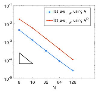
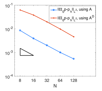
(a)	(b)

Figure 6.1: Reduction of the (a) displacement and (b) pressure errors for different mesh-sizes, by using the enriched finite element scheme, $\mathcal{A}$ (23), as well as the scheme with diagonal block used for the bubble functions, $\mathcal{A}^{D}$ (39).

6.2 Stokes’ problem

While it is well-known that the P1-P0 finite element pair is not stable for Stokes’ equations, we show here that the new formulation, $\widehat{\mathcal{A}}^{D}_{S}$ (63), resulting from the elimination of the normal components of the bubbles, does provides a stable method. Consider (54)-(56) on a unit square $(0,1)\times(0,1)$, where the right-hand side ${\bm{f}}$ is chosen such that the analytical solution is given by

$${\bm{u}}(x,y)=\left(\sin(\pi x)\cos(\pi y),-\cos(\pi x)\sin(\pi y)\right),\quad p(x,y)=0.5-x.$$

Figure 6.2 compares the error reduction for both the velocity and pressure using the bubble function enhanced schemes described by $\mathcal{A}_{S}$ (61) and $\mathcal{A}_{S}^{D}$ (62).

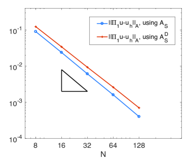
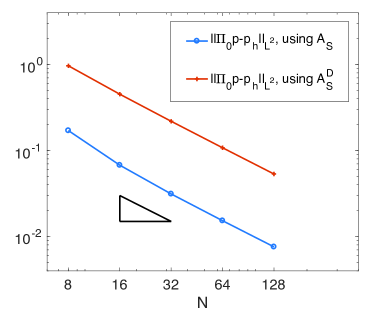
(a)	(b)

Figure 6.2: Reduction of the (a) velocity and (b) pressure errors for different mesh-sizes, by using the enriched finite element scheme, $\mathcal{A}_{S}$ (61), as well as the scheme resulting from using a diagonal block for the bubble functions, $\mathcal{A}^{D}_{S}$ (62).

Here, for the scheme $\mathcal{A}_{S}$ (61), the energy norm for the velocity is defined as $\|\bm{v}\|_{A}^{2}:=a^{S}(\bm{v},\bm{v})=2\mu({\bm{\varepsilon}}(\bm{v}),{\bm{\varepsilon}}(\bm{v}))$ for $\bm{v}\in\bm{V}$ . In addition, for the scheme $\widehat{\mathcal{A}}_{S}^{D}$ (62), the energy norm is defined as $\|\bm{v}\|_{A}^{2}:=a^{S,D}(\bm{v},\bm{v})$ where $a^{S,D}(\bm{u},\bm{v})$ is defined as in (29) with $a(\cdot,\cdot)$ replaced by $a^{S}(\cdot,\cdot)$. Both methods give the same, optimal, order of convergence, demonstrating that the inclusion of the bubble functions guarantee the stability of the method. Moreover, though the errors are slightly higher, the elimination of the bubble functions would provide a stable convergent method, but reduces the problem to one that contains the same number of degrees of freedom as the P1-P0 discretization. Thus, we get a stable scheme with no increase in cost.

7 Conclusions

In this paper, we have shown how to stabilize the popular P1-RT0-P0 finite-element discretization for a three-field formulation of the poroelasticity problem. By adding the normal components of the bubble basis functions associated with the faces of the triangulation to the P1 element for displacements, we have demonstrated that an inf-sup condition is satisfied independently of the physical and discretization parameters of the problem. Moreover, the degrees of freedom added to the faces are eliminated resulting in a stable scheme with the same number of unknowns as in the initial P1-RT0-P0 discretization. Furthermore, this idea has been extended to the Stokes’ equations, yielding a stable finite-element formulation with the lowest possible number of degrees of freedom, equivalent to a P1-P0 discretization. Future work includes investigating such formulations and their performance for various applications in poroelasticity, and extending the discretization to other PDE systems which have simliar properties to the Stokes’ equations.

References

- [1] K. Terzaghi, Theoretical Soil Mechanics, Wiley: New York, 1943.
- [2] M. A. Biot, General theory of three-dimensional consolidation, Journal of Applied Physics 12 (2) (1941) 155–164.
- [3] M. A. Biot, Theory of elasticity and consolidation for a porous anisotropic solid, Journal of Applied Physics 26 (2) (1955) 182–185.
- [4] R. Showalter, Diffusion in poro-elastic media, Journal of Mathematical Analysis and Applications 251 (1) (2000) 310 – 340.
- [5] A. Ženíšek, The existence and uniqueness theorem in Biot’s consolidation theory, Apl. Mat. 29 (3) (1984) 194–211.
- [6] F. J. Gaspar, F. J. Lisbona, P. N. Vabishchevich, A finite difference analysis of Biot’s consolidation model, Appl. Numer. Math. 44 (4) (2003) 487–506. doi:10.1016/S0168-9274(02)00190-3.
- [7] F. J. Gaspar, F. J. Lisbona, P. N. Vabishchevich, Staggered grid discretizations for the quasi-static Biot’s consolidation problem, Appl. Numer. Math. 56 (6) (2006) 888–898. doi:10.1016/j.apnum.2005.07.002.
- [8] J. M. Nordbotten, Stable cell-centered finite volume discretization for Biot equations, SIAM Journal on Numerical Analysis 54 (2) (2016) 942–968.
- [9] R. Lewis, B. Schrefler, The Finite Element Method in the Static and Dynamic Deformation and Consolidation of Porous Media, Wiley: New York, 1998.
- [10] M. A. Murad, A. F. D. Loula, Improved accuracy in finite element analysis of Biot’s consolidation problem, Comput. Methods Appl. Mech. Engrg. 95 (3) (1992) 359–382. doi:10.1016/0045-7825(92)90193-N.
- [11] M. A. Murad, A. F. D. Loula, On stability and convergence of finite element approximations of Biot’s consolidation problem, Internat. J. Numer. Methods Engrg. 37 (4) (1994) 645–667. doi:10.1002/nme.1620370407.
- [12] M. A. Murad, V. Thomée, A. F. D. Loula, Asymptotic behavior of semidiscrete finite-element approximations of Biot’s consolidation problem, SIAM J. Numer. Anal. 33 (3) (1996) 1065–1083. doi:10.1137/0733052.
- [13] C. Rodrigo, F. Gaspar, X. Hu, L. Zikatanov, Stability and monotonicity for some discretizations of the Biot’s consolidation model, Computer Methods in Applied Mechanics and Engineering 298 (2016) 183–204.
- [14] X. Hu, C. Rodrigo, F. J. Gaspar, L. T. Zikatanov, A nonconforming finite element method for the Biot’s consolidation model in poroelasticity, Journal of Computational and Applied Mathematics 310 (2017) 143 – 154. doi:http://doi.org/10.1016/j.cam.2016.06.003.
- [15] J. J. Lee, Robust error analysis of coupled mixed methods for Biot’s consolidation model, Journal of Scientific Computing 69 (2) (2016) 610–632.
- [16] Q. Hong, J. Kraus, Parameter-robust stability of classical three-field formulation of Biot’s consolidation model, Submitted, preprint available in arXiv/1706.00724v1.
- [17] P. Phillips, M. Wheeler, A coupling of mixed and continuous Galerkin finite element methods for poroelasticity I: the continuous in time case, Computational Geosciences 11 (2) (2007) 131–144. doi:10.1007/s10596-007-9045-y.
- [18] P. Phillips, M. Wheeler, A coupling of mixed and continuous Galerkin finite element methods for poroelasticity II: the discrete-in-time case, Computational Geosciences 11 (2) (2007) 145–158. doi:10.1007/s10596-007-9044-z.
- [19] P. Phillips, M. Wheeler, A coupling of mixed and discontinuous Galerkin finite-element methods for poroelasticity, Computational Geosciences 12 (4) (2008) 417–435. doi:10.1007/s10596-008-9082-1.
- [20] N. Castelleto, J. A. White, M. Ferronato, Scalable algorithms for three-field mixed finite element coupled poromechanics, Journal of Computational Physics 327 (2016) 894 – 918.
- [21] M. Bause, F. Radu, U. Kocher, Space-time finite element approximation of the Biot poroelasticity system with iterative coupling, Computer Methods in Applied Mechanics and Engineering 320 (2017) 745 – 768. doi:http://doi.org/10.1016/j.cma.2017.03.017.
- [22] T. Almani, K. Kumar, A. Dogru, G. Singh, M. Wheeler, Convergence analysis of multirate fixed-stress split iterative schemes for coupling flow with geomechanics, Comput. Methods Appl. Mech. Engrg. 311 (1) (2016) 180 – 207.
- [23] K. Lipnikov, Numerical methods for the Biot model in poroelasticity, Ph.D. thesis, University of Houston (2002).
- [24] F. Brezzi, M. Fortin, Mixed and hybrid finite element methods, Vol. 15 of Springer Series in Computational Mathematics, Springer-Verlag, New York, 1991. doi:10.1007/978-1-4612-3172-1.
- [25] D. Boffi, F. Brezzi, L. F. Demkowicz, R. G. Durán, R. S. Falk, M. Fortin, Mixed finite elements, compatibility conditions, and applications, Vol. 1939 of Lecture Notes in Mathematics, Springer-Verlag, Berlin; Fondazione C.I.M.E., Florence, 2008, Lectures given at the C.I.M.E. Summer School held in Cetraro, June 26–July 1, 2006, Edited by Boffi and Lucia Gastaldi. doi:10.1007/978-3-540-78319-0.
- [26] D. Boffi, F. Brezzi, M. Fortin, Mixed finite element methods and applications, Vol. 44 of Springer Series in Computational Mathematics, Springer, Heidelberg, 2013. doi:10.1007/978-3-642-36519-5.
- [27] V. Girault, P.-A. Raviart, Finite element methods for Navier-Stokes equations, Vol. 5 of Springer Series in Computational Mathematics, Springer-Verlag, Berlin, 1986, Theory and algorithms. doi:10.1007/978-3-642-61623-5.
- [28] X. Hu, C. Rodrigo, F. J. Gaspar, L. T. Zikatanov, A nonconforming finite element method for the Biot’s consolidation model in poroelasticity, Journal of Computational and Applied Mathematics 310 (2017) 143–154. doi:10.1016/j.cam.2016.06.003.
- [29] A. Korn, Solution general du probleme d’equilibre dans la theorie de l’elasticite, Annales de la Faculte de Sciences de Toulouse 10 (1908) 705–724.
- [30] A. Korn, Ueber einige ungleichungen, welche in der theorie der elastischen und elektrischen schwingungen eine rolle spielen, Bulletin internationale de l’Academie de Sciences de Cracovie, 9 (1909) 705–724.
- [31] V. A. Kondratiev, O. A. Oleinik, On Korn’s inequalities, C. R. Acad. Sci. Paris Sér. I Math. 308 (16) (1989) 483–487. doi:10.1070/RM1989v044n06ABEH002297.
- [32] V. A. Kondratiev, O. A. Oleinik, Dependence of the constants in the Korn inequality on parameters that characterize the geometry of the domain, Uspekhi Mat. Nauk 44 (6(270)) (1989) 157–158. doi:10.1070/RM1989v044n06ABEH002297.
- [33] P. G. Ciarlet, The finite element method for elliptic problems, North-Holland Publishing Co., Amsterdam-New York-Oxford, 1978, Studies in Mathematics and its Applications, Vol. 4.
- [34] V. Thomée, Galerkin finite element methods for parabolic problems, 2nd Edition, Vol. 25 of Springer Series in Computational Mathematics, Springer-Verlag, Berlin, 2006.