1 Introduction

For most modern internet companies, wherever there is a metric that can be measured (e.g., time spent on a page, click-through rates, conversion of curiousity to a sale), there is almost always a randomized trial behind the scenes, with the goal of identifying an alternative website design that provides improvements over the default design. The use of such data-driven decisions for perpetual improvement is colloquially known as A/B testing in the case of two alternatives, or A/B/n testing for several alternatives. Given a default configuration and several alternatives (e.g., color schemes of a website), the standard practice is to divert a small amount of scientist-traffic to a randomized trial over these alternatives and record the desired metric for each of them. If an alternative appears to be significantly better, it is implemented; otherwise, the default setting is maintained.

At first glance, this procedure seems intuitive and simple. However, in cases where the aim is to optimize over one particular metric, this common tool suffers from several downsides. (1) First, whereas some alternatives may be clearly worse than the default, others may only have a slight edge. If one wishes to minimize the amount of time and resources spent on this randomized trial the more promising alternatives should intuitively get a larger share of the traffic than the clearly-worse alternatives. Yet typical A/B/n testing frameworks allocate traffic uniformly over alternatives. (2) Second, companies often desire to continuously monitor an ongoing A/B test as they may adjust their termination criteria as time goes by and possibly stop earlier or later than originally intended. However, just as if you flip a coin long enough, a long string of heads is eventually inevitable, the practice of continuous monitoring (without mathematically correcting for it) can easily fool the tester to believe that a result is statistically significant, when in reality it is not. This is one of the reasons for the lack of reproducibility of scientific results, an issue recently receiving increased attention from the public media. (3) Third, the lack of sufficient evidence or an insignificant improvement of the metric may make it undesirable from a practical or financial perspective to replace the default. Therefore, when a company runs hundreds to thousands of A/B tests within a year, ideally the number of statistically insignificant changes that it made should be small compared to the total number of changes made. Controlling the false alarm rate of each individual test at a desired level $\alpha$ however does not achieve this type of control, also known as controlling the false discovery rate. Of course, it is also desirable to detect better alternatives (when they exist), and to do so as quickly as possible.

In this paper, we provide a novel framework that addresses the above shortcomings of A/B or A/B/n testing. The first concern is tackled by employing recent advances in adaptive sampling like the pure-exploration multi-armed bandit (MAB) algorithm. For the second concern, we adopt the notion of any-time $p$-values for guilt-free continuous monitoring, and we make the advantages and risks of early-stopping transparent. Finally, we handle the third issue using recent advances in online false discovery rate (FDR) control. Hence the combined framework can be described as doubly-sequential (sequences of MAB tests, each of which is itself sequential). Although each of those problems has been studied in hitherto disparate communities, how to leverage the best of all worlds, if at all possible, has remained an open problem. The main contributions of this paper are in merging these ideas in a combined framework and presenting the conditions under which it can be shown to yield near-optimal sample complexity, near-optimal best-alternative discovery rate, as well as FDR control.

While the above concerns raised about A/B/n testing were discussed using the example of modern internet companies, the same concerns carry forward qualitatively to other domains, like pharmaceutical companies running sequential clinical trials with a control (often placebo) and a few treatments (like different doses or drug substances). In a manufacturing or food production setting, one may be interested in identifying (perhaps cheaper) substitutes for individual materials without compromising the quality of a product too much. In a government setting, pilot programs are funded in search of improvements over current programs and it is desirable from a social welfare standpoint and cost to limit the adoption of ineffective policies.

The remainder of this paper is organized as follows. In Section 2, we lay out the primary goals of the paper, and describe a meta-algorithm that combines adaptive sampling strategies with FDR control procedures. Section 3 is devoted to the description of a concrete procedure, along with some theoretical guarantees on its properties. In Section 4, we describe the results of our extensive experiments on both simulated and real-world data sets that are available to us, before we conclude with a discussion in Section 6.

2 Formal experimental setup and a meta-algorithm

In this section we first formalize the setup of a typical A/B/n test and provide a high-level overview of our proposed combined framework aimed at addressing the shortcomings mentioned in the introduction. A specific instantiation of this meta-algorithm along with detailed theoretical guarantees are specified in Section 3.

For concreteness, we refer to the system designer, whether a tech company or a pharmaceutical company, as a (data) scientist. We assume that the scientist needs to possibly conduct an infinite number of experiments sequentially, indexed by $j$. Each experiment has one default setting, referred to as the control, and $K=K(j)$ alternative settings, called the treatments or alternatives. The scientist must return one of the $K+1$ options that is the “best” according to some predefined metric, before the next experiment is started. Such a setup is a simple mathematical model both for clinical trials run by pharmaceutical labs, and A/B/n testing used at scale by tech companies.

One full experiment consists of steps of the following kind: In each step, the scientist assigns a new person—who arrives at the website or who enrolls in the clinical trial—to one of the $K+1$ options and obtains a measurable outcome. In practice, the role of the scientist could be taken by an adaptive algorithm, which determines the assignment at time step $j$ by careful consideration of all previous outcomes. Borrowing terminology from the multi-armed bandit (MAB) literature, we refer to each of the $K+1$ options as an arm, and each assignment to arm $i$ is termed “pulling arm $i$”. For concreteness, we assign the index $0$ to the default or control arm, and note that this index is known to the algorithm.

We assume that the observable metric from each pull of arm $i=0,1,\dots,K$ corresponds to an independent draw from an unknown probability distribution with expectation $\mu_{i}$. Ideally, if the means were known, we would use them as scores to compare the arms where higher is better. In the sequel we use $\mu_{i_{\star}}:=\max\limits_{i=1,\dots,K}\mu_{i}$ to denote the mean of the best arm. We refer the reader to Table 1 for a glossary of the notation used throughout this paper.

2.1 Some desiderata and difficulties

Given the setup above, how can we mathematically describe the guarantees that the companies might desire from an improved multiple-A/B/n testing framework? Which parts of the puzzle can be directly transferred from known results, and what challenges remain?

In order to answer the first question, let us adopt terminology from the hypothesis testing literature and view each experiment as a test of a null hypothesis. Any claim that an alternative arm is the best is called a discovery, and if such a claim is erroneous then it is called a false discovery. When multiple hypotheses need to be tested, the scientist needs to define the quantity it wants to control. While we may desire that the probability of even a single false discovery—called the family-wise error rate—is small, this is usually far too stringent for a large and unknown number of tests. For this reason, [1] proposed that it may be more interesting to control the expected ratio of false discoveries to the total number of discoveries (called the False Discovery Rate, or FDR for short) or ratio of expected number of false discoveries to the expected number of total discoveries (called the modified FDR or mFDR for short). Over the past decades, the FDR and its variants like mFDR have become standard quantities for multiple testing applications. In the following, if not otherwise specified, we use the term FDR to denote both measures in order to simplify the presentation. In Section 3, we show that both mFDR and FDR can be controlled for different choices of procedures.

2.1.1 Challenges in viewing an MAB instance as a hypothesis test

In our setup, we want to be able to control the FDR at any time in an online manner. Online FDR procedures were first introduced by Foster and Stine [2], and have since been studied by other authors (e.g., [3, 4]). A typical online FDR procedure is based on comparing a valid $p$-value $P^{j}$ with carefully-chosen levels $\alpha_{j}$ for each hypothesis test. We reject the null hypothesis, represented as $R_{j}=1$, when $P^{j}\leq\alpha_{j}$ and we set $R_{j}=0$ otherwise.

As mentioned, we want to use adaptive MAB algorithms in each experiment to test each hypothesis, since they can find a best arm among $K+1$ with near-optimal sample complexity. However the traditional MAB setup does not account for the asymmetry between the arms as is the case in a testing setup, with one being the default (control) and others being alternatives (treatments). This is the standard scenario in A/B/n testing applications, as for example a company might prefer wrong claims that the control is the best (false negative), rather than wrong claims that an alternative is the best (false positive), simply because new system-wide adoption of selected alternatives might involve high costs. What would be a suitable null hypothesis in this hybrid setting? To allow continuous monitoring, is it possible to define and compute always-valid $p$-values that are super-uniformly distributed under the null hypothesis when computed at any time $t$? (This could be especially challenging given that the number of samples from each the arm is random, and different for each arm.)

In addition to asymmetry, the practical scientist might have a different incentive than the ideal outcome for MAB algorithms. In particular, he/she might not want to find the best alternative if it is not substantially better than the control. Indeed, if the net gain made by adopting a new alternative is small, it might be offset by the cost of implementing the change from the existing default choice. By similar reasoning, we may not require identifying the single best arm if there is a set of arms with similar means that are all larger than the rest.

We propose a sensible null-hypothesis for each experiment which incorporates the approximation and improvement notions as described above and provide an always valid $p$-value which can be easily calculated at each time step in the experiment. We show that a slight modification of the usual LUCB algorithm caters to this specific null-hypothesis while still maintaining near-optimal sample complexity.

2.1.2 Interaction between MAB and FDR

In order to take advantage of the sample efficiency of best-arm bandit algorithms, it is crucial to set the confidence levels close to what is needed. Given a user-defined level $\alpha$, at each hypothesis $j$, online FDR procedures automatically output the significance level $\alpha_{j}$ which are “needed” to guarantee FDR control, based on past decisions.

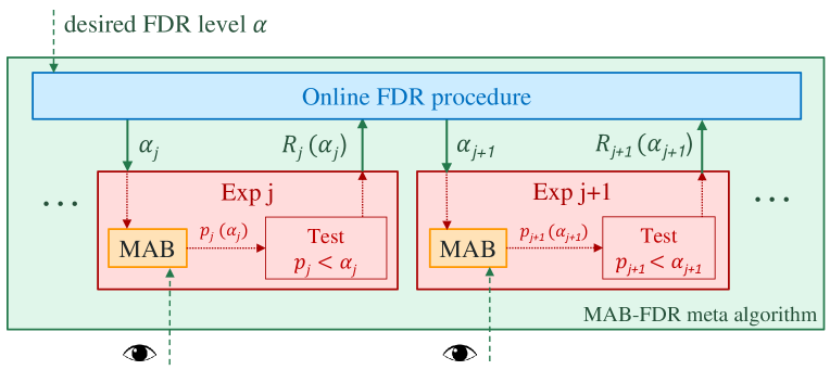
Figure 1: Diagram of the MAB-FDR meta algorithm designed to achieve online FDR control along with near-optimal sample complexity. The green arrows symbolize interaction between the MAB and FDR procedures via the FDR test levels $\alpha_{j}$ and rejection indicator variables $R_{j}$. Notice that the $P^{j}$-values are now dependent as each $\alpha_{j}$ depends on $R_{1},\dots,R_{j-1}$. The eyes represent possible continuous monitoring by the scientist.

Can we directly set the MAB confidence levels to the output levels $\alpha_{j}$ from the online FDR procedure? If we do, our $p$-values are not independent across different hypotheses anymore: $P^{j}$ directly depends on the FDR levels $\alpha_{j}$ and each $\alpha_{j}$ in turn depends on past MAB rejections, thus on past MAB $p$-values (see Figure 1). Does the new interaction compromise FDR guarantees?

Although known online FDR procedures [2, 4] guarantee FDR control for independent $p$-values, this does not hold for dependent $p$-values in general. Hence FDR control guarantees cannot simply be obtained out of the box. In particular, it is not a priori obvious that the introduced dependence between the $p$-values does not cause problems, i.e. violates necessary conditions for FDR control type theorems. A key insight that emerges from our analysis is that an appropriate bandit algorithm actually shapes the $p$-value distribution under the null in a “good” way that allows us to control FDR.

2.2 A meta-algorithm

Procedure 1 summarizes our doubly-sequential procedure, with a corresponding flowchart in Figure 1. We will prove theoretical guarantees after instantiating the separate modules. Note that our framework allows the scientist to plug in their favorite best-arm MAB algorithm or online FDR procedure. The choice for each of them determines which guarantees can be proven for the entire setup. Any independent improvement in either of the two parts would immediately lead to an overall performance boost of the overall framework.

Procedure 1 MAB-FDR Meta algorithm skeleton

1. The scientist sets a desired FDR control rate $\alpha$.

2. For each $j=1,2,\dots$:

   • Experiment $j$ receives a designated control arm and some number of alternative arms.

   • An online-FDR procedure returns an $\alpha_{j}$ that is some function of the past values $\{P^{\ell}\}_{\ell=1}^{j-1}$.

   • An MAB procedure with inputs (a) the control arm and $K(j)$ alternative arms, (b) confidence level $\alpha_{j}$, and (c) (optional) a precision $\epsilon\geq 0$, is executed and if the procedure self-terminates, returns a recommended arm.

   • Throughout the MAB procedure, an always valid $p$-value is constructed continuously for each time $t$ using only the samples collected up to that time from the $j$-th experiment: for any $t$, it is a random variable $P^{j}_{t}\in[0,1]$ that is super-uniformly distributed whenever the control-arm is best.

   • When the MAB procedure is terminated at time $t$ (either by itself or by a user-defined stopping criterion that may depend on $P^{j}_{t}$), if the arm with the highest empirical mean is not the control arm and $P^{j}_{t}\leq\alpha_{j}$, then we return $P^{j}:=P^{j}_{t}$, and the control arm is rejected in favor of this empirically best arm.

3 A concrete procedure with guarantees

We now take the high-level road map given in Procedure 1, and show that we can obtain a concrete, practically implementable framework with FDR control and power guarantees. We first discuss the key modeling decisions we have to make in order to seamlessly embed MAB algorithms into an online FDR framework. We then outline a modified version of a commonly used best-arm algorithm, before we finally prove FDR and power guarantees for the concrete combined procedure.

3.1 Defining null hypotheses and constructing $p$-values

Our first task is to define a null hypothesis for each experiment. As mentioned before, the choice of the null is not immediately obvious, since we sample from multiple distributions adaptively instead of independently. In particular, we will generally not have the same number of samples for all arms. Given a distribution with default mean $\mu_{0}$ and alternative distributions with means $\{\mu_{i}\}_{i=1}^{K}$, we propose that the null hypothesis for the $j$-th experiment should be defined as

$$H_{0}^{j}:\mu_{0}\geq\mu_{i}-\epsilon\quad\mbox{for all $i=1,\dots,K$.}$$ (1)

In words, the null corresponds to there being no alternative arm that is $\epsilon$-better than the control arm.

It remains to define a $p$-value for each experiment that is stochastically dominated by a uniform random variable under the null; such a $p$-value is said to be superuniform. In order to simplify notation below, we omit the index $j$ for the experiment and retain only the index $i$ for the choice of arms. In order to be able to use a $p$-value at arbitrary times in the testing procedure and to allow scientists to monitor the algorithm’s progress in real time, it is helpful to define an always valid $p$-value, as previously defined by Johari et al. [5]. An always valid p-value is a stochastic process $\{P_{t}\}_{t=1}^{\infty}$ such that for all fixed and random stopping times $T$, under any distribution $\mathbb{P}_{0}$ over the arm rewards such that the null hypothesis is true, we have

$$\mathbb{P}_{0}(P_{T}\leq\alpha) \leq\alpha.$$ (2)

When all arms are drawn independently an equal number of times, by linearity of expectation one can regard the distance of each pair of samples as a random variable drawn i.i.d. from a distribution with mean $\tilde{\mu}_{i}:=\mu_{0}-\mu_{i}$. We can then view the problem as testing the standard hypothesis $H_{0}:\tilde{\mu}_{i}>-\epsilon$. However, when the arms are pulled adaptively, a different solution needs to be found—indeed, in this case, the sample means are not unbiased estimators of the true means, since the number of times an arm was pulled now depends on the empirical means of all the arms.

Our strategy is to construct always valid $p$-values by using the fact that p-values can be obtained by inverting confidence intervals. To construct always-valid confidence bounds, we resort to the fundamental concept of the law of the iterated logarithm (LIL), for which non-asymptotic versions have been recently derived and used for both bandits and testing problems (see [6], [7]).

To elaborate, define the function

$$\varphi_{n}(\delta)=\sqrt{\frac{\log(\frac{1}{\delta})+3\log(\log(\frac{1}{\delta}))+\frac{3}{2}\log(\log(\mathrm{e}n))}{n}}.$$ (3)

If $\widehat{\mu}_{i,n}$ is the empirical average of independent samples from a sub-Gaussian distribution, then it is known (see, for instance,  [8, Theorem 8]) that for all $\delta\in(0,1)$, we have

$$\max\Big{\{} \mathbb{P}\Big{(}\bigcup_{n=1}^{\infty}\{\widehat{\mu}_{i,n}-\mu_{i}>\varphi_{n}(\delta\wedge 0.1)\}\Big{)},\quad\mathbb{P}\Big{(}\bigcup_{n=1}^{\infty}\{\widehat{\mu}_{i,n}-\mu_{i}<-\varphi_{n}(\delta\wedge 0.1)\}\Big{)}\Big{\}}\leq\delta,$$ (4)

where $\delta\wedge 0.1:=\min\{\delta,0.1\}$.

We are now ready to propose single arm $p$-values of the form

$$P_{i,t}: =\sup\Big{\{}\gamma\in[0,1]\;\mid\;\>\widehat{\mu}_{i,n_{i}(t)}-\varphi_{n_{i}(t)}(\tfrac{\gamma}{2K})\leq\>\widehat{\mu}_{0,n_{0}(t)}+\varphi_{n_{0}(t)}(\tfrac{\gamma}{2})+\epsilon\Big{\}}$$ (5)

$$=\sup\Big{\{}\gamma\in[0,1]\;\mid\;\text{LCB}_{i}(t)\leq\text{UCB}_{0}(t)+\epsilon\Big{\}}$$

Here we set $P_{i,t}=1$ if the supremum is taken over an empty set. Given these single arm $p$-values, the always-valid $p$-value for the experiment is defined as

$$P_{t} :=\min_{s\leq t}\;\min_{i=1,\ldots,K}P_{i,s}.$$ (6)

We claim that this procedure leads to an always valid $p$-value (with proof in Appendix 5.1).

Proposition 1.

The sequence $\{P_{t}\}_{t=1}^{\infty}$ defined via equation (6) is an always valid $p$-value.

See Section 5.1 for the proof of this proposition.

3.2 Adaptive sampling for best-arm identification

In the traditional A/B testing setting described in the introduction, samples are allocated uniformly to the different alternatives. But by allocating different numbers of samples to the alternatives, decisions can be made with the same statistical significance using far fewer samples. Suppose moreover that there is a unique maximizer $i_{\star}:=\arg\max\limits_{i=0,1,\dots,K}\mu_{i}$, so that

$$\Delta_{i}:=\mu_{i_{\star}}-\mu_{i}>0\qquad\mbox{for all $i\neq i_{\star}$.}$$

Then for any $\delta\in(0,1)$, best-arm identification algorithms for the multi-armed bandit problem can identify $i_{\star}$ with probability at least $1-\delta$ based on at most $\sum_{i\neq i_{\star}}\Delta_{i}^{-2}\log(1/\delta)$ total samples (see the paper [9] for a brief survey and [10] for an application to clinical trials). In contrast, if samples are allocated uniformly to the alternatives under the same conditions, then the most natural procedures require $K\max\limits_{i\neq i_{\star}}\Delta_{i}^{-2}\log(K/\delta)$ samples before returning $i_{\star}$ with probability at least $1-\delta$.

However, standard best-arm bandit algorithms do not incorporate asymmetry as induced by null-hypotheses as in definition (1) by default. Furthermore, recall that a practical scientist might desire the ability to incorporate approximation and a minimum improvement requirement. More precisely, it is natural to consider the requirement that the returned arm $i_{b}$ satisfies the bounds $\mu_{i_{b}}\geq\mu_{0}+\epsilon$ and $\mu_{i_{b}}\geq\mu_{i_{\star}}-\epsilon$ for some $\epsilon>0$. For those readers unfamiliar with best-arm MAB algorithms, it is likely helpful to first grasp the entire framework in the special $\epsilon=0$ throughout, before understanding it in full generality with the complications introduced by setting $\epsilon>0$. In the following we present a modified MAB algorithm based on the common LUCB algorithm (see [11, 12]).

Algorithm 1 Best-arm identification with a control arm for confidence $\delta$ and precision $\epsilon\geq 0$

For all $t$ let $n_{i}(t)$ be the number of times arm $i$ has been pulled up to time $t$. In addition, for each arm $i$ let $\widehat{\mu}_{i}(t)=\frac{1}{n_{i}(t)}\sum_{\tau=1}^{n_{i}(t)}r_{i}(\tau)$, define

$$\text{LCB}_{i}(t) :=\widehat{\mu}_{i,n_{i}(t)}-\varphi_{n_{i}(t)}(\tfrac{\delta}{2K})\qquad\mbox{and}\qquad\text{UCB}_{i}(t):=\widehat{\mu}_{i,n_{i}(t)}+\varphi_{n_{i}(t)}(\tfrac{\delta}{2}).$$

1. Set $t=1$ and sample every arm once.

2. Repeat: Compute $h_{t}=\arg\max\limits_{i=0,1,\dots,K}\widehat{\mu}_{i}(t)$, and $\ell_{t}=\arg\max\limits_{i=0,1,\dots,K,i\neq h_{t}}\text{UCB}_{i}(t)$

   1. If $\text{LCB}_{0}(t)>\text{UCB}_{i}(t)-\epsilon$, for all $i\neq 0$, then output $0$ and terminate.
      Else if $\text{LCB}_{h_{t}}(t)>\text{UCB}_{\ell_{t}}(t)-\epsilon$ and $\text{LCB}_{h_{t}}(t)>\text{UCB}_{0}(t)+\epsilon$, then output $h_{t}$ and terminate.

   2. If $\epsilon>0$, let $u_{t}=\arg\max_{i\neq 0}\text{UCB}_{i}(t)$ and pull all distinct arms in $\{0,u_{t},h_{t},\ell_{t}\}$ once.
      If $\epsilon=0$, pull arms $h_{t}$ and $\ell_{t}$ and set $t=t+1$.

Inside the loop of Algorithm 1, we use $h_{t}\in\{0,1,\dots,K\}$ to denote the current empirically-best arm, $\ell_{t}$ to denote the most promising contender among the other arms that has not yet been sampled enough to be ruled out. The parameter $\epsilon\geq 0$ is a slack variable, and the algorithm is easiest to first understand when $\epsilon=0$. We provide a visualization of how $\epsilon$ affects the stopping condition in Figure 2. Step (a) checks if $h_{t}$ is within $\epsilon$ of the true highest mean, and if it is also at least $\epsilon$ greater than the true mean of the control arm (or is the control arm), terminates with this arm $h_{t}$. Step (b) ensures that the control arm is sufficiently sampled when $\epsilon>0$. Step (c) pulls $h_{t}$ and $\ell_{t}$, reducing the overall uncertainty in the difference between their two means.

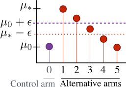
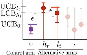
(a)	(b)

Figure 2: (a) The means of arms $\{1,2,3\}$ are within $\epsilon$ of the best arm, but only arms $\{1,2\}$ are at least $\epsilon$ better than the control arm 0. Thus, returning any of arms $\{3,4,5\}$ would result in a false discovery when $\epsilon>0$. (b) An example of the stopping condition being critically met and returning a non-control arm $h_{t}$. While $\text{LCB}_{h_{t}}>\text{UCB}_{\ell_{t}}-\epsilon$ is satisfied with some slack, $\text{LCB}_{h_{t}}>\text{UCB}_{0}+\epsilon$ is just barely satisfied.

The following proposition applies to Algorithm 1 run with a control arm indexed by $i=0$ with mean $\mu_{0}$ and alternative arms indexed by $i=1,\dots,K$ with means $\mu_{i}$, respectively. Let $i_{b}$ denote the random arm returned by the algorithm assuming that it exits, and define the set

$$\mathcal{S}^{\star} :=\{i_{\star}\neq 0\mid\mu_{i_{\star}}\geq\max\limits_{i=1,\dots,K}\mu_{i}-\epsilon\quad\mbox{and}\quad\mu_{i_{\star}}>\mu_{0}+\epsilon\}.$$ (7)

Note that the mean associated with any index $i_{\star}\in\mathcal{S}^{\star}$, assuming that the set is non-empty, is guaranteed to be $\epsilon$-superior to the control mean, and at most $\epsilon$-inferior to the maximum mean over all arms.

Proposition 2.

The algorithm 1 terminates in finite time with probability one. Furthermore, suppose that the samples from each arm are independent and sub-Gaussian with scale $1$. Then for any $\delta\in(0,1)$ and $\epsilon\geq 0$, Algorithm 1 has the following guarantees:

1. Suppose that $\mu_{0}>\max\limits_{i=1,\dots,K}\mu_{i}-\epsilon$. Then with probability at least $1-\delta$, the algorithm exits with $i_{b}=0$ after taking at most $O\left(\sum_{i=0}^{K}\widetilde{\Delta}_{i}^{-2}\log(K\log(\widetilde{\Delta}_{i}^{-2})/\delta)\right)$ time steps with effective gaps

   $$\widetilde{\Delta}_{0} =(\mu_{0}+\epsilon)-\max\limits_{j=1,\dots,K}\mu_{j}\>\text{ and}$$

   $$\widetilde{\Delta}_{i} =(\mu_{0}+\epsilon)-\mu_{i}.$$

2. Otherwise, suppose that the set $\mathcal{S}^{\star}$ as defined in equation (7) is non-empty. Then with probability at least $1-\delta$, the algorithm exits with $i_{b}\in\mathcal{S}^{\star}$ after taking at most
   $O\left(\sum_{i=0}^{K}\widetilde{\Delta}_{i}^{-2}\log(K\log(\widetilde{\Delta}_{i}^{-2})/\delta)\right)$ time steps with effective gaps

   $$\widetilde{\Delta}_{0} =\min\left\{\max\limits_{j=1,\dots,K}\mu_{j}-(\mu_{0}+\epsilon),\max\{\Delta_{0},\epsilon\}\right\}\>\text{ and}$$

   $$\widetilde{\Delta}_{i} =\max\left\{\Delta_{i},\min\left\{\max\limits_{j=1,\dots,K}\mu_{j}-(\mu_{0}+\epsilon),\epsilon\right\}\right\}.$$

See Section 5.2 for the proof of this claim. Part (a) of Proposition 2 guarantees that when no alternative arm is $\epsilon$-superior to the control arm (i.e. under the null hypothesis), the algorithm stops and returns the control arm after a certain number of samples with probability at least $1-\delta$, where the sample complexity depends on $\epsilon$-modified gaps between the means $\mu_{0}$ and $\mu_{i}$. Part (b) guarantees that if there is in fact at least one alternative that is $\epsilon$-superior to the control arm (i.e. under the alternative), then the algorithm will find at least one of them that is at most $\epsilon$-inferior to the best of all possible arms with the same sample complexity and probability.

Note that the required number of samples $O\left(\sum_{i=0}^{K}\widetilde{\Delta}_{i}^{-2}\log(K\log(\widetilde{\Delta}_{i}^{-2})/\delta)\right)$ in Proposition 2 is comparable, up to log factors, with the well-known results in [11, 12] for the case $\epsilon=0$, with the modified gaps $\widetilde{\Delta}_{i}$ replacing $\Delta_{i}=\mu_{i_{\star}}-\mu_{i}$. Indeed, the nearly optimal sample complexity result of [12] implies that the algorithm terminates under settings (a) and (b) after at most $O(\max_{j\neq i_{\star}}\Delta_{j}^{-2}\log(K\log(\Delta_{j}^{-2})/\delta)+\sum_{i\neq i_{\star}}\Delta_{i}^{-2}\log(\log(\Delta_{i}^{-2})/\delta)$) samples are taken.

In our development to follow, we now bring back the index for experiment $j$, in particular using $P^{j}$ to denote the quantity $P^{j}_{T}$ at any stopping time $T$. Here the stopping time can either be defined by the scientist, or in an algorithmic manner.

3.3 Best-arm MAB interacting with online FDR

After having established null hypotheses and $p$-values in the context of best-arm MAB algorithms, we are now ready to embed them into an online FDR procedure. In the following, we consider $p$-values for the $j$-th experiment $P^{j}:=P^{j}_{T_{j}}$ which is just the $p$-value as defined in equation (6) at the stopping time $T_{j}$, which depends on $\alpha_{j}$.

We denote the set of true null and false null hypotheses up to experiment $J$ as $\mathcal{H}_{0}(J)$ and $\mathcal{H}_{1}(J)$ respectively, where we drop the argument whenever it’s clear from the context. The variable $R_{j}=\mathbbm{1}_{P^{j}\leq\alpha_{j}}$ indicates whether a the null hypothesis of experiment $j$ has been rejected, where $R_{j}=1$ denotes a claimed discovery that an alternative was better than the control. The false discovery rate (FDR) and modified FDR up to experiment $J$ are then defined as

$$\text{FDR}(J) :=\mathbb{E}\frac{\sum_{j\in\mathcal{H}_{0}}R_{j}}{\sum_{i=1}^{J}R_{i}\vee 1}\qquad\text{ and }\qquad\text{mFDR}(J):=\frac{\mathbb{E}\sum_{j\in\mathcal{H}_{0}}R_{j}}{\mathbb{E}\sum_{i=1}^{J}R_{i}+1}.$$ (8)

Here the expectations are taken with respect to distributions of the arm pulls and the respective sampling algorithm. In general, it is not true that control of one quantity implies control of the other. Nevertheless, in the long run (when the law of large numbers is a good approximation), one does not expect a major difference between the two quantities in practice.

The set of true nulls $\mathcal{H}_{0}$ thus includes all experiments where $H_{0}^{j}$ is true, and the FDR and mFDR are well-defined for any number of experiments $J$, since we often desire to control $\text{FDR}(J)$ or $\text{mFDR}(J)$ for all $J\in\mathbb{N}$. In order to measure power, we define the $\epsilon$-best-arm discovery rate as

$$\epsilon\text{BDR}(J) :=\frac{\mathbb{E}\sum_{j\in\mathcal{H}_{1}}R_{j}\mathbbm{1}_{\mu_{i_{b}}\geq\mu_{i_{\star}}-\epsilon}\mathbbm{1}_{\mu_{i_{b}}\geq\mu_{0}+\epsilon}}{|\mathcal{H}_{1}(J)|}$$ (9)

We provide a concrete procedure 2 for our doubly sequential framework, where we use a particular online FDR algorithm due to Javanmard and Montanari [4] known as LORD; the reader should note that other online FDR procedure could be used to obtain essentially the same set of guarantees. Given a desired level $\alpha$, the LORD procedure starts off with an initial “$\alpha$-wealth” of $W(0)<\alpha$. Based on a inifinite sequence $\{\gamma_{i}\}_{i=1}^{\infty}$ that sums to one, and the time of the most recent discovery $\tau_{j}$, it uses up a fraction $\gamma_{j-\tau_{j}}$ of the remaining $\alpha$-wealth to test. Whenever there is a rejection, we increase the $\alpha$-wealth by $\alpha-W(0)$. A feasible choice for a stopping time in practice is $T_{j}:=\min\{T(\alpha_{j}),M\}$, where $M$ is a maximal number of samples the scientist wants to pull and $T(\alpha_{j})$ is the stopping time of the best-arm MAB algorithm run at confidence $\alpha_{j}$.

Procedure 2 MAB-LORD: best-arm identification with online FDR control

1. Initialize $W(0)<\alpha$, set $\tau_{0}=0$, and choose a sequence $\{\gamma_{i}\}$ s.t. $\sum_{i=1}^{\infty}\gamma_{i}=1$

2. At each step $j$, compute $\alpha_{j}=\gamma_{j-\tau_{j}}W(\tau_{j})$ and
   $W(j+1)=W(j)-\alpha_{j}+R_{j}(\alpha-W(0))$

3. Output $\alpha_{j}$ and run Algorithm 1 using $\alpha_{j}$-confidence and stop at a stopping time $T_{j}$.

4. Algorithm 1 returns $P^{j}$ and we reject the null hypothesis if $P^{j}\leq\alpha_{j}$.

5. Set $R_{j}=\mathbbm{1}_{P^{j}\leq\alpha_{j}},\tau_{j}=\tau_{j-1}\vee jR_{j}$, update $j=j+1$ and go back to step 2.

The following theorem provides guarantees on mFDR and power for the MAB-LORD procedure.

Theorem 1 (Online mFDR control for MAB-LORD).

1. Procedure 2 achieves mFDR control at level $\alpha$ for stopping times $T_{j}=\min\{T(\alpha_{j}),M\}$.

2. Furthermore, if we set $M=\infty$, Procedure 2 satisfies

   $$\epsilon\text{BDR}(J)\geq\frac{\sum_{j=1}^{J}\mathbbm{1}_{j\in\mathcal{H}_{1}}(1-\alpha_{j})}{|\mathcal{H}_{1}(J)|}.$$ (10)

The proof of this theorem can be found in Section 5.3. Note that by the arguments in the proof of Theorem 1, mFDR control itself is actually guaranteed for any generalized $\alpha$-investing procedure [3] combined with any best-arm MAB algorithm. In fact we could use any adaptive stopping time $T_{j}$ which depend on the history only via the rejections $R_{1},\dots,R_{j-1}$. Furthermore, using a modified LORD proposed by Javanmard and Montanari [13], we can also guarantee FDR control– which can be found in Appendix B.

It is noteworthy that small values of $\alpha$ do not only guarantee smaller FDR error but also higher BDR. However, there is no free lunch — a smaller $\alpha$ implies a smaller $\alpha_{j}$ at each experiment, which in turn causes the best-arm MAB algorithm to employ a larger number of pulls in each experiment.

4 Experimental results

In the following, we describe the results of experiments on both simulated and real-world data sets to illustrate the properties and guarantees of our procedure described in Section 3. In particular, we show that the mFDR is indeed controlled over time and that MAB-FDR (used interchangeably with MAB-LORD here) is highly advantageous in terms of sample complexity and power compared to a straightforward extension of A/B testing that is embedded in online FDR procedures. Unless otherwise noted, we set $\epsilon=0$ in all of our simulations to focus on the main ideas and keep the discussion concise.

There are two natural frameworks to compare against MAB-FDR. The first, called AB-FDR or AB-LORD, swaps the MAB part for an A/B (i.e. A/B/n) test (uniformly sampling all alternatives until termination). The second comparator swaps the online FDR control for independent testing at $\alpha$ for all hypotheses – we call this MAB-IND. Formally, AB-FDR swaps step 3 in Procedure 2 with “Output $\alpha_{j}$ and uniformly sample each arm until stopping time $T_{j}$.” while MAB-IND swaps step 4 in Procedure 2 with “The algorithm returns $P^{j}$ and we reject the null hypothesis if $P^{j}\leq\alpha$.”. In order to compare the performances of these procedures, we ran three sets of simulations using Procedure 2 with $\epsilon=0$ and $\gamma_{j}=0.07\>\frac{\log(j\vee 2)}{j\mathrm{e}^{\sqrt{\log j}}}$ as in [4]. The first two sets are on artificial data (Gaussian and Bernoulli draws from sets of randomly drawn means $\mu_{i}$), while the third is based on data from the New Yorker Cartoon Caption Contest (Bernoulli draws).

Our experiments are run on artificial data with Gaussian/Bernoulli draws and real-world Bernoulli draws from the New Yorker Cartoon Caption Contest. Recall that the sample complexity of the best-arm MAB algorithm is determined by the gaps $\Delta_{j}=\mu_{i_{\star}}-\mu_{j}$. One of the main relevant differences to consider between an experiment of artificial or real-world nature is thus the distribution of the means $\mu_{i}$ for $i=1,\dots,K$. The artificial data simulations are run with a fixed gap between the mean of the best arm $\mu_{i_{\star}}$ and second best arm $\mu_{2}$, which we denote by $\Delta=\mu_{i_{\star}}-\mu_{2}$. In each experiment (hypothesis), the means of the other arms are set uniformly in $[0,\mu_{2}]$. For our real-world simulations with the cartoon contest, the means for the arms in each experiment are not arbitrary but correspond to empirical means from the caption contest. In addition, the contests actually follow a natural chronological order (see details below), which makes this dataset highly relevant to our purposes. In all simulations, 60% of all the hypotheses are true nulls, and their indices are chosen uniformly.

4.1 Power and sample complexity

The first set of simulations compares MAB-FDR against AB-FDR. They confirm that the total number of necessary pulls to determine significance (which we refer to as sample complexity) is much smaller for MAB-FDR than for AB-FDR. In the MAB-FDR framework, this also effectively leads to higher power given a fixed truncation time.

Two types of plots are used to demonstrate the superiority of our procedure: for one we fix the number of arms and plot the $\epsilon\text{BDR}$ with $\epsilon=0$ (which we call BDR for short) for both procedures over different choices of truncation times $M$. For the other we fix $M$ and show how the sample complexity varies with the number of arms. Note that low BDR means that the bandit algorithm often reaches truncation time before it could stop.

4.1.1 Simulated Gaussian and Bernoulli trials

For the Gaussian draws, we set $\mu_{i_{\star}}=8$. The gap to the second best arm is $\Delta=3$ so that all means $\mu_{i\neq i_{\star}}$ are drawn uniformly between $Unif\sim[0,5]$. The number of hypotheses is fixed to be $500$. For Bernoulli draws we choose the maximum mean to be $\mu_{i_{\star}}=0.4$, $\Delta=0.3$ so that all means $\mu_{i\neq i_{\star}}$ are drawn uniformly between $Unif\sim[0,0.1]$. The number of hypotheses is fixed at $50$. We display the empirical average over $100$ runs where each run uses the same hypothesis sequence (indicating which hypotheses are true and false) and sequence of means $\mu_{i}$ for each hypothesis. The only randomness we average over comes from the random Gaussian/Bernoulli draws which cause different rejections $R_{j}$ and $\alpha_{j}$, so that the randomness in each draw propagates through the online FDR procedure. The results can be seen in Figures 3 and 4.

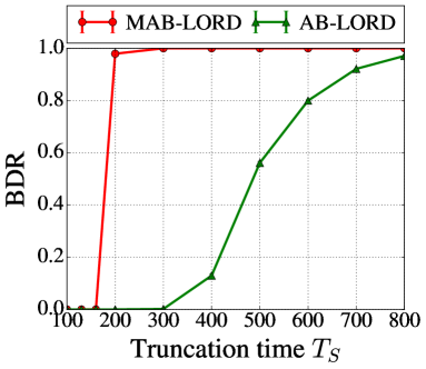
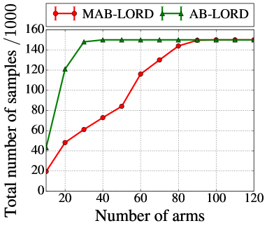
(a)	(b)

Figure 3: (a) Power vs. truncation time $T_{S}$ (per hypothesis) for $50$ arms and (b) Sample complexity vs. # arms for truncation time $M=300$ for Gaussian draws with fixed $\mu_{i_{\star}}=8$, $\Delta=3$ over $500$ hypotheses with $200$ non-nulls, averaged over $100$ runs.

The power at any given truncation time is much higher for MAB-FDR than AB-FDR. This is because the best-arm MAB is more likely to satisfy the stopping criterion before any given truncation time than the uniform sampling algorithm. The plot in Fig. 3(a) suggests that the actual stopping time of the algorithm is concentrated between $160$ and $200$ while it is much more spread out for the uniform algorithm.

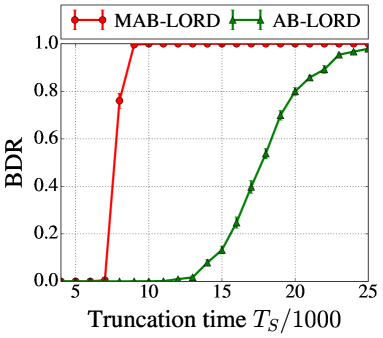
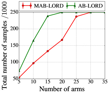
(a)	(b)

Figure 4: (a) Power over truncation time $T_{S}$ (per hypothesis) for $50$ arms and (b) Sample complexity over number of arms for truncation time $M=5000$ for Bernoulli draws with fixed $\mu_{i_{\star}}=0.7$, $\Delta=0.3$ over $50$ hypotheses with $20$ non-nulls, averaged over $100$ runs.

The sample complexity plot in Fig. 3(b) qualitatively shows how the total number of necessary arm pulls for AB-FDR increases much faster with the number of arms than for the MAB-FDR, before it plateaus at the truncation time multiplied by the number of hypotheses. Recall that whenever the best-arm MAB stops before the truncation time in each hypothesis, the stopping criterion is met, i.e. the best arm is identified with probability at least $1-\alpha_{j}$, so that the power is bound to be close to one whenever $T_{j}=T(\alpha_{j})$.

For Bernoulli draws we choose the maximum mean to be $\mu_{i_{\star}}=0.4$, $\Delta=0.3$ so that all means $\mu_{i\neq i_{\star}}$ are drawn uniformly between $Unif\sim[0,0.1]$. The number of hypotheses is fixed at $50$. Otherwise the experimental setup is identical to those discussed in the main text for Gaussians. The plots for Bernoulli data can be found in Fig. 4.

The behavior for both Gaussian and Bernoullis are comparable, which is not surprising due to the choice of the subGaussian LIL bound. However one may notice that the choice of the gap of $\Delta=3$ vs. $\Delta=0.3$ drastically increases sample complexity so that the phase transition for power is shifted to very large $T_{S}$.

4.1.2 Application to New Yorker captions

In the simulations with real data we consider the crowd-sourced data collected for the New Yorker Magazine’s Cartoon Caption contest: for a fixed cartoon, captions are shown to individuals online one at a time and they are asked to rate them as ‘unfunny’, ‘somewhat funny’, or ‘funny’. We considered 30 contests where for each contest, we computed the fraction of times each caption was rated as either ‘somewhat funny’ or ‘funny’. We treat each caption as an arm, but because each caption was only shown a finite number of times in the dataset, we simulate draws from a Bernoulli distribution with the observed empirical mean computed from the dataset. When considering subsets of the arms in any given experiment, we always use the captions with the highest empirical means (i.e. if $n=10$ then we use the $10$ captions that had the highest empirical means in that contest).

Although MAB-FDR  still outperforms AB-FDR  by a large margin, the plots in Figure 5 also show how the power and sample complexity notably differ from our toy simulation, where we seem to have chosen a rather benign distribution of means - in this setting, the gap $\Delta$ is much lower, often around $\sim 0.01$.

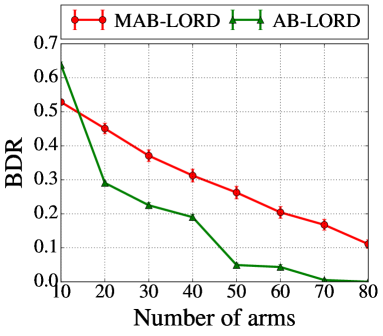
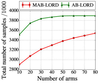
(a)	(b)

Figure 5: (a) BDR over number of arms, i.e. truncation time per hypothesis for $10$ arms and (b) Sample complexity over number of arms for truncation time $M=130000$ for Bernoulli draws, $30$ hypotheses with $12$ non-nulls and averaged over $100$ runs.

4.2 mFDR and FDR control

In this section we use simulations to demonstrate the second part of our meta algorithm which deals with the control of the false discovery rate or its modified version. Since bandit algorithms have a very high best-arm discovery guarantee which in practice even exceeds its theoretical guarantee of at least $1-\alpha_{j}$, mFDR and FDR plots on MAB-FDR  directly do not lead to very insightful plots - namely the constant $0$ line. However, we can demonstrate that even under adversarial conditions, i.e. when the $P$-value under the null is much less concentrated around one than obtained via the best arm bandit algorithm, mFDR or the false discovery proportion (FDP) in each run are still controlled at any time $t$ as Theorem 1 guarantees. Albeit not exactly reflecting mFDR control in the case of MAB-FDR  but in fact in an even harder setting, results from these experiments can be regarded as valuable on their own - it emphasizes the fact that Theorem 1 guarantees mFDR control independent of the adaptive sampling algorithm and specific choice of $p$-value as long as it is always valid.

For Figure 6, we again consider Gaussian draws with the same settings as described in 4.1. This time however, for each true null hypothesis we skip the bandit experiment and directly draw $P^{j}\sim[0,1]$ to compare with the significance levels $\alpha_{j}$ from our online FDR procedure 2. As mentioned above, by Theorem 1, mFDR should still be controlled as it only requires the $p$-values to be super-uniform. In Figure 6(a) we plot the instantaneous false discovery proportion (number of false discoveries over total discoveries) $\text{FDP}(J)=\frac{\sum_{j\in\mathcal{H}_{0}{J}}R_{j}}{\sum_{j=1}^{T}R_{j}}$ over the hypothesis index for different runs with the same settings. Apart from fluctuations in the beginning due to the relatively small denominator, we can observe how the guarantee for the $\text{FDR}(J)=\mathbb{E}\>\>\text{FDP}(J)$, with its empirical value depicted by the red line, transfers to the control of each individual run (blue lines).

In Figure 6, we compare the mFDR (which in fact coincides with the FDR in this plot) of MAB-FDR using different multiple testing procedures, including MAB-IND and a Bonferroni type correction. The latter uses a simple union bound and chooses $\alpha_{j}$ such that $\sum_{j=1}^{\infty}\alpha_{j}\leq\alpha$ and thus trivially allows for any time FWER, and thus FDR control. In our simulations we use $\alpha_{j}=\frac{6\alpha}{\pi^{2}j^{2}}$. As expected, Bonferroni is too conservative and barely makes any rejections whereas the naive MAB-IND approach does not control FDR. LORD avoids both extremes and controls FDR while having reasonable power.

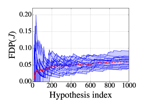
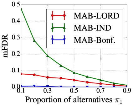
(a)	(b)

Figure 6: (a) Single runs of MAB-LORD (blue) and their average (red) with uniformly drawn $p$-values for null hypotheses and Gaussian draws for non-nulls with $\mu_{i_{\star}}=8$, $\Delta=3$ and $T_{S}=200$, $500$ hypotheses with $200$ true nulls and $30$ arms, the desired mFDR level is $\alpha=0.1$ (b) mFDR over different proportions of non-nulls $\pi_{1}$, with same settings, averaged over $80$ runs.

5 Proofs

In this section we provide the proofs of the main results in the paper.

5.1 Proof of Proposition 1

For any fixed $\gamma\in(0,1)$, we have the equivalence

$$\widehat{\mu}_{i,n_{i}(t)}-\varphi_{n_{i}(t)}(\tfrac{\gamma}{2K})>\widehat{\mu}_{0,n_{0}(t)}+\varphi_{n_{0}(t)}(\tfrac{\gamma}{2})+\epsilon\quad\Longleftrightarrow\quad p_{i,t}\leq\gamma.$$

If $\max\limits_{i=1,\dots,K}\mu_{i}\leq\mu_{0}+\epsilon$, then we have

$$\mathbb{P}\left(\bigcup_{i=1}^{K}\bigcup_{t=1}^{\infty}\Big{\{}\widehat{\mu}_{i,n_{i}(t)}-\varphi_{n_{i}(t)}(\tfrac{\gamma}{2K})>\widehat{\mu}_{0,n_{0}(t)}+\varphi_{n_{0}(t)}(\tfrac{\gamma}{2})+\epsilon\Big{\}}\right)$$

$$=1-\mathbb{P}\left(\bigcap_{i=1}^{K}\bigcap_{t=1}^{\infty}\Big{\{}\widehat{\mu}_{i,n_{i}(t)}-\varphi_{n_{i}(t)}(\tfrac{\gamma}{2K})\leq\widehat{\mu}_{0,n_{0}(t)}+\varphi_{n_{0}(t)}(\tfrac{\gamma}{2})+\epsilon\Big{\}}\right)$$

$$\leq 1-\mathbb{P}\left(\bigcap_{t=1}^{\infty}\Big{\{}\mu_{0}\leq\widehat{\mu}_{0,t}+\varphi_{t}(\tfrac{\gamma}{2})\Big{\}}\cap\bigcap_{i=1}^{K}\bigcap_{t=1}^{\infty}\Big{\{}\widehat{\mu}_{i,n_{i}(t)}-\varphi_{n_{i}(t)}(\tfrac{\gamma}{2K})\leq\mu_{i}\Big{\}}\right)$$

$$\leq\mathbb{P}\left(\bigcup_{t=1}^{\infty}\Big{\{}\mu_{0}>\widehat{\mu}_{0,t}+\varphi_{t}(\tfrac{\gamma}{2})\Big{\}}\right)+\sum_{i=1}^{K}\mathbb{P}\left(\bigcup_{t=1}^{\infty}\Big{\{}\widehat{\mu}_{i,n_{i}(t)}-\varphi_{n_{i}(t)}(\tfrac{\gamma}{2K})>\mu_{i}\Big{\}}\right)$$

$$\leq\tfrac{\gamma}{2}+K\tfrac{\gamma}{2K}=\gamma$$

by equation (4). Thus, we have $\mathbb{P}\left(\bigcup_{i=1}^{K}\bigcup_{t=1}^{\infty}\Big{\{}p_{i,t}\leq\gamma\Big{\}}\right)\leq\gamma$, which completes the proof.

5.2 Proof of Proposition 2

Here we prove that the algorithm 1 terminates in finite time. The technical proof for sample complexity is moved to the Appendix C. It suffices to argue for $\delta/2\leq 0.1$ and we discuss the other case at the end.

Proof of termination in finite time

First we prove by contradiction that the algorithm terminates in finite time with probability one for the case $\mu_{0}\geq\max_{i=1,\dots,K}\mu_{i}-\epsilon$.

Assuming that there exist runs for which the algorithm does not terminate, the set of arms defined by

$$S:=\{i:\text{LCB}_{0}(t)\leq\text{UCB}_{i}(t)-\epsilon\text{ infinitely often (i.o.)}\}$$

is necessarily non-empty for these runs. We now show that this assumption yields a contradiction so that

$$\mathbb{P}(\text{Algorithm does not terminate})\leq\mathbb{P}(\text{LCB}_{0}(t)\leq\max_{i=1,\dots,K}\text{UCB}_{i}(t)-\epsilon\text{ i.o.})=0$$ (11)

First take note that by definition of the algorithm, if an arm $i$ is drawn infinitely often (i.o.), then so is the control arm $0$ and we have $\text{LCB}_{0}(t)\to\mu_{0}$ as well as $\text{UCB}_{i}(t)\to\mu_{i}$ as $t\to\infty$. This follows by the law of large numbers combined with the fact that $\varphi_{n_{i}(t)},\varphi_{n_{0}(t)}\to 0$ as $t\to\infty$, since $\varphi_{n}\to 0$ as $n\to\infty$. Since for the null hypothesis we have $\mu_{0}>\mu_{i}-\epsilon$, it follows that $\text{LCB}_{0}(t)>\text{UCB}_{i}(t)-\epsilon$ for all $t\geq t^{\prime}$ for some $t^{\prime}$.

This argument implies that all arms $i\in S$ can only be drawn a finite number of times, i.e. $n_{i}(t)<\infty$ for all $i\in S$. However, the fact that they are not drawn i.o. implies that $h_{t}\neq i$ and $\ell_{t}\neq i$ i.o. for all $i\in S$, so that there exists $i^{\prime}\not\in S$ such that $\max_{i\in S}\text{UCB}_{i}(t)\leq\text{UCB}_{i^{\prime}}(t)$ i.o. By definition of $S$ we then obtain

$$\text{LCB}_{0}(t)\leq\text{UCB}_{i^{\prime}}(t)-\epsilon\text{ i.o. }$$ (12)

However, since $i^{\prime}\not\in S$, inequality (12) cannot hold and equation (11) is proved.

A nearly identical argument to the above shows that the stopping condition is met in finite time.

5.3 Proof of Theorem 1

We now turn to the proof of Theorem 1, splitting our argument into parts (a) and (b), respectively.

5.3.1 Proof of part (a)

In order for generalized alpha-investing procedures such as LORD to successfully control the mFDR, it is sufficient that $p$-values under the null be conditionally super-uniform, meaning that for all $j\in\mathcal{H}_{0}$, we have

$$\mathbb{P}_{0}(P^{j}\leq\alpha_{j}|\mathcal{F}^{j-1})\leq\alpha_{j}(R_{1},\dots,R_{j-1})$$ (13)

where $\mathcal{F}^{j-1}$ is the $\sigma$-field induced by $R_{1},\dots,R_{j-1}$. Note that as long as condition (13) is satisfied, $T_{j}$ and thus $P^{j}$ could potentially depend on $\alpha_{j}$, i.e. the rejection indicator variables $R_{1},\dots,R_{j-1}$ and potentially $P^{1},\dots,P^{j-1}$. See Aharoni and Rosset [3] for further details.

It thus suffices to show that condition (13) holds for our definition of $p$-value in our framework. We know that by Proposition 1 we have for any random stopping time, thus any fixed truncation time $M$, that $\mathbb{P}_{0}(P^{j}_{T}\leq\alpha_{j})\leq\alpha_{j}$. We now show that the same bound also holds for the ($\alpha_{j}$-dependent) bandit stopping time $T(\alpha_{j})$, i.e. that $\mathbb{P}_{0}(P^{j}_{T(\alpha_{j})}\leq\alpha_{j})\leq\alpha_{j}$.

Under the null hypothesis, the best arm is at most $\epsilon$ better than the control arm, i.e. $\mu_{0}>\mu_{i}-\epsilon$, so that by Proposition 2 we have that with probability $\geq 1-\alpha_{j}$, $i_{b}=0$, i.e. $\text{LCB}_{0}(t)>\text{UCB}_{i}(t)-\epsilon$ for all $i\neq 0$. Hence, $\text{LCB}_{i}(t)-\text{UCB}_{0}(t)<\epsilon$, and thus, by the definition of the $p$-values, $P^{j}_{i,T(\alpha_{j})}=1$ for all $i$ with probability $\geq 1-\alpha_{j}$. It finally follows that $\mathbb{P}_{0}(P^{j}_{T(\alpha_{j})}\leq\alpha_{j})\leq\alpha_{j}$.

Putting things together, under the true null hypothesis (omitting the index $j\in\mathcal{H}_{0}$ to simplify notation) we directly have that for any $\alpha_{j}$

$$\mathbb{P}_{0}(P^{j}_{T_{j}}(\alpha_{j})\leq\alpha_{j}) =\mathbb{P}_{0}\big{(}P^{j}_{T(\alpha_{j})}\leq\alpha_{j}\big{|}T(\alpha_{j})\leq M\big{)}\mathbb{P}_{0}(T(\alpha_{j})\leq M)$$

$$+\mathbb{P}_{0}\big{(}P^{j}_{M}\leq\alpha_{j}\big{|}T(\alpha_{j})>M\big{)}\mathbb{P}_{0}(T(\alpha_{j})>M)$$

$$\leq\alpha_{j}(\mathbb{P}_{0}(T(\alpha_{j})\leq M)+\mathbb{P}_{0}(T(\alpha_{j})>M))=\alpha_{j}$$

for all fixed $\alpha_{j}$ even when the stopping time $T(\alpha_{j})$ is dependent on $\alpha_{j}$. This is equivalent to stating that for any sequence $R_{1},\dots,R_{j-1}$ we have

$$\mathbb{P}_{0}(P^{j}\leq\alpha_{j}(R_{1},\dots,R_{j-1})|\mathcal{F}^{j-1}) =\mathbb{P}_{0}(P^{j}_{T(\alpha_{j}(R_{1},\dots,R_{j-1}))}\leq\alpha_{j}(R_{1},\dots,R_{j-1}))$$

$$\leq\alpha_{j}(R_{1},\dots,R_{j-1})$$

and the proof is complete.

5.3.2 Proof of part (b)

It suffices to prove that for a single experiment $j$ and $M=\infty$, we have $\mathbb{P}_{1}(P^{j}_{T(\alpha_{j})}\leq\alpha_{j})\geq 1-\alpha_{j}$ where $\mathbb{P}_{1}$ is the distribution of a non-null experiment $j$. First observe that at stopping time $T(\alpha_{j})$ of Algorithm 1, either $P^{j}_{i,T(\alpha_{j})}\leq\alpha_{j}$ or $P^{j}_{i,T(\alpha_{j})}=1$ for all $i$. The former event happens whenever the algorithm exits with $i_{b}\in\mathcal{S}^{\star}$, i.e. when $\text{LCB}_{i_{b}}(t)\geq\text{UCB}_{\ell_{t}}(t)-\epsilon$ holds. Then, by definition of the $p$-value in equation (6) and $\ell_{t}$ we must have that $P^{j}_{i_{b},T(\alpha_{j})}\leq\alpha_{j}$. As a consequence, by Proposition 2, we have

$$\mathbb{P}_{1}(P^{j}_{T(\alpha_{j})}\leq\alpha_{j}) \geq\mathbb{P}(P^{j}_{T(\alpha_{j})}\leq\alpha_{j})$$

$$\geq\mathbb{P}_{1}(\text{Algorithm~{}\ref{AlgoModLUCB} exits with}\>i_{b}\in\mathcal{S}^{\star})$$

$$\geq 1-\alpha_{j}$$

and the proof is complete.

6 Discussion

The recent focus in popular media about the lack of reproducibility of scientific results erodes the public’s confidence in published scientific research. To maintain high standards of published results and claimed discoveries, simply increasing the statistical significance standards of each individual experimental work (e.g., reject at level 0.001 rather than 0.05) would drastically hurt power. We take the alternative approach of controlling the ratio of false discoveries to claimed discoveries at some desired value (e.g., 0.05) over many sequential experiments. This means that the statistical significance for validating a discovery changes from experiment to experiment, and could be larger or smaller than 0.05, requiring less or more data to be collected. Unlike earlier works on online FDR control, our framework synchronously interacts with adaptive sampling methods like MABs over uniform sampling to make the overall sampling procedure as efficient as possible. We do not know of other works in the literature combining the benefits of adaptive sampling and FDR control. It should be clear that any improvement, theoretical or practical, to either online FDR algorithms or best-arm identification in MAB (or their variants), immediately results in a corresponding improvement for our MAB-FDR framework.

More general notions of FDR with corresponding online procedures have recently been developed by Ramdas et al [14]. In particular, they incorporate the notion of memory and a priori importance of each hypothesis. This could prove to be a valuable extension for our setting, especially in cases when only the percentage of wrong rejections in the recent past matters. It would be useful to establish FDR control for these generalized notions of FDR as well.

There are several directions that could be explored in future work. First, it would be interesting to extend the MAB aspect (in which each arm is univariate) of our framework to more general settings. Balasubramani and Ramdas [7] show how to construct sequential tests for many multivariate nonparametric testing problems, using LIL confidence intervals, which can again be inverted to provide always valid p-values. It might be of interest to marry the ideas in our paper with theirs. For example, the null hypothesis might be that the control arm has the same (multivariate) mean as other arms ($K$-sample testing), and under the alternative, we would like to pick the arm whose mean is furthest away from the control. A more complicated example could involve dependence, where we observe pairs of arms, and the null hypothesis is that the rewards in the control arm are independent of the alternatives, and if the null is false we may want to pick the most correlated arm. The work by Zhao et al. [15] on tightening LIL-bounds could be practically relevant. Recent work on sequential p-values by Malek et al. [16] also naturally fit into our framework. Lastly, in this work we treat samples or pulls from arms as identical from a statistical perspective; it might be of interest in subsequent work to extend our framework to the contextual bandit setting, in which the samples are associated with features to aid exploration.

Acknowledgements

This work was partially supported by Office of Naval Research MURI grant DOD-002888, Air Force Office of Scientific Research Grant AFOSR-FA9550-14-1-001, and National Science Foundation Grants CIF-31712-23800 and DMS-1309356.

Appendix A Notation

Notation	Terminology and explanation
MAB	(pure exploration for best-arm identification in) multi-armed bandits
$\text{FDR}(J)$	the expected ratio of # false discoveries to # discoveries up to experiment $J$
$\text{mFDR}(J)$	the ratio of expected # false discoveries to expected # discoveries
$\alpha$	target for FDR or mFDR control after any number of experiments
$\text{BDR}(J)$	the best arm discovery rate (generalization of test power)
$\epsilon\text{BDR}(J)$	the $\epsilon$-best arm discovery rate (softer metric than BDR)
$\text{LCB},\text{UCB}$	the lower and upper confidence bounds used in the best-arm algorithms
$j\in\mathbb{N}$	experiment counter (number of MAB instances)
$T_{j}\in\mathbb{N}$	stopping time for the $j$-th experiment
$P^{j}_{t},P_{t}\in[0,1]$	always valid $p$-value after time $t$ (in experiment $j$, explicit or implicit)
$P^{j}$	always valid $p$-value for experiment $j$ at its stopping time $T_{j}$
$\alpha_{j}\in[0,1]$	threshold set by the online FDR algorithm for $P^{j}$, using $\{p_{i}\}_{i=1}^{j-1}$
$T(\alpha_{j})\in\mathbb{N}$	stopping time for the $j$-th experiment, when experiment uses $\alpha_{j}$
0	the control or default arm
$\{1,\dots,K\}$	$K=K(j)$ alternatives or treatment arms (experiment $j$ implicit)
$i\in\{0,\ldots,K\}$	$K+1$ options or “all arms”
$i_{\star},i_{b}$	the best of all arms, and the arm returned by MAB
$\mu_{i},\mu_{*}$	the mean of the $i$-th arm, and the mean of the best arm
$t,n_{i}(t)\in\mathbb{N}$	total number of pulls, number of times arm $i$ is pulled up to time $t$

Table 1: Common notation used throughout the paper.

Appendix B Notes on FDR control

We can prove FDR control for our framework using the specific online FDR procedure called LORD ’15 introduced in [13]. When used in Procedure 2, the only adjustment that needs to be made is to reset $W(j+1)$ to $\alpha$ in step 2 after every rejection, yielding $\alpha_{j}=\alpha\gamma_{j-\tau_{j}}$ for any sequence $\{\gamma_{j}\}_{j=1}^{\infty}$ such that $\sum_{j=1}^{\infty}\gamma_{j}=1$. We call the adjusted procedure MAB-LORD’ for short.

Theorem 2 (Online FDR control for MAB-LORD).

1. MAB-LORD’ achieves mFDR and FDR control at a specified level $\alpha$ for stopping times $T_{j}=\min\{T(\alpha_{j}),M\}$.

2. Furthermore, if we set $M=\infty$, MAB-LORD’ satisfies

   $$\epsilon\text{BDR}(J)\geq\frac{(1-\alpha)}{|\mathcal{H}_{1}(J)|}.$$ (14)

Note that LORD as in [13] is less powerful than in [4] since the values $\alpha_{j}$ in the former can be much smaller than those in [4], which could in fact exceed the level $\alpha$. Therefore, for FDR control we currently do have to sacrifice some power.

Proof.

We leverage the proposition that can be obtained from a slightly more careful analysis of the procedure than in [13].

Proposition 3.

If $\mathbb{P}_{0}(P^{j}\leq\alpha_{j}\mid\tau_{j})\leq\alpha_{j}$, i.e. the distribution of the $p-$values under the null are superuniform conditioned on the last rejection, using the online LORD’15 procedure controls the FDR at each $t$.

Note that this proposition allows online FDR control for any, possibly dependent, $p$-values which are conditionally superuniform. This condition is not equivalent to (13) in general, it is in fact less restrictive since the probability is conditioned only on a function $\widetilde{\tau}_{j}=\max\{k\leq j:R_{k}=1\}$ of all past rejections. Formally, the sigma algebra induced by $\tau_{j-1}$ is contained in $\mathcal{F}^{j-1}$ and hence $\mathbb{P}_{0}(P^{j}\leq\alpha_{j}\mid\tau_{j-1})\leq\mathbb{P}_{0}(P^{j}\leq\alpha_{j}\mid R_{1},\dots,R_{j})$ by the tower property. Finally, utilizing the fact that our $p$-values are conditionally super-uniform as proven in Section 5.3.1, i.e. inequality (13) holds, the condition for Proposition 3 is fulfilled and the proof is complete. ∎

B.1 Proof of Proposition 3

Let $\widetilde{\tau}_{i}$ denote the time of the $i$-th rejection with $\widetilde{\tau}_{0}=0$ (note that this is different from $\tau_{j}$). and define $k(t)=\sum_{j=1}^{t}R_{j}$. Let $H_{j}$ be the $j-$th hypothesis that was rejected. We adjust an argument from [13].

First observe that $\{k(t)=\ell\}=\{\widetilde{\tau}_{\ell}\leq t,\widetilde{\tau}_{\ell+1}>t\}$ and $FDP(t)=FDP(\widetilde{\tau}_{k(t)})$ so that

$$\mathbb{E}FDP(t) =\mathbb{E}FDP(\tau_{k(t)})=\sum_{\ell=1}^{t}\mathbb{E}\big{[}\frac{\sum_{j\in\mathcal{H}_{0}}R_{j}}{\ell}\mid k(t)=\ell\big{]}P(k(t)=\ell)$$

$$=\sum_{\ell=1}^{t}P(k(t)=\ell)\sum_{i=1}^{\ell}\mathbb{E}\big{[}\frac{\mathbbm{1}_{H_{i}\in\mathcal{H}_{0}}}{\ell}\mid k(t)=\ell\big{]}$$

$$=\sum_{\ell=1}^{t}P(k(t)=\ell)\sum_{i=1}^{\ell}\mathbb{E}\big{[}\mathbb{E}\big{(}\frac{\sum_{j=\widetilde{\tau}_{i-1}+1}^{\widetilde{\tau}_{i}}R_{j}\mathbbm{1}_{j\in\mathcal{H}_{0}}}{\ell}\mid\widetilde{\tau}_{0},\dots,\widetilde{\tau}_{i-1}\big{)}\mid\widetilde{\tau}_{\ell}\leq t,\widetilde{\tau}_{\ell+1}>t\big{]}$$

Since for the LORD ’15 procedure, we have $\alpha_{t}=\gamma_{t-\tau_{t}}$, and thus for all positive integers $i$, the random variables $R_{j}$ with $j\geq\widetilde{\tau}_{i-1}$ are conditionally independent of $\widetilde{\tau}_{0},\dots,\widetilde{\tau}_{i-2}$ given $\widetilde{\tau}_{i-1}$. Additionally noting that $\widetilde{\tau}_{i-1}=\tau_{j}$ for all $j\geq\widetilde{\tau}_{i-1}$ by definition of $\widetilde{\tau}$ and $\tau$, using $\mathbb{E}_{0}(\mathbbm{1}_{p_{j}\leq\alpha_{j}}\mid\tau_{j})\leq\alpha_{j}$ we obtain

$$\mathbb{E}\big{(}\frac{\sum_{j\in(\widetilde{\tau}_{i-1},\widetilde{\tau}_{i}]\bigcap j\in\mathcal{H}_{0}}R_{j}}{\ell}\mid\widetilde{\tau}_{0},\dots,\widetilde{\tau}_{i-1}\big{)} =\mathbb{E}\big{(}\frac{\sum_{j=\widetilde{\tau}_{i-1}+1}^{\widetilde{\tau}_{i}}R_{j}\mathbbm{1}_{j\in\mathcal{H}_{0}}}{\ell}\mid\widetilde{\tau}_{i-1}\big{)}$$

$$\leq\frac{\sum_{j=\tau_{i-1}+1}^{\tau_{i}}\mathbbm{1}_{j\in H_{0}}\mathbb{E}[R_{j}\mid\tau_{j}]}{\ell}$$

$$\leq\frac{\sum_{j=\tau_{i-1}+1}^{\tau_{i}}\alpha_{j}}{\ell}\leq\frac{\alpha}{\ell}.$$

The last inequality follows since between any two rejection times $\tau_{k},\tau_{k+1}$, we have

$$\sum_{i=\tau_{k}}^{\tau_{k+1}}\alpha_{i}\leq\alpha\sum_{i=1}^{\infty}\gamma_{i}\leq\alpha.$$

Since $\sum_{\ell=1}^{t}P(k(t)=\ell)=1$ it follows that FDR control is obtained.

Appendix C Proof of sample complexity for Proposition 2

In the sequel we use $\gtrsim,\sim$ for inequality and equality up to constant factors.

Define $i_{\star}=\arg\max_{i=0,1,\dots,K}\mu_{i}$ (breaking ties arbitrarily) and $n_{i}(t)$ to be the number of times sample $i$ was drawn until time $t$. For any $i\in\{0,1,\dots,K\}$ and $\eta\in\mathbb{R}$ we define the following key quantity

$$\tau_{i}(\eta,\xi) :=\min\{n\in\mathbb{N}:2\varphi_{n}(\tfrac{\delta}{2K})<\max\{|\eta-\mu_{i}|,\xi\}\}$$ (15)

$$\lesssim\min\left\{(\eta-\mu_{i})^{-2}\log(K\log(\eta-\mu_{i})^{-2})/\delta),\xi^{-2}\log(K\log(\xi^{-2})/\delta)\right\}$$

where we set $\tau_{i}(\mu_{i},0)=\infty$, but this case does not arise in our analysis.

Let us define the events

$$\mathcal{E}_{i}=\bigcap_{n=1}^{\infty}\{|\widehat{\mu}_{i,n}-\mu_{i}|\leq\varphi_{n}(\tfrac{\delta}{2K})\}.$$

By a union bound and the LIL bound in (4), we have for $\delta/2K<0.1$ that $\mathbb{P}\left(\bigcup_{i=0}^{K}\mathcal{E}_{i}^{c}\right)\leq\frac{K+1}{2K}\delta\leq\delta$ for $K\geq 2$. For $\tfrac{\delta}{2K}>0.1$, note that for all $\delta^{\prime}<\delta$ we have $\varphi_{n}(\delta^{\prime})\leq\varphi_{n}(\delta)$ so that

$$\mathbb{P}(\mathcal{E}_{i}^{c}) =\mathbb{P}(\varphi_{n}(\tfrac{\delta}{2K})<\widehat{\mu}_{i,n}-\mu_{i})$$

$$\leq\mathbb{P}(\varphi_{n}(0.1)<\widehat{\mu}_{i,n}-\mu_{i})\leq\tfrac{\delta}{2K}\qquad\forall i=1,\dots,K$$

Throughout the rest of the proof we assume the events $\mathcal{E}_{i}$ hold.

The following simple lemma regarding the key quantity $\tau_{i}$ will be used throughout the proof.

Lemma 1.

Fix $i\in\{0,1,\dots,K\}$ and $\eta>0$. For any $t\in\mathbb{N}$, whenever $n_{i}(t)\geq\tau_{i}(\eta,\xi)$ we have that under the event $\bigcap_{i=0,\dots,K}\mathcal{E}_{i}$, we have

$$\text{UCB}_{i}(t)\leq\max\{\eta,\mu_{i}+\xi\}\text{ if }\eta\geq\mu_{i}$$

$$\text{LCB}_{i}(t)\geq\min\{\eta,\mu_{i}-\xi\}\text{ if }\eta\leq\mu_{i}$$

Proof.

Assume $n_{i}(t)\geq\tau_{i}(\eta,\xi)$. If $\eta\geq\mu_{i}$ we have by definition of $\mathcal{E}_{i}$ that

$$\text{UCB}_{i}(t)=\widehat{\mu}_{i,n_{i}(t)}+\varphi_{n_{i}(t)}(\tfrac{\delta}{2}) \leq\mu_{i}+2\varphi_{n_{i}(t)}(\tfrac{\delta}{2K})<\mu_{i}+\max\{\eta-\mu_{i},\xi\}$$

and if $\eta\leq\mu_{i}$

$$\text{LCB}_{i}(t)=\widehat{\mu}_{i,n_{i}(t)}-\varphi_{n_{i}(t)}(\tfrac{\delta}{2K}) \geq\mu_{i}-2\varphi_{n_{i}(t)}(\tfrac{\delta}{2K})>\mu_{i}-\max\{\mu_{i}-\eta,\xi\}=\mu_{i}+\min\{\eta-\mu_{i},-\xi\}$$

∎

C.1 Proof of Proposition 2 (a) $\mu_{0}>\max\limits_{i=1,\dots,K}\mu_{i}-\epsilon$

At each time $t$ which does not satisfy the stopping condition, arm $0$ and $\arg\max_{i=1,\dots,K}\text{UCB}_{i}(t)$ are pulled. Note that by Lemma 1

$$\{n_{0}(t)\geq\tau_{0}(\tfrac{\mu_{0}+(\max\limits_{i=1,\dots,K}\mu_{i}-\epsilon)}{2},0)\}\implies\text{LCB}_{0}(t) \geq\min\{\tfrac{\mu_{0}+(\max\limits_{i=1,\dots,K}\mu_{i}-\epsilon)}{2},\mu_{0}\}\geq\tfrac{\mu_{0}+(\max\limits_{i=1,\dots,K}\mu_{i}-\epsilon)}{2}$$ (16)

so that $t>n_{0}(t)$ makes sure that there were enough draws for the particular arm $0$ (since it’s drawn every time). For $i\neq 0$ we have

$$\{n_{i}(t)\geq\tau_{i}(\tfrac{(\mu_{0}+\epsilon)+\max\limits_{i=1,\dots,K}\mu_{i}}{2},0)\}\implies\text{UCB}_{i}(t) \leq\max\{\tfrac{(\mu_{0}+\epsilon)+\max\limits_{i=1,\dots,K}\mu_{i}}{2},\mu_{i}\}\leq\tfrac{(\mu_{0}+\epsilon)+\max\limits_{i=1,\dots,K}\mu_{i}}{2}.$$ (17)

which makes $t>\sum_{i=0}^{K}n_{i}(t)$ a necessary condition.

Reversely whenever $t>\sum_{i=0}^{K}n_{i}(t)$, for all arms $i\neq 0$ we have $\text{UCB}_{i}(t)\leq\tfrac{(\mu_{0}+\epsilon)+\max\limits_{i=1,\dots,K}\mu_{i}}{2}$. In essence, once arm $i$ has been sampled $n_{i}(t)$ times, because of (17), it will not be sampled again - either, because all of the other $UCB_{i}(t)$ satisfy the same upper bound, the algorithm will have stopped, or, if for some $i$ we have $UCB_{i}(t)>\tfrac{(\mu_{0}+\epsilon)+\max\limits_{i=1,\dots,K}\mu_{i}}{2}$ that will be the arm that is drawn. Thus,

$$\{t\geq B_{1}(\mu,\delta):=\tau_{0}(\tfrac{\mu_{0}+(\max\limits_{i=1,\dots,K}\mu_{i}-\epsilon)}{2},0)+\sum_{i=1}^{K}\tau_{i}(\tfrac{(\mu_{0}+\epsilon)+\max\limits_{i=1,\dots,K}\mu_{i}}{2},0)\}$$

$$\implies\{\text{LCB}_{0}(t)-\text{UCB}_{i}(t)\geq-\epsilon\quad\forall i\neq 0\},$$

i.e., the stopping condition is met, where the first term accounts for satisfying (16), the second term accounts for satisfying (17) for all $i\neq 0$, and the third term accounts for satisfying Equation (18). Denoting $T(\delta)$ as the stopping time of the algorithm, this implies that with probability at least $1-\delta$, we have $T(\delta)\leq B_{1}(\mu,\delta)$ and arm $0$ is returned.

Let us now simplify the expression to make it more accessible to the reader and arrive at the theorem statement. Defining $\widetilde{\Delta}_{i}:=\max\{|\eta-\mu_{i}|,\xi\}$ as the effective gap in the definition of $\tau_{i}(\eta,\xi)$ in Equation (15), it is straightforward to verify that the effective gap associated with arm $0$ is equal to

$$\widetilde{\Delta}_{0}\sim(\mu_{0}+\epsilon)-\max\limits_{j=1,\dots,K}\mu_{j},$$

and the effective gap for any other arm $i$ is equal to

$$\widetilde{\Delta}_{i}\gtrsim(\mu_{0}+\epsilon)-\mu_{i}.$$

Using these quantities, we can see that the upper bound $B_{1}(\mu,\delta)$ scales like $\sum_{i=0}^{K}\widetilde{\Delta}_{i}^{-2}\log(K\log(\widetilde{\Delta}_{i}^{-2})/\delta)$.

C.2 Proof of Proposition 2 (b) $\max\limits_{i=1,\dots,K}\mu_{i}=\mu_{i_{\star}}>\mu_{0}+\epsilon$

At each time $t$ which does not satisfy the stopping condition, arm $0$ is pulled. Note again that by Lemma 1

$$\{n_{0}(t)\geq\tau_{0}(\tfrac{(\mu_{i_{\star}}-\epsilon)+\mu_{0}}{2},0)\}\implies\text{UCB}_{0}(t) \leq\max\{\tfrac{(\mu_{i_{\star}}-\epsilon)+\mu_{0}}{2},\mu_{0}\}\leq\frac{(\mu_{i_{\star}}-\epsilon)+\mu_{0}}{2}.$$

The following claim is key to proving this case (where $u\in(0,1)$ be an absolute constant to be defined later).

Claim 1.

Under the event $\bigcap_{i=0,\dots,K}\mathcal{E}_{i}$, for any $u\leq\tfrac{2}{7}$ and $\bar{\mu}\in[\max_{j\neq i_{\star}}\mu_{j},\mu_{i_{\star}}]$, we have

$$|\{s\geq 2\sum_{i=0}^{K}\tau_{i}(\bar{\mu},u\epsilon):\text{LCB}_{h_{s}}(s)\leq\mu_{i_{\star}}-\tfrac{5}{2}u\epsilon\text{ or }\text{UCB}_{\ell_{s}}(s)\geq\mu_{i_{\star}}+u\epsilon\}|<\sum_{i=0}^{K}\tau_{i}(\bar{\mu},u\epsilon)$$ (18)

The proof of this claim can be found in Appendix C.3. Note that for all $s$ we have that

$$\text{LCB}_{h_{s}}(s)\geq\mu_{i_{\star}}-\tfrac{5}{2}u\epsilon\text{ and }\text{UCB}_{\ell_{s}}(s)\leq\mu_{i_{\star}}+u\epsilon\implies\text{LCB}_{h_{s}}(s)\geq\text{UCB}_{\ell_{s}}(s)-\epsilon.$$

Intuitively the inequality (18) thus limits the number of times that for $t\geq 2\sum_{i=0}^{K}\tau_{i}(\bar{\mu},u\epsilon)$, the criterion $\text{LCB}_{h_{s}}(s)\geq\text{UCB}_{\ell_{s}}(s)-\epsilon$ is not fulfilled. We refer to the times when the condition on the left hand side of inequality (18) is fulfilled, as “good” times.

Applying Claim 1 with $\bar{\mu}=\max_{j\neq i_{\star}}\tfrac{\mu_{i_{\star}}+\mu_{j}}{2}$ and $u=\frac{\mu_{i_{\star}}-(\mu_{0}+\epsilon)}{5\epsilon}$ we then observe that on the “good” times, we have

$$\text{LCB}_{h_{t}}\geq\mu_{i_{\star}}-\tfrac{5}{2}u\epsilon=\frac{\mu_{i_{\star}}+(\mu_{0}+\epsilon)}{2}=\frac{(\mu_{i_{\star}}-\epsilon)+\mu_{0}}{2}+\epsilon,$$

so that we directly obtain that with probability at least $1-\delta$,

$$T(\delta)\leq B_{2}(\mu,\delta):=\tau_{0}(\tfrac{(\mu_{i_{\star}}-\epsilon)+\mu_{0}}{2},0)+3\sum_{i=0}^{K}\tau_{i}(\max_{j\neq i_{\star}}\tfrac{\mu_{i_{\star}}+\mu_{j}}{2},\min\{\tfrac{2}{7}\epsilon,\tfrac{\mu_{i_{\star}}-(\mu_{0}+\epsilon)}{5}\}).$$

Let us now simplify the expression. It is straightforward to verify that the effective gap associated with arm $0$ is equal to

$$\widetilde{\Delta}_{0} \gtrsim\min\left\{\tfrac{\mu_{i_{\star}}-(\mu_{0}+\epsilon)}{2},\max\left\{\max_{j\neq i_{\star}}\tfrac{\mu_{i_{\star}}+\mu_{j}}{2}-\mu_{0},\tfrac{2}{7}\epsilon\right\}\right\}$$

$$\gtrsim\min\left\{\mu_{i_{\star}}-(\mu_{0}+\epsilon),\max\{\Delta_{0},\frac{4}{7}\epsilon\}\right\}$$

and the effective gap for any other arm $i$ is equal to

$$\widetilde{\Delta}_{i} =\max\left\{|\max_{j\neq i_{\star}}\tfrac{\mu_{i_{\star}}+\mu_{j}}{2}-\mu_{i}|,\min\{\tfrac{2}{7}\epsilon,\tfrac{\mu_{i_{\star}}-(\mu_{0}+\epsilon)}{5}\}\right\}$$

$$\gtrsim\max\left\{\Delta_{i},\min\left\{\mu_{i_{\star}}-(\mu_{0}+\epsilon),\epsilon\right\}\right\}$$

where we recall that $\Delta_{i}=\mu_{i_{\star}}-\mu_{i}$ if $i\neq i_{\star}$, and $\Delta_{i_{\star}}=\mu_{i_{\star}}-\max_{j\neq i_{\star}}\mu_{j}$ otherwise. Using these quantities, the upper bound $B_{2}(\mu,\delta)$ on the stopping time $T(\delta)$ scales like $\sum_{i=0}^{K}\widetilde{\Delta}_{i}^{-2}\log(K\log(\widetilde{\Delta}_{i}^{-2})/\delta)$. This concludes the proof of the proposition.

C.3 Proof of Claim 1

Let $\bar{\mu}\in[\max_{j\neq i_{\star}}\mu_{j},\mu_{i_{\star}}]$ and $\tau_{i}:=\tau_{i}(\bar{\mu},u\epsilon)$. The following result is a a key ingredient for the proof of the claim.

Proposition 4.

For any time $t$ and $u\leq 1/2$,

$$\Big{\{}|\{s\leq t:h_{s}=i_{\star}\}|\geq\sum_{i=0}^{K}\tau_{i}\Big{\}}$$

$$\implies\{\text{UCB}_{\ell_{t}}(t)\leq\bar{\mu}+u\epsilon\}\cap\{\text{LCB}_{h_{t}}(t)\geq\bar{\mu}-u\epsilon\}$$

$$\implies\{\text{LCB}_{h_{t}}(t)-\text{UCB}_{\ell_{t}}(t)\geq-\epsilon\}.$$

Proof.

If $h_{s}=i_{\star}$ then some $i\neq i_{\star}$ is assigned to $\ell_{s}$ and $\text{UCB}_{i}(s)\leq\max\{\bar{\mu},\mu_{i}+u\epsilon\}\leq\bar{\mu}+u\epsilon$ whenever $n_{i}(s)\geq\tau_{i}(\bar{\mu},u\epsilon)$. Because $\ell_{s}$ is the highest upper confidence bound, the sum over all $\tau_{i}$ represents exhausting all arms (i.e., pigeonhole principle). An analogous result holds for $\text{LCB}_{i_{\star}}(t)$. ∎

A direct consequence of Proposition 4 is that even though we don’t know which arm will be assigned to $h_{t}$ at any given time $t$, we do know that if $h_{t}=i_{\star}$ for a sufficient number of times, namely $\sum_{i=0}^{K}\tau_{i}$ times, the termination criteria will be met. Thus, assume $h_{t}\neq i_{\star}$ and note that

$$\{h_{t}=i,\ \mu_{i}<\mu_{i_{\star}}-\tfrac{5}{2}u\epsilon,\ \widehat{\mu}_{i,n_{i}(t)}\geq\min\{\bar{\mu},\mu_{i_{\star}}-\tfrac{3}{2}u\epsilon\}\}$$

$$\implies\min\{\bar{\mu},\mu_{i_{\star}}-\tfrac{3}{2}u\epsilon\}\leq\widehat{\mu}_{i,n_{i}(t)}\leq\mu_{i}+\varphi_{n_{i}(t)}(\tfrac{\delta}{2K})$$

$$\implies\{n_{i}(t)<\tau_{i}\}$$

where the last line follows from $\mu_{i}+\varphi_{n_{i}(t)}(\tfrac{\delta}{2K})<\min\{\bar{\mu},\mu_{i}+u\epsilon\}\leq\min\{\bar{\mu},\mu_{i_{\star}}-\tfrac{3}{2}u\epsilon\}$ whenever $n_{i}(t)\geq\tau_{i}$. Furthermore, the following Proposition 5, says for $t\geq 2\sum_{i=0}^{K}\tau_{i}$ we have that $\widehat{\mu}_{h_{t},n_{h_{t}}(t)}\geq\min\{\bar{\mu},\mu_{i_{\star}}-\tfrac{3}{2}u\epsilon\}$.

Proposition 5.

For any time $t$,

$$\{t\geq 2\sum_{i=0}^{K}\tau_{i}\}\implies\{\widehat{\mu}_{h_{t},n_{h_{t}}(t)}\geq\min\{\bar{\mu},\mu_{i_{\star}}-\tfrac{3}{2}u\epsilon\}\}.$$

The proof of the proposition can be found in Section C.4.

Combining this fact with the display immediately above and the observation that some $i=h_{t}$, we have that $|\{s\geq 2\sum_{i=0}^{K}\tau_{i}:\mu_{i_{\star}}-\mu_{h_{s}}\geq\tfrac{5}{2}u\epsilon\}|<\sum_{i=0}^{K}\tau_{i}$. Now, on one of these times $t$ such that $\{h_{t}=i,n_{i}(t)\geq\tau_{i},\mu_{i_{\star}}-\mu_{i}<\tfrac{5}{2}u\epsilon\}$, we have

$$\text{LCB}_{i}(t)=\widehat{\mu}_{i,n_{i}(t)}-\varphi_{n_{i}(t)}(\tfrac{\delta}{2K})\geq\mu_{i}-2\varphi_{n_{i}(t)}(\tfrac{\delta}{2K})\geq\min\{\bar{\mu},\mu_{i}-u\epsilon\}\geq\mu_{i_{\star}}-\tfrac{5}{2}u\epsilon.$$

The above display with the next proposition completes the proof of Equation 18.

Proposition 6.

For any time $t$,

$$\{t\geq\sum_{i=0}^{K}\tau_{i}\}\implies\{\max_{i=0,1,\dots,K}\text{UCB}_{i}(t)\leq\mu_{i_{\star}}+u\epsilon\}.$$

Proof.

Note that

$$\{\text{UCB}_{i}(t)\geq\mu_{i_{\star}}+u\epsilon\} \implies\{\mu_{i_{\star}}+u\epsilon\leq\text{UCB}_{i}(t)=\widehat{\mu}_{i,n_{i}(t)}+\varphi_{n_{i}(t)}(\tfrac{\delta}{2})\leq\mu_{i}+2\varphi_{n_{i}(t)}(\tfrac{\delta}{2K})\}$$

$$\implies\{n_{i}(t)<\tau_{i}\}$$

since $\mu_{i}+2\varphi_{n_{i}(t)}(\tfrac{\delta}{2K})<\max\{\bar{\mu},\mu_{i}+u\epsilon\}\leq\mu_{i_{\star}}+u\epsilon$ whenever $n_{i}(t)\geq\tau_{i}$. Now, because at each time $t$, the arm $\arg\max_{j=0,1,\dots,K}\text{UCB}_{j}(t)$ is pulled because it is either $h_{t}$ or $\ell_{t}$, we conclude that this arm can only be pulled $\tau_{i}$ times before satisfying $\text{UCB}_{i}(t)\leq\mu_{i_{\star}}+u\epsilon$. ∎

C.4 Proof of Proposition 5

The above proposition implies,

$$\{t\geq 2\sum_{i=0}^{K}\tau_{i}\}\implies\left\{|\{s\leq t:h_{s}\neq i_{\star}\}|\geq\sum_{i=0}^{K}\tau_{i}\right\}.$$

Now consider the event

$$\{h_{t}\neq i_{\star},\ell_{t}=i\} \implies\mu_{i_{\star}}\leq\widehat{\mu}_{i_{\star},n_{i_{\star}}(t)}+\varphi_{n_{i_{\star}}(t)}(\tfrac{\delta}{2})\leq\widehat{\mu}_{i,n_{i}(t)}+\varphi_{n_{i}(t)}(\tfrac{\delta}{2})\leq\mu_{i}+2\varphi_{n_{i}(t)}(\tfrac{\delta}{2K})$$

$$\implies\{\mu_{i_{\star}}-\mu_{i}\leq 2\varphi_{n_{i}(t)}(\tfrac{\delta}{2K})\}$$

$$\implies\{n_{i}(t)<\tau_{i}\}\cup\{n_{i}(t)\geq\tau_{i},\mu_{i_{\star}}-\mu_{i}\leq 2\varphi_{n_{i}(t)}(\tfrac{\delta}{2K})\}$$

$$\implies\{n_{i}(t)<\tau_{i}\}\cup\{n_{i}(t)\geq\tau_{i},\mu_{i_{\star}}-\mu_{i}\leq\max\{|\bar{\mu}-\mu_{i}|,u\epsilon\}\}$$

$$\implies\{n_{i}(t)<\tau_{i}\}\cup\{n_{i}(t)\geq\tau_{i},\mu_{i_{\star}}-\mu_{i}<u\epsilon\}\cup\{n_{i}(t)\geq\tau_{i},i=i_{\star}\}$$

by the definition of $\tau_{i}$. Because at each time $s\leq t$ we have that some $i=\ell_{s}$, if $|\{s\leq t:h_{s}\neq i_{\star}\}|\geq\sum_{i=0}^{K}\tau_{i}$, we have that

$$\{t\geq 2\sum_{i=0}^{K}\tau_{i}\}\implies\{\exists i:n_{i}(t)\geq\tau_{i}\text{ and }\mu_{i_{\star}}-\mu_{i}<u\epsilon\}\cup\{n_{i}(t)\geq\tau_{i}\text{ and }i=i_{\star}\}.$$

We use the fact that such an $\ell_{t}=i\neq i_{\star}$ exists that satisfies $\mu_{i_{\star}}-\mu_{i}<u\epsilon$ to say

$$\exists i\neq i_{\star}:\widehat{\mu}_{i,n_{i}(t)}\geq\mu_{i}-\varphi_{n_{i}(t)}(\tfrac{\delta}{2K})\geq\mu_{i}-\max\{\mu_{i_{\star}}-\mu_{i},u\epsilon\}/2\geq\mu_{i_{\star}}-\tfrac{3}{2}u\epsilon$$

or $\ell_{t}=i_{\star}$ and

$$\widehat{\mu}_{i_{\star},n_{i_{\star}}(t)}\geq\mu_{i_{\star}}-\varphi_{n_{i_{\star}}(t)}(\tfrac{\delta}{2K})\geq\mu_{i_{\star}}-\max\{\mu_{i_{\star}}-\bar{\mu},u\epsilon\}/2=\min\{\bar{\mu},\mu_{i_{\star}}-\tfrac{1}{2}u\epsilon\}.$$

Because $\widehat{\mu}_{h_{t},n_{h_{t}}(t)}\geq\max_{i=0,1,\dots,K}\widehat{\mu}_{i,n_{i}(t)}$, the proof of the claim is complete.

References

- [1] Y. Benjamini and Y. Hochberg, “Controlling the false discovery rate: a practical and powerful approach to multiple testing,” Journal of the Royal Statistical Society. Series B (Methodological), pp. 289–300, 1995.
- [2] D. P. Foster and R. A. Stine, “-investing: a procedure for sequential control of expected false discoveries,” Journal of the Royal Statistical Society: Series B (Statistical Methodology), vol. 70, no. 2, pp. 429–444, 2008.
- [3] E. Aharoni and S. Rosset, “Generalized -investing: definitions, optimality results and application to public databases,” Journal of the Royal Statistical Society: Series B (Statistical Methodology), vol. 76, no. 4, pp. 771–794, 2014.
- [4] A. Javanmard and A. Montanari, “Online rules for control of false discovery rate and false discovery exceedance,” The Annals of Statistics, 2017.
- [5] R. Johari, L. Pekelis, and D. J. Walsh, “Always valid inference: Bringing sequential analysis to A/B testing,” arXiv preprint arXiv:1512.04922, 2015.
- [6] K. G. Jamieson, M. Malloy, R. D. Nowak, and S. Bubeck, “lil’UCB: An optimal exploration algorithm for multi-armed bandits,” in COLT, vol. 35, 2014, pp. 423–439.
- [7] A. Balsubramani and A. Ramdas, “Sequential nonparametric testing with the law of the iterated logarithm,” in Proceedings of the Thirty-Second Conference on Uncertainty in Artificial Intelligence. AUAI Press, 2016, pp. 42–51.
- [8] E. Kaufmann, O. Cappé, and A. Garivier, “On the complexity of best arm identification in multi-armed bandit models,” The Journal of Machine Learning Research, 2015.
- [9] K. Jamieson and R. Nowak, “Best-arm identification algorithms for multi-armed bandits in the fixed confidence setting,” in Information Sciences and Systems (CISS), 2014 48th Annual Conference on. IEEE, 2014, pp. 1–6.
- [10] S. S. Villar, J. Bowden, and J. Wason, “Multi-armed bandit models for the optimal design of clinical trials: benefits and challenges,” Statistical science: a review journal of the Institute of Mathematical Statistics, vol. 30, no. 2, p. 199, 2015.
- [11] S. Kalyanakrishnan, A. Tewari, P. Auer, and P. Stone, “Pac subset selection in stochastic multi-armed bandits,” in Proceedings of the 29th International Conference on Machine Learning (ICML-12), 2012, pp. 655–662.
- [12] M. Simchowitz, K. Jamieson, and B. Recht, “The simulator: Understanding adaptive sampling in the moderate-confidence regime,” arXiv preprint arXiv:1702.05186, 2017.
- [13] A. Javanmard and A. Montanari, “On online control of false discovery rate,” arXiv preprint arXiv:1502.06197, 2015.
- [14] A. Ramdas, F. Yang, M. J. Wainwright, and M. I. Jordan, “Online control of the false discovery rate with decaying memory,” in Advances in Neural Information Processing Systems (NIPS) 2017, arXiv preprint arXiv:1710.00499, 2017.
- [15] S. Zhao, E. Zhou, A. Sabharwal, and S. Ermon, “Adaptive concentration inequalities for sequential decision problems,” in Advances In Neural Information Processing Systems, 2016, pp. 1343–1351.
- [16] A. Malek, Y. Chow, M. Ghavamzadeh, and S. Katariya, “Sequential multiple hypothesis testing with type I error control,” in The 20th International Conference on Artificial Intelligence and Statistics, 2017, 2017, pp. 1343–1351.