A Practical Algorithm for Enumerating Collinear Points

Abstract.

This paper studies the problem of enumerating all maximal collinear subsets of size at least three in a given set of $n$ points. An algorithm for this problem, besides solving degeneracy testing and the exact fitting problem, can also help with other problems, such as point line cover and general position subset selection. The classic topological sweeping algorithm of Edelsbrunner and Guibas can find these subsets in $O(n^{2})$ time in the dual plane. We present an alternative algorithm that, although asymptotically slower than their algorithm in the worst case, is simpler to implement and more amenable to parallelization. If the input points are decomposed into $m$ convex polygons, our algorithm has time complexity $O(n^{2}\log m)$ and space complexity $O(n)$. Our algorithm can be parallelized on the CREW PRAM with time complexity $O(n\log m)$ using $n$ processors.

1. Introduction

We study the problem of finding all maximal collinear subsets of size at least three in a given set of points in the plane. In this paper, we assume the real RAM model of computation, where real arithmetic operations and comparison of reals take constant time and the floor function ($\lfloor a\rfloor$) is not allowed [1].

Our main motivation is that some of the algorithms for problems like point line cover (i.e., covering a set of points with the minimum number of lines) [2] or general position subset selection (finding the largest subset of points in general position) [3] need to identify maximal collinear subsets as a first step. A special case of this problem is the well-known degeneracy testing problem (i.e. testing whether any three of the points are collinear). The fastest known algorithm for this problem has time complexity $O(n^{2})$ [4], which seems best possible, based on either the number of sidedness queries [5] or 3-SUM reduction [6]. Another special case is the exact fitting problem, which tries to find the line that covers the most points [7]. Finding maximal collinear subsets trivially solves these two problems.

As with degeneracy testing, the best known algorithm for finding collinear subsets uses topological sweeping with time complexity $O(n^{2})$ and space complexity $O(n)$.

In this paper, we present an alternative algorithm based on cyclically sorting the input points. The algorithm runs in time $O(n^{2}\log m)$ and space $O(n)$, if the input points can be decomposed into $m$ convex polygons. Our algorithm is much easier to implement than those depending on arrangements, and should be almost as fast in practice. The techniques we use for sorting the points cyclically may be helpful in other algorithms, such as those for computing visibility graphs. Another advantage of our algorithm is that it can be executed in parallel on the CREW PRAM in time $O(n\log m)$ and space $O(nm)$ using $n$ processors.

The rest of this paper is organized as follows. We summarize related work in Section 2 and present the basis of our algorithm in Section 3 with time complexity $O(n^{2}\log n)$. In Section 4, we improve its time complexity to $O(n^{2}\log m)$, if input points are decomposed into $m$ convex polygons. We present our parallel algorithm in Section 5 and end with some concluding remarks in Section 6.

2. Related Work

The problem of finding collinear subsets can be restated in the dual plane. Each point in the input is mapped to a line in the dual plane. A subset of these lines intersect each other at a common point, if their corresponding points in the original plane are collinear. Therefore, the problem of finding maximal sets of collinear points is equivalent to finding the set of lines that intersect each other at each intersection in the dual plane. Intersecting lines can be identified using plane sweeping with time complexity $O(n^{2}\log n)$ [8]. An alternative for identifying intersecting lines is using an arrangement of lines, i.e. a partition of the plane induced by the set of lines into vertices, edges, and faces. An arrangement has space complexity $O(n^{2})$ and can be constructed with time complexity $O(n^{2})$ [9].

The well-known topological sweeping algorithm of Edelsbrunner and Guibas [4] can sweep arrangements without constructing them, thus reducing its space complexity to $O(n)$. The time complexity matches the lower-bound for the time complexity of the problem of testing degeneracy and is thus the best possible. The algorithm, however, is rather difficult to implement, especially since input points are not in general position (see for instance [10]). Note that reporting line intersections in the dual plane is not enough for finding collinear points. These intersections should also be ordered so that all lines that intersect can be reported at once efficiently, making intersection reporting algorithms (for instance [11]) inefficient for this problem.

Because topological sweeping is inherently sequential and thus unsuitable for parallel execution, parallel algorithms for sweeping or constructing arrangements have appeared in the literature. Anderson et al. [12] presented a CREW PRAM algorithm for constructing arrangements in $O(n\log^{\ast}n)$ time with $O(n)$ processors and Goodrich [13] presented an algorithm (also on the CREW PRAM) with the same goal with time complexity $O(n\log n)$ with $O(n)$ processors. Since these algorithms construct the arrangement, they have space complexity $O(n^{2})$, which is more than the $O(nm)$ space complexity of our parallel algorithm. Our algorithm also beats Goodrich’s in time complexity, besides being easier to code since it uses only simple data structures.

Other methods have been presented to partition the arrangement into smaller regions with fewer points and use the sequential algorithm for sweeping these regions in parallel (e.g. [14] and [15]). They are usually based on the assumption that the points are in general position. Such partitions yield poor performance, when this assumption is violated as it is the case in the problem of finding collinear points. Similar parallel sweeping methods have been presented for specific applications (e.g., rectangle intersection [16] and hidden surface elimination [17]), in which there are fewer events than the number of intersections in the worst case (for finding collinear subsets $\Theta(n^{2})$). More recently, McKenny et al. presented a plane sweep algorithm that divides the plane into vertical slabs perpendicular to the sweep line, which has time complexity $O(n\log n)$ with $n$ processors for $\Theta(n^{2})$ intersections [18], whose cost is more than our algorithm.

3. The Base Algorithm

In what follows, we describe our main algorithm for enumerating maximal collinear subsets of a set of points. It assumes an arbitrary ordering $\sigma$ on the input points $P$. It processes each point $p$ (in the order specified by $\sigma$) and finds and reports all maximal sets of points collinear with $p$ that have not already been found in a previous iteration.

1

2foreach $p$ in $\sigma$ do

3       Sort all points cyclically around $p$ in counterclockwise direction to obtain the sequence $O_{p}$. In other words, for each point $q$ in $P$, let $a_{p}(q)$ be the counterclockwise angle between the horizontal half-line starting from $p$ rightward and the segment $pq$; $O_{p}$ is the result of sorting $P$ according to $a_{p}$.  

4      Decompose $O_{p}$ into sequences $U$ and $D$ while preserving the order of the points, such that $q\in U$ if $a_{p}(q)<\pi$, and $q\in D$, otherwise. Let $\bar{a}_{p}(q)=a_{p}(q)$ for every point $q\in U$ and $\bar{a}_{p}(q)=a_{p}(q)-\pi$ for every point $q\in D$.  

5      Merge $U$ and $D$ by keeping the points ordered by $\bar{a}_{p}$ to obtain $M_{p}$.  

6      Find maximal consecutive collinear points in $M_{p}$. This requires a linear scan through $M_{p}$.  

7      Report the sets found in step 3.1 that do not contain any point that precedes $p$ in $\sigma$.  

Algorithm 3.1 $\operatornamewithlimits{\textsc{collinearPoints}}(\sigma)$

It is not difficult to see that except for step 3.1 of the algorithm, each step has time complexity $O(n)$. Sorting the points in step 3.1 can be performed in $O(n\log n)$. Note that the points in sequences $U$ and $D$ remain sorted according to both $a_{p}$ and $\bar{a}_{p}$ in step 3.1 and can be merged in $O(n)$. Since these steps are repeated for every point, the total time complexity of the algorithm is $O(n^{2}\log n)$ and its space complexity is $O(n)$. Theorem 3.1 shows its correctness.

Theorem 3.1.

The algorithm reports every maximal set of collinear points exactly once.

Proof.

Let $S$ be a set of maximal collinear points in $P$ and let $p$ be the first point of $S$ in $\sigma$. When $P$ is sorted cyclically around $p$, all points of $S$ appear contiguously either in $U$ or in $D$, and when these sequences are merged, in $M_{p}$. Thus, they are identified in step 3.1 and reported in step 3.1, since $p$ was the first point of $S$ in $\sigma$. For every other point $q$ of $S$, although the points of $S$ follow each other in $M_{q}$, they will not be reported in step 3.1, since $p$ is before $q$ in $\sigma$. Note that the algorithm never outputs non-collinear points, thanks to step 3.1. ∎

In what follows, we try to improve the time complexity of step 3.1 (i.e. sorting the points to obtain $O_{p}$). A simple heuristic, which we shall not pursue here, is to adjust $\sigma$ so that consecutive points are as close as possible, so that fewer alterations are made to $O_{p}$. This would help if in step 3.1, the partially sorted sequence for the previous point is sorted for the current point (some sorting algorithms are much faster for sorting partially-sorted sequences). More formally, let $p$ and $q$ be two consecutive points in $\sigma$. A pair of points, $s$ and $t$, is inverted if $s$ appears before $t$ in $O_{p}$ but after $t$ in $O_{q}$. This can happen only if the line passing through $s$ and $t$ intersects the segment from $p$ to $q$. While moving a point $q^{\prime}$ from $p$ to $q$, it can be shown that each such intersection swaps two adjacent points in $O_{q^{\prime}}$. Thus, the goal is to minimize the number of such intersections or inverted pairs.

In the next section we use another method for the same goal: finding sets of points, whose order does not change substantially in $O_{p}$ for different points $p$ in $P$.

4. Using Convex Polygon Decompositions

We now concentrate on improving the complexity of computing $O_{p}$ for every point $p$ in $P$. For that, we try to identify sets of points in $P$ that appear in the same order in $O_{p}$ for every $p$ in $P$. As we show in Lemma 4.1, convex polygons have this property to a large extent. A tangent $l_{pq}$ from a point $p$ to a convex polygon $P$ is a line that passes through $p$ and another point $q$ of $P$ such that all of $P$ lies to one side of $l_{pq}$; $q$ is called the tangent point from $p$ to polygon $P$. If the tangent passes through more than one point of $P$, the closest to $p$ is considered the tangent point. Tangent points can be identified via a linear scan (or binary search) through the points of $P$.

Lemma 4.1.

For any point $p$ and any convex polygon $P=\left(p_{0},p_{1},...,p_{k-1}\right)$, $P$ can be decomposed into at most two sequences such that the points in any of these sequences are cyclically sorted (either clockwise or counterclockwise) from $p$.

Proof.

If $p$ is inside $P$, every point of $P$ appears in the same order when cyclically ordered from $p$; thus, the whole of $P$ is a sorted sequence. Otherwise, let $p_{i}$ and $p_{j}$ be tangent points from $p$ to polygon $P$. Then, the sequences $\left(p_{i},p_{i+1},...,p_{j-1}\right)$ and $\left(p_{j},p_{j+2},...,p_{i-1}\right)$ are cyclically sorted from $p$ (indices are modulo $k$). ∎

Theorem 4.2.

If the set of points $P$ can be decomposed into $m$ convex polygons, the algorithm introduced in Section 3 for identifying collinear points can be improved to achieve the time complexity of $O(n^{2}\log m)$.

Proof.

We modify step 3.1 of the algorithm for calculating $O_{p}$. Based on Lemma 4.1, we can obtain $k$ sequences ($k\leq 2m$), all of which are sorted cyclically around $p$. This can be done in $O(n)$ (to identify the tangent points of the polygons and to create the new sequences). We have to merge these sorted sequences to obtain $O_{p}$. This can be done in $O(n\log m)$ using a heap priority queue: initially the first points of the sorted sequences are inserted into the heap with time complexity $O(m\log m)$. Then, the point $q$ with the smallest value of $a_{p}(q)$ is extracted from the heap and the point with the next smallest $a_{p}$ in $q$’s sequence is inserted into the heap. This process is repeated $n$ times to obtain $O_{p}$. Since extracting the value from and inserting a new value into the heap can be done in $O(\log m)$, $O_{p}$ can be constructed with time complexity $O(n\log m+m\log m)$, which is equivalent to $O(n\log m)$, since $m<n$. ∎

One method for decomposing a set of points into convex polygons is convex hull peeling, i.e., repeatedly extracting convex hulls from the set (for applications and a survey, the reader may consult [19]). The number of resulting convex hulls is sometimes called convex hull peeling depth. Common convex hull algorithms can be used for convex hull peeling by repeatedly extracting convex hulls in $O(mn\log n)$, if the convex hull peeling depth is $m$ (this seems adequate for our purpose; there are faster algorithms however [20]). This yields the following corollary. Note that most convex hull algorithms can be slightly modified to allow collinear points in the boundary of the hull.

Corollary 4.3.

All maximal collinear subsets of size at least three in a set of $n$ points can be identified in $O(n^{2}\log m)$, where $m$ is the convex hull peeling depth of the points.

Parts (a)–(d) of Figure 1 demonstrate the steps of the algorithm described in this section for decomposing the set of input points into convex polygons (part (b)), splitting each polygon into at most two cyclically sorted sequences (part (c)), and merging these sequences to obtain $O_{q}$ (part (d); the arrows show the order of processing the points in the sequences). The points on each of the lines $L_{1}$, $L_{2}$, and $L_{3}$ should be contiguous in $M_{p}$.

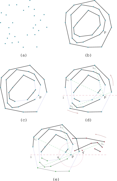
Figure 1. (a)–(b) An input point set $P$ is decomposed into convex layers. The algorithm is currently processing point $p$. (c) The convex layers are decomposed into sorted subsequences, bookended by points tangent to $p$. (d) Subsequences are split up and added to $U$ or $D$ depending on whether they lie above or below the horizontal line $l$ through $p$. (e) Points appearing in $D$ are then mapped to their antipodes and merged with $U$ to obtain $M_{p}$. Collinear points appear contiguous in $M_{p}$.

5. Parallel Algorithm

To obtain a parallel algorithm for finding sets of collinear points, both the algorithm presented in Section 3 and convex polygon decomposition should be performed in parallel, as Theorem 5.2 shows. We shall use the following lemma in the proof of Theorem 5.2.

Lemma 5.1.

If $m<n$, then $m\log n=O(n\log m)$.

Proof.

Suppose for the sake of contradiction that the converse is true, i.e. if $m<n$, then $m\log n>cn\log m$ for some $c\geq 1$ and $n\geq 3$. This implies that $m/\log m>cn/\log n$, a contradiction, since the function $f(x)=x/\log x$ for $x\geq 3$ is monotonically increasing. ∎

We are now ready to prove Theorem 5.2.

Theorem 5.2.

With $O(n)$ processors, it is possible to identify all maximal collinear subsets of a set of $n$ points on the CREW PRAM with time complexity $O(n\log m)$ and space complexity $O(nm)$, where $m$ is the convex hull peeling depth of the points.

Proof.

The parallel algorithm first decomposes the input points into convex polygons and then enumerates collinear subsets of the points. We discuss these two steps separately as follows.

For decomposing points into convex polygons, we use the parallel algorithm presented by Akl [21]: it computes the convex hull of a set of $n$ points in $O(\log n)$ time with $O(n)$ processors. Akl’s algorithm assumes input points to be sorted by their $x$-coordinates; this can be done on the CREW PRAM in $O(\log n)$ with $O(n)$ processors [22]. The convex hull algorithm should be repeated $m$ times, yielding the time complexity of $O(m\log n)$. Thus, the total time complexity of the algorithm is $O(n\log m+m\log n)$, which is equivalent to $O(n\log m)$. This follows trivially if $m=\Theta(n)$. However, if $m=o(n)$ it follows from Lemma 5.1.

Given that there is no dependency between different iterations of the algorithm presented in Section 3, it can be parallelized by distributing the points among the processors, each of which requires $O(n\log m)$ to finish its task with space complexity $O(n)$. Therefore, it remains to improve the overall space complexity of the parallel algorithm to $O(nm)$.

The $O(n)$ space complexity per processor is due to storing the sorted and merged sequences of points ($O_{p}$ and $M_{p}$, as defined in Section 3), storing sequences of points obtained after splitting convex polygons, and storing consecutive collinear points in step 3.1 of the algorithm presented in Section 3. We reduce the space complexity of each processor to $O(m)$ (plus $O(n)$ for storing convex polygons, which is shared among the processors). Instead of storing all elements of a subsequence of a sequence of points, we store two pointers to indicate its start and end positions. Therefore, we can store the subsequences resulting from splitting the polygons in $O(m)$ (there are at most $2m$ such subsequences).

We now modify the base algorithm not to store $O_{p}$ and $M_{p}$. We use some of the symbols defined in Section 3: $a_{p}(q)$ and $\bar{a}_{p}(q)$ for point $q$. Let $S$ be the set of cyclically sorted sequences obtained by splitting convex polygons, as explained in Theorem 4.2. We split each sequence $s$ in $S$ into at most two sequences to obtain the set $S^{\prime}$ (this still requires $O(m)$ words of memory, as the resulting subsequences are also subsequences of the convex polygons): Let $s_{1}$ be the subsequence of points in $s$, for which $a_{p}(q)<\pi$ and $s_{2}$ be the rest of the sequence. We insert the first point in each sequence in $S^{\prime}$ to a priority heap, as described in the proof of Theorem 4.2. Then, instead of merging these subsequences to obtain $M_{p}$, we detect collinear points (steps 3.1 and 3.1 of the base algorithm) as we extract each point $q$ from the heap based on their $\bar{a}_{p}(q)$. This is demonstrated in part (e) of Figure 1: for points like $q$ below $p$, $\bar{a}_{p}(q)=a_{p}(q)-\pi$. Therefore, the algorithm virtually considers their antipodal points when extracting the minimum from the heap; these antipodal points are coloured red in the figure (for instance, $q^{\prime}$ for $q$). The arrow shows the order of inserting points into the heap for each sequence. The three points in $L_{1}$, including $p$ and $q^{\prime}$, are extracted successively from the heap, as required in step 3.1 of the base algorithm. Given there are $O(m)$ items in the heap at any moment, its space complexity is also $O(m)$. ∎

6. Conclusion

We have presented a simple sequential algorithm for finding collinear $\mathcal{R}^{2}$ points in the real RAM model that initially ran in time $O(n^{2}\log n)$ and linear space. We then improved its running time to $O(n^{2}\log m)$ by first decomposing the points into $m$ convex layers. Decomposition into convex layers by repeatedly invoking an optimal convex hull algorithm takes $O(mn\log n)$ time. Note that this is also $O(n^{2}\log m)$ by Lemma 5.1. By taking advantage of the ordering in the constituent convex polygons, we were able to avoid the sorting step and reduce the time complexity to $O(n^{2}\log m)$ using linear space. Finally, we showed a parallel version of the algorithm on the CREW PRAM that runs in $O(n\log m)$ time using $O(mn)$ space and $O(n)$ processors.

While we have used the convex layers decomposition to obtain the convex polygons used in our algorithm, we could have used any other decomposition. Particularly, it would be interesting to explore the space of convex decompositions that minimize $m$. We have restricted our attention to point sets in the plane, but hope to explore generalizations to higher dimensions in future work. In Section 3, we had hinted at the idea of finding orderings that minimize inversions between iterations of the base algorithm. It would be interesting to further explore this idea in a future work. We have also worked within the confines of the real RAM model. It would be interesting to explore algorithms for the same problem in alternative models of computation.

References

- [1] Franco P Preparata and Michael Shamos. Computational geometry: an introduction. Springer Science & Business Media, 2012.
- [2] S. Kratsch, G. Philip, and S. Ray. Point line cover: The easy kernel is essentially tight. ACM Transactions on Algorithms, 12(3):40:1–40:16, 2016.
- [3] V. Froese, I. Kanj, A. Nichterlein, and R. Niedermeier. Finding points in general position. In The Canadian Conference on Computational Geometry, pages 7–14, 2016.
- [4] H. Edelsbrunner and L. J. Guibas. Topologically sweeping an arrangement. Journal of Computer and System Sciences, 38(1):165–194, 1989.
- [5] J. G. Erickson. Lower Bounds for Fundamental Geometric Problems. PhD Thesis, University of California at Berkeley, 1996.
- [6] A. Gajentaan and M. H. Overmars. On a class of problems in computational geometry. Computational Geometry, 45(4):140–152, 1995.
- [7] L. J. Guibas, M. H. Overmars, and J.-M. Robert. The exact fitting problem in higher dimensions. Computational Geometry, 6(4):215–230, 1996.
- [8] J. L. Bentley and T. Ottmann. Algorithms for reporting and counting geometric intersections. IEEE Transactions on Computers, 28(9):643–647, 1979.
- [9] M. de Berg, O. Cheong, M. van Kreveld, and M. Overmars. Computational Geometry: Algorithms and Applications. Springer, 2008.
- [10] E. Rafalin, D. Souvaine, and I. Streinu. Topological sweep in degenerate cases. In International Workshop on Algorithm Engineering and Experiments, pages 155–165. Springer, 2002.
- [11] I. J. Balaban. An optimal algorithm for finding segments intersections. In Symposium on Computational Geometry, pages 211–219, 1995.
- [12] R. Anderson, P. Beanie, and E. Brisson. Parallel algorithms for arrangements. Algorithmica, 15(2):104–125, 1996.
- [13] M. T. Goodrich. Constructing arrangements optimally in parallel. In ACM Symposium on Parallel Algorithms and Architectures, pages 169–179. ACM, 1991.
- [14] P. K. Agarwal. Partitioning arrangements of lines i: An efficient deterministic algorithm. Discrete & Computational Geometry, 5(5):449–483, 1990.
- [15] T. Hagerup, H. Jung, and E. Welzl. Efficient parallel computation of arrangements of hyperplanes in d dimensions. In ACM Symposium on Parallel Algorithms and Architectures, pages 290–297. ACM, 1990.
- [16] A. B. Khlopotine, V. Jandhyala, and D. Kirkpatrick. A variant of parallel plane sweep algorithm for multicore systems. IEEE Transactions Computer-Aided Design of Integrated Circuits and Systems, 32(6):966–970, 2013.
- [17] M. T. Goodrich, M. R. Ghouse, and J. Bright. Sweep methods for parallel computational geometry. Algorithmica, 15(2):126–153, 1996.
- [18] M. McKenney, R. Frye, M. Dellamano, K. Anderson, and J. Harris. Multi-core parallelism for plane sweep algorithms as a foundation for gis operations. GeoInformatica, 21(1):151–174, 2017.
- [19] R. A. Rufai. Convex Hull Problems. PhD Thesis, George Mason University, 2015.
- [20] B. Chazelle. On the convex layers of a planar set. IEEE Transactions on Information Theory, 31(4):509–517, 1985.
- [21] S. G. Akl. Optimal parallel algorithms for computing convex hulls and for sorting. Computing, 33(1):1–11, 1984.
- [22] R. Cole. Parallel merge sort. SIAM Journal on Computing, 17(4):770–785, 1988.