An Investigation into Exoplanet Transits and Uncertainties

Abstract

A simple transit model is described along with tests of this model against published results for 4 exoplanet systems (Kepler-1, 2, 8, and 77). Data from the Kepler mission are used. The Markov Chain Monte Carlo (MCMC) method is applied to obtain realistic error estimates. Optimisation of limb darkening coefficients is subject to data quality. It is more likely for MCMC to derive an empirical limb darkening coefficient for light curves with S/N (signal to noise) above 15. Finally, the model is applied to Kepler data for 4 Kepler candidate systems (KOI 760.01, 767.01, 802.01, and 824.01) with previously unpublished results. Error estimates for these systems are obtained via the MCMC method.

1 Introduction

The last two decades have seen an explosion in the number of planets confirmed to orbit stars other than the Sun (see Pollacco et al. (2006) and Rice (2014) for reviews). To date, the transit method has been the leading technique for exoplanet detection, with the Kepler mission being the major contributor to the transit detections. The scientific aims of the Kepler mission were presented by Borucki et al. (2003), while Borucki et al. (2011) gave an early summary of results. This has been updated by Rowe et al. (2014), Mulally et al. (2015) and others. Although Kepler revolutionised the science of exoplanet transits, it is worth noting that other space missions have also strongly contributed to the field, for instance, the first transiting exoplanet detection using a space-based observatory was by CoRot (Moutou et al., 2013). We note with anticipation the upcoming Transiting Exoplanet Survey Satellite (TESS) mission (Ricker et al., 2010).

The Kepler Science Center has managed the organization of data for scientific users, such data being readily available from the NASA Exoplanet Archive (http://exoplanetarchive.ipac.caltech.edu/ being the “NEA Website” or NEA; see also Akeson et al., 2013). Data collected by Kepler and other exoplanet research projects are generally available to researchers and the public. This paper made use of data from one such online resource: the NEA, which also provides tools to manipulate these data as well as summary tables from previous analyses. We have been interested to investigate the uncertainties of parameter estimation for fits to the Kepler photometric data, in particular the transit regions of light curves. We believe it should be standard practice to state clearly uncertainties of light curve models or fits and how uncertainties are estimated, giving indications of the reliability of the estimates. This gains importance as research moves from the study of individual systems to population analysis.

The approach followed in this study is as follows:

• We decided to start with first principles and build up a model, so that we clearly understood the fitting function being applied. This was a simple model for single-planet systems in circular orbits, which was then fitted to folded and binned individual light curves for 4 systems with published parameter sets. We applied five different optimisation techniques, to see if they settle in the same vicinity of the solution space. If such fits, or validation tests, fall close to the published results for a system, then this should lend some confidence that our model was implemented correctly. However, optimisation techniques generally provide point estimates for fitted parameters, without clear indications of the quality of those estimates.

• To explore the scatter in the fits, we next fitted the model to multiple transits per system, and studied the variability of the derived solutions. We expected to see some variations caused by effects such as star spots passing over the star’s earthward hemisphere or perhaps micro-pulsations. Model fits would be ‘disturbed’ by any such non-modelled effects.

• A more rigorous approach was then taken to explore the determinacy of the model fits: Markov Chain Monte Carlo (MCMC) methods. A Markov Chain is a random process where an object can move from one state to another with some underlying probability. We constructed a Markov Chain to find its stationary distribution, containing the estimates of transit parameters. Details on MCMC can be found in Brooks et al. (2011). We performed MCMC on data binned across many planetary orbits (reducing the noise and hopefully removing short term non-modelled effects), comparing the derived distributions with the previous results for each system. Again, we validated our fits with those from the literature. Results from this step were compared with those from earlier steps to check for consistency, and lend confidence that we had implemented MCMC correctly.

• Finally we fitted five systems marked as “candidates” in the NEA, which had no published parameters at the time of the project.

We were particularly interested in comparison with the algebraic model of Budding (see Budding et al., 2016a, for background on this methodology) and the parameter ‘uncertainties’ this method provides, particularly in light of the lower computing loads compared to MCMC methods.

A subtle point we note here that the data itself – regardless of other physical effects, such as star-spots – is affected by ‘Poissonian’ noise relating to the distribution of arrival times of bunches of photons. Our approach is to regard all non-modelled effects as ‘noise’, but the problem is that systematic physical effects are different at different times, and so treating them as another kind of ‘white’ noise may detract from the determinacy of the data.

2 Analysis

2.1 The model

We decided to build from ‘first principles’ a simple model of how the combined light of a single planet orbiting its host star would vary with time. A simple light curve model was built using the following parameters: the ratio of the host star’s radius to the planet’s orbital radius $r_{1}$, the ratio of the planet radius to the stellar radius $k$, the orbital inclination $i$, the planet’s geometric albedo $A$, and a linear limb darkening coefficient $u$. The ratio of the planet’s apparent disk to that of its host star is the key driver of transit depth, while inclination (or the angle of the planetary orbit relative to our line of sight) indicates the path taken by the planet across the stellar disk, and is a factor in the duration of the transit. The geometric albedo was used to model the amount of light from the host star reflected by the planet. As the planet orbits about its star, it exhibits phases as ‘seen’ from Earth, varying the amount of light reflected in our direction and hence the flux of the combined system of star and planet (reflection effects). Two additional parameters were the phase offset and stellar luminosity. Phase offset allowed the phase of the transit to shift in orbital phase to a best fit (a shift on the ‘time’ axis of the light curve), while the stellar luminosity allowed gross fitting on the ‘vertical’ axis (or flux)

The transit formulae of Mandel & Agol (2002) were employed, with the projected distance $d$ between the centres of the stellar and planetary discs taken from page 258 of Budding & Demircan (2007). The reflection effect calculations were based on Sobolev (1975) and Charbonneau et al. (1999). We assumed that the transiting planet was small compared to its host star, and so did not take fully into account the gradient in the stellar brightening with radius when calculating the stellar brightness blocked by the planet during transit. We instead assumed that the obscured light across the portion of the stellar disc obscured by the planet all had the same brightness as that blocked by the centre of the planetary disc. This assumption is often called the “small planet approximation” in the literature (see, e.g., Nutzman et al., 2009). Inclination $i$ follows the usual convention adopted by eclipsing binary light curve models, i.e., when $i=90^{\circ}$ the planet’s orbital plane is in line with our line of sight. Eccentric orbits were not included into the model. This, along with additional limb darkening models and removal of the “small planet” approximation, are planned in further work. We refer the reader to the discussion of Budding et al.  (2016a) on the complexity of limb darkening models and the information content of the modelled data, and also to the work below in this paper where a quadratic limb darkening model was included into fitting.

System	Parameters	nlsLM	GA	PSO	SA	ILOT	NEA
Kepler 1b	$k$	0.125	0.125	0.126	0.125	0.1275 $\pm$ 0.0007	0.12539
…	$r_{1}$	0.123	0.122	0.123	0.123	0.122 $\pm$ 0.002	0.126
…	$u$	-	0.584	0.587	0.590	-	0.56
…	$i$	84.086	84.113	84.111	84.105	84.3 $\pm$ 0.2	83.872
Kepler 2b	$k$	0.077	0.078	0.077	0.078	0.0761 $\pm$ 0.0002	0.077524
…	$r_{1}$	0.235	0.238	0.236	0.236	0.2155 $\pm$ 0.0003	0.2407
…	$u$	-	-	-	0.456	-	0.51
…	$i$	83.928	83.721	83.917	83.641	87.2 $\pm$ 0.5	83.14
Kepler 8b	$k$	0.096	0.095	0.097	0.097	0.0972 $\pm$ 0.0008	0.095751
…	$r_{1}$	0.148	0.144	0.149	0.149	0.146 $\pm$ 0.002	0.1459
…	$u$	-	-	0.527	0.512	-	0.52
…	$i$	83.730	84.040	83.712	83.704	84.0 $\pm$ 0.4	83.978
Kepler 77b	$k$	0.101	0.099	0.101	0.102	0.1081 $\pm$ 0.0002	0.099241
…	$r_{1}$	0.114	0.107	0.113	0.149	0.147 $\pm$ 0.008	0.1024
…	$u$	-	-	0.556	0.512	0.600	0.505
…	$i$	86.459	87.306	86.651	83.704	83.59 $\pm$ 0.06	87.998

Table 1: Estimated physical parameters for Kepler 1b, 2b, 8b, and 77b based on a single transit (see text) for each system. $i$ is in units of degrees. ILOT is the Information Limit Optimisation Technique of Budding, nlsLM is the Levenberq-Marquardt method, GA the genetic algorithm, PSO particle swarm optimisation, SA simulated annealing, and NEA are the NASA Exoplanet Archive published values. In the absence of error estimates we give our results to three decimal places

2.2 Initial tests

A number of tests were made of the model. The first set concerned whether we could recover the input parameters of the model using standard optimisation techniques. The model was used to generate simulated light curves, to which Gaussian noise was applied (at the 3% to 0.0003% levels in powers of 10). This noise is defined as the standard deviation of the flux due to the host star by itself (i.e., outside transits and not including interaction effects such as the reflection effect). We used the Levenberg-Marquardt algorithm for these initial tests, which is a combination of gradient descent and the Gauss-Newton algorithms. This is implemented as the $nlsLM$ function in the R $minpack.lm$ package (Elzhov et al., 2016). The R statistical programming environment (R Core Team, 2014) was used throughout this project (R is available from https://www.r-project.org). No successful solutions were found at the 3% noise level, but by 0.3% solutions were being found. By the time noise was at 0.03% the derived parameters for the radii, orbital distance, and inclination were effectively the same the input values. Limb darkening had to be fixed in most runs, as $nlsLM$ was not able to settle on reasonable estimates even for linear limb darkening co-efficients. The published noise level for the Kepler data is of the order 0.03% (see later for noise levels in the modelled data), lending confidence that we would be able derive appropriate estimates. Of course, this is a ‘rule of thumb’ as the relative scatter in the light curves will be different for different systems depending on their brightness (stellar magnitude).

System	Variable	Median	95% Interval	ILOT mean $\pm$ 4 std.err.
Kepler 1b	$k$	0.125	(0.124, 0.125)	(0.125, 0.130)
…	$r_{1}$	0.123	(0.122, 0.124)	(0.114, 0.130)
…	$i$	84.075	(84.015, 84.142)	(83.5, 85.1)
Kepler 2b	$k$	0.077	(0.077, 0.078)	0.075, 0.077)
…	$r_{1}$	0.235	(0.233, 0.245)	(0.214, 0.217)
…	$i$	83.835	(83.415, 84.668)	(85.2, 89.2)
Kepler 8b	$k$	0.096	(0.093, 0.104)	(0.094, 0.100)
…	$r_{1}$	0.141	(0.131, 0.176)	(0.138, 0.154)
…	$i$	84.384	(83.512, 86.793)	(82.4, 85.6)
Kepler 77b	$k$	0.099	(0.097, 0.103)	(0.100, 0.116)
…	$r_{1}$	0.101	(0.097, 0.123)	(0.100, 0.116)
…	$i$	88.064	(86.559, 90.000)	(83.35, 83.83)

Table 2: Summary of estimated parameters of 30 light curves for Kepler 1b, 2b, 8b, and 77b. To ease comparison of the results, a column is given providing the ILOT upper and lower estimates for $4\sigma$ from the previous tables for the systems is given. $i$ is in degrees

Having established that we could recover the input parameters from data sets based on the model combined with noise, we moved on to fit NEA data for the well-known cases of Kepler 1b TrES-2b (using Kepler data collection quarter 1), Kepler 2b HAT-P-7b (Qtr 2), Kepler 8b (Qtr 2), and Kepler 77b (Qtr 5). We used only a subset of the full data available for these systems, as we were following an iterative approach to our analysis. No doubt the precision of our modelling could be improved with more data, and in later papers exploring the Kepler transit data we intend to do this. The current paper concerns more methodological research, rather than intensive studies of particular examples. In a similar way, Rhodes & Budding (2014) used only single quarter data-sets (on 16 systems) to test their winfitter technology.

Our object was to see if parameter estimates from our best-fit model would be in line with the published parameters. Short cadence data sets were folded using the periods published on the NEA. Data were binned in time by 0.0002 days for transit ingress and egress, and 0.005 outside these times. 30 consecutive orbits were processed for each system, with each transit being individually modelled. Orbital period estimates were made via linear regression on the transit midpoints. Standard errors (in $10^{-6}$ days) were 3, 7, 7, 4, for Kepler 1b, 2b, 8b, and 77b respectively. The NEA published periods fell within the 95% confidence intervals of the fits, so we were comfortable with these NEA estimates, and continued our use of them.

We also wanted to explore choice of optimisation technique, as $nlsLM$ has been reported sensitive to starting values, to the point that convergence might not be reached (see Ford, 2005). We tested the simulated annealing (Betsimas & Tsitsiklis, 1993), genetic algorithm (see Mitchell, 1998), and particle swarm methods (see Rini et al., 2011) as implemented in the $GenSA$ (Xiang et al., 2013), $genalg$ (function $rbga$; Cortez, 2014), and $psoptim$ (Ciupke, 2016) R libraries. A modelling technique originally developed by Budding was also tested — the Information Limit Optimisation Technique (ILOT; Banks & Budding, 1990). ILOT has several interesting points:

• The relatively simple and compact algebraic form of the fitting function, which allows large regions of the $\chi^{2}$ parameter space to be explored at low computing cost.

• The $\chi^{2}$ Hessian (see, for example, Bevington, 1969) can be simply evaluated in the vicinity of the derived minimum. Inspecting this matrix, and in particular its eigenvalues and eigenvectors, gives valuables insights into parameter determinacy and interdependence.

• The Hessian can be inverted to yield an error matrix. This must be positive definite if a determinate, “unique” optimal solution is to be evaluated. ILOT considers strict application of this provision essential to avoiding over-fitting the data.

ILOT uses three different optimisation techniques:

1. Parabolic interpolation for single parameters, in a step by step mode;

2. Parabolic in conjugate directions (“Powel”); and

3. Vector (in all parameters) mode

The program switches between these modes depending on the convergence rate and user defined limits. ILOT has been applied to a variety of problems, ranging from radial velocity curves for binary stars (Banks et al., 1990), through chromospherically active stars and interacting binaries (e.g., Zeilik et al. (1988), Zeilik et al. (1994), to orientations of spiral galaxies (Banks et al., 1994) and radial luminosity functions (Banks et. al., 1995). The technique has been applied to the light curves of exoplanets in the implementation called winfitter (see., e.g., Budding et al., 2016a and 2016b), which we make use of in this paper.

We were particularly interested to see if the parameter uncertainties provided by ILOT were reasonable estimates. Published ILOT results (Budding et al., 2016a) were available for three of the test systems, and we ran ILOT fits for Kepler-77b in this paper. The data for 77b (used for the ILOT fitting) consisted of the entire available short cadence data from Kepler (quarters 1 to 17 inclusive), binned down to a thousand uniformly spaced points (around one orbital cycle).

System	$k$	$r_{1}$	$u$	$cos(i)$	$offset$	$U$	$\sigma$
Kepler 1b	1.0061	1.0055	1.0064	1.0058	1	1	1
Kepler 2b	1.0023	1.0017	1.0006	1.0016	1	1	1
Kepler 8b	1.0062	1.0038	1.0153	1.0031	1	1	1
Kepler 77b	1.0001	1.0004	1.0002	1.0004	1	1	1
KOI 760.01	1.001789	1.003602	1.004035	1.004232	1	1	1
KOI 767.01	1.010862	1.009553	1.003716	1.010511	1	1	1
KOI 802.01	1.001221	1.003294	1.003736	1.003597	1	1.000292	1
KOI 824.01	1.032533	1.026074	1.005429	1.040743	1	1.000518	1

Table 3: $\hat{R}$ of transit parameters for the systems modelled in this paper

We first compared results of the different optimisation methods. Table 1 lists the results of these fits to one transit (the first in each system’s selected dataset). Unless otherwise noted, only the light curve around the transit was modelled in this paper. The best fits for all the optimisation techniques are similar for Kepler 1b. Limb darkening was not an optimised parameter in the ILOT fits, and we noted above that $nlsLM$ struggled when limb darkening was included into the fitted parameter set. For Kepler 2b, the ILOT results appeared to be the outlier, with the other techniques agreeing. Results were in general agreement across the remaining two systems.

We concluded that our model, although simple, was producing parameter estimates in line with reasonable expectation. The close agreement of the different optimisation techniques appeared to indicate a simple, fully convex search space around the optima with no significant local minima acting as ’traps’ during the searches. Having gained confidence that we could model real transit data, and derive optimal parameters in line with those published on NEA, we moved on to fitting the remaining transits in our data sets with the intention of examining any scatter in the derived parameters across these fits.

We then continued fitting across the remaining 29 transits in the data sets for each system, using just the $nlsLM$ method as we had shown it was equivalent to the others in the tests above. Computing run times with $nlsLM$ were shorter than for the other methods, and our testing above gave us confidence that it was deriving optimal parameters in line with those from more CPU-itensive methods. Given the issues fitting $u$, we kept this as a fixed parameter (using the NEA values). The optimisation methods that had provided estimates of $u$ gave results in essential agreement with the NEA estimate, so we felt the compromise of using $nlsLM$ and fixing $u$ was acceptable for this preliminary look into the scatter of the derived parameters. At this stage it was not really clear if $u$ could be estimated from the fitting or not, even for the simple linear model. However, ‘ILOT’ philosophy would point to more determinacy for the parameter set if a reasonable value of $u$ is first selected and that value retained in subsequent fittings.

Table 2 give the results of these fits. In order to compare the interval estimates, we applied Chebyshev’s Inequality to generate ILOT interval estimates. According to Chebyshev’s Inequality, at least $\frac{15}{16}$ of the values of any distribution are within four standard deviations of the mean. We use mean $\pm$ four standard deviations as the interval estimates of ILOT. The ILOT intervals for Kepler 1b are wider than the 95% quantile estimates from the $nlsLM$ fits. None of the 95% quantile estimates for Kepler-2b over-lapped with the ILOT intervals, while it was a mix for the remaining two systems.

There was clearly a wide spread in the parameter estimates for the different transit fits, which could be due to additional effects mentioned above “disturbing” the light curve. Folding and binning across multiple orbits should reduce the impact of noise and effects such as quickly evolving spots. Folding and binning across multiple orbits should reduce the impact of white noise, as they have zero mean and are uncorrelated. However, removing the impact of correlated noise, i.e. ‘red noise’, is more difficult. In some cases, where the red noise has a period in harmony with the folding period, binning may reinforce the red noise and lead to biasing. Some research teams (e.g., Pont et al., 2006) have conducted studies in this area and have come up with techniques to eliminate the non-white noise from data, for example, a wavelet-based whitening filter (see Tenenbaum et al., 2010). No doubt reducing red noise could improve the precision of fitted parameters, but as our initial test results were in line with those published on NEA, we did not concentrate on this and instead proceeded on to the Markov Chain Monte Carlo (MCMC) method.

2.3 MCMC fits

MCMC allows us to construct a Markov process such that the stationary distribution is the same as our target distribution. Random samples are generated from the process. After a sufficient number of samples, and with the influence of data, the chain becomes close enough to the stationary distribution and thus the samples give a good approximation of the target distribution. This is known as the convergence of MCMC (see Sinharay, 2003).

Several approaches are applied to assess the convergence, including trace plot diagnostic, auto-correlation function (ACF) plots diagnostic and Gelman-Rubin convergence diagnostic ($\hat{R}$). Trace plot diagnostics are an intuitive approach. We compared the trace plots of different chains to see if they overlapped with each other. ACF plots present the correlations among samples and help to indirectly check the convergence of MCMC. For chains with ACF decaying fast (as lag increases), it takes shorter time for them to explore the whole sampling space (see Sinharay, 2003)).

The Gelman-Rubin (Gelman & Rubin, 1992) convergence diagnostic ($\hat{R}$), also known as the Potential Scale Reduction Factor, is defined to be the square root of ratio of posterior variance over within-sequence variance of the Markov chains, taking sampling variability into account. Within-sequence variance refers to the variance of random samples within each Markov chain and between-sequence variance is the variance among different chains. Putting it another way, the diagnostic evaluates MCMC convergence by comparing the estimated between-chains and within-chain variances for each model parameter, across multiple chains being run on the problem. Large differences between these variances indicate nonconvergence. Posterior variance takes both within-sequence variance and between-sequence variance into account. MCMC is considered converged when $\hat{R}$ is approximately 1. As discussed in Brooks & Gelman (1997), if $\hat{R}$ is less than 1.2 the chains are approximately converged (see also section 7.3 of Givens & Hoeting, 2013, and references within).

Similar to the work in sections above, a stepwise approach was taken. First we tested two MCMC methods: the RWMH (Random Walk Metropolis Hastings) and HMC (Hamiltonian Monte Carlo) methods. We used Kepler 93b in this test since Ballard et al. (2014) has also applied a MCMC method on this system. We could compare our results with those of the Ballard team. If our results were comparable to that paper’s, we could feel more confident to apply our implementation to other systems. We would then apply the method to the systems modelled above, and if in good agreement, move on to model systems that had no published parameters.

The RWMH was implemented using the function $rwmetrop$ from the $LearnBayes$ R library (Albert, 2014). For a Markov Chain to converge, it has to find the stationary distribution and explore it rapidly. The RWMH algorithm is able to find the distribution, but it can take a long time to achieve full convergence due to incoherent exploration. HMC is a faster method, as it explores the posterior distribution in a coherent manner. It is more efficient that RWMH when dealing with high dimensional problems with correlated variables (see Wang, Mohamed & de Freitas, 2013). HMC is implemented by the $rstan$ R package (Stan Development Team, 2016).

The ACF (auto-correlation function) plots of the RWMH estimates demonstrated much higher dependence than the HMC samples, indicating that the chains may take a longer time to achieve full convergence. The runtime for RWMH was approximately double that for HMC. These results suggest that HMC has better performance in this case than RWMH for our current case.

We compared the pairwise plots and histograms generated from the RWMH and HMC runs with those in Ballard et al. The HMC results were more similar to Ballard et al. than those from RWMH. Considering all these points, we decided to use the HMC method for the subsequent work.

2.3.1 Known Systems

• Kepler 1b: the autocorrelations for this system decay to zero quickly, suggesting that the samples are approximately independent. The trace plots demonstrate good mixing and that the chains are exploring the posterior distribution rapidly. All four ACFs decay to null quickly and the trace plots agree with each other, therefore we believe that the chains have converged. All parameters have unimodal distributions (see Figure 1). Figure 1 was presented in Budding et al. (2016b). Now we have applied this method to more system. In passing, we note that the correlation plots for all other systems looked very similar to this chart, so in the sake of space we have not reproduced the charts in this paper, instead, interested parties may contact the authors for these additional charts. The correlations plots suggest that $k$ , $r_{1}$ , $u$, and $cos(i)$ have higher correlations than the others. For all four systems, all $\hat{R}$ statistics were close to 1 (see Table 3 for convergence statistics and Table 4 for the parameter results).

  

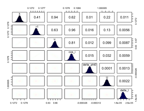
  Figure 1: Pairwise Correlation Diagram of 7 estimated parameters of Kepler-1b. The columns correspond to each of the model parameters, as discussed in Section 2.1 (“The model”), e.g., $k$ is the ratio of the planet radius to the stellar radius, and so on. The pairwise correlation coefficients are in the upper right boxes, e.g., 0.41 for between $r_{1}$ and $k$. The histograms are the distributions for each of the parameters The lower left (below the diagonal) plots the joint distribution between two parameters at a time, giving an insight into the n-dimensional surface being optimised over. The colours correspond to frequency, or the number of times the MCMC was found in this point. Red corresponds to most frequent, and is found in the centre of the distributions, with counts falling away from these points.

• Kepler 2b: The histograms show that the distributions of all parameters are unimodal. The pairwise correlations plots show that $r_{1}$ and $cos(i)$ have the strongest relationship, while the others are less related. All $\hat{R}$ statistics were close to 1.

• Kepler 8b: Again, all parameters have unimodal distributions. The correlations plots suggest that the parameters do not have linear relationships. Convergence was good (see Table 3), but the 95% quantiles are wide, indicating a weak solution.

• Kepler 77b: is similar to Kepler 8b, with wide quantiles but good convergence statistics. Gandolfi et al. (2013) present a more detailed MCMC-based analysis than this paper’s, including radial velocity measurements with Kepler photometry. We note that our paper’s error estimates are an order of magnitude larger than those of Gandolfi et al., for instance they estimate inclination as $88.00\pm 0.11$ degrees and the planet to star radius as $0.09924\pm 0.00026$, with error bars being defined to be at the 68% confidence limits. We plan to revisit Kepler 77b with a more sophisticated model (as discussed above) and see if an improved model leads to a reduction in our error estimates and towards those of Gandolfi et al.

A feature of the HMC fits is just how large the 95% uncertainties from the fitting are, reflecting the difficult nature of ‘untangling’ the various effects we have modelled. The HMC solutions are generally consistent with the model fits before, but now have estimates of the parameter reliability, plus we were able to include $u$ as a free parameter more confidently. Not all the HMC intervals overlap with the intervals constructed from the multiple light curves analyses. The ILOT ‘errors’ for Kepler-1 were similar to the uncertainties from HMC. The HMC result for Kepler-2 was quite different from ILOT, just as ILOT’s solution had been different to those of the other optimisation methods tested at the beginning of this study. HMC also struggled with the Kepler-8 data, giving large uncertainties, as with Kepler-77. We discuss the effect of lowering signal to noise later in the paper. There is also the issue of ‘chi-squared valleys’ or ‘local minima’ — about which some optimization methods ‘handle’ better than others, not getting caught in these secondary minima. MCMC methods are particularly good at such escapes, although as noted above we do not appear to have over-parameterised the transit light curve data and therefore the solution search space appears to be highly convex. The MCMC correlation diagrams confirm this interpretation, along with the not surprising correlations between the three key parameters of planetary radii ($r_{1}$), ratio of the planetary and stellar radii ($k$) and the limb darkening ($u$). These relations with limb darkening somewhat complicated comparisons with the simpler modelling above, and speaks towards the necessity of the more computing intensive method of MCMC to properly explore the search space. As we will see with later systems in this paper, the optima can be more complicated than we expected at this stage of the study. Offset parameters (in phase and flux) were clearly Gaussian, as was the noise (‘delta_l’ in the correlation charts).

The results for Kepler 8 are quite different to the initial estimates, but within the estimated uncertainties. The difference could be due to data treatment (e.g., data folding and binning) as well as the outliers in the multiple light curve results. However, we believe that the HMC estimates are more accurate, given that we only tested 30 light curves in the individual fits above.

System	Parameters	Point Estimate	95% Interval Estimate
Kepler 1b	$k$	0.126	(0.122, 0.128)
…	$r_{1}$	0.121	(0.120, 0.122)
…	$u$	0.638	(0.555, 0.711)
…	$i$	84.238	(84.110, 84.355)
…	$\sigma$	0.000057	(0.000048, 0.000070)
Kepler 2b	$k$	0.0777	(0.0775, 0.0779)
…	$r_{1}$	0.236	(0.235, 0.238)
…	$u$	0.461	(0.451, 0.472)
…	$i$	83.545	(83.293, 83.304)
…	$\sigma$	0.000041	(0.000035, 0.000047)
Kepler 8b	$k$	0.094	(0.090, 0.097)
…	$r_{1}$	0.138	(0.124, 0.156)
…	$u$	0.658	(0.399, 0.811)
…	$i$	84.759	(83.082, 86.244)
…	$\sigma$	0.00044	(0.000037, 0.000052)
Kepler 77b	$k$	0.099	(0.096, 0.104)
…	$r_{1}$	0.112	(0.100, 0.123)
…	$u$	0.558	(0.378, 0.721)
…	$i$	86.863	(85.585, 88.890)
…	$\sigma$	0.00073	(0.00061, 0.00088)

Table 4: Summary of estimated parameters from HMC for Kepler 1b, 2b, 8b, and 77b

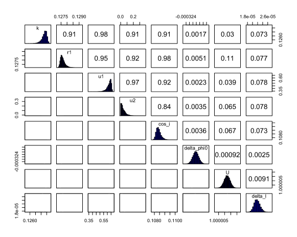
Figure 2: Pairwise Correlation Diagram of 8 estimated parameters of Kepler 1b. $u_{1}$ and $u_{2}$ are parameters for the quadratic limb darkening model

We considered whether to add more detailed modelling of the limb darkening. A test was therefore made using a quadratic limb darkening law for Kepler 1b. The limb darkening coefficients were not well defined (see Table 5 and 6, plus Figure 2). We saw no improvement in going to this model, and so remained with a simple linear model for the remaining fits. Within ILOT philosophy, including more terms in the l.d. expression dilutes the determinacy of individual parameters, even when it does not create a general breakdown of determinacy due to the failure of the Hessian to remain positive definite. And with that, the higher order terms in that expression are expected to be small, or very small, in comparison to their errors.

	$k$	$r_{1}$	$u_{1}$	$u_{2}$	$cos(i)$	$offset$	$U$	$\sigma$
$\hat{R}$	1.037882	1.040101	1.048493	1.052874	1.030407	1	1	1

Table 5: $\hat{R}$ of transit parameters for Kepler 1b with quadratic limb darkening model

Parameters	Point Estimate	95% Interval Estimate
$k$	0.1273	(0.1267, 0.1276)
$r_{1}$	0.1276	(0.1274, 0.1281)
$u_{1}$	0.6220	(0.5394, 0.6612)
$u_{2}$	0.0420	(0.0016, 0.1401)
$i$	83.776	(83.745, 83.797)
$\sigma$	0.00002	(0.00002, 0.00002)

Table 6: Summary of estimated parameters from HMC for Kepler 1b with quadratic limb darkening model

2.3.2 Candidate Systems

The HMC fits on the known systems gave comparable results to the literature and the previous fits in this study. We were therefore confident to apply the model to four ‘new’ systems without published parameters. These are KOI 760.01, 767.01, 802.01, and 824.01. We adopted the NEA orbital periods after confirming that the NEA-assigned periods were reasonable via linear regressions (see Table 7).

The light curves are not as ‘clean’ as the previous systems modelled. KOI 802.01 and 824.01 have relatively long periods, reducing the number of transits available for modelling. There were only 5 transits available for 760.01, 30 for 767.01, 11 for 802.01, and 9 for 824.01. We did model these transits separately, but the ‘error bars’ were large (even $r_{1}$ for 767.01 had a 95% interval range of 0.103 to 0.222, so we decided to go straight through to MCMC modelling.

Before discussing the results, we will briefly consider signal to noise. If we compare transit depth to the noise $\sigma$ it should be no surprise that the S/N (signal to noise) levels are lower for the candidate systems. Kepler 1b has a signal to noise ratio of about 252, 2b 164, 8b 22, and 77b 16. By comparison, the S/N for KOI 760.01 is 7, for 767.01 19, 802.01 2.3 , and 824.01 7. We therefore expected wider ‘uncertainties’ in our results for the candidate systems, and that our parameters would be best defined for KOI 767.01 of all the candidate systems.

• KOI 760.01: Table 8 gives the results of these fits, and for the other three candidate systems. The limb darkening is approximately uniformly distributed, indicating poor definition. Other parameters have unimodal distributions. Only $r_{1}$ and $cos(i)$ have a strong positive correlation. Convergence statistics look good (Table 3) and the chains appear converged. Limb darkening does not seem to be an optimisable variable for this data set.

• KOI 767.01: All parameters are unimodal bar $cos(i)$, which is apparently uniformly distributed. Chains appear well converged.

• KOI 802.01: $r_{1}$ and $u$ can take any values between 0 and 1, indicating that we can not optimise these parameters together with the others. This system has a low signal to noise ratio, so it is not unexpected that modelling will be more problematic.

• KOI 824.01: Similar to KOI 802.01, this system has a low signal to noise ratio. Parameter $u$ can take any values between 0 and 1, indicating that we can not optimise it together with the others.

System	Point Estimate	Standard Error	95% Interval Estimate	NEA
KOI 760.01	4.9597	0.0005	(4.9577, 4.9617)	4.95932
KOI 767.01	2.81659	0.00009	(2.8164, 2.8168)	2.81650
KOI 802.01	19.60	0.01	(19.569, 19.627)	19.62035
KOI 824.01	15.375	0.002	(15.368, 15.382)	15.37563

Table 7: Summary of estimated periods (in days) for 4 ‘new’ systems

System	Parameters	Point Estimate	95% Interval Estimate
Kepler 760.01	$k$	0.1066	(0.1001, 0.1120)
…	$r_{1}$	0.0847	(0.7590, 0.0925)
…	$u$	0.722	(0.0894, 0.9896)
…	$i$	85.888	(85.279, 86.600)
…	$\sigma$	0.0008	(0.0007, 0.0009)
Kepler 767.01	$k$	0.1238	(0.1226, 0.1250)
…	$r_{1}$	0.1176	(0.1152, 0.1199)
…	$u$	0.5234	(0.4724, 0.5704)
…	$i$	86.618	(86.329, 86.921)
…	$\sigma$	0.0005	(0.0004, 0.0006)
Kepler 802.01	$k$	0.1477	(0.1456, 0.1499)
…	$r_{1}$	0.0163	(0.0156, 0.0169)
…	$u$	0.1478	(0.0056, 0.4043)
…	$i$	89.296	(89.247 ,89.352)
…	$\sigma$	0.0062	(0.0060, 0.0064)
Kepler 824.01	$k$	0.1214	(0.1130, 0.1265)
…	$r_{1}$	0.0317	(0.0256, 0.0363)
…	$u$	0.4517	(0.0428, 0.8618)
…	$i$	88.671	(88.299, 89.274)
…	$\sigma$	0.0032	(0.0030, 0.0033)

Table 8: Summary of estimated parameters from HMC for KOI 760.01, 767.01, 802.01, and 824.01

Among the 8 systems, Kepler 1, 2, 8, 77 and KOI 767.01 have S/N above 15. Their corresponding estimates of limb darkening coefficient $u$ have higher determinacy than the others, i.e., the error bars are narrower. Therefore, we have estimated the borderline S/N for limb darkening coefficient to be 15. For noisy data with low S/N, it is preferable to take the limb darkening coefficient derived from appropriate stellar atmosphere models rather than derive it from the data.

We note Csizmadia et al. (2013) made a detailed study of the determinability of limb darkening coefficients. This study created 2000 light curves using the subroutines of Mandel & Agol (2002), assuming a circular orbit and adding levels of Gaussian noise to give different levels of signal to noise (S/N). A genetic optimisation method was then applied to these synthetic light curves, fitting a transit model. Figure 3 of their paper plots the relative uncertainties in derived parameters, including limb darkening, against S/N. They note that a S/N of at least 25 and 6 is required to fit quadratic limb darkening coefficients (i.e., the determinability of the limb darkening coefficients depends on the transit depth relative to the noise). From this figure, it can be seen that the limb darkening co-efficients can be derived subject to an approximately 6% precision if the S/N ratio is 15, in line with the current paper and confirming their results.

We have re-fitted KOI 802.01 (with the lowest S/N) data using 6 parameters, excluding limb darkening coefficient $u$. As for $u$, we have fixed a theoretical value 0.41 determined by winfitter program. See tables 9 and 10.

All six transit parameters for KOI 802.01 have uniform distribution and the fitted light curve looks reasonable. According to tables 9 and 10, the 95% interval estimates are reasonably small for all six parameters and the $\hat{R}$ are all close to 1, suggesting the Markov Chain has converged.

Parameters	Point Estimate	95% Interval Estimate
$k$	0.1482	(0.1457, 0.1508)
$r_{1}$	0.0158	(0.0150, 0.0167)
$i$	89.353	(89.277 ,89.410)
$\sigma$	0.0062	(0.0060, 0.0064)

Table 9: Summary of estimated parameters (excluding $u$) from HMC for KOI 802.01

	$k$	$r_{1}$	$cos(i)$	$offset$	$U$	$\sigma$
$\hat{R}$	1.000733	1.001587	1.001534	1	0.9999253	1

Table 10: $\hat{R}$ of transit parameters for KOI 802.01

We referred to the Kepler Candidate Overview page of KOI 802.01 on the NEA website to check the validity of our fitted results. However, the information in that catalog seem to be inconsistent. According to the “KOI Transit Results” section, we could derive $R\textsubscript{Star}$ (of $R\textsubscript{Sun}$) by applying Kepler’s Third Law. The derived radius is smaller than 0.5R_⊙, consistent with our fitted results. On the other hand, in the Stellar Properties section, $R\textsubscript{Star}$ (in R_⊙) is reported as 0.77 to 0.87(!). Similarly, the effective temperature of the star is given as around 5700 K, which is close to that of the Sun. But for a solar effective temperature, the derived stellar radius in KOI 802 would be too small for any normal star. These findings suggest something unusual in the KOI 802.01 identification. It seems possible that the star identified in the catalog is not the one being eclipsed. Such a scenario might account for the inconsistency between the radius derived from transit curves and from the basis of normal stellar structure models. This question supports the need for further investigation and additional observational data. We confirm this by noting Batalha (2014), who gives useful information on the NEA catalogues and explains that the Kepler Input Catalog (KIC, see Brown et al., 2011 for background on this catalog) provided the stellar properties listed on the site. These are in turn derived from ground-based photometry and modelling. Batalha notes that the KIC “contains known deficiencies and systematic errors, making it unsuitable for computing accurate planet properties” and we urge diligence be taken for stellar parameters case by case, particularly for the fainter and therefore harder to measure stars (the KIC gives a Kepler magnitude of 15.562 for KOI 802, which can be compared with the 11.338 for Kepler-1).

3 Conclusions

This paper has described a simple transit model and its application using a variety of optimisation techniques to fit selected Kepler light curves. The model was first applied to systems with published parameters, deriving point estimates in good agreement with the literature. Provided that the information content of the data is respected, the point estimates were effectively independent of the optimisation method indicating a tidy convex optimisation problem. The following example might make clear our argument against overfitting: a sine wave has four meaningful parameters — amplitude, offset, frequency and a non-zero center amplitude. It is possible to fit additional parameters to a ‘noisy’ sine wave data set, but how to interpret these parameters? Such over-fitting the data can cloud meaningful analysis, and we believe it is extremely important for analysts to keep in mind the information content of the data in analysis, such as through consideration of S/N and its impact on determinability.

A key question in this study was whether limb darkening could be derived from the data sets. We started with a simple linear model, frequently finding indeterminacy when even linear limb darkening was included as an optimisable parameter. The situation did not improve when a quadratic model was applied (we had wondered if the linear model was too much of a simplification and subsequently leading to poor fits), and the MCMC optimisations showed limb darkening to be poorly defined from the data. However this test was only one case. Later work will involve trialling different models and investigating whether statistically robust co-efficients can be derived for Kepler transits (taking note of Espinoza & Jordan (2015) and Espinoza & Jordan (2016)). The MCMC fits above clearly showed correlations between limb darkening and a key variable of interest in exoplanets: the radius of the exoplanet itself. We therefore believe that continued modelling and exploration of the confidence in limb darkening estimates across different models, systems, and across different periods (for those systems) is an important task. Exoplanet transit light curves provide a ‘laboratory’ for exploration of limb darkening, allowing refinement of our stellar models (see also Csizmadia et al. , 2013).

Such an investigation will require improvement to the rather simple model used in this paper, ensuring that we have removed other physics before trying to fit limb darkening models. We further intend to improve the fitting model, noting the deficiencies described earlier in the paper such as use of the small planet approximation, and continue our investigation into the parameter distributions of model fits to the Kepler data.

Such an improved model will also allow better comparison with results from winfitter, which is a more sophisticated model. The comparisons between winfitter and MCMC in this paper have, unfortunately, been inconclusive. We have not really been comparing “like with like”. As noted above, winfitter uses an optimized chi-square fit of the light curve to the physical parameters of the system such as mass, luminosity, period and separation. It is much faster in computer run times than MCMC, and if it can be shown that its estimates of the accuracy of parameters are consistent with MCMC, then it would be a useful tool for parameterising transit light curves, particularly at large scale (i.e., an automated system running across large data sets of multiple systems). winfitter includes the relevant proximity effects such as radiative interaction (reflection effects), tidal and rotational distortions, gravity brightening (ellipticity effects), limb darkening, Doppler beaming effect, and orbital eccentricity (if present). A further advantage of winfitter is that it also produces a distortion-wave light curve that is the difference between the observed and model light curves. This ‘difference curve’ can then be analyzed by spotfitter, an ILOT based starspot modeling application, which uses a circular, dark starspot model to find the latitude, longitude, size and temperature of one or two spot groups on the active primary star.

We believe that knowledge of such parameter distributions will be important for any ‘meta-analyses’ based on collection of many individual and separate studies deriving exoplanet parameters. This is why we have kept the distribution charts in this paper, and we encourage other researchers to share their ‘uncertainties’. Without a clear understanding of confidence limits in modelling results, meta-analyses might reach incorrect conclusions by placing undue weight on ‘observations’ of dubious confidence or indeed the reverse. We strongly encourage other researchers in the field to use techniques such as MCMC to explore the determinacy of their model fit and the confidence that should be placed in the parameter estimates.

4 Acknowledgements

This research has made use of the NASA Exoplanet Archive, which is operated by the California Institute of Technology, under contract with the National Aeronautics and Space Administration under the Exoplanet Exploration Program. It is a pleasure to acknowledge the additional help and encouragement from the National University of Singapore, particularly through Prof. Lim Tiong Wee of the Department of Statistics and Applied Probability. Associate Professor Alex R. Cook and Associate Professor David Nott provided valuable guidance on the Random Walk Metropolis-Hastings and Hamiltonian Monte Carlo (HMC) applications. winfitter is available at http://michaelrhodesbyu.weebly.com/astronomy.html

References

- akeson (2013) Akeson, R.L., Chen, X., Ciardi, D., Crane, M., Good, J., Harbut, M., Jackson, E., Kane, S.R., Laity, A.C., Leifer, S., Lynn, M., McElroy, D. L., Papin, M., Plavchan, P., Ramirez, S.V., Rey, R., von Braun, K., Wittman, M. , Abajian, M., Ali, B., Beichman, C., Beekley, A., Berriman, G.B., Berukoff, S., Bryden, G., Chan, B., Groom, S., Lau, C., Payne, A. N., Regelson, M., Saucedo, M., Schmitz, M., & Stauffer, J., Wyatt, P., & Zhang, A., PASP, 125, 989, 2013
- albert (2014) Albert, J., 2014, “LearnBayes: Functions for Learning Bayesian Inference”, https://CRAN.R-project.org/ package=LearnBayes
- Ballard (2014) Ballard, S., et al. (25 authors), 2014, Astrophysical Journal, 790, 12
- Banks (1990) Banks, T., & Budding, E., 1990, Ap&SS, 167, 221
- Banks2 (1990) Banks, T., Sullivan, D.J., & Budding, E., 1990, Ap&SS, 173, 77
- Banks2 (1991) Banks, T., Kilmartin, P.M., & Budding, E., 1991, Ap&SS, 183, 309
- Banks3 (1994) Banks, T., Dodd, R.J., & Sullivan, D.J., 1994, MNRAS, 272, 821
- Banks4 (1995) Banks, T., Sullivan, D.J., & Dodd, R.J., 1995, MNRAS, 274, 1225
- Batalha (2014) Batalha, N. M., 2014, PNAS, 111 (35), 12647
- Bertsimas (1993) Bertsimas, D., & Tsitsiklis, J., 1993, Statistical Science, 8, 10-15
- Bevington (1969) Bevington, P.R., 1969, Data Reduction and Error Analysis for the Physical Sciences, McGraw-Hill, New York
- Borucki (2003) Borucki, W.J., et al. (14 authors), 2003, in Scientific Frontiers in Research on Extrasolar Planets, Eds. D. Deming and S. Seager, ASP Conf. Ser. 294, 427
- (13) Borucki, W.J., et al. (69 authors), 2011, ApJ, 736, 19
- Brooks (1997) Brooks, S., & Gelman, A., 1997, J. Comput. Graph. Statist, 434
- Brooks (2011) Brooks, S., Gelman, A., Jones, G., & Meng, X., 2011, Handbook of Markov Chain Monte Carlo, Chapman and Hall, CRC
- brown (2011) Brown, T. M., Latham, D. W., Everett, M. E., & Esquerdo, G. A., 2011, Ap. J, 142, 112
- Budding (2007) Budding, E., & Demircan, O., 2007, Introduction to Astronomical Photometry, CUP
- Budding (2016a) Budding, E., Püsküllü, Ç., Rhodes, M.D., Demircan, O., & Erdem, A., 2016, Ap&SS, 361, 17
- Budding (2016b) Budding, E., Rhodes, M.D., Püsküllü, Ç., Ji, Y., Erdem, A., & Banks, T., 2016, Ap&SS, 361, 346
- Charbonneau (1999) Charbonneau, D., Noyes, R.W., Korzennik, S.G., Nisenson, P., Jha, S., Vogt, S.S., & Kibrick, R.I., 1999, ApJ, 527, 445
- Ciupke (2016) Ciupke, K., 2016, “psoptim: Particle Swarm Optimization”, https://CRAN.R-project.org/package=psoptim
- Cortez (2014) Cortez, P., 2014, Modern Optimization with R (1st Edition ed.), Springer, Switzerland.
- Csizmadia (2013) Csizmadia, Sz., Pasternacki, Th., Dreyer, C., Cabrera, J., Erikson, A., & Rauer, H., 2013, A&A, 549, A9
- Elzhov (2016) Elzhov, T.V., Mullen, K. M., Spiess, A. N, & Bolker, B., 2016, “minpack.lm: R Interface to the Levenberg-Marquardt Nonlinear Least-Squares Algorithm Found in MINPACK, Plus Support for Bounds”, https://CRAN.R-project.org/package=minpack.lm
- Espinoza (2015) Espinoza, N., & Jordan, A., 2015, MNRAS, 450, 1879
- Espinoza (2016) Espinoza, N., & Jordan, A., 2016, MNRAS, 457, 3573
- Ford (2005) Ford, E. B., 2005, AJ, 129, 1706
- Gandolfi (2013) Gandolfi, D., Parviainen, H., Fridlund, M., Hatzes, A. P., Deeg, H. J., Frasca, A., Lanza, A.F., Prada Moroni, P. G., Tognelli, E., McQuillan, A., Aigran, S., Alonso, R., Antoci, V., Cabrera, J., Carone, L., Csizmadia, Sz., Djupvik, A. A., Guenther, E.W., Jessen-Hansen, J., Ofir, A., & Telting, J., 2013, A&A, 557, A74
- Gelman (1992) Gelman, A., & Rubin, D. B., 1992, Statistical Science 7, 457
- Givens (2011) Givens, G.H., & Hoeting, J. A., 2013, Computational Statistics - 2nd Edition’, Wiley
- Mandel (2002) Mandel, K., Agol, E., 2002, ApJ, 580, 171
- Mitchell (1998) Mitchell, M., 1998, “An Introduction to Genetic Algorithms (Complex Adaptive Systems)”, MIT Press
- Moutou (2013) Moutou, C., Deleuil, M., Guillot, T., Baglin, A., Bord , P., Bouchy, F., Cabrera, J., Csizmadia, S., & Deeg, H.J., 2013, Icarus, 226, 1625
- Mullaly (2015) Mullally, F., Coughlin, J. L., Thompson, S. E., et al. 2015, ApJS, 217, 31
- Nutzman (2009) Nutzman, P., Charbonneau, D., Winn, J. N., Knutson, H.A., Fortney, J.J., Holman, M. J., & Agol, E., Ap. J., 692, 229, 2009
- Pollacco (2006) Pollacco, D.L., et al. (27 authors), 2006, PASP, 118, 1407
- Pont (2006) Pont, F., Zucker, S., & Queloz, D., MNRAS, 2006, 373, 231
- RCore (2014) R Core Team, 2014, R: A language and environment for statistical computing, R Foundation for Statistical Computing, Vienna, Austria.
- rhodes (2014) Rhodes, M.D., & Budding, E., 2014, ApSS, 351: 451
- Rice (2014) Rice, K., 2014, Challenges, 5, 296
- Ricker (2010) Ricker, G. R., Latham, D. W., Vanderspek, R. K., Ennico, K. A., Bakos, G., Brown, T. M., Burgasser, A. J., Charbonneau, D., Clampin, M., Deming, L. D., Doty, J. P., Dunham, E. W., Elliot, J. L., Holman, M. J., Ida, S., Jenkins, J. M., Jernigan, J. G., Kawai, N., Laughlin, G. P., Lissauer, J. J., Martel, F., Sasselov, D. D., Schingler, R. H., Seager, S., Torres, G., Udry, S., Villasenor, J. N., Winn, J. N., & Worden, S. P., American Astronomical Society, AAS Meeting #215, id.450.06; Bulletin of the American Astronomical Society, Vol. 42, 459
- Rini (2011) Rini, D.P., Shamsuddin, S.M., & Yuhaniz, S.S., 2011, International Journal of Computer Applications, 14, 19
- Rowe (2014) Rowe, J. F., Bryson, S. T., Marcy, G. W., et al. 2014, ApJ, 784, 45
- Sinharay (2003) Sinharay, S., 2003, Assessing Convergence of the Markov Chain Monte Carlo Algorithm: A Review, ETS Research Report Series, i-52.
- Sobolev (1975) Sobolev, V.V., 1975, Light Scattering in Planetary Atmospheres, Pergamon Press, Oxford
- Stan (2016) Stan Development Team, 2016, “RStan: the R interface to Stan”, http://mc-stan.org/
- Tenenbaum (2010) Tenenbaum, P., Brysona, S. T., Chandrasekarana, H., Jie, L, Quintanaa, E., Twickena, J. D., & Jenkinsa, J. M., 2010, Proc. SPIE, 7740
- Wang (2013) Wang, Z., Mohamed, S., & de Freitas, N., 2013, Adaptive Hamiltonian and Riemann Manifold Monte Carlo Samplers, In: International Conference on Machine Learning (ICML), JMLR W&CP, 28(3), 1462
- Xiang (2013) Xiang, Y., Gubian, S., Suomela, B., & Hoeng, J., 2013, “Generalized Simulated Annealing for Efficient Global Optimization: the GenSA Package for R”, The R Journal, Volume 5/1, URL http://journal.r-project.org/
- Zielik (1988) Zeilik, M., DeBlasi, C., Rhodes, M., & Budding, E., 1988, Astrophys. J. 332, 293
- Zeilik (1994) Zeilik, M., Gordon, S., Jaderlund, E., Ledlow, M. J., Summers, D. L., Heckert, P. A., Budding, E., & Banks, T., 1994, Astrophys. J, 421, 303