Majorana-Hubbard model on the square lattice

Abstract

We study a tight-binding model of interacting Majorana (Hermitian) modes on a square lattice. The model may have an experimental realization in a superconducting-film–topological-insulator heterostructure in a magnetic field. We find a rich phase diagram, as a function of interaction strength, including an emergent superfluid phase with spontaneous breaking of an emergent $U(1)$ symmetry, separated by a supersymmetric transition from a gapless normal phase.

I Introduction, model, and Phase diagram

The discovery of topological materials [König et al., 2007; Zhang et al., 2009; Xia et al., 2009; Mourik et al., 2012] has led to great interest in Majorana modes (MM) [Alicea, 2012; Beenakker, 2013], which are promising candidates for topological quantum computing [Nayak et al., 2008; Hyart et al., 2013; Aasen et al., 2016; Karzig et al., 2016]. The MM’s are predicted to appear in various situations at topological defects and boundaries of topological superconductors [Kitaev, 2001; Fu and Kane, 2008; Lutchyn et al., 2010; Oreg et al., 2010]. In addition to theoretical proposals (and subsequent experimental progress) for realizing a separated localized MM  [Fu and Kane, 2008; Lutchyn et al., 2010; Oreg et al., 2010; Mourik et al., 2012; Albrecht et al., 2016], in certain situations, in both one and two dimensions, a finite density of MM’s is expected  [Fu and Kane, 2008; Zhou et al., 2013; Biswas, 2013; Chiu et al., 2015; Liu and Franz, 2015; Pikulin et al., 2015]. The effects of interactions between MM’s in such setups is a relatively unexplored field [Hermanns and Trebst, 2014; Chiu et al., 2015; Pikulin et al., 2015; Rahmani et al., 2015a, b; Milsted et al., 2015; Witczak-Krempa and Maciejko, 2016; Ware et al., 2016]. Interaction effects have also been studied [Gangadharaiah et al., 2011; Lobos et al., 2012] in the Kitaev model [Kitaev, 2001] in which two localized Majorana modes appear at the ends of a chain. The corresponding Hamiltonians are Hubbard-like (with Majorana fermions serving as Hermitian counterparts of electrons), but necessarily have interactions spanning at least four lattice sites, since the square of a Majorana operator is a constant.

The simplest such model, defined on a chain, was shown to have a rich phase diagram, with four different phases [Rahmani et al., 2015a, b; Milsted et al., 2015]. The continuum limit involved a single species of massless relativistic Majorana fermions and interactions that are irrelevant when weak enough, since interactions necessarily contain derivatives of the Majorana fields. At strong enough coupling, MM’s like to pair up on neighboring sites to form ordinary Dirac (non-Hermitian) fermions, leading to spontaneously broken translation symmetry due to the dimerization. The transition into this broken symmetry phase for attractive interactions was shown to be described by the tricritical Ising model, which exhibits supersymmetry. A phase with emergent $U(1)$ symmetry was also found at intermediate strength repulsive interactions, corresponding to a Luttinger liquid plus a relativistic Majorana fermion. Stronger repulsive interactions again led to Majorana fermions combining on neighboring sites to form Dirac fermions but in this case there is a further breaking of translational symmetry.

Figure 1: The mean-field phase diagram for $t=1$ and $t_{2}=0$ as a function of $g$. The solid (dashed) lines represent second-order (first-order) transitions. The broken symmetry states are sketched in Figs. (2, 8, and 12).

In this paper, we study a two-dimensional model of interacting Majorana modes, motivated by a possible experimental realization in a superconducting thin film placed in a perpendicular magnetic field on top of a strong three-dimensional topological insulator. For simplicity, we consider the case of a square lattice of vortices, with each of them containing a Majorana mode. Requiring one superconducting flux quantum at each vortex determines the signs of the hopping terms to be  [Grosfeld and Stern, 2006; Liu and Franz, 2015]

$$H_{0}=it\sum_{m,n}\gamma_{m,n}[(-1)^{n}\gamma_{m+1,n}+\gamma_{m,n+1}],$$ (1)

up to a $\mathbb{Z}_{2}$ gauge transformation, where $n$ and $m$ are integers. (The sign alternation of the horizontal hopping term can be changed by a gauge transformation but sign alternation cannot be completely removed.) We include the shortest possible range interaction term, occurring on plaquettes:

$$H_{int}=g\sum_{m,n}\gamma_{m,n}\gamma_{m+1,n}\gamma_{m+1,n+1}\gamma_{m,n+1}.$$ (2)

We expect [Chiu et al., 2015] the actual interactions between Majorana modes to exhibit exponential decay; this short-range interaction, analogous to the Hubbard interaction for complex fermions, is a convenient simplification. The sign of $g$ is linked to the gauge choice in $H_{0}$ and the sign of the underlying physical interaction. We also discuss the effects of a second-neighbor hopping term chosen to be consistent with the flux:

$$H_{2}=it_{2}\sum_{m,n,s,s^{\prime}}\gamma_{m,2n}\gamma_{m+s,2n+s^{\prime}}$$ (3)

where $s$ and $s^{\prime}$ are summed over $\pm 1$. The Majorana operators are Hermitian,

$$\gamma_{m,n}=\gamma_{m,n}^{\dagger}$$ (4)

and obey the anti-commutation relations:

$$\{\gamma_{m,n},\gamma_{m^{\prime},n^{\prime}}\}=2\delta_{m,m^{\prime}}\delta_{n,n^{\prime}},$$ (5)

implying $\gamma_{m,n}^{2}=1$. Note that this model has no conserved particle number so no chemical potential can be introduced. The sign of $t$ can be changed by sign redefinitions of the $\gamma$’s; we choose $t>0$. There is thus only one dimensionless parameter, $g/t$, in the model. An accurate numerical treatment of this model is an enormous challenge, similar to the Hubbard model, and we do not attempt it here. Instead, we tackle the model with a combination of field theory, renormalization group and mean-field approaches. A promising numerical approach may be density-matrix renormalization group calculations on ladders [Zhu and Franz, 2016]; we will present results on this in a later paper. Note that this model is fundamentally different and much more challenging to study than other lattice models involving two copies of Majorana fermions, which are actually equivalent to ordinary complex fermion models, and have a conserved particle number [Hayata and Yamamoto, 2017]. Unlike the model of Refs. [Li et al., 2015; Hayata and Yamamoto, 2017], our model does not appear to be amenable to Quantum Monte Carlo simulations. As in the 1D works [Rahmani et al., 2015a, b], we study the model for both signs of the coupling constant. It is not completely clear which sign of the interactions might occur in experiments due to the effectively attractive interactions in a superconductor. $g>0$ corresponds to attractive interactions, as we will see.

We find the following mean-field phase diagram, when $t_{2}=0$, sketched in Fig. 1:

• For $0<g<g_{c4}$, there is a gapless phase with broken $\pi/2$ rotation symmetry. This phase has an emergent conserved particle number, $U(1)$, symmetry. There is also an emergent Lorentz invariance, upon rescaling the $x$-coordinate.

• For $g>g_{c4}$, the emergent $U(1)$ symmetry is spontaneously broken at the critical point $g_{c4}$, corresponding to an emergent superfluid phase.

• For $g_{c3}<g<0$, there is a gapless phase with no broken symmetries. This phase has several emergent symmetries including Lorentz invariance and an emergent conserved particle number, $U(1)$, symmetry. The phase transition at $g=0$ is first order.

• For $g_{c2}<g<g_{c3}$, there is a phase with spontaneously broken parity and time reversal. The phase transition is second order (first order) at $g_{c3}$ ($g_{c2}$).

• For $g_{c1}<g<g_{c2}$, there is a phase with spontaneously broken $\pi/2$ spatial rotation symmetry. This phase has translation symmetry in the diagonal direction.

• For $g<g_{c1}$, we have a phase that in addition to the $\pi/2$ spatial rotation, also breaks the diagonal translation symmetry. The transition at $g_{c1}$ is first order.

The broken symmetry phases occurring for $g<g_{c2}$ and $g>g_{c4}$ correspond to nearby Majorana modes combining in pairs to form Dirac fermions, in different patterns. The transition at $g_{c4}$ between gapless and emergent superfluid phases is in a ${\cal N}=2$ supersymmetric (SUSY) universality class [Thomas, 2005; Lee, 2007; Ponte and Lee, 2014; Jian et al., 2015; Zerf et al., 2016]. (This is distinct from other condensed matter realizations of ${\cal N}=1$ SUSY [Grover et al., 2014].) A nonzero $t_{2}$ produces a gap in the weak coupling phase, corresponding to a mass in the field theory. A transition to an emergent superfluid phase still occurs for large enough positive $g$ but we expect that it is now in the conventional $U(1)$ universality class, without supersymmetry. A nonzero $t_{2}$ explicitly breaks parity and time reversal, eliminating the transition at $g_{c3}$. The phases for $g<g_{c2}$ with spontaneously broken spatial rotation symmetry may still occur.

The remainder of this paper is organized as follows. In Sec. II we analyze the symmetries of the model. In Sec. III we solve the noninteracting model and discuss the topological classification of various phases. In Sec. IV, we derive the low-energy effective field theory and discuss the various emergent symmetries. In Sec. V, we analyze the effects of interactions in mean field theory. In Sec. VI, we discuss the broken symmetry phases using the low energy field theory, and the universality class of the continuous transitions at $g_{c3}$ and $g_{c4}$. We close the paper in Sec. VII with a brief summary.

II Symmetries of the lattice Hamiltonian

The Hamiltonian has no continuous symmetries (in particular, no particle number conservation due to the Majorana nature of the fermions). However, it has 5 important discrete symmetries when $t_{2}=0$, which lead to continuous emergent symmetries in the low energy effective Hamiltonian.

The model, with the second-neighbor hopping included, is invariant under translation by 1 site in the $x$ or $y$ directions:

$$\gamma_{m,n} \to \gamma_{m+1,n}$$

$$\gamma_{m,n} \to (-1)^{m}\gamma_{m,n+1}.$$ (6)

Without second neighbor hopping, the lattice Hamiltonian is invariant under the anti-unitary time reversal transformation, $T$:

$$\gamma_{m,n} \to (-1)^{m+n}\gamma_{m,n}$$

$$i \to -i.$$ (7)

Time reversal symmetry is broken by the next-neighbor hopping term, $\propto t_{2}$. Since our model describes a system in a magnetic field, we expect time reversal symmetry to be broken so there is no reason to exclude $t_{2}$. However, we might hope that it is relatively small compared to $t_{1}$ so that time reversal is an approximate symmetry.

The spatial parity symmetry, reflection in the $x$ axis, is

$$\gamma_{m,n}\to(-1)^{m}\gamma_{-m,n}.$$ (8)

This can be seen to be a symmetry of the Hamiltonian only when second neighbor hopping, $t_{2}$ is excluded. The product of time reversal and parity is a symmetry even when second-neighbor hopping is included.

Finally, the Hamiltonian, including the second-neighbor hopping, is invariant under a $\pi/2$ spatial rotation:

$$\gamma_{m,n}\to s_{m,n}\cdot\gamma_{-n,m}$$ (9)

where

$$s_{m,n} = -1\ \ (m\ \hbox{even}\ \hbox{and}\ n\ \hbox{odd})$$ (10)

$$= 1\ \ (\hbox{otherwise}).$$

This is confirmed in Appendix A.

III Solution of noninteracting model

III.1 The energy spectrum

For the gauge chosen in (1) there are 2 sites per unit cell in the $y$-direction, with $n$ even and odd. We relabel

$$\gamma_{m,2n} = \gamma^{e}_{m,2n},$$

$$\gamma_{m,2n+1} = \gamma^{o}_{m,2n}.$$ (11)

Then we Fourier transform, imposing periodic boundary conditions:

$$\gamma^{e/o}_{\vec{k}}\equiv{1\over\sqrt{2WL}}\sum_{m,n}e^{-i(mk_{x}+2nk_{y})}\gamma^{e/o}_{m,2n}$$ (12)

with

$$\vec{k}=(2\pi r/L,\pi s/W),$$ (13)

for integers $r$ and $s$. $m$ and $n$ run over $L$ and $W$ integer values, respectively, where $L$ and $2W$ are the length and width of the lattice in $x$ and $y$ directions, respectively. $k_{x}$ is between $-\pi$ and $\pi$ while $k_{y}$ is between $-\pi/2$ and $\pi/2$. This gives

$$\{\gamma^{e/o}_{\vec{k}},\gamma^{e/o}_{\vec{k}^{\prime}}\}=\delta_{\vec{k},-\vec{k}^{\prime}}.$$ (14)

Inverting Eq. (12), we find

$$\gamma^{e/o}_{\vec{r}}=\sqrt{2\over WL}\sum_{\vec{k}}e^{i\vec{k}\cdot\vec{r}}\gamma^{e/o}_{\vec{k}},$$ (15)

where $\vec{r}=(m,2n)$.

The Hermiticity of $\gamma^{e/o}_{\vec{r}}$ implies that

$$\gamma^{e/o}_{-\vec{k}}={\gamma^{\dagger}}^{e/o}_{\vec{k}}.$$ (16)

We can then write the noninteracting Hamiltonian (1) as

$$H_{0}=2it\sum_{\vec{k}}[(\gamma^{e}_{-\vec{k}}\gamma^{e}_{\vec{k}}-\gamma^{o}_{-\vec{k}}\gamma^{o}_{\vec{k}})e^{ik_{x}}+\gamma_{-\vec{k}}^{e}\gamma^{o}_{\vec{k}}(1-e^{-2ik_{y}})].$$ (17)

Using Eq. (16), we then obtain

$$\begin{split}H_{0}=2it\sum_{k_{x}>0}[&(\gamma^{e\dagger}_{\vec{k}}\gamma^{e}_{\vec{k}}-\gamma^{o\dagger}_{\vec{k}}\gamma^{o}_{\vec{k}})(e^{ik_{x}}-e^{-ik_{x}})\\ &+\gamma_{\vec{k}}^{e\dagger}\gamma^{o}_{\vec{k}}(1-e^{-2ik_{y}})-\gamma_{\vec{k}}^{o\dagger}\gamma^{e}_{\vec{k}}(1-e^{2ik_{y}})],\end{split}$$ (18)

where a constant was dropped. Diagonalizing the noninteracting Hamiltonian (18) gives the dispersion relation

$$E_{\pm}=\pm 4t\sqrt{\sin^{2}k_{x}+\sin^{2}k_{y}}.$$ (19)

There are Dirac points at $\vec{k}=(0,0)$ and $(\pi,0)$ with two species of massless relativistic fermions in their vicinity, i.e., $E_{\pm}=\pm 4t|\vec{k}|$, with the momentum measured from the Dirac points. Note that we must restrict to $0\leq k_{x}\leq\pi$ and $-\pi/2\leq k_{y}\leq\pi/2$.

The second neighbor hopping adds a term:

$$H_{2}=8it_{2}\sum_{k_{x}>0}\cos k_{x}\cos k_{y}[e^{-ik_{y}}\gamma^{e\dagger}_{\vec{k}}\gamma^{o}_{\vec{k}}-e^{ik_{y}}\gamma^{o\dagger}_{\vec{k}}\gamma^{e}_{\vec{k}}],$$ (20)

which changes the dispersion relation to

$$E_{\pm}=\pm\sqrt{(4t\sin k_{x})^{2}+(4t\sin k_{y})^{2}+(8t_{2}\cos k_{x}\cos k_{y})^{2}}.$$ (21)

Therefore, near the Dirac points, we obtain a massive relativistic dispersion relation:

$$E_{\pm}=\pm\sqrt{(4t)^{2}(k_{x}^{2}+k_{y}^{2})+(8t_{2})^{2}},$$ (22)

where the momenta are measured from the Dirac points.

III.2 Topological classification

To perform the analysis of the topological invariant of the Hamiltonian, Eqs. (18) and (21), we rewrite the total Hamiltonian in the matrix form:

$$H=\begin{pmatrix}\gamma^{e{\dagger}}_{k}\\ \gamma^{o{\dagger}}_{k}\end{pmatrix}\mathcal{H}\begin{pmatrix}\gamma^{e}_{k}&\gamma^{o}_{k}\end{pmatrix},$$ (23)

where

$$\mathcal{H}=d_{x}(k)\sigma^{x}+d_{y}(k)\sigma^{y}+d_{z}(k)\sigma^{z}.$$ (24)

Here $\sigma$’s are the usual Pauli matrices and

$$d_{x}(k) =4t\sin k_{y}\cos k_{y}+8t_{2}\cos k_{x}\cos k_{y}\sin k_{y},$$ (25)

$$d_{y}(k) =4t\sin^{2}k_{y}-8t_{2}\cos k_{x}\cos^{2}k_{y},$$ (26)

$$d_{z}(k) =4t\sin k_{x}.$$ (27)

Phase transitions in the noninteracting model can be understood in terms of the closing of the spectral gap of $\mathcal{H}$. The energy (21) can only vanish at $t_{2}=0$ and $k_{x}=0,\pi$, $k_{y}=0$ in the allowed range of the momenta. Thus there are two Majorana gap closings for $t_{2}=0$, which should correspond to a change of the topological invariant by $2$.

We now proceed to computing the Chern number, $\mathcal{C}$, of Eq. (24), which is

$$\mathcal{C}=\frac{1}{4\pi}\int d^{2}k\frac{1}{|d(k)|^{3}}\mathbf{d}(k)\cdot\frac{\partial\mathbf{d}(k)}{\partial k_{x}}\times\frac{\partial\mathbf{d}(k)}{\partial k_{y}}.$$ (28)

Here the integration goes over the whole Brillouin zone. Explicit integration in this formula gives $+1$ for $t_{2}/t<0$, and $-1$ for $t_{2}/t>0$. The $t_{2}=0$ transition is thus topological with Chern number change of $\pm 2$. Such a phase transition hosts two Majorana cones, in accordance with the gap closing analysis above. We thus conclude that the $t_{2}=0$ point is a topological transition gapless point between $\mathcal{C}=\pm 1$ phases.

The gapped phases for $t_{2}\neq 0$ are analogues of the $p\pm ip$ superconductors, or superconducting analogues of the quantum Hall phases with chiral Majorana (instead of complex fermion) modes at the edges. It is known that the Chern number classification survives in presence of interactions [Wen, 2004], therefore the analysis of the interacting Hamiltonian with $t_{2}=0$ is equivalent to analyzing a topological transition between $\mathcal{C}=\pm 1$ topological superconducting phases.

IV Low Energy Effective Field Theory and its Emergent Symmetries

IV.1 Low-energy Hamiltonian

We start with the $t_{2}=0$ noninteracting Hamiltonian $H_{0}$. Keeping only Fourier modes near the two gapless points, we write:

$$\gamma^{e/o}_{\vec{r}}\approx 2\sqrt{2}[\chi^{e/o+}(\vec{r})+(-1)^{x}\chi^{e/o-}(\vec{r})],$$ (29)

where $\chi^{e/o\pm}(\vec{r})$ vary slowly. [The $2\sqrt{2}$ factor in Eq. (29) is derived in Appendix B.] This gives the anticommutators:

$$\{\chi^{i}(\vec{r}),\chi^{j}(\vec{r}^{\prime})\}={1\over 2}\delta^{ij}\delta^{2}(\vec{r}-\vec{r}^{\prime}),$$ (30)

where $i$, $j$, label the four species of fermions, $\pm$, $e/o$. [This normalization of the anti-commutators is convenient because the relativistic Langrangian density is consequently unit normalized.]

Expanding to first order in derivatives, and using $\sum_{m,n}f(m,2n)\to{1\over 2}\int dxdyf(x,y)$, we find $H_{0}\approx\int dxdy{\cal H}_{0}$ with

$$\begin{split}{\cal H}_{0}=4it\sum_{\pm}\{\pm&[\chi^{e\pm}\partial_{x}\chi^{e\pm}-\chi^{o,\pm}\partial_{x}\chi^{o\pm}]\\ &+\chi^{e\pm}\partial_{y}\chi^{o\pm}+\chi^{o\pm}\partial_{y}\chi^{e\pm}\}.\end{split}$$ (31)

Combining $\chi^{e\pm}$ and $\chi^{o\pm}$ into 2-component spinors, $\vec{\chi}^{+}\equiv(\chi^{e+},\chi^{o+})^{T}$, $\vec{\chi}^{-}\equiv(\chi^{o-},\chi^{e-})^{T}$, we can write

$${\cal H}_{0}=4it\sum_{\pm}\vec{\chi}^{T\pm}\cdot[\sigma^{z}\partial_{x}+\sigma^{x}\partial_{y}]\vec{\chi}^{\pm}.$$ (32)

Going back to momentum space, we can diagonalize the Hamiltonian in terms of the low energy fields. The Majorana nature of the fields implies $\vec{\chi}_{-\vec{k}}^{\pm}=\vec{\chi}^{\pm\dagger}_{\vec{k}}$. The Hamiltonian for the $\chi^{+}$ field, dropping the superscript, becomes

$$H_{0}=v\int_{k_{x}>0}d^{2}k[\chi^{\dagger}_{\vec{k},>}\chi_{\vec{k},>}-\chi^{\dagger}_{\vec{k},<}\chi_{\vec{k},<}]|\vec{k}|,$$ (33)

with the velocity $v=4t$, and $\chi_{\vec{k},>}$ ($\chi_{\vec{k},<}$) representing the eigenmodes with positive (negative) energy. Now it is convenient to make a particle-hole transformation for the negative energy operators:

$$\chi_{\vec{k},<}\to\chi^{\dagger}_{-\vec{k},<}.$$ (34)

The sign change $\vec{k}\to-\vec{k}$ indicates that annihilating a fermion of momentum $\vec{k}$ changes the momentum by $-\vec{k}$. The Hamiltonian can then be written as

$$H_{0}=v\int_{k_{x}>0}d^{2}k[\chi^{\dagger}_{\vec{k},>}\chi_{\vec{k},>}+\chi^{\dagger}_{-\vec{k},<}\chi_{-\vec{k},<}]|\vec{k}|.$$ (35)

As we are now covering the entire $\vec{k}$-space, with both signs of $k_{x}$, we may drop the subscripts and simply write:

$$H=v\int d^{2}k\chi^{\dagger}_{\vec{k}}\chi_{\vec{k}}|\vec{k}|,$$ (36)

which is the standard result for a Majorana fermion. There are particle excitations for all values of $\vec{k}$ and no antiparticle states. The interaction term can also be readily written in terms of the low-energy degrees of freedom as

$${\cal H}_{int}=256g\chi^{e-}\chi^{e+}\chi^{o+}\chi^{o-}.$$ (37)

Finally, in the low-energy theory, the second-neighbor hopping term becomes:

$${\cal H}_{2}=16it_{2}[\chi^{e+}\chi^{o+}-\chi^{e-}\chi^{o-}].$$ (38)

IV.2 Emergent Lorentz symmetry

We now check that the above Hamiltonian is indeed Lorentz invariant. The Lagrangian density can be written as

$${\cal L}_{0}=i\sum_{\pm}{\vec{\chi}}^{T,\pm}\cdot\partial_{t}{\vec{\chi}}^{\pm}-{\cal H}_{0}={\cal L}_{0,+}+{\cal L}_{0,-}.$$ (39)

The Lagrangian densities ${\cal L}_{0,\pm}$ depend on the chiral fields ${\vec{\chi}}^{\pm}$ as

$${\cal L}_{0,\pm}=i\vec{\chi}^{T,\pm}\cdot\partial_{t}\vec{\chi}^{\pm}-4it\vec{\chi}^{T\pm}\cdot[\sigma^{z}\partial_{x}+\sigma^{x}\partial_{y}]\vec{\chi}^{\pm}$$ (40)

We define the Dirac $\gamma$-matrices

$$\gamma^{\mu}\equiv(\sigma^{y},-i\sigma^{x},i\sigma^{z}),$$ (41)

such that the anticommutator $\{\gamma^{\mu},\gamma^{\nu}\}=2\eta^{\mu\nu}\openone$, with $\eta^{\mu\nu}={\rm diag}(1,-1,-1)$ and $\openone$ is the $2\times 2$ identity matrix. We further define

$$\bar{\chi}\equiv\vec{\chi}^{T}\gamma^{0}$$ (42)

for each of the chiral fields. We also simplify the notation by using $\chi$ instead of $\vec{\chi}$. Suppressing the $\pm$ superscript, the chiral Lagrangian densities take the form

$${\cal L}_{0}=i\bar{\chi}\gamma^{\mu}\partial_{\mu}\chi,$$ (43)

where we have set the velocity, $v=4t$, to one. The above Lagrangian density is invariant under a Lorentz transformation:

$$\chi\to e^{i\gamma^{\mu}a_{\mu}/2}\chi,$$ (44)

which is not unitary in general. In the special case where only $a_{0}\neq 0$, this becomes:

$$\begin{split}\bar{\chi}\gamma^{\mu}\partial_{\mu}\chi\to\bar{\chi}e^{-i\sigma^{y}a_{0}/2}\gamma^{\mu}e^{i\sigma^{y}a_{0}/2}\partial_{\mu}\chi=i\bar{\chi}[\gamma^{0}\partial_{t}+\gamma^{1}(\cos a_{0}\partial_{x}-\sin a_{0}\partial_{y})+\gamma^{2}(\cos a_{0}\partial_{y}+\sin a_{0}\partial_{x})]\chi\end{split}$$ (45)

corresponding to a spatial rotation, with $\chi$ having a nonzero spin. Similarly, $a_{1}$ and $a_{2}$ correspond to Lorentz boosts.

Similarly, the interaction term (37) can be written in an explicitly Lorentz invariant form

$${\cal H}_{int}\propto(\bar{\chi}^{+}\chi^{+})(\bar{\chi}^{-}\chi^{-}).$$ (46)

The second neighbor hopping term becomes:

$${\cal H}_{2}=8t_{2}[\bar{\chi}^{+}\chi^{+}-\bar{\chi}^{-}\chi^{-}],$$ (47)

which is a Lorentz invariant mass term with $m^{\pm}=\pm 8t_{2}$ for the $\chi^{\pm}$ fields.

A simple renormalization-group scaling argument indicates that the interactions are irrelevant in the low-energy theory. The fermion fields have dimension 1 in (2+1) dimensions so the interaction term $H_{int}$ has dimension 4. The marginal dimension is 3, which makes the interactions irrelevant. As discussed in the next subsection, this phase also has an emergent $U(1)$ symmetry and a conserved charge. Thus, the low-energy analysis above predicts an extended relativistic massless phase around the noninteracting point with $t_{2}=0$ in the presence of interactions. This phase extends to finite critical values of $g$, $g_{c3}<g<g_{c4}$, as summarized in Sec. I. [Actually, we find that the effective hopping strength in $x$ and $y$ directions become unequal for infinitesimal positive $g$. However, this does not eliminate the massless behavior and can be eliminated by a rescaling of the $y$ coordinate.]

IV.3 Emergent $U(1)$ symmetry

The $U(1)$ symmetry corresponds to a Dirac fermion obtained by combining the two Majorana modes as

$$\psi\equiv\left(\begin{array}[]{c}\chi^{e+}+i\chi^{o-}\\ \chi^{o+}+i\chi^{e-}\end{array}\right).$$ (48)

This gives $\bar{\psi}\psi=-2i[\chi^{e+}\chi^{o+}-\chi^{e-}\chi^{o-}]$ and

$$(\bar{\psi}\psi)^{2}=8\chi^{e+}\chi^{o+}\chi^{e-}\chi^{o-}.$$ (49)

Setting $v=4t$ to 1, the Lagrangian density becomes:

$${\cal L}=\bar{\psi}(i\gamma^{\mu}\partial_{\mu}-m)\psi-32g(\bar{\psi}\psi)^{2}.$$ (50)

There is an emergent $U(1)$ particle number conservation symmetry, $\psi\to e^{i\theta}\psi$, in addition to the emergent Lorentz symmetry. While the irrelevant interaction term (of dimension 4) respects the Lorentz and $U(1)$ symmetries, we expect even higher dimension operators to be present in the effective Hamiltonian, which break the particle number symmetry, such as $\chi^{e+}\partial_{x}\chi^{e+}\chi^{o+}\partial_{x}\chi^{o+}$.

Note that the emergent U(1) symmetry rotates

$$\left(\begin{array}[]{c}\chi^{e+}\\ \chi^{o-}\end{array}\right) \to R(\theta)\left(\begin{array}[]{c}\chi^{e+}\\ \chi^{o-}\end{array}\right),$$ (55)

$$\left(\begin{array}[]{c}\chi^{o+}\\ \chi^{e-}\end{array}\right) \to R(\theta)\left(\begin{array}[]{c}\chi^{o+}\\ \chi^{e-}\end{array}\right),$$ (60)

where $R(\theta)$ is an SO(2) rotation matrix. A $\pi/2$ rotation in the field theory corresponds to an exact symmetry of the lattice model, translation along a diagonal:

$$\gamma_{m,n}\to(-1)^{m}\gamma_{m+1,n+1},$$ (61)

which corresponds to

$$\chi^{e+}\to-\chi^{o-},\ \ \chi^{o-}\to\chi^{e+},\ \ \chi^{o+}\to-\chi^{e-},\ \ \chi^{e-}\to\chi^{0+}.$$ (62)

Thus a subgroup of the $U(1)$ symmetry, consisting of rotations by $\pm\pi/2$, $\pi$ and $0$ is an exact symmetry of the lattice model. This symmetry, Eq. (61), remains with second-neighbor hopping present. It is also respected by the Lorentz invariant interaction term.

Note that this model avoids the fermion doubling problem [Nielsen and Ninomiya, 1981]. We only have one Dirac fermion in the low-energy theory at the cost of $U(1)$ symmetry only being emergent instead of an exact lattice symmetry. Such Majorana models might be useful for high energy physics simulations [O’Brien et al., 2017].

IV.4 Other symmetries

We now consider what the other exact symmetries of the lattice model, discussed in Sec. II, correspond to the in the field theory.

Translation by one site in the $x$ direction, an exact symmetry even in the presence of $t_{2}$, corresponds to

$$\chi^{e/o\pm}\to\pm\chi^{e/o\pm}$$ (63)

and hence to the charge conjugation symmetry, C, with $\psi\to\psi^{*}$, which takes the mass term into itself. Time reversal takes

$$\chi^{e+} \leftrightarrow \chi^{e-},$$

$$\chi^{o+} \leftrightarrow -\chi^{o-}.$$ (64)

or $\psi\to-\gamma^{0}\psi^{*}$. This changes the sign of the mass term:

$$\bar{\psi}\psi\to\psi^{T}\gamma^{0}\gamma^{0*}\gamma^{0}\psi^{*}=-\psi^{T}\gamma^{0}\psi^{*}=\psi^{\dagger}(\gamma^{0})^{T}\psi=-\bar{\psi}\psi,$$ (65)

as expected since it is violated by $t_{2}$. Parity symmetry interchanges

$$\chi^{e/o+}(x,y)\leftrightarrow\chi^{e/o-}(-x,y)$$ (66)

corresponding to

$$\psi(x,y)\to-\gamma^{1}\psi^{*}(-x,y).$$ (67)

In the field theory, this should be considered CP, a product of charge conjugation and parity:

$$\psi(x,y)\to-\gamma^{1}\psi(-x,y).$$ (68)

Parity (CP in the field theory) changes the sign of the mass term. So, we see that the model, including the mass term, is invariant under C but not P or T. It is invariant under PT (which flips the sign of the mass term twice) as expected from the CPT theorem.

The spatial rotation by $\pi/2$ takes

$$\chi^{e+}+\chi^{e-} \to \chi^{e+}+\chi^{e-},$$

$$\chi^{e+}-\chi^{e-} \to \chi^{o+}+\chi^{o-},$$

$$\chi^{o+}+\chi^{o-} \to -(\chi^{e+}-\chi^{e-}),$$

$$\chi^{o+}-\chi^{o-} \to \chi^{o+}-\chi^{o-},$$ (69)

while rotating the spatial coordinates by $\pi/2$. This gives

$$\chi^{e+} \to {1\over 2}(\chi^{e+}+\chi^{e-}+\chi^{o+}+\chi^{o-}),$$

$$\chi^{e-} \to {1\over 2}(\chi^{e+}+\chi^{e-}-\chi^{o+}-\chi^{o-}),$$

$$\chi^{o+} \to {1\over 2}(-\chi^{e+}+\chi^{e-}+\chi^{o+}-\chi^{o-}),$$

$$\chi^{o-} \to {1\over 2}(-\chi^{e+}+\chi^{e-}-\chi^{o+}+\chi^{o-}).$$ (70)

On the other hand, in the field theory, a $\pi/2$ rotation just mixes the upper and lower components of the two independent Majorana spinors,

$$\chi\to e^{-i\pi\sigma^{y}/4}\chi,$$ (71)

as discussed above. Thus

$$\left(\begin{array}[]{c}\chi^{e+}\\ \chi^{o+}\end{array}\right) \to {1\over\sqrt{2}}\left(\begin{array}[]{cc}1&1\\ -1&1\end{array}\right)\left(\begin{array}[]{c}\chi^{e+}\\ \chi^{o+}\end{array}\right),$$ (78)

$$\left(\begin{array}[]{c}\chi^{o-}\\ \chi^{e-}\end{array}\right) \to {1\over\sqrt{2}}\left(\begin{array}[]{cc}1&1\\ -1&1\end{array}\right)\left(\begin{array}[]{c}\chi^{o-}\\ \chi^{e-}\end{array}\right),$$ (85)

or

$$\chi^{e+} \to {1\over\sqrt{2}}(\chi^{e+}+\chi^{o+}),$$

$$\chi^{e-} \to {1\over\sqrt{2}}(-\chi^{e-}+\chi^{o-}),$$

$$\chi^{o+} \to {1\over\sqrt{2}}(-\chi^{e+}+\chi^{o+}),$$

$$\chi^{o-} \to {1\over\sqrt{2}}(\chi^{e-}+\chi^{o-}).$$

A $\pi/2$ spatial rotation in the lattice model corresponds to a $\pi/2$ spatial rotation in the field theory followed by the transformation

$$\left(\begin{array}[]{c}\chi^{e+}\\ \chi^{o-}\end{array}\right) \to {1\over\sqrt{2}}\left(\begin{array}[]{cc}1&1\\ -1&1\end{array}\right)\left(\begin{array}[]{c}\chi^{e+}\\ \chi^{o-}\end{array}\right),$$ (93)

$$\left(\begin{array}[]{c}\chi^{o+}\\ \chi^{e-}\end{array}\right) \to {1\over\sqrt{2}}\left(\begin{array}[]{cc}1&1\\ -1&1\end{array}\right)\left(\begin{array}[]{c}\chi^{o+}\\ \chi^{e-}\end{array}\right).$$ (100)

This latter transformation is the $U(1)$ symmetry discussed above with rotation angle $-\pi/4$. So, we see that a spatial rotation by $\pi/2$ in the lattice model corresponds to the product of a spatial rotation by $\pi/2$ and an internal symmetry rotation by $-\pi/4$: $\psi\to e^{-i\pi/4}e^{i\pi\gamma^{0}/4}\psi$.

V Mean-Field Treatment of the Phase Diagram of the Interacting Model

V.1 Mean-field decoupling

Similar to the 1D case, we expect this 2D model to have a rich phase diagram versus the one free parameter $g/t$. In this section, we will predict a phase diagram using mean-field approximations to the lattice model. In the next section, we will analyze the various phases using the low-energy field theory and discuss the nature of the phase transitions. The interaction term can be factorized into horizontal, vertical, or diagonal nearest-neighbor factors:

$$H_{int} = g\sum_{m,n}(i\gamma_{m,n}\gamma_{m+1,n})(i\gamma_{m,n+1}\gamma_{m+1,n+1})$$ (101)

$$= -g\sum_{m,n}(i\gamma_{m,n}\gamma_{m,n+1})(i\gamma_{m+1,n}\gamma_{m+1,n+1})$$

$$= -g\sum_{m,n}(i\gamma_{m,n}\gamma_{m+1,n+1})(i\gamma_{m,n+1}\gamma_{m+1,n})$$

We thus consider three possible decouplings of the interaction term, where the expectation values are summarized for each case in the table below

Horizontal	Vertical	Diagonal
$\langle i\gamma_{m,n}\gamma_{m+1,n}\rangle$	$\langle i\gamma_{m,n}\gamma_{m,n+1}\rangle$	$\langle i\gamma_{m,n}\gamma_{m+1,n\pm 1}\rangle$

As shown in Sec. II, the horizontal and vertical order parameters are rotated into each other by the $\pi/2$ spatial rotation symmetry. They thus correspond to equivalent states, with this rotation symmetry spontaneously broken. Without loss of generality (due to the symmetry above), we restrict ourselves to vertical and diagonal decoupling, and do not explicitly study the horizontal decoupling case. We further assume that the unit cell is not larger than $2\times 2$. This implies that the order parameters have a general dependence on coordinates:

$$O_{m,n}=A+B(-1)^{n}+C(-1)^{m}+D(-1)^{m+n}.$$ (102)

V.2 $g>0$

For $g>0$, the above factorizations in Eq. (101) respectively suggest

$$\langle i\gamma_{m,n+1}\gamma_{m+1,n+1}\rangle = -\langle i\gamma_{m,n}\gamma_{m+1,n}\rangle,$$

$$(\text{antiferromagnetic horizontal order})$$

$$\langle i\gamma_{m+1,n}\gamma_{m+1,n+1}\rangle = \langle i\gamma_{m,n}\gamma_{m,n+1}\rangle$$ (103)

$$(\text{ferromagnetic vertical order})$$

$$\langle i\gamma_{m,n}\gamma_{m+1,n+1}\rangle = \langle i\gamma_{m,n+1}\gamma_{m+1,n}\rangle$$ (104)

$$(\text{diagonal order}).$$

V.2.1 Vertical Order

We first consider the case of vertical order. Equation (103) then requires $C=D=0$, and the general order parameter can be written as

$$\langle i\gamma_{m,n}\gamma_{m,n+1}\rangle=\langle i\gamma_{m+1,n}\gamma_{m+1,n+1}\rangle=A+B(-1)^{n}.$$ (105)

Assuming $t>0$, we see from Eq. (110) that $A<0$ term reduces the energy. This term corresponds to enhanced vertical hopping. The $B$ term breaks not only rotational symmetry but also translation symmetry (in the vertical direction). For $B<0$, pairs of Majorana fermions at sites $(m,2n)$ and $(m,2n+1)$ couple more strongly together than other nearest-neighbor pairs, while for $B>0$, we have degenerate states with Majorana fermions at sites $(m,2n-1)$ and $(m,2n)$ coupling more strongly. The energy is insensitive to the sign of $B$, but $A$ must have the opposite sign to the sign of $t$ to minimize the energy. In the special case of $t=0$, the two signs of $A$ become degenerate and the degeneracy is doubled, with both empty and occupied Dirac fermions allowed in Fig. 2. We may think of this as a tendency for pairs of nearest-neighbor Majoranas to pair into ordinary complex, i.e., Dirac, fermions,

$$c_{m,n}\equiv(\gamma_{m,2n}+i\gamma_{m,2n+1})/2,$$ (106)

with

$$\langle i\gamma_{m,2n}\gamma_{m,2n+1}\rangle=\langle(2c^{\dagger}_{m,n}c_{m,n}-1)\rangle<0,$$ (107)

corresponding to the resulting energy level tending to be empty. This is illustrated in Fig. (2).

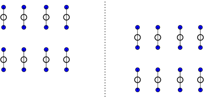
Figure 2: Sketch of the two mean-field ground states occurring for $g>0$ and $t>0$. The blue dots represent the lattice sites. The open circles appear on bonds on which the two Majorana modes combine to form Dirac fermions, which are unoccupied (lowering the energy for nanvanishing $t$). In addition, there are two equivalent states with Dirac fermions occurring on horizontal bonds.

Alternatively, this pairing could occur on sites $(m,2n-1)$ and $(m,2n)$. This is reminiscent of the broken translational symmetry that was found to occur in the 1D model [Rahmani et al., 2015a, b]. This phase can be seen to preserve translation in the horizontal direction, time reversal and parity.

As for the diagonal decoupling (104), the two terms have a different structure, and all parameters $A,B,C$, and $D$ could be potentially nonzero. All these parameters correspond to the uniform and staggered parts of interaction-induced diagonal hopping.

To compare these candidate ground states and estimate the phase diagram, we introduce order parameters into the Hamiltonian. For the case of the vertical order parameter, we first rewrite $H_{int}$ as:

$$H_{int} = -g\sum_{m,n}[i\gamma_{m,n}\gamma_{m,n+1}-A-B(-1)^{n}]$$ (108)

$$\cdot [i\gamma_{m+1,n}\gamma_{m+1,n+1}-A-B(-1)^{n}]$$

$$-2g\sum_{m,n}[A+B(-1)^{n}]i\gamma_{m,n}\gamma_{m,n+1}$$

$$+ g2WL[A^{2}+B^{2}].$$

Notice that the alternating term $2AB(-1)^{n}$ in $[A+B(-1)^{n}]^{2}$ vanishes upon summation over $n$ and does not enter the expression above. We then make the mean-field approximation of ignoring fluctuations, dropping the first term. The parameters $A$ and $B$ are then determined by minimizing the ground state energy of the resulting noninteracting Hamiltonian. Separating the constant proportional to $g(A^{2}+B^{2})$, the rest of the Hamiltonian can be easily diagonalized by modifying the $\gamma^{e\dagger}_{\vec{k}}\gamma^{o}_{\vec{k}}$ term in Eq. (18) and we obtain

$$H^{v}=2i\sum_{k_{x}>0}\gamma^{e\dagger}_{\vec{k}}\gamma^{o}_{\vec{k}}[(t-2gA-2gB)-(t-2gA+2gB)e^{-2ik_{y}}].$$ (109)

The energy levels of Eq. (19) are thus modified to:

$$E_{\pm}\to\pm\sqrt{(4t\sin k_{x})^{2}+[(4t-8gA)\sin k_{y}]^{2}+(8gB\cos k_{y})^{2}}.$$ (110)

Using $\sum_{\vec{k}}\to 2LW\int{d^{2}k\over(2\pi)^{2}}$, the ground-state energy density then becomes

$${E_{0}\over 2WL}\to g(A^{2}+B^{2})+{1\over(2\pi)^{2}}\int_{0}^{\pi}dk_{x}\int_{-\pi/2}^{\pi/2}dk_{y}E_{-}(\vec{k}),$$ (111)

with $E_{-}(\vec{k})$ defined in Eq. (110). Since there is a term linear in $A$ inside the square root in $E_{-}(\vec{k})$, $A$ becomes nonzero for any $g>0$. To first order in $g$, setting $B=0$, we obtain the following ground-state energy per unit area (dropping a constant term):

$${\cal E}\equiv{E_{0}\over 2WL}\approx gA^{2}+{2gA\over\pi^{2}}\int d^{2}k{\sin^{2}k_{y}\over\sqrt{\sin^{2}k_{x}+\sin^{2}k_{y}}}.$$ (112)

Minimizing the energy density $\cal E$, we see that, as $g\to 0^{+}$,

$$A\to-{1\over\pi^{2}}\int d^{2}k{\sin^{2}k_{y}\over\sqrt{\sin^{2}k_{x}+\sin^{2}k_{y}}}.$$ (113)

There is a first-order phase transition into the phase with broken rotational symmetry, but unbroken translational symmetry, at $g=0$.

We then numerically minimize the above energy density over both $A$ and $B$. The results are shown in Fig. (3). The $B$ order parameter remains zero until a second-order phase transition, where it becomes nonzero, at $g\approx 0.9$ for $t_{2}=0$. The presence of diagonal hopping $t_{2}\neq 0$ adds another term, $(8t_{2}\cos k_{x}\cos k_{y})^{2}$ [see Eq. (21)], under the square root in the dispersion relation $E_{\pm}$. Again, the energy can be directly minimized over $A$ and $B$. We find a very similar behavior, as shown, e.g., for $t_{2}=0.5$ in Fig. (3). Indeed, there is a critical point at which $B$ becomes nonzero. As shown in Sec. (VI), in the large $g$ phase the emergent $U(1)$ symmetry is spontaneously broken. While this symmetry breaking transition occurs for both $t_{2}$ zero and nonzero, the universality class of the phase transition is quite different in the two cases, as also discussed in Sec. (VI).

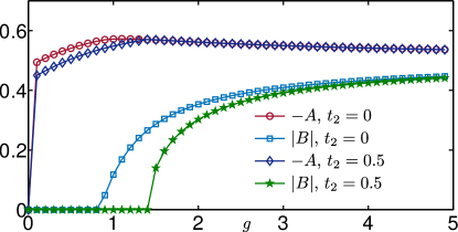
Figure 3: The values of $A$ and $B$ that minimize the energy density (111) ($t_{2}=0$), as a function of $g$. In addition to a first-order transition at $g=0^{+}$, we find a critical point near $g\approx 0.9$. For a finite $t_{2}=0.5$, we also find a critical point and a phase transition to an emergent superfluid phase $|B|>0$. However, this transition is in a different universality class than the $t_{2}=0$ case as the normal phase is gapped (gapless) for $t_{2}\neq 0$ ($t_{2}=0$).

To further analyze the second-order phase transition above for $t_{2}=0$, we set $B=0$ and find $A_{c}(g)$, the value of $A$, which minimizes the energy when $B=0$, as a function of $g$. To determine when a vanishing $B$ stops minimizing the energy, we then compute the derivative of the ground-state energy per unit length, ${\cal F}(g)\equiv{\partial\over\partial B^{2}}{\cal E}(A_{c}(g),B)\Big{|}_{B=0}$ as follows:

$${\cal F}(g)=g-{2g^{2}\over\pi^{2}}\int d^{2}k{\cos^{2}k_{y}\over\sqrt{[1-2gA_{c}(g)]^{2}\sin^{2}k_{y}+\sin^{2}k_{x}}}$$ (114)

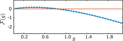
Figure 4: ${\cal F}(g)$, Eq. (114), as a function of $g$. The critical point corresponds to ${\cal F}(g)=0$.

The dependence of ${\cal F}(g)$ on $g$ is shown in Fig. (4). The critical value of $g$, for which $B=0$ is no longer a mean-field solution is given by ${\cal F}(g_{c})=0$, where this derivative changes sign from positive to negative. We find

$$g_{c}\approx 0.852851,\quad A_{c}(g_{c})=-0.566753.$$ (115)

We can further compute ${\cal F}(A_{c}(g_{c}),B)$ at $g=g_{c}$ for small $B$. The results are shown in Fig. (5), indicating a linear dependence on $B$ for small $B$. As discussed in Sec. VI, this linear term is determined by the low energy physics and can be obtained from the field theory approximation.

Finally, if $t_{2}$ is added to the gapless ($B=0$) mean-field Hamiltonian, we have checked that the Chern number remains the same ($\mathcal{C}=-\mathrm{sgn}\;(t_{2}/t)$), given that $A<t/2g$. Therefore for $0<g<g_{c4}$ the gapless line remains the transition between Chern number $1$ and $-1$ states in the mean-field description. Nonzero $B$ gives a gapped phase at zero $t_{2}$, with Chern number $0$.

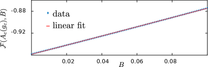
Figure 5: ${\cal F}(A_{c}(g_{c}),B)$ for small $B$.

V.2.2 Diagonal order

We now consider the diagonal order. We follow the same mean-field procedure, rewriting $H_{int}$ in terms of the 4 order parameters introduced in Eq. (102) and ignoring fluctuations, as above. The resulting addition to the noninteracting Hamiltonian is:

$$H^{d}(A,B,C,D) = g\sum_{m,n}[-iO_{m,n}(\gamma_{m,n+1}\gamma_{m+1,n}$$ (116)

$$+ \gamma_{m,n}\gamma_{m+1,n+1})+O^{2}_{m,n}].$$

The constant term now gives

$$g\sum_{m,n}O_{m,n}^{2}=2WLg(A^{2}+B^{2}+C^{2}+D^{2}),$$ (117)

as all terms with an alternating factor vanish upon summation. The rest of the Hamiltonian can be similarly diagonalized although the dispersion relation is lengthy and not very illuminating. Computing the total energy density and minimizing it over the four variables $A,B,C$, and $D$, we find numerically that the minimum energy occurs at $A=B=C=D=0$ for positive $g$. As an example, we plot the energy density as a function of $D$ for $A=B=C=0$ for various values of $g>0$, and observe that a nonzero $D$ only increases the energy, as shown in Fig. (6).

Indeed, from the low-energy field theory (see Sec. VI for details), we expect our mean-field ansatz to potentially only contain a nonvanishing $D$ term in this case:

$$\langle i\gamma_{m,n}\gamma_{m+1,n+1}\rangle=\langle i\gamma_{m,n+1}\gamma_{m+1,n}\rangle=D(-1)^{m+n},$$ (118)

We sketch this state in Fig. (7), for one sign of $D$. This state breaks translation symmetry in the $x$ direction and parity symmetry while preserving translation symmetry in the $y$ direction, time reversal, and $\pi/2$ rotation symmetry. It does not have an interpretation in terms of Majorana fermions pairing to form Dirac fermions. We can show analytically that for $g>0$, $D=0$ at the minimum energy and the vertical decoupling, which is symmetry related to horizontal decoupling, is energetically favorable.

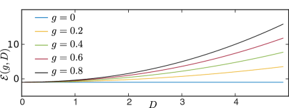
Figure 6: The energy density (123) for $A=B=C=0$ as a function of $D$ for various values of $g$. The minimum energy always corresponds to $D=0$.

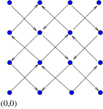
Figure 7: Sketch of the mean-field ground state arising from diagonal factorization of the interaction term for $g>0$, for only $D\neq 0$. An arrow pointing along a diagonal from site $\vec{r}_{1}$ to site $\vec{r}_{2}$ indicates that $i\langle\gamma_{\vec{r}_{1}}\gamma_{\vec{r}_{2}}\rangle>0$.

As before, we obtain the mean-field Hamiltonian by inserting Eq. (118) into the expression for $H^{d}_{int}$. In momentum space, the Hamiltonian becomes

$$H^{d}_{int}\approx 8igD\sum_{\vec{k}}\gamma^{e}_{-\vec{k}+\pi\hat{x}}\gamma^{o}_{\vec{k}}e^{-ik_{y}}\cos k_{x}\cos k_{y}+2LWg{D^{2}}.$$ (119)

It is now convenient to make the replacement $\gamma_{\vec{k}}\to\gamma_{-\vec{k}}^{\dagger}$ for $k_{y}<0$. The Hamiltonian then becomes

$$H=2WLg{D^{2}}+\sum_{k_{x},k_{y}>0}\left(\gamma^{e\dagger}_{\vec{k}},\gamma^{e\dagger}_{\vec{k}-\pi\hat{x}},\gamma^{o\dagger}_{\vec{k}},\gamma^{o\dagger}_{\vec{k}-\pi\hat{x}}\right){\mathscr{H}}\left(\begin{array}[]{c}\gamma^{e}_{\vec{k}}\\ \gamma^{e}_{\vec{k}-\pi\hat{x}}\\ \gamma^{o}_{\vec{k}}\\ \gamma^{o}_{\vec{k}-\pi\hat{x}}\end{array}\right).$$ (120)

where the matrix $\mathscr{H}$ is

$${\mathscr{H}}=\left(\begin{array}[]{cccc}-4t\sin k_{x}&0&-4te^{-ik_{y}}\sin k_{y}&-8igDe^{-ik_{y}}\cos k_{x}\cos k_{y}\\ 0&4t\sin k_{x}&8igDe^{-ik_{y}}\cos k_{x}\cos k_{y}&-4te^{-ik_{y}}\sin k_{y}\\ -4te^{ik_{y}}\sin k_{y}&-8igDe^{ik_{y}}\cos k_{x}\cos k_{y}&-4t\sin k_{x}&0\\ 8igDe^{ik_{y}}\cos k_{x}\cos k_{y}&-4te^{ik_{y}}\sin k_{y}&0&4t\sin k_{x}\end{array}\right),$$ (121)

with the four eigenvalues

$$E^{\pm}_{1} = \pm 4t\sqrt{\sin^{2}k_{x}+\sin^{2}k_{y}}+8gD\cos k_{x}\cos k_{y},$$

$$E^{\pm}_{2} = \pm 4t\sqrt{\sin^{2}k_{x}+\sin^{2}k_{y}}-8gD\cos k_{x}\cos k_{y}.$$ (122)

This gives the ground-state energy density:

$${\cal E}(g,D)={gD^{2}}-{t\over\pi^{2}}\int_{0}^{\pi}dk_{x}\int_{0}^{\pi/2}dk_{y}\left[|\sqrt{\sin^{2}k_{x}+\sin^{2}k_{y}}+2{g\over t}D\cos k_{x}\cos k_{y}|+|\sqrt{\sin^{2}k_{x}+\sin^{2}k_{y}}-2{g\over t}D\cos k_{x}\cos k_{y}|\right].$$ (123)

Dropping a constant, the integral can be seen to be cubic (linear) in $|D|$ for small (large) $|D|$. This can be seen by noting that $|a+b|+|a-b|=2|a|$ for $|a|>|b|$. Therefore, for large $D$, the term in the integral dominates and we get a linear dependence. For small $D$, we can get a $D$-dependent contribution only from a small region in momentum space $\sqrt{\sin^{2}k_{x}+\sin^{2}k_{y}}\approx|\vec{k}|<2gD/t$, leading to a cubic dependence on $D$. Therefore, unsurprisingly, as shown in Fig. (6), the minimum always occurs at $D=0$. Thus the first mean-field state, with order parameter given in Eq. (105), always has lower energy for $g>0$.

V.3 $g<0$

For negative $g$, $H_{int}$ as written in Eq. (101) suggests the following order parameters:

$$\langle i\gamma_{m,n+1}\gamma_{m+1,n+1}\rangle=\langle i\gamma_{m,n}\gamma_{m+1,n}\rangle,$$

$$\langle i\gamma_{m+1,n}\gamma_{m+1,n+1}\rangle=-\langle i\gamma_{m,n}\gamma_{m,n+1}\rangle,$$ (124)

$$\langle i\gamma_{m,n}\gamma_{m+1,n+1}\rangle=-\langle i\gamma_{m,n+1}\gamma_{m+1,n}\rangle.$$ (125)

Again, vertical and horizontal decouplings are related by $\pi/2$ spatial rotation symmetry so we just consider the case of vertical order, and compare it with the diagonal decoupling.

V.3.1 Vertical order

For a $2\times 2$ unit cell, Eq. (124) now corresponds to

$$\langle i\gamma_{m,n}\gamma_{m,n+1}\rangle=C(-1)^{m}+D(-1)^{m+n},$$ (126)

which breaks translational symmetry (in both $x$ and $y$ directions) as well as rotational symmetry, while preserving parity and time reversal. The $D$ term preserves only translational symmetry on diagonals: $\gamma_{m,n}\to\gamma_{m+1,n+1}$ while the $C$ term preserves translation symmetry in the $y$-direction. The $C$ term simply increases or decreases the vertical hopping on alternating columns, while the $D$ term can create a dimerization pattern with stronger bonds forming Dirac fermions as illustrated in Fig. (8). This is analogous to the effect of the $B$ term in the $g>0$ case.

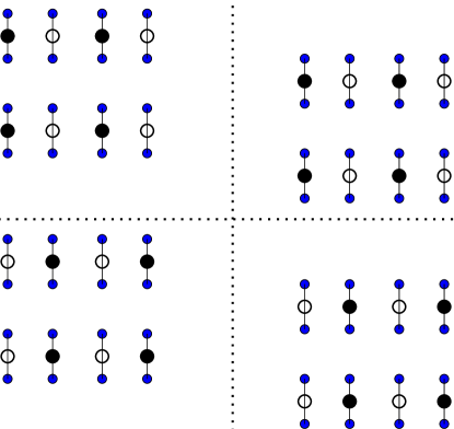
Figure 8: Sketch of four mean field ground states occurring for $g<0$. The blue dots represent lattice sites. The large circles appear on bonds on which the two Majorana modes combine to form Dirac fermions, with filled or empty circles corresponding to the Dirac level being occupied or empty. In addition, there are four equivalent ground states with Dirac fermions occurring on horizontal bonds.

The mean-field interaction Hamiltonian corresponding to Eq. (126) can be written as

$$\begin{split}H^{v}_{int}=2gi\sum_{m,n}&(-1)^{m}\gamma^{e}_{m,2n}[(D+C)\gamma^{o}_{m,2n}+(D-C)\gamma^{o}_{m,2n-2}]\\ &-2LWd(C^{2}+D^{2}).\end{split}$$ (127)

Upon Fourier transformation, the Hamiltonian becomes

$$H^{v}=-2WLg(C^{2}+D^{2})+\sum_{k_{x},k_{y}>0}\left(\gamma^{e\dagger}_{\vec{k}},\gamma^{e\dagger}_{\vec{k}-\pi\hat{x}},\gamma^{o\dagger}_{\vec{k}},\gamma^{o\dagger}_{\vec{k}-\pi\hat{x}}\right){\mathscr{H}}\left(\begin{array}[]{c}\gamma^{e}_{\vec{k}}\\ \gamma^{e}_{\vec{k}-\pi\hat{x}}\\ \gamma^{o}_{\vec{k}}\\ \gamma^{o}_{\vec{k}-\pi\hat{x}}\end{array}\right),$$ (128)

where the matrix $\mathscr{H}$ is now

$$\mathscr{H}=8g\left(\begin{array}[]{cccc}-{t\over 2g}\sin k_{x}&0&-{t\over 2g}e^{-ik_{y}}\sin k_{y}&e^{-ik_{y}}[iD\cos k_{y}+C\sin k_{y}]\\ 0&{t\over 2g}\sin k_{x}&e^{-ik_{y}}[iA\cos k_{y}+B\sin k_{y}]&-{t\over 2g}e^{-ik_{y}}\sin k_{y}\\ -{t\over 2g}e^{ik_{y}}\sin k_{y}&e^{ik_{y}}[-iD\cos k_{y}+C\sin k_{y}]&-{t\over 2g}\sin k_{x}&0\\ e^{ik_{y}}[-iD\cos k_{y}+C\sin k_{y}]&-{t\over 2g}e^{ik_{y}}\sin k_{y}&0&{t\over 2g}\sin k_{x}\end{array}\right).$$ (129)

This gives energy eigenvalues $\pm E_{1,2}$ with

$$E_{1,2}=4\sqrt{(t\sin k_{x})^{2}+(t\sin k_{y})^{2}+(2Dg\cos k_{y})^{2}+(2Cg\sin k_{y})^{2}\pm 4t\sqrt{(\sin k_{x})^{2}(D\cos k_{y})^{2}+(\sin^{2}k_{x}+\sin^{2}k_{y})(C\sin k_{y})^{2}}}.$$ (130)

The ground-state energy density (in the thermodynamic limit) is then given by

$${\cal E}=-g(C^{2}+D^{2})-{1\over(2\pi)^{2}}\int_{0}^{\pi}dk_{x}\int_{0}^{\pi/2}dk_{y}\sum_{i=1}^{2}E_{i}(\vec{k}).$$ (131)

Minimizing the energy density above as a function of $C$ and $D$ gives two first-order phase transitions, when considering the vertical decoupling (we need to compare the energy of these phases with states having diagonal order). Upon increasing $-g$, we first have a phase transition to a state with nonvanishing $D$, which breaks the translation symmetry in the $y$ direction. Diagonal translation is still a symmetry in this phase. Increasing $-g$ further causes a phase transition to a phase with both $C$ and $D$ nonzero, which breaks the translation symmetry in the diagonal direction. In addition to the sudden jump in the order parameters [seen in Fig. (9)], the first-order nature of the phase transitions is confirmed by studying how the energy minima appear. As an example, we plot in Fig. (10), the energy density as a function of $D$ for $C=0$ for several values of $g$. The energy of a local minimum at finite $D$ decreases upon increasing $-g$ and crosses the energy for $D=C=0$ at the first-order phase transition. These phases were obtained by assuming a vertical mean-field decoupling. They may, however, be less favorable than the phases obtained by assuming diagonal decoupling. We will compare the energies after studying the diagonal decoupling case.

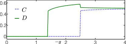
Figure 9: The mean-field parameters minimizing the energy density for the vertical decoupling case with $g<0$. There appears to be two mean-filed transitions; first to a solution with only nonvanishing $D$ and then to a state with both $D$ and $C$ nonzero.

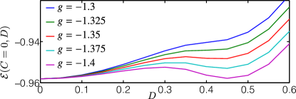
Figure 10: The energy density for various values of $g$ and $C=0$ as a function of $D$, supporting a first-order mean-filed transition.

V.3.2 Diagonal Order

A priori, the diagonal decoupling can have all four terms in Eq. (102), while satisfying the relationship (125). We have computed the general dispersion relation for the diagonal decoupling, and minimized the corresponding ground-state energy over these four parameters. We found that the minimum occurs at $A=C=D=0$ for all value of $g$, while there is a phase transition at strong enough interaction, at which only $B$ becomes nonzero. The results of this numerical minimization are shown in Fig. (11).

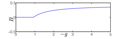
Figure 11: The value of $B$ that minimizes the energy density for the case of diagonal decoupling with $g<0$, indicating a second-order mean-field transition. The minimization yields $A=C=D=0$ for all $g$.

As discussed in the next section, this is indeed expected from the low energy field theory. To simplify the analytical discussion, we thus study the lattice model for the following diagonal candidate mean-field ground states:

$$\langle i\gamma_{m,n}\gamma_{m+1,n+1}\rangle=\langle i\gamma_{m+1,n}\gamma_{m,n+1}\rangle=B(-1)^{n},$$ (132)

which is illustrated in Fig. (12). As seen in Fig. (12), the diagonal order of Eq. (132) simply corresponds to a nonzero diagonal hopping $t_{2}$ [see Eq. (3)]. This order parameter breaks time reversal and parity symmetry while preserving the other symmetries.

The mean-field interaction Hamiltonian can then be written as

$$H^{d}_{int}\approx(igB/8)\sum_{m,ns,s^{\prime}}\gamma_{m,2n}\gamma_{m+s,2n+s^{\prime}}-2gWLB^{2}/64,$$ (133)

where $s$ and $s^{\prime}$ are summed over $\pm 1$. The dispersion relationship then becomes

$$E_{\pm}=\pm 4\sqrt{(t\sin k_{x})^{2}+(t\sin k_{y})^{2}+(2gB\cos k_{x}\cos k_{y})^{2}}.$$ (134)

In terms of the above relationship [Eq. (134)], the ground-state energy per unit area is given by

$${\cal\epsilon}\approx-{gB^{2}}-{1\over(2\pi)^{2}}\int_{0}^{\pi}dk_{x}\int_{-\pi/2}^{\pi/2}dk_{y}E_{+}(\vec{k}).$$ (135)

Treating $gB$ as a small parameter and Taylor expanding, we see that the transition to $B\neq 0$ occurs at

$${1\over g_{c}}\approx-{2\over\pi^{2}t}\int d^{2}k{(\cos k_{x}\cos k_{y})^{2}\over\sqrt{(\sin k_{x})^{2}+(\sin k_{y})^{2}}}.$$ (136)

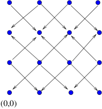
Figure 12: Diagonal ground state for $g<0$. An arrow pointing along a diagonal from site $\vec{r}_{1}$ to site $\vec{r}_{2}$ indicates that $i\langle\gamma_{\vec{r}_{1}}\gamma_{\vec{r}_{2}}\rangle>0$.

Comparing Figs. (9) and (11), we observe that the phase transition in the diagonal case Fig. (11) occurs at a smaller value of $|g|\approx 0.9$ than the transition in the vertical case Fig. (9). However, the energies of the vertical mean-field states are lower than the energy of the diagonal state. We thus find 3 phase transitions at $g<0$. For $-0.9<g<0$, all order parameters vanish and the system is in the gapless phase. For $-1.4<g<-0.9$, diagonal order occurs. For $g<-1.4$ vertical order occurs, with only $A$ nonzero for $-2.4<g<-1.4$ and both $A$ and $B$ nonzero for $g<-2.4$.

Topological analysis of the phases for $g>-0.9$ is analogous to the $g=0$ case. (The mean-field Hamiltonian is not modified). In particular, adding small $t_{2}$ to the gapless phase $-0.9<g<0$ makes it gapped and having Chern number $\mathcal{C}=-\mathrm{sgn}\;(t_{2}/t)$.

VI Field theory approach to interacting model: nature of the phase transitions

The gapless phases for $g_{c3}<g<g_{c4}$ have a low energy field theory description with emergent Lorentz and U(1) symmetries. The transitions out of these phases are both expected to be second order and therefore in the same universality classes as critical points in corresponding Lorentz invariant field theories. By contrast, the transitions at $g_{c2}$ and $g_{c1}$ separate gapped phases and appear to be first order. Therefore, the emergent symmetries and field theory description do not apply. In this section, we analyze the transitions at $g_{c4}$ and $g_{c3}$ using known results on Lorentz invariant field theories. The broken symmetry phases for $g<g_{c2}$ can also be understood from a field theory perspective, which we provide here. However, this field theory perspective is only expected to be of relevance if a continuous transition occurs, which does not seem to be the case. We also analyze, from a field theory perspective, the candidate diagonal broken symmetry state for $g>0$, although it did not occur in the mean-field theory analysis of the previous section.

VI.1 Second-order transitions

For $0<g<g_{c4}$, the mean-field approach of the previous section predicted broken rotational symmetry, with the hopping parameter effectively stronger in the $y$ (or $x$) direction. In the field theory we may simply rescale the $y$-coordinate by a factor of $(1-gA/t)$ to recover full Lorentz invariance. We note that such rescaled rotational invariance is quite common in critical phenomena; it occurs, for example in the two-dimensional classical Ising model at the critical temperature with different couplings in $x$ and $y$ directions.

The prediction of a transition at $g=0$ from a phase with unbroken symmetry at $g<0$ into a phase with effectively stronger hopping in the vertical (or horizontal) direction at $g>0$ is somewhat surprising, given that the interactions are irrelevant. However, since this transition is predicted to be first order, the scaling dimension of the interaction term does not play a role, so this appears possible.

The interaction term in the field theory approximation can be written in two ways:

$${\cal H}_{int}=-64g\psi^{\dagger}_{1}\psi^{\dagger}_{2}\psi_{2}\psi_{1}=32g(\bar{\psi}\psi)^{2}.$$ (137)

For $g>0$ this can be exactly rewritten in terms of a complex scalar field $\phi$ and for $g<0$ in terms of a real scalar field $\sigma$:

$${\cal H}_{int} \to m^{2}|\phi|^{2}+8m\sqrt{g}(\psi^{\dagger}_{1}\psi^{\dagger}_{2}\phi+{\rm H.c.})\ \ (g>0)$$ (138)

$$\to {m^{2}\over 2}\sigma^{2}+8m\sqrt{-g}\bar{\psi}\psi\sigma\ \ (g<0),$$

through a Hubbard-Stratonovich transformation. This is related to the mean-field factorization used in Sec. (V). We can promote the fields $\phi$ and $\sigma$ to relativistic massive fields, with real-time Lagrangians:

$${\cal L} = \bar{\psi}i\gamma^{\mu}\partial_{\mu}\psi+|\partial_{\mu}\phi|^{2}-m^{2}|\phi|^{2}+g_{1}(\psi^{\dagger}_{1}\psi^{\dagger}_{2}\phi+h.c.)$$ (139)

$$- g_{2}|\phi|^{4},\ \ (g>0)$$

$$= \bar{\psi}i\gamma^{\mu}\partial_{\mu}\psi+{1\over 2}(\partial_{\mu}\sigma)^{2}-{m^{2}\over 2}\sigma^{2}+g_{1}\bar{\psi}\psi\sigma-2g_{2}\sigma^{4}.$$

$$\ \ (g<0).$$

Here

$$64g = {g_{1}^{2}\over m^{2}},(g>0)$$ (140)

$$= -{g_{1}^{2}\over m^{2}},(g<0).$$

We have set the velocities to 1 for both fermion and boson fields. As long as $m^{2}$ is positive and large enough we get the correct low energy theory. Note that reducting $m^{2}$ for fixed $g_{1}$ corresponds to increasing $|g|$. We can think of this transition as being driven by reducing $m^{2}$ and letting it change sign. We expect the transitions in this fermion-boson models to be in the same universality classes as the transitions in our pure fermion model. The first Lagrangian in Eq. (139) is the one studied in Refs. [Thomas, 2005; Lee, 2007; Zerf et al., 2016; Fei et al., 2016]. It is expected to have a transition into a superfluid phase. This transition is believed to be SUSY. Both $\phi$ and $\psi$ are massless at the critical point, forming a supermultiplet. The second Lagrangian in Eq. (139) is discussed in Ref. [Fei et al., 2016]. These authors refer to it as the Gross-Neveu-Yukawa model. It also has a transition to a broken symmetry phase as we reduce $m^{2}$ and take it negative. In this case the broken symmetry is just $Z_{2}$, $\sigma\to-\sigma$, $\bar{\psi}\psi\to-\bar{\psi}\psi$. They study the critical exponents at this transition using $\epsilon$-expansion and other techniques. It is not the same as the ordinary Ising transition, which occurs when $g_{1}=0$, due to the presence of the massless fermion field. On the other hand, the transition is not SUSY.

Now we demonstrate the equivalence of these transitions with the ones in the lattice model at $g_{c4}$ and $g_{c3}$. The order parameter for the transition at $g_{c4}$ is

$$\langle i\gamma_{m,n}\gamma_{m,n+1}\rangle=B(-1)^{n}$$ (141)

or, equivalently,

$$\langle i\gamma^{e}_{2n,m}\gamma^{o}_{2n,m}\rangle=\langle i\gamma^{e}_{2n,m}\gamma^{o}_{2n-2,m}\rangle=B$$ (142)

for real $B$ with two different states depending on the sign of $B$. This implies, in the low energy limit,

$$8i\langle\chi^{e+}\chi^{o+}+\chi^{e-}\chi^{o-}\rangle=B$$ (143)

The other two ground states, related by a $\pi/2$ rotation, have

$$i\langle\gamma_{m,n}\gamma_{m+1,n}\rangle=B(-1)^{m+n}$$ (144)

or, equivalently,

$$i\langle\gamma^{e}_{m,2n}\gamma^{e}_{m+1,2n}\rangle=-i\langle\gamma^{o}_{m,2n}\gamma^{o}_{m+1,2n}\rangle=(-1)^{m}B,$$ (145)

which, using Eq. (29), implies

$$16i\langle\chi^{e+}\chi^{e-}\rangle=-16i\langle\chi^{o+}\chi^{o-}\rangle=B.$$ (146)

Note that the Dirac ferimions, defined in Eq. (48), obey

$$\psi_{1}\psi_{2}=(\chi^{e+}\chi^{o+}+\chi^{e-}\chi^{o-})+i(\chi^{e+}\chi^{e-}-\chi^{o+}\chi^{o-}).$$ (147)

Thus, vertical order and horizontal order imply respectively

$$\langle\psi_{1}\psi_{2}\rangle = -iB/8\ \ (\hbox{vertical})$$ (148)

$$= B/8\ \ (\hbox{horizontal}).$$

Recall that the low energy field theory has an emergent $U(1)$ symmetry, corresponding to conservation of Dirac fermion number. The broken symmetry states correspond to spontaneous breaking of this emergent $U(1)$ symmetry. More general ground states would have an arbitrary phase for $\langle\psi_{1}\psi_{2}\rangle$, corresponding to a linear combination of the vertical and horizontal order.

$$E\approx\sqrt{(v\vec{k})^{2}+(8gB)^{2}}$$ (149)

after rescaling the $y$-coordinate. The mean-field transition can also be obtained in the field theory and is again predicted to be second order. The second order nature of the transition, in mean-field theory, is a result of a cubic term in $|B|$ in the Taylor expansion of the ground-state energy, of Eq. (111), which results from the small $k$ region. This cubic term can be obtained in the relativistic approximation using

$${E_{0}/2WL}\approx gB^{2}-{1\over 8\pi^{2}}\int_{k<\Lambda}d^{2}k\sqrt{(vk)^{2}+(8gB)^{2}}.$$ (150)

At small $B$ this gives a universal cubic term $(1/6\pi)|8gB|^{3}$, independent of the cut-off $\Lambda$. The terms in the effective Hamiltonian which break the $U(1)$ (and Lorentz) symmetry are of dimension 6 or higher, more irrelevant than the relativistic interaction term. It is therefore plausible that they remain irrelevant at the critical point. A novel feature of our model is that the boson, and hence the supersymmetry, results from a bosonic bound state of the fermions. This is very reminiscent of the supersymmetric phase transition discovered in the one-dimensional version of this model [Rahmani et al., 2015a, b]. (A field theory discussion of purely fermionic models appears in Ref. [Fei et al., 2016].) Of course, the other novel feature, not occurring in 1D and rather unique to this model, is that the $U(1)$ symmetry, which is spontaneously generated is an emergent symmetry.

Now we consider the transition at $g_{c3}$, the first transition, as $g$ is decreased from $0$, which is into the diagonal phase. Equation (132) implies:

$$8i\langle\chi^{e+}\chi^{o+}-\chi^{e-}\chi^{o+}\rangle=B.$$ (151)

In terms of the Dirac fermions defined in Eq. (48) this becomes:

$$4\bar{\psi}\psi=-B.$$ (152)

This corresponds to spontaneous generation of a mass term for the relativistic fermions, spontaneously breaking time reversal and parity. The dispersion relation of Eq. (134) in the low energy approximation is

$$E_{\pm}=\pm\sqrt{(vk)^{2}+(2gB)^{2}},$$ (153)

corresponding to a mass term. Again the transition is second order due to a term cubic in $|B|$ in the mean-field ground-state energy.

VI.2 Other order parameters

The diagonal order parameter for $g>0$, which apparently does not become nonzero, corresponds, from Eq. (118), to

$$i\langle\gamma^{e}_{m,2n}\gamma^{o}_{m+1,2n}\rangle=A(-1)^{m}.$$ (154)

In the field theory, this corresponds to

$$8i\langle\chi^{e-}\chi^{o+}-\chi^{e+}\chi^{o-}\rangle=A.$$ (155)

Noting that

$$\psi^{\dagger}\psi=2i(\chi^{e-}\chi^{o+}-\chi^{e+}\chi^{o-}),$$ (156)

we see this corresponds to

$$\langle\psi^{\dagger}\psi\rangle=A/4.$$ (157)

This order parameter breaks charge conjugation symmetry and corresponds to adding a chemical potential coupled to the emergent conserved charge. The energy bands of Eq. (122) correspond, at low energies, to energies $vk-8A$ for particles and $vk+8A$ for holes.

Next, we consider the staggered vertical order of Eq. (126), which we found to occur for $g<-1.4$. Setting $D=0$, this corresponds to

$$i\langle\gamma^{e}_{m,2n}\gamma^{o}_{m,2n}\rangle=i\langle\gamma^{e}_{m,2n}\gamma^{o}_{m,2n-2}\rangle=C(-1)^{m}.$$ (158)

In the continuum limit this implies

$$8i\langle\chi^{e+}\chi^{o-}+\chi^{e-}\chi^{o-}\rangle=C.$$ (159)

In terms of the Dirac fermions of Eq. (48), this becomes:

$$\langle\bar{\psi}\gamma^{1}\psi\rangle=-4C.$$ (160)

There is an equivalent mean-field ground state, rotated by $\pi/2$ (uniform horizontal order), with order parameter

$$i\langle\gamma_{m,n}\gamma_{m+1,n}\rangle=C(-1)^{m}.$$ (161)

This implies

$$16i\langle\chi^{e+}\chi^{e-}\rangle=16i\langle\chi^{o+}\chi^{o-}\rangle=C.$$ (162)

Noting that

$$\bar{\psi}\gamma^{2}\psi=-2i(\chi^{e+}\chi^{e-}+\chi^{o+}\chi^{o-}),$$ (163)

we see that this equivalent state has

$$\langle\bar{\psi}\gamma^{2}\psi\rangle=-4C.$$ (164)

As expected, this is obtained by a $\pi/2$ rotation of the state of Eq. (160). Noting that $\bar{\psi}\vec{\gamma}\psi=\vec{J}$, the current operator, we see that these states have a spontaneously generated current, flowing in the $x$ or $y$ direction. More generally, in the field theory, a linear combination of these states would have the same energy, corresponding to the current flowing in an arbitrary direction in the $x$-$y$ plane. The dispersion relation, for order in the $y$ direction, at small $k$ becomes

$$E=(vk_{x}+8Cg)^{2}+(vk_{y})^{2}.$$ (165)

(Note that in the previous section, $k_{x}$ was restricted to positive values. Interpreting the second solution as corresponding to $k_{x}<0$ we have a fixed sign for $A$.) The corresponding mean-field Hamiltonian density is

$${\cal H}=-gC^{2}+\bar{\psi}[-\gamma^{1}(iv\partial_{1}-8gC)-\gamma^{2}iv\partial_{2}]\psi.$$ (166)

We see that $C$ corresponds to a vector potential in the $x$ direction, which leads to a nonzero current. Based on the mean-field calculations in the previous section, we expect the transition into this phase with a spontaneously generated current to be first order.

VI.3 Including second-neighbor hopping term

As discussed in Sec. (II), the second-neighbor hopping term, $\propto t_{2}$, breaks time reversal symmetry and parity (spatial reflection) symmetry. As shown in Sec. (III), it produces an excitation gap which, as shown in Sec. (IV), corresponds to a mass term in the low energy effective field theory. While time reversal and parity are broken by this mass term, Lorentz invariant, the emergent $U(1)$ symmetry and charge conjugation (produce of parity and time reversal) remain good emergent symmetries.

We still expect the emergent superfluid phase to occur for sufficiently large $g>0$, as shown in Sec. (V); see Fig. (3). However, since the fermion now has a finite mass at the critical point, whereas the Goldstone boson is massless, we expect that this transition will no longer be supersymmetric, but instead fall into the usual (2+1) dimensional $U(1)$ breaking universal class. The first transition transition at negative $g$, at $g_{c3}$, no longer occurs since it corresponds to spontaneous breaking of time reversal and parity which are already explicitly broken by the mass term. On the other hand, the first-order transitions at $g_{c1},g_{c2}<0$ into phases with broken spatial rotation symmetry, corresponding to a current flowing in an arbitrary direction, may still occur.

VII Conclusions

We have studied one of the simplest possible 2D models of interacting Majorana modes, using a combination of mean-field theory and renormalization group methods. We find 6 different phases as the coupling strength is varied over both positive and negative values. In particular there are gapless phases at sufficiently weak coupling with emergent Lorentz invariance and U(1) particle number conservation. These are separated by continuous transitions from an emergent superfluid phase for attractive interactions and from a phase with broken time reversal for repulsive interactions. The superfluid transition is predicted to exhibit supersymmetry. The model does not appear to be amenable to Monte Carlo methods since the Majorana modes are not doubled; we intend to present density-matrix renormalization group results on ladders in a later paper.

Appendix A $\pi/2$ rotation symmetry of lattice model

Under the transformation of Eqs. (9) and (10), the nearest-neighbor hopping term transforms as:

$$\sum_{m,n}\gamma_{m,n}[(-1)^{n}\gamma_{m+1,n}+\gamma_{m,n+1}]$$

$$\to\sum_{m,n}\gamma_{-n,m}[\gamma_{-n,m+1}-(-1)^{m}\gamma_{-n-1,m}].$$ (167)

Now redefining the summation variables by $n\to-n$ then $m\leftrightarrow n$, and switching the order of the $\gamma$’s in the second term, we recover the original expression. The interaction term transforms as:

$$\sum_{m,n}\gamma_{m,n+1}\gamma_{m+1,n+1}\gamma_{m+1,n}\gamma_{m,n}$$

$$\to-\sum_{-n-1,m}\gamma_{-n-1,m}\gamma_{-n-1,m+1}\gamma_{-n,m+1}\gamma_{-n,m}.$$ (168)

Redefining the summation variables by $n\to-n$ then $m\leftrightarrow n$, this becomes:

$$-\sum_{m,n}\gamma_{m-1,n}\gamma_{m-1,n+1}\gamma_{m,n+1}\gamma_{m,n}$$

$$=\sum_{m,n}\gamma_{m-1,n+1}\gamma_{m,n+1}\gamma_{m,n}\gamma_{m-1,n}.$$ (169)

Finally, shifting the summation variable, $m\to m+1$ we recover the original term. The second-neighbor hopping term transforms as

$$\sum_{m,n,s,s^{\prime}}\gamma_{m,2n}\gamma_{m+s,2n+s^{\prime}}$$

$$\to\sum_{m,n,s,s^{\prime}}(-1)^{m}\gamma_{-2n,m}\gamma_{-2n-s^{\prime},m+s},$$ (170)

where $s$ and $s^{\prime}$ are summed over $\pm 1$. Redefining summation variables by $n\to-n$ then $m\leftrightarrow n$ together with $s^{\prime}\to-s$, $s\to s^{\prime}$, this becomes

$$\sum_{m,n,s,s^{\prime}}(-1)^{n}\gamma_{2m,n}\gamma_{2m+s,n+s^{\prime}}.$$ (171)

Now treating the even and odd $n$ terms separately, this can be written:

$$\sum_{m,n,s,s^{\prime}}[\gamma_{2m,2n}\gamma_{2m+s,2n+s^{\prime}}-\gamma_{2m,2n+1}\gamma_{2m+s,2n+1+s^{\prime}}].$$ (172)

In the second term we then switch order of the $\gamma$ factors, redefine $2n+1+s^{\prime}\to 2n$ (for each value of $s^{\prime}$) and redefine $2m+s\to 2m+1$ (for each value of $s$). The term then becomes

$$\sum_{m,n,s,s^{\prime}}[\gamma_{2m,2n}\gamma_{2m+s,2n+s^{\prime}}+\gamma_{2m+1,2n}\gamma_{2m+1+s,2n+s^{\prime}}].$$ (173)

Combining the two terms gives the original expression.

Appendix B Normalization in Eq. (29)

Equation (29) implies, for example, that $\chi^{e+}$ contains the Fourier modes of $\chi^{e}$ near $\vec{k}=0$, divided by $2\sqrt{2}$. Thus, also using Eq. (12),

$$\chi^{e+}={1\over 2\sqrt{2}}\sqrt{2\over WL}\sum_{|\vec{k}|<\Lambda}e^{i\vec{k}\cdot\vec{r}}\gamma^{e}_{\vec{k}}.$$ (174)

From Eq. (13), we see that $\Delta k_{x}=2\pi/L$ and $\Delta k_{y}=\pi/W$. Thus

$$\{\chi^{e+}(\vec{r}),\chi^{e+}(\vec{r}^{\prime})\} = {1\over 8}{2\over WL}\sum_{k<\Lambda}e^{i\vec{k}\cdot(\vec{r}-\vec{r}^{\prime})}$$ (175)

$$= {1\over 2}\int_{k<\Lambda}{d^{2}k\over(2\pi)^{2}}e^{i\vec{k}\cdot(\vec{r}-\vec{r}^{\prime})}$$

$$\approx {1\over 2}\delta^{2}(\vec{r}-\vec{r}^{\prime}),$$

showing that $\chi^{e+}$ has the correct normalization. A similar result holds for all 4 fields, $\chi^{e/o\pm}$.

References

- König et al. (2007) M. König, S. Wiedmann, C. Brüne, A. Roth, H. Buhmann, L. W. Molenkamp, X.-L. Qi, and S.-C. Zhang, Science 318, 766 (2007).
- Zhang et al. (2009) H. Zhang, C.-X. Liu, X.-L. Qi, X. Dai, Z. Fang, and S.-C. Zhang, Nature physics 5, 438 (2009).
- Xia et al. (2009) Y. Xia, D. Qian, D. Hsieh, L. Wray, A. Pal, H. Lin, A. Bansil, D. Grauer, Y. Hor, R. Cava, et al., Nature Physics 5, 398 (2009).
- Mourik et al. (2012) V. Mourik, K. Zuo, S. M. Frolov, S. Plissard, E. Bakkers, and L. P. Kouwenhoven, Science 336, 1003 (2012).
- Alicea (2012) J. Alicea, Reports on Progress in Physics 75, 076501 (2012).
- Beenakker (2013) C. Beenakker, Annu. Rev. Condens. Matter Phys. 4, 113 (2013).
- Nayak et al. (2008) C. Nayak, S. H. Simon, A. Stern, M. Freedman, and S. D. Sarma, Reviews of Modern Physics 80, 1083 (2008).
- Hyart et al. (2013) T. Hyart, B. Van Heck, I. Fulga, M. Burrello, A. Akhmerov, and C. Beenakker, Physical Review B 88, 035121 (2013).
- Aasen et al. (2016) D. Aasen, M. Hell, R. V. Mishmash, A. Higginbotham, J. Danon, M. Leijnse, T. S. Jespersen, J. A. Folk, C. M. Marcus, K. Flensberg, et al., Physical Review X 6, 031016 (2016).
- Karzig et al. (2016) T. Karzig, C. Knapp, R. Lutchyn, P. Bonderson, M. Hastings, C. Nayak, J. Alicea, K. Flensberg, S. Plugge, Y. Oreg, et al., arXiv preprint arXiv:1610.05289 (2016).
- Kitaev (2001) A. Y. Kitaev, Physics-Uspekhi 44, 131 (2001).
- Fu and Kane (2008) L. Fu and C. L. Kane, Physical review letters 100, 096407 (2008).
- Lutchyn et al. (2010) R. M. Lutchyn, J. D. Sau, and S. D. Sarma, Physical review letters 105, 077001 (2010).
- Oreg et al. (2010) Y. Oreg, G. Refael, and F. von Oppen, Physical review letters 105, 177002 (2010).
- Albrecht et al. (2016) S. M. Albrecht, A. Higginbotham, M. Madsen, F. Kuemmeth, T. S. Jespersen, J. Nygård, P. Krogstrup, and C. Marcus, Nature 531, 206 (2016).
- Zhou et al. (2013) J. Zhou, Y.-J. Wu, R.-W. Li, J. He, and S.-P. Kou, EPL (Europhysics Letters) 102, 47005 (2013).
- Biswas (2013) R. R. Biswas, Physical review letters 111, 136401 (2013).
- Chiu et al. (2015) C.-K. Chiu, D. Pikulin, and M. Franz, Physical Review B 91, 165402 (2015).
- Liu and Franz (2015) T. Liu and M. Franz, Phys. Rev. B 92, 134519 (2015).
- Pikulin et al. (2015) D. Pikulin, C.-K. Chiu, X. Zhu, and M. Franz, Physical Review B 92, 075438 (2015).
- Hermanns and Trebst (2014) M. Hermanns and S. Trebst, Phys. Rev. B 89, 235102 (2014).
- Rahmani et al. (2015a) A. Rahmani, X. Zhu, M. Franz, and I. Affleck, Physical review letters 115, 166401 (2015a).
- Rahmani et al. (2015b) A. Rahmani, X. Zhu, M. Franz, and I. Affleck, Phys. Rev. B 92, 235123 (2015b).
- Milsted et al. (2015) A. Milsted, L. Seabra, I. Fulga, C. Beenakker, and E. Cobanera, Physical Review B 92, 085139 (2015).
- Witczak-Krempa and Maciejko (2016) W. Witczak-Krempa and J. Maciejko, Physical review letters 116, 100402 (2016).
- Ware et al. (2016) B. Ware, J. H. Son, M. Cheng, R. V. Mishmash, J. Alicea, and B. Bauer, Physical Review B 94, 115127 (2016).
- Gangadharaiah et al. (2011) S. Gangadharaiah, B. Braunecker, P. Simon, and D. Loss, Physical review letters 107, 036801 (2011).
- Lobos et al. (2012) A. Lobos, R. Lutchyn, and S. Das Sarma, Physical review letters 109, 146403 (2012).
- Grosfeld and Stern (2006) E. Grosfeld and A. Stern, Physical Review B 73, 201303 (2006).
- Park et al. (2015) Y. Park, S. Jung, and J. Maciejko, Phys. Rev. B 91, 054507 (2015).
- Zhu and Franz (2016) X. Zhu and M. Franz, Phys. Rev. B 93, 195118 (2016).
- Hayata and Yamamoto (2017) T. Hayata and A. Yamamoto, arxiv:1705.00135 (2017).
- Li et al. (2015) Z.-X. Li, Y.-F. Jiang, and H. Yao, Phys. Rev. B 91, 241117 (2015).
- Thomas (2005) S. Thomas, seminar at KITP (2005).
- Lee (2007) S.-S. Lee, Phys. Rev. B 76, 075103 (2007).
- Ponte and Lee (2014) P. Ponte and S.-S. Lee, New Journal of Physics 16, 013044 (2014).
- Jian et al. (2015) S.-K. Jian, Y.-F. Jiang, and H. Yao, Phys. Rev. Lett. 114, 237001 (2015).
- Zerf et al. (2016) N. Zerf, C.-H. Lin, and J. Maciejko, Phys. Rev. B 94, 205106 (2016).
- Grover et al. (2014) T. Grover, D. Sheng, and A. Vishwanath, Science 344, 280 (2014).
- Wen (2004) X.-G. Wen, Quantum field theory of many-body systems: from the origin of sound to an origin of light and electrons (Oxford University Press on Demand, 2004).
- Nielsen and Ninomiya (1981) H. B. Nielsen and M. Ninomiya, Nucl. Phys. B 185, 20 (1981).
- O’Brien et al. (2017) T. E. O’Brien, C. W. J. Beenakker, and I. Adagideli, Phys. Rev. Lett. 118, 207701 (2017).
- Fei et al. (2016) L. Fei, S. Giombi, I. Klebanov, and G. Tarnopolsky, Prog. Theor. Exp. Phys. 2016, 12C105 (2016).