Fractional Bhatnagar-Gross-Krook kinetic equation

Abstract

The linear Boltzmann equation approach is generalized to describe fractional superdiffusive transport of the Lévy walk type in external force fields. The time distribution between scattering events is assumed to have a finite mean value and infinite variance. It is completely characterized by the two scattering rates, one fractional and a normal one, which defines also the mean scattering rate. We formulate a general fractional linear Boltzmann equation approach and exemplify it with a particularly simple case of the Bohm and Gross scattering integral leading to a fractional generalization of the Bhatnagar, Gross and Krook kinetic equation. Here, at each scattering event the particle velocity is completely randomized and takes a value from equilibrium Maxwell distribution at a given fixed temperature. We show that the retardation effects are indispensable even in the limit of infinite mean scattering rate and argue that this novel fractional kinetic equation provides a viable alternative to the fractional Kramers-Fokker-Planck (KFP) equation by Barkai and Silbey and its generalization by Friedrich et al. based on the picture of divergent mean time between scattering events. The case of divergent mean time is also discussed at length and compared with the earlier results obtained within the fractional KFP.

1 Introduction

Linear Boltzmann equation Hoare provides a versatile tool to describe kinetics of the test or impurity particles in a background gas of abundant particles serving as a thermal bath. Consider test particles of mass $M$ characterized by the distribution function $f(x,v,t)$, where $x$ is the particle position, $v=\dot{x}$ is its velocity and $t$ is time. The particles are subjected to an external force $F(x,v,t)$ and obey the Newtonian equations of motion $M\ddot{x}=F(x,v,t)$, where $x$, $v$, and $F$ are generally vectors with three Cartesian components. In this paper, we are dealing for simplicity with a one-dimensional scalar form. However, the major results can easily be generalized to higher dimensions. From time to time the impurity particles are scattering with the background gas particles and their velocities are changed at each scattering event. Any kinetic equation can be written in the form $df(x,v,t)/dt={\rm St}[f(x,v,t)]$, where $d/dt$ is a full derivative and ${\rm St}[f(x,v,t)]$ is a scattering integral (Stoßintegral), or collision term. In the absence of scattering events, $df(x,v,t)/dt=0$ expresses just the Liouville theorem of classical mechanics, or conservation of the number of particles in an elementary phase volume $dxdp$, $p=Mv$. This number changes due to scattering events yielding income and outcome of the particles in any given phase volume. At the equilibrium, the both processes are balanced, and hence ${\rm St}[f_{\rm eq}(x,v)]=0$, where $f_{\rm eq}(x,v)$ is equilibrium distribution. Generally, ${\rm St}[f(x,v,t)]$ is a nonlinear function of $f(x,v,t)$, like in the classical nonlinear Boltzmann equation, which takes binary collisions between the particles of one-component gas into account. However, in the case of a two-component gas, when the gas of the test particles is very dilute, the scattering events among the test particles can be simply neglected because they are very rare, and this leads to a linear Boltzmann equation (LBE),

$$\frac{\partial f(x,v,t)}{\partial t} +v\frac{\partial f(x,v,t)}{\partial x}+\frac{F(x,v,t)}{M}\frac{\partial f(x,v,t)}{\partial v}$$ (1)

$$= -r(v)f(x,v,t)+\int dv^{\prime}w(v\leftarrow v^{\prime})f(x,v^{\prime},t),$$

where $w(v^{\prime}\leftarrow v)$ is the rate of transitions in the velocity space, and $r(v)=\int dv^{\prime}w(v^{\prime}\leftarrow v)$ is a total rate. The first line presents the full derivative of the distribution function, and the second line is a particular linear form of the scattering integral. It says that the scattering in the velocity subspace is described by a standard master equation. In writing this equation one implicitly assumes that the time between the scattering events is exponentially distributed. This is the reason why the scattering integral is local in time, and underlying dynamics is Markovian. The standard Kramers-Fokker-Planck equation presents a limiting case of LBE, where a diffusional approximation is done in the scattering integral Hoare ; Risken , which we write in the following generic form consistent with thermodynamics Klimontovich

$${\rm St}[f(x,v,t)] = \frac{\partial}{\partial v}\left(D(v)e^{-\beta Mv^{2}/2}\frac{\partial}{\partial v}e^{\beta Mv^{2}/2}f(x,v,t)\right)$$ (2)

$$= \frac{\partial}{\partial v}\left[\gamma(v)\left(v+v_{T}^{2}\frac{\partial}{\partial v}\right)f(x,v,t)\right],$$

where $\beta=1/(k_{B}T)$ is inverse temperature, $D(v)=v_{T}^{2}\gamma(v)$, $\eta(v)=M\gamma(v)$ is a nonlinear, generally velocity-dependent friction coefficient, and $v_{T}=\sqrt{k_{B}T/M}$ is thermal velocity. This form emerges with the help of the Kramers-Moyal expansion vanKampen in the master equation. For example, in the particular case of $\gamma(v)=\gamma=const$ one can use a modified Rayleigh model of the scattering kernel

$$w(v\leftarrow v^{\prime})=\frac{1}{4}\gamma\kappa\sqrt{\frac{\kappa}{2\pi v_{T}^{2}}}e^{-\frac{\kappa(v-v^{\prime}+(v^{\prime}+v)/\kappa)^{2}}{8v_{T}^{2}}}\;,$$ (3)

where $\kappa=M/m$ is the ratio of the masses of the test and background particles. This is a modification of the standard Rayleigh kernel, see Eq. (3.4) in Hoare or Eq. (4.14) in vanKampen , where differently from the standard model we assume that the frequency of collisions does not depend on the relative velocity of the test particles and the particles of the thermal bath. For this reason, the prefactor in (3) does not contain the difference of velocities $|v-v^{\prime}|$. In this modified Rayleigh model, the total collision rate is $r(v)=r=(1/2)\gamma\kappa^{2}/(\kappa+1)$. Eq. (2) is obtained exactly with $\gamma(v)=\gamma=const$ from the scattering integral in Eq. (1) upon using the Kramers-Moyal expansion and taking the limit $\kappa\to\infty$ . Notice that then also $r\to\infty$. This corresponds physically to the case where the scattering events occur very often, and the background gas of light particles is dense and fluid-like (heavy Brownian particles in a fluid). The first line in (2) makes it immediately clear that this equation is compatible with the thermal equilibrium, where $f_{\rm eq}(x,v)=p_{x}(x)f_{M}(v)$ and

$$f_{M}(v)=\exp[-v^{2}/(2v_{T}^{2})]/\sqrt{2\pi v_{T}^{2}}$$

is the equilibrium Maxwellian velocity distribution.

Another important instance of the LBE equation is provided by a Bohm and Gross form of the scattering integral Bohm . It can be obtained from the modified Rayleigh model (3) in the case $\kappa=1$, i.e. the test particles and the particles of the thermal bath have equal masses. In this case,

$$w(v\leftarrow v^{\prime})=rf_{M}(v),$$

with the collision rate $r=\gamma/4$. The physical meaning of this choice is as follows. Time-intervals between scattering events are exponentially distributed with the mean time $\langle\tau\rangle=1/r$, and after each scattering event the particle’s velocity is fully randomized in the correspondence with its thermally equilibrium distribution $f_{M}(v)$. The scattering integral in this case reads BGR ,

$${\rm St}[f(x,v,t)]=-r\left[f(x,v,t)-f_{M}(v)\int dvf(x,v,t)\right],$$ (4)

and the corresponding kinetic equation is known as Bhatnagar, Gross and Krook (BGK) kinetic equation BGR ; Risken ; Zwanzig . This one is considered typically as a linear approximation to a nonlinear Boltzmann equation, where the distinct background and impurity particles have yet nearly equal masses. In the kinetic equation for the reduced distribution function of velocities, $p(v,t)=\int dxf(x,v,t)$ in the velocity subspace, the scattering term looks especially simple, $-r\left[p(v,t)-f_{M}(v)\right]$, which corresponds to a single relaxation time approximation ($F=0$ here),

$$\partial p(v,t)/\partial t=-r\left[p(v,t)-f_{M}(v)\right].$$

In particular, because of this simplicity, BGK kinetic equation became popular in the literature Zwanzig , especially in the context of lattice Boltzmann models Succi aimed at the lattice simulations of hydrodynamics. In this respect, derivation of the hydrodynamics equations from the BGK kinetic equation is especially simple and insightful Zwanzig , what underlines its general importance and a possibly wide range of applications beyond gaseous systems like plasmas.

It is the main purpose of this paper to generalize this linear Boltzmann equation description towards a fractional Lévy walk kinetics in the velocity space Kenkre73 ; Shlesinger ; Scher ; Bouchaud ; Hughes ; Balescu ; BenAvraham ; Geisel88 ; Zumofen93 ; ZumofenPhysicaD ; West97 ; Barkai96 ; Barkai97 ; BarkaiPRE97 ; Metzler00 , where the times between scattering events are non-exponentially distributed and possess a finite first moment, i.e. the mean time $\langle\tau\rangle$ between the scattering events remains finite Geisel88 ; Zumofen93 ; ZumofenPhysicaD ; West97 ; Barkai97 ; BarkaiPRE97 ; GoychukPRE12 . Moreover, we will pay an essential attention to the limit $\langle\tau\rangle\to 0$. In this respect, our theory differs much from the fractional Kramers-Fokker-Planck (KFP) equation by Barkai and Silbey Barkai00 , and its further correction and generalization by Friedrich et al. FriedrichPRL06 ; FriedrichPRE06 based on the picture of infinite $\langle\tau\rangle\to\infty$, even if it is related closely in several aspects to the theory developed in FriedrichPRL06 ; FriedrichPRE06 .

2 Theory

We start from considering the scattering process as a continuous time random walk (CTRW) Kenkre73 ; Shlesinger ; Scher ; Bouchaud ; Hughes ; Balescu ; BenAvraham in the velocity space or as a Lèvy walk Geisel88 ; Bouchaud ; Zumofen93 ; ZumofenPhysicaD ; Hughes ; Balescu ; BenAvraham ; Barkai96 ; West97 ; Barkai97 ; BarkaiPRE97 ; Metzler00 . The particles fly with a constant velocity $v$ between any two subsequent scattering events and such events change their velocity from $v$ to $v^{\prime}$ with a transition probability density $W(v^{\prime}\leftarrow v)$. We will consider the case, where the mean time between the scattering events exists and it defines the mean scattering rate $r=1/\langle\tau\rangle$. Then, $w(v^{\prime}\leftarrow v)=rW(v^{\prime}\leftarrow v)$. All scattering events are assumed to be mutually independent.

2.1 Lévy walk in the velocity space

In the velocity space, such a decoupled semi-Markovian Lévy walk is fully characterized by the residence time distribution or RTD $\psi(\tau)$ of the time-intervals between two scattering events and the transition probability density $W(v^{\prime}\leftarrow v)$. We consider first the dynamics of the velocity distribution $p(v,t)=\int dxf(x,v,t)$. It is governed by a generalized master equation (GME), which is well-known by analogy with such a decoupled CTRW in the coordinate space. This GME reads Kenkre73

$$\frac{\partial p(v,t)}{\partial t}=-r(v)\int_{0}^{t}dt^{\prime}K(t-t^{\prime})p(v,t^{\prime})$$ (5)

$$+\int_{0}^{t}dt^{\prime}K(t-t^{\prime})\int dv^{\prime}w(v\leftarrow v^{\prime})p(v^{\prime},t^{\prime})\;,$$

with a memory kernel $K(t)$ whose Laplace-transform is $\tilde{K}(s)=(1/r)s\tilde{\psi}(s)/[1-\tilde{\psi}(s)]=(1/r)\tilde{\psi}(s)/\tilde{\Phi}(s)$, in terms of the Laplace-transformed RTD $\tilde{\psi}(s)$. It can be expressed also through the survival probability $\Phi(\tau)=\int_{\tau}^{\infty}\psi(t)dt$, which is the probability to do not have any scattering event within a time interval of length $\tau$. If this survival probability is exponential, $\Phi(\tau)=\exp(-rt)$, then $K(t)=\delta(t)$ and Eq. (5) is the standard LBE for the force-free case in the velocity space.

We consider a generalization of this LBE, where the RTD between two scattering presents a sum,
$\psi(\tau)=\sum_{j=0}^{N}\psi_{j}(\tau)$ over $N+1$ independent scattering channels, and the corresponding Laplace-transforms read GoychukPRE12

$$\tilde{\psi}_{j}(s)=r_{\alpha_{j}}s^{1-\alpha_{j}}\tilde{\Phi}(s),\;$$ (6)

where

$$\tilde{\Phi}(s)=\frac{1}{s+\sum_{j=0}^{N}r_{\alpha_{j}}s^{1-\alpha_{j}}}\;$$ (7)

with $0<\alpha_{j}\leq 1$ is the Laplace-transformed survival probability $\Phi(t)$, and $r_{\alpha_{j}}$ are the fractional scattering rates. We demand that one of them is normal, $\alpha_{0}=1$, and at least one of them is anomalous. The normal rate $r_{\alpha_{0}}=1/\langle\tau\rangle=r$ defines the mean scattering rate, The variance of $\tau$ in this model is infinite due to anomalous scattering channels. This distribution has been derived in Ref. GoychukPRE12 in assumption that each of the scattering channels taken separately is characterized by a Mittag-Leffler distribution $\psi_{j}^{(sep)}(\tau)=-(d/d\tau)E_{\alpha_{j}}(-r_{\alpha_{j}}\tau^{\alpha_{j}})$, where $E_{\alpha}(z)=\sum_{n=0}^{\infty}z^{n}/\Gamma(n\alpha+1)$ is the Mittag-Leffler function, and one of the independent channels is taken randomly at each scattering event, i.e. they are acting intermittently and in parallel. Here, $\Gamma(x)$ is a standard special $\Gamma$-function. The averaged number of the scattering events in this model grows as $\langle n(t)\rangle=\sum_{j}r_{\alpha_{j}}t^{\alpha_{j}}/\Gamma(1+\alpha_{j})$. For simplicity, we will restrict our attention to the model with one normal and one fractional scattering rates. Then, $\langle n(t)\rangle=rt+r_{\alpha}t^{\alpha}/\Gamma(1+\alpha)$, exactly. Notice, that with respect to the averaged number of the scattering events, an anomalous scattering channel contributes really a little for sufficiently large $t$. However, its role in the kinetics is really profound!

We wish to find the diffusional spread of the variance of the particles position $\langle x^{2}(t)\rangle$ assuming that at the initial time $t_{0}=0$ they all were localized at the coordinate origin, $x(0)=0$. For this, we need to know the velocity autocorrelation function (ACF) of two arguments $K_{v}(t,t^{\prime})=\langle v(t^{\prime})v(t^{\prime\prime})\rangle$. Indeed, by using $x(t)=\int_{0}^{t}v(t^{\prime})dt$, we have $\langle x^{2}(t)\rangle=\int_{0}^{t}dt^{\prime}\int_{0}^{t}dt^{\prime\prime}\langle v(t^{\prime})v(t^{\prime\prime})\rangle$. To find such a nonstationary, or aging velocity ACF is not a trivial task Cox ; Godreche ; Allegrini05 ; Margolin05 ; Froemberg13 . For example, in the case of two-state velocity fluctuations it was solved in Ref. Froemberg13 . A further simplification is possible for the case of a stationary ACF $K_{v}^{(\rm st)}(|t-t^{\prime}|)$, which depends only on the difference of two time arguments. Then,

$$\langle x^{2}(t)\rangle =2\int_{0}^{t}dt^{\prime}\int_{0}^{t^{\prime}}dt^{\prime\prime}K_{v}^{(\rm st)}(|t^{\prime}-t^{\prime\prime}|)$$

$$=2\int_{0}^{t}(t-t^{\prime})K_{v}^{(\rm st)}(t^{\prime})dt^{\prime}.$$

In this important case, the Laplace-transform of $\langle x^{2}(t)\rangle$ reads $\widetilde{\langle x^{2}(s)\rangle}=2\tilde{K}_{v}^{(\rm st)}(s)/s^{2}$, where $\tilde{K}_{v}^{(\rm st)}(s)$ is the Laplace-transform of $K_{v}^{(\rm st)}(\tau)$.

It must be stressed, however, that the GME (5) corresponds to a CTRW, which starts at the time $t_{0}=0$ from a scattering event Tunaley . As a matter of fact, if to calculate the ACF $K_{v}(t,0)$ for $t\geq 0$ using this master equation and an initially equilibrium $p(v,0)=f_{M}(v)$, we obtain not the stationary ACF $K_{v}^{(\rm st)}(t)$, but just a non-stationary velocity ACF $K_{v}(t_{\rm ag}+t,t_{\rm ag})$ taken at zero age time $t_{\rm ag}=0$ Cox . This one simply cannot be used in Eq. (2.1). To use it therein, would be a profound mistake. To find $K_{v}(t_{\rm ag}+t,t_{\rm ag})$, one needs to consider an aging CTRW, where the survival probability of the first scattering time interval $\Phi^{(0)}(t|t_{\rm ag})$ is different and age-dependent. It can be found from the following reasoning. Assume that scattering events started at the time $-t_{\rm ag}$ in the past relative to the starting point $t_{0}=0$ of observations. Then, if we observe our system from $t_{0}=0$ to $t$, the corresponding survival probability to do not have a scattering event is $\Phi(t+t_{\rm ag})$. However, $n$ undetected scattering events might already took place until any “unseen” time point $-y$ within the time interval $[-t_{\rm ag},0]$ in the past and then no events occurred until $t$. Integrating over $y$ and summing over all possible $n$ yields the following exact result Cox ; Godreche ; Allegrini05

$$\Phi^{(0)}(t|t_{\rm ag})= \Phi(t+t_{\rm ag})$$ (9)

$$+ \sum_{n=1}^{\infty}\int_{0}^{t_{a}}\psi_{n}(t_{a}-y)\Phi(t+y)dy,$$

where $\psi_{n}(t)$ is the probability density to have $n$ scattering events. It is the $n$-time convolution of the density $\psi(\tau)$, $\tilde{\psi}_{n}(s)=[\tilde{\psi}(s)]^{n}$ in the Laplace space. From (9), one can easily find the double Laplace transform $\tilde{\Phi}^{(0)}(s|u)$ of $\Phi^{(0)}(t|t_{\rm ag})$, where $s$ is the Laplace-transform variable, which is conjugated to $t$, and $u$ to $t_{\rm ag}$. Some algebra yields simple result GoychukCTP14

$$\tilde{\Phi}^{(0)}(s|u)=\frac{1}{u(s-u)}\left(1-\frac{\tilde{\Phi}(s)}{\tilde{\Phi}(u)}\right)\;.$$ (10)

The Laplace-transform of the fully aged or equilibrium $\Phi^{(0)}(t)=\lim_{t_{\rm ag}\to\infty}\Phi^{(0)}(t|t_{\rm ag})$, the first-time stationary survival probability, can be obtained now as $\tilde{\Phi}^{(0)}(s)=\lim_{u\to 0}u\tilde{\Phi}^{(0)}(s|u)$. For $\tilde{\Phi}(0)=\langle\tau\rangle\neq\infty$ this yields the well-known result $\tilde{\Phi}^{(0)}(s)=(1-\tilde{\Phi}(s)/\langle\tau\rangle)/s$ Cox ; Tunaley ; GoychukPRL03 ; GoychukPRE04 ; GoychukCTP14 . The corresponding first-interval RTD is $\psi^{(0)}(t)=\Phi(t)/\langle\tau\rangle$, which is also well-known. Using this $\psi^{(0)}(t)$ one can derive another GME, which corresponds to a time-homogeneous initial preparations of the scattering process. This was done in the Appendix of Ref. GoychukPRE04 , in a different context. Applying that GME to our scattering process we obtain,

$$\frac{\partial p(v,t)}{\partial t}=-r(v)\int_{0}^{t}dt^{\prime}K(t-t^{\prime})[p(v,t^{\prime})-p(v,0)]$$

$$+\int_{0}^{t}dt^{\prime}K(t-t^{\prime})\int dv^{\prime}w(v\leftarrow v^{\prime})[p(v^{\prime},t^{\prime})-p(v^{\prime},0)]\;$$

$$-r(v)p(v,0)+\int dv^{\prime}w(v\leftarrow v^{\prime})p(v^{\prime},0)\;.$$ (11)

This equation corresponds to the following initial preparation. We first trap the particles in a space trap and let them pre-equilibrate with the particles of the thermal bath by multiple collisions before we release them from the trap. The distribution of velocities at $t_{0}=0$ can still be out of equilibrium. This is what van Kampen named as “extraction of a subensemble” vanKampen . We are doing such a procedure for non-Markovian renewal processes with finite $\langle\tau\rangle$. Notice that in the limit $\langle\tau\rangle\to\infty$ such an extraction of subensemble is not possible in principle, because the corresponding random process simply does not have even a wide-sense stationary limit. The process $v(t)$ is still non-stationary for $p(v,0)\neq p_{\rm st}(v)$. However, the memory kernel of transition probabilities depends now merely on the time shift indeed. Very important is that $K_{v}(t,0)$ found with the help of GME (2.1) is indeed the stationary velocity ACF, $K_{v}(t,0)=K_{v}^{(\rm st)}(t)$, $t\geq 0$. Namely, the solution of (2.1) with $p(v,0)=\delta(v-v^{\prime})$ yields the time-shift invariant propagator of velocities $\Pi^{\rm(st)}(v,t|v^{\prime},0)$, and

$$K_{v}^{\rm(st)}(t)=\int\int vv^{\prime}\Pi^{\rm(st)}(v,t|v^{\prime},0)p_{\rm st}(v^{\prime})dvdv^{\prime}\;,$$ (12)

where $p_{\rm st}(v)=\lim_{t\to\infty}p(v,t)$ is the stationary solution.

Next, our fractional BGK master equation is characterized by the RTD having the characteristic function or the Laplace transform

$$\tilde{\psi}(s)=\frac{r+r_{\alpha}s^{1-\alpha}}{s+r+r_{\alpha}s^{1-\alpha}},\;$$ (13)

and by a complete randomization of the velocity at each scattering event in accordance with the Maxwellian distribution of velocities, like in the kinetic model of Refs. Barkai97 ; BarkaiPRE97 . Arguably, this is a simplest fractional generalization of the kinetic BGK model possible. Notice, that $\psi(t)$ has $\psi(t)\propto t^{-3+\alpha}$ long-time asymptotics within this model GoychukPRE12 ; GoychukCTP14 . The Laplace-transform of the survival probability reads $\tilde{\Phi}(s)=1-s\tilde{\psi}(s)$ or

$$\tilde{\Phi}(s)=\frac{1}{s+r+r_{\alpha}s^{1-\alpha}},\;$$ (14)

and the first-time survival probability is

$$\tilde{\Phi}^{(0)}(s)=\frac{1+r_{\alpha}s^{-\alpha}}{s+r+r_{\alpha}s^{1-\alpha}}\;$$ (15)

in the Laplace-domain. Furthermore, the GME (5) yields a time-inhomogeneous fractional BGK kinetic equation in the velocity space GoychukCTP14

$$\frac{\partial p(v,t)}{\partial t}=-\left(r+r_{\alpha}\sideset{{}_{0}}{{}_{t}}{\mathop{\hat{D}}^{1-\alpha}}\right)\left[p(v,t)-f_{M}(v)\right],$$ (16)

where $\sideset{{}_{0}}{{}_{t}}{\mathop{\hat{D}}^{1-\alpha_{j}}}$ is the operator of Riemann-Liouville fractional derivative defined as Metzler00 ; Gorenflo

$$\sideset{{}_{0}}{{}_{t}}{\mathop{\hat{D}}^{\gamma}}f(t):=\frac{1}{\Gamma(1-\gamma)}\frac{\partial}{\partial t}\int_{0}^{t}dt^{\prime}\frac{f(t^{\prime})}{(t-t^{\prime})^{\gamma}}$$ (17)

by its action on a test function $f(t)$, $0<\gamma<1$. This is an example of kinetic equations with fractional derivatives of distributed order distro . Moreover, the GME (2.1) for this model yields

$$\frac{\partial p(v,t)}{\partial t}=-r_{\alpha}\sideset{{}_{0}}{{}_{t}}{\mathop{\hat{D}}^{1-\alpha}}\left[p(v,t)-p(v,0)\right]$$ (18)

$$-r\left[p(v,t)-f_{M}(v)\right]\;.$$

3 Fractional superdiffusion from the velocity space perspective

We proceed further with showing that the considered description in the velocity space does yield fractional superdiffusion in the coordinate space. For this, we calculate $K^{\rm(st)}_{v}(|t-t^{\prime}|)$. Here, we can use the solution of Eq. (18), which is easy to obtain in the Laplace-domain. In the time-domain, it reads

$$p(v,t)=f_{M}(v)+\Phi^{(0)}(t)[p(v,0)-f_{M}(v)]\;,$$ (19)

like in Barkai97 . Hence, the stationary propagator or stationary, time-shift invariant conditional probability of the velocity distribution reads $\Pi^{\rm(st)}(v,t|v^{\prime},0)=f_{M}(v)+\Phi^{(0)}(t)[\delta(v-v^{\prime})-f_{M}(v)]$, and with $p_{\rm st}(v)=f_{M}(v)$ in (12) we obtain

$$K_{v}^{\rm(st)}(|t-t^{\prime}|)=v_{T}^{2}\Phi^{(0)}(|t-t^{\prime}|)\;.$$ (20)

Notice a remarkable simplicity if this result within the studied scattering model: the normalized stationary velocity autocorrelation function just equals to the equilibrium survival probability of the first scattering time intervals. A similar result was obtain within a mathematically related model for dielectric relaxation which describes a stationary generalized Cole-Cole response GoychukCTP14 , and also earlier within a different model with just two-state, $\pm v$, velocity fluctuations Geisel88 ; West97 . By the same token, we find upon the use of Eq. (16), $K_{v}(t,0)=v_{T}^{2}\Phi(t)$. Notice once again that this later $K_{v}(t,0)$ cannot be used to find $\langle x^{2}(t)\rangle$. This is a nonstationary velocity ACF for zero aging time.

3.1 The limit $\langle\tau\rangle\to\infty$ or $r\to 0$

In this limit, which alludes to the fractional KFP equation of Refs. Barkai00 ; FriedrichPRL06 ; FriedrichPRE06 , we obtain from Eq. (15), $\Phi^{(0)}(t)=1$, like in Ref. GoychukCTP14 . Hence, $K_{v}^{\rm(st)}(|t-t^{\prime}|)=v_{T}^{2}$, i.e. it does not decay at all! In accordance with the Slutsky-Khinchine theorem Papoulis , this means that such a stochastic process $v(t)$ is not ergodic. This also implies that $\langle x^{2}(t)\rangle=v_{T}^{2}t^{2}$, i.e. diffusion is asymptotically ballistic, universally for any $0<\alpha<1$. Clearly, this is an asymptotic regime of fully aged $K_{v}(t+t_{\rm ag},t_{\rm ag})$, $t_{\rm ag}\to\infty$. It was not studied in Refs. Barkai00 ; FriedrichPRL06 ; FriedrichPRE06 , where $t_{\rm ag}=0$ in fact. Interestingly, in this latter case we obtain also $K_{v}(t,0)=v_{T}^{2}E_{\alpha}(-r_{\alpha}t^{\alpha})$, i.e. the same result as for a different model in Barkai00 . From it, one cannot, however, conclude anything on the behavior of $\langle x^{2}(t)\rangle$, even for $t_{\rm ag}=0$. The correct asymptotical result in the case $t_{\rm ag}=0$ is $\langle x^{2}(t)\rangle\sim(1-\alpha)v_{T}^{2}t^{2}$, as it will be shown below from a different perspective in agreement with FriedrichPRL06 ; FriedrichPRE06 for the retarded version of the fractional KFP equation. We stress, however, that a finite value of $\langle\tau\rangle$ is a very essential feature of our approach justifying $t_{\rm ag}=\infty$ as a very common experimental condition. Actually, it is hard to imagine how an experimental system of scattering particles can be prepared exactly at $t_{\rm ag}=0$.

3.2 The limit $\langle\tau\rangle\to 0$, $r_{\alpha}\to\infty$, $\langle\tau\rangle r_{\alpha}=const$

Another important limit is $\langle\tau\rangle=1/r\to 0$, $r_{\alpha}\to\infty$, i.e. of very fast scattering events, so that $\tau_{r}=(r_{\alpha}/r)^{1/(1-\alpha)}=const$. In this case, $K_{v}^{\rm(st)}(t)=v_{T}^{2}E_{1-\alpha}[-(t/\tau_{r})^{1-\alpha}]$, which reminds the Barkai and Silbey result Barkai00 for $r\to 0$ and nonstationary $K_{v}(t,0)$. However, our result contains $\alpha$ instead of $1-\alpha$, and also its meaning is very different, in spite of a perplexedly confusing similarity. Furthermore, a similar result, but with $2-\alpha$ instead of $1-\alpha$ and $1<\alpha<2$ was obtained for the stationary velocity ACF within a very different model of super-diffusion based on the fractional Langevin equation with super-Ohmic coupling to a thermal bath of harmonic oscillators MainardiPeroni ; Lutz ; SiegleEPL ; GoychukACP12 . The physics of both models is, however, entirely different. In our case, the corresponding position variance grows as

$$\langle x^{2}(t)\rangle=2(v_{T}t)^{2}E_{1-\alpha,3}[-(t/\tau_{r})^{1-\alpha}],$$ (21)

where $E_{\alpha,b}(z)=\sum_{n=0}^{\infty}z^{n}/\Gamma(\alpha n+b)$ is a generalized Mittag-Leffler function. For $t\ll\tau_{r}$, $\langle x^{2}(t)\rangle\approx(v_{T}t)^{2}$, and diffusion is initially ballistic. This is because $K_{v}^{\rm(st)}(t)\approx v_{T}^{2}$ on this time scale. For $t\gg\tau_{r}$, $K_{v}^{\rm(st)}(t)\propto 1/t^{1-\alpha}$, and $\langle x^{2}(t)\rangle\propto t^{1+\alpha}$, i.e. an asymptotic sub-ballistic superdiffusion regime emerges. Interestingly, it is mostly close to the ballistic diffusion for $\alpha=1-\epsilon$, $\epsilon\to+0$, and not for $\alpha\to 0$, as in Ref. Barkai00 . This is a rather paradoxical and unexpected feature since in this case the anomalous scattering channel is mostly close to the normal one within the model studied.

3.3 General case of $\langle\tau\rangle>\tau_{r}$

The result of previous subsection holds approximately very good for $\langle\tau\rangle\ll\tau_{r}$. For $\langle\tau\rangle\gg\tau_{r}$, $K_{v}^{\rm(st)}(t)$ decays first exponentially, $K_{v}^{\rm(st)}(t)\approx v_{T}^{2}\exp(-t/\langle\tau\rangle)$, and at $t_{c}\sim c\langle\tau\rangle$, where $c$ is a numerical coefficient about $c\sim 10$, a transition occurs to an algebraic tail behavior, $K_{v}^{\rm(st)}(t)\propto 1/t^{1-\alpha}$, see in Fig. 1. Therein, $K_{v}^{\rm(st)}(t)$ is plotted for different values of $\langle\tau\rangle$ in the cases $\alpha=1/2$, where an exact analytical expression can be readily found by the inversion of the Laplace-transform, and $\alpha=0.75$, where we invert the Laplace-transform numerically using the Stehfest-Gaver algorithm Stehfest . The analytical expression for $\alpha=0.5$ reads

$$K_{v}^{\rm(st)}(t)=\frac{v_{T}^{2}}{\sqrt{\tau_{1}}-\sqrt{\tau_{2}}}$$ (22)

$$\times\left[\sqrt{\tau_{1}}E_{1/2}\left(-\sqrt{\frac{t}{\tau_{1}}}\right)-\sqrt{\tau_{2}}E_{1/2}\left(-\sqrt{\frac{t}{\tau_{2}}}\right)\right]\;,$$

where $E_{1/2}(-\sqrt{z})=\exp(z){\rm erfc}(\sqrt{z})$, is the Mittag-Leffler function with index $\alpha=1/2$ and argument $-\sqrt{z}$, and $\tau_{1,2}=\tau_{r}\left(1\pm\sqrt{1-4\langle\tau\rangle/\tau_{r}}\right)^{2}/4$. The stationary ACF has a power law tail, $K_{v}^{\rm(st)}(t)\propto t^{-1+\alpha}$, see in Fig. 1. A similar algebraic tail features also the velocity ACF in simple fluids. It emerges due to the hydrodynamic memory effects yielding $K_{v}^{\rm(st)}(t)\propto t^{-1.5}$ asymptotically Zwanzig ; MainardiPeroni ; GoychukACP12 . However, very different from the hydrodynamic memory case, in our model this algebraic tail is not integrable and it yields asymptotically a superdiffusion, $\langle x^{2}(t)\rangle\propto t^{1+\alpha}$. In this respect, it is also very important to mention that the zero-age $K_{v}(t,0)$ for $\alpha=1/2$ reads

$$K_{v}(t,0)=\frac{v_{T}^{2}}{\sqrt{\tau_{1}}-\sqrt{\tau_{2}}}$$ (23)

$$\times\left[\sqrt{\tau_{1}}E_{1/2}\left(-\sqrt{\frac{t}{\tau_{2}}}\right)-\sqrt{\tau_{2}}E_{1/2}\left(-\sqrt{\frac{t}{\tau_{1}}}\right)\right]\;.$$

Notice a very subtle difference between (23) and (22), which is not easy to spot! A structurally very same equation was obtained for the stationary velocity ACF within the fractional Langevin equation by Mainardi and Peroni MainardiPeroni , wherein $r$ is related to the standard Stokes friction and $r_{1/2}$ to the hydrodynamic memory effects. Asymptotically, $K_{v}(t,0)\propto t^{-3/2}$. For a large $\langle\tau\rangle$, it starts also from an exponential part $K_{v}(t,0)\approx\exp(-t/\langle\tau\rangle)$, like $K_{v}^{\rm(st)}(t)$, cf. in Fig. 2, which ends in the $t^{-3/2}$ tail. For a small $\langle\tau\rangle$, it displays also another intermediate power law $K_{v}(t,0)\propto t^{-1/2}$, like $K_{v}^{\rm(st)}(t)$ asymptotically.

Furthermore, the exact expression for the position variance in the case $\alpha=1/2$ reads

$$\langle x^{2}(t)\rangle=2(v_{T}t)^{2}\frac{1}{\sqrt{\tau_{1}}-\sqrt{\tau_{2}}}$$ (24)

$$\times\left[\sqrt{\tau_{1}}E_{1/2,3}\left(-\sqrt{\frac{t}{\tau_{1}}}\right)-\sqrt{\tau_{2}}E_{1/2,3}\left(-\sqrt{\frac{t}{\tau_{2}}}\right)\right]\;,$$

where

$$E_{1/2,3}(-\sqrt{z})=z^{-2}\Big{[}-1+\frac{2}{\sqrt{\pi}}z^{1/2}-z+\frac{4}{3\sqrt{\pi}}z^{3/2}$$

$$+E_{1/2}(-\sqrt{z})\Big{]}\;.$$ (25)

This expression shares the following general features for other values of $\alpha$. For $\langle\tau\rangle\gg\tau_{r}$, diffusion is initially ballistic for $0<t\ll\langle\tau\rangle$. Then, it becomes transiently normal for $\langle\tau\rangle<t<c\langle\tau\rangle$. Finally, after slowing down it again accelerates and becomes sub-ballistic superdiffusion with

$$\langle x^{2}(t)\rangle\sim 2(v_{T}\tau_{r})^{2}(t/\tau_{r})^{1+\alpha}/\Gamma(2+\alpha)$$ (26)

for $t\gg c\langle\tau\rangle$, see in Fig. 3. Notice that this is the same asymptotics independently of $\langle\tau\rangle$ as one produced by the result in Eq. (21). One can clearly see that with growing $\langle\tau\rangle$, the initial regime of ballistic diffusion extends gradually to infinity while $\langle\tau\rangle\to\infty$, independently of $\alpha$.

Furthermore, if to use mistakingly $K_{v}(t,0)$ instead of $K_{v}^{\rm(st)}(t)$ in Eq. (2.1), we obtain

$$\langle x^{2}(t)\rangle=2(v_{T}t)^{2}\frac{1}{\sqrt{\tau_{1}}-\sqrt{\tau_{2}}}$$ (27)

$$\times\left[\sqrt{\tau_{1}}E_{1/2,3}\left(-\sqrt{\frac{t}{\tau_{2}}}\right)-\sqrt{\tau_{2}}E_{1/2,3}\left(-\sqrt{\frac{t}{\tau_{1}}}\right)\right]\;.$$

The formal difference with (24) is not easy to detect. However, the diffusive behavior is very different, see in Fig. 4 and compare with Fig. 3, (a). First of all, asymptotically this is a normal diffusion, although the initial regime of ballistic diffusion, which is also universal, gradually extends to infinity with growing $\langle\tau\rangle$. Intermittently, it can be sub-ballistic superdiffusion with $\langle x^{2}(t)\rangle\propto t^{3/2}$, as for $\langle\tau\rangle=0.001$ in Fig. 4 (it looks like initial regime therein because the truly initial ballistic regime is simply not depicted for this value of parameter).

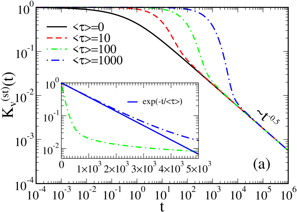
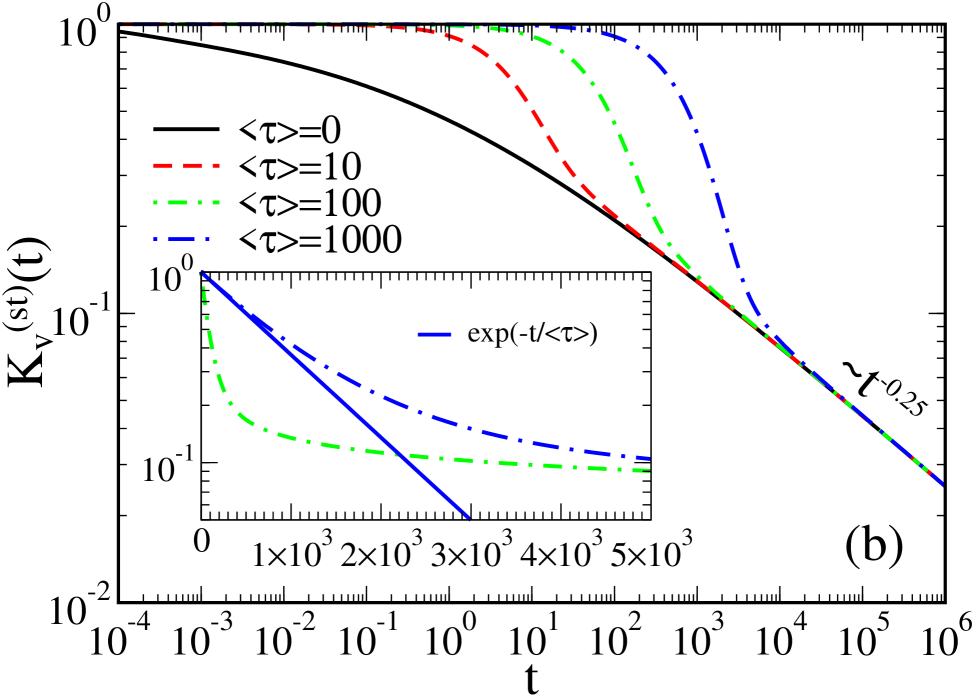
Figure 1: (Color online) Normalized stationary velocity autocorrelation function as function of time (in units of $\tau_{r}$) for (a) $\alpha=0.5$, and (b) $\alpha=0.75$, as well as different values of $\langle\tau\rangle$ shown in the plot. The results in (a) are exact analytical results, whereas the results in (b) are obtained by a numerically precise inversion of the corresponding Laplace transform using the Stehfest-Gaver algorithm. The inset shows a part of the same plot on semi-logarithmic scale to reveal an initially exponential decay indicated by a solid line in the inset for $\langle\tau\rangle=1000$.

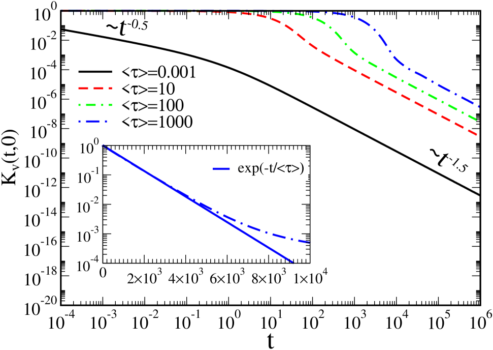
Figure 2: (Color online) Normalized velocity autocorrelation function $K_{v}(t,0)$ as function of time (in units of $\tau_{r}$) for $\alpha=0.5$, and different values of $\langle\tau\rangle$ shown in the plot. The inset shows a part of the same plot on semi-logarithmic scale to reveal an initially exponential decay indicated by a solid line in the inset for $\langle\tau\rangle=1000$.

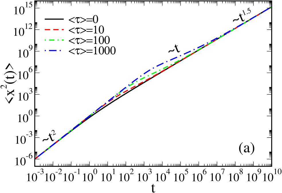
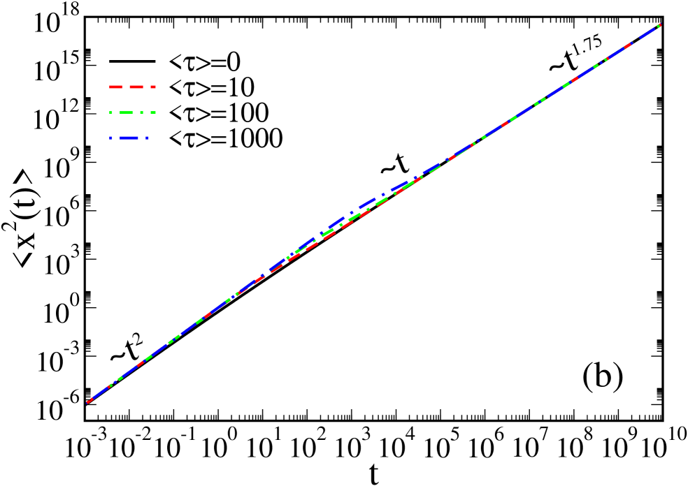
Figure 3: (Color online) Variance of particles position (in units of $(v_{T}\tau_{r})^{2}$) as function of time (in units of $\tau_{r}$) for (a) $\alpha=0.5$, and (b) $\alpha=0.75$, as well as different values of $\langle\tau\rangle$ shown in the plot. The results in (a) are exact analytical results, while the results in (b) are obtained by a numerically precise inversion of the corresponding Laplace transform.

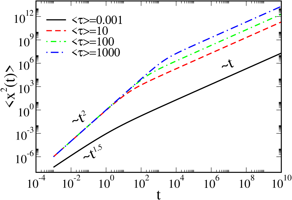
Figure 4: (Color online) Variance of particles position (in units of $(v_{T}\tau_{r})^{2}$) as function of time (in units of $\tau_{r}$) for $\alpha=0.5$ and different values of $\langle\tau\rangle$ if to substitute ad hoc $K_{v}^{\rm(st)}(t)$ with $K_{v}(t,0)$ in Eq. (2.1).

4 Fractional BGK equations in the phase space

We proceed further with a generalization of the above description from the velocity subspace to the whole phase space because we wish to have a kinetic description valid in arbitrary force fields $F\neq 0$. It turns out to be a very nontrivial task. First, following Friedrich et al. FriedrichPRL06 ; FriedrichPRE06 one must take the retardation effects into account. For the case $F=0$, this can be done exactly. Namely, from Eq. (5) we obtain the corresponding scattering integral

$${\rm St}[f(x,v,t)]=-r(v)\int_{0}^{t}dt^{\prime}K(t-t^{\prime})f(X(t,t^{\prime}),v,t^{\prime})$$

$$+\int_{0}^{t}dt^{\prime}K(t-t^{\prime})\int dv^{\prime}w(v\leftarrow v^{\prime})f(X^{\prime}(t,t^{\prime}),v^{\prime},t^{\prime})$$

in the phase space, where $X(t,t^{\prime})$ and $X^{\prime}(t,t^{\prime})$ in Eq. (4) are the retarded spatial variables reading, $X(t,t^{\prime})=x-v(t-t^{\prime})$ and $X^{\prime}(t,t^{\prime})=x-v^{\prime}(t-t^{\prime})$. Because $F=0$, the velocity remains constant between two scattering events. The physical meaning of these variables and their origin is clear. Because $x(t)=\int_{0}^{t}v(t^{\prime})dt^{\prime}$, both $X(t,t^{\prime})$ and $X^{\prime}(t,t^{\prime})$ are just the values of the coordinate $x$ at the time $t^{\prime}$, i.e. $x(t^{\prime})$, for two different constant values of the velocity variable. This retardation, which results from a rigorous treatment of the scattering process in the phase space FriedrichPRL06 ; FriedrichPRE06 , makes everything rather intricate, especially in the presence of external force fields, when $F\neq 0$. Then, most obviously not only $X(t,t^{\prime})=x-\int_{t^{\prime}}^{t}v(\tau)d\tau$ generally, but also a retardation in the velocity variable should be taken into account. To neglect this latter one is only possible if the acceleration of the particles between two scattering events is negligible. We wish to explore a possibility to avoid such complexities and to disregard the retardation effects whenever it can safely be done. Intuitively, this can only be physically justified if $\langle\tau\rangle$ is finite and a relative change of $f(x,v,t)$ on the spatial scale $x_{T}=v_{T}\langle\tau\rangle$ is completely negligible. At the first look, it seems that using $\langle\tau\rangle$ sufficiently small, this approximation can always be justified, which is definitely not the case of $\langle\tau\rangle=\infty$, like in the case of fractional Kramers-Fokker-Planck equation by Barkai and Silbey. The latter one corresponds to the case, where the only one anomalous scattering channel is present and the scattering integral is taken in the KFP form with a velocity-independent friction coefficient $\eta$, and the retardation effects are completely disregarded. For the considered model of scattering mechanism, a general fractional linear Boltzmann equation (FLBE) with retardation can readily be written

$$\frac{\partial f(x,v,t)}{\partial t}+v\frac{\partial f(x,v,t)}{\partial x}+\frac{F(x,v,t)}{M}\frac{\partial f(x,v,t)}{\partial v}$$

$$= -\left(1+(r_{\alpha}/r)\sideset{{}_{0}}{{}_{t}}{\mathop{\hat{\cal D}}^{1-\alpha_{j}}}\right)\Big{[}r(v)f(x,v,t^{\prime})$$

$$-\int dv^{\prime}w(v\leftarrow v^{\prime})f(x,v^{\prime},t^{\prime})\Big{]},$$

where

$$\sideset{{}_{0}}{{}_{t}}{\mathop{\hat{\cal D}}^{\gamma}}f(x,v,t)=\frac{1}{\Gamma(1-\gamma)}$$

$$\times\left(\frac{\partial}{\partial t}+v\frac{\partial}{\partial x}\right)\int_{0}^{t}dt^{\prime}\frac{f(x-v(t-t^{\prime}),v,t^{\prime})}{(t-t^{\prime})^{\gamma}}\;.$$ (29)

is the operator of substantial fractional derivative, which takes the retardation of the $x$ variable into account FriedrichPRL06 ; FriedrichPRE06 . Here, one implicitly assumes that between two scattering events the particles velocity is not changed in spite of the external force applied. This, of course, can only be done if either $\langle\tau\rangle$ is sufficiently small, or when $F=0$ exactly. Furthermore, a fractional generalization of the BGK kinetic equation or fractional BGK kinetic equation (FBGKE) reads

$$\frac{\partial f(x,v,t)}{\partial t}+v\frac{\partial f(x,v,t)}{\partial x}+\frac{F(x,v,t)}{M}\frac{\partial f(x,v,t)}{\partial v}$$ (30)

$$= -\left(r+r_{\alpha}\sideset{{}_{0}}{{}_{t}}{\mathop{\hat{\cal D}}^{1-\alpha}}\right)\left[f(x,v,t)-f_{M}(v)\int dvf(x,v,t)\right]\;.$$

These kinetic equations correspond, however, to the case when the scattering events started at $t_{0}=0$. What will happen if the scattering events started in the infinite past at the age $-t_{\rm ag}$, $t_{\rm ag}\to\infty$? In this case, we can adopt GME (2.1) for writing the collision term upon taking the retardation effects in the $x$ variable into account in the following manner:

$${\rm St}[f(x,v,t)]=-r(v)\int_{0}^{t}dt^{\prime}K_{\alpha}(t-t^{\prime})$$ (31)

$$\times[f(X(t,t^{\prime}),v,t^{\prime})-f(X(t,0),v,0)]$$

$$+\int_{0}^{t}dt^{\prime}K_{\alpha}(t-t^{\prime})\int dv^{\prime}w(v\leftarrow v^{\prime})$$

$$\times[f(X^{\prime}(t,t^{\prime}),v^{\prime},t^{\prime})-f(X^{\prime}(t,0),v^{\prime},0)]$$

$$-r(v)f(x,v,t)+\int dv^{\prime}w(v\leftarrow v^{\prime})f(x,v^{\prime},t)\;.$$

Here, a singular memory kernel (which is not a function but a distribution) has the Laplace-transform $\tilde{K}_{\alpha}(s)=r_{\alpha}s^{1-\alpha}$.

The corresponding fully-aged version of our fractional BGK equation with retardation reads

$$\frac{\partial f(x,v,t)}{\partial t}+v\frac{\partial f(x,v,t)}{\partial x}+\frac{F(x,v,t)}{M}\frac{\partial f(x,v,t)}{\partial v}$$ (32)

$$= -\Big{(}r+r_{\alpha}\sideset{{}_{0}}{{}_{t}}{\mathop{\hat{\cal D}}^{1-\alpha}}\Big{)}\Big{[}f(x,v,t)-f_{M}(v)\int dvf(x,v,t)\Big{]}$$

$$+\int_{0}^{t}K_{\alpha}(t-t^{\prime})\Big{[}f(x+vt,v,0)$$

$$-f_{M}(v)\int f(x+v^{\prime}t,v^{\prime},0)dv^{\prime}\Big{]}dt^{\prime}\;.$$

Can we disregard the retardation overall and to replace the substantial fractional derivative by the standard one, for example, in the limit $\langle\tau\rangle\to 0$? This is a fundamental question which will be answered below. Fractional kinetic equations (4), (30), and (32) present the central theoretical proposals of this paper.

5 Fractional superdiffusion within FBGKE

The next important task is to establish if we do can neglect the retardation effects in the fractional kinetic equations in the phase space, and when it is possible in principle.

5.1 Standard form of FBGKE with retardation and without

We start from the standard form of the force-free ($F=0$) FBGKE (30), which takes the retardation effects into account. In terms of the double Fourier transform of the distribution function,
$\hat{G}(k,\eta,t)=\int_{-\infty}^{\infty}dx\int_{-\infty}^{\infty}dve^{i(kx+\eta v)}f(x,v,t)$, which is the moment-generating function, this equation can be written as

$$\frac{\partial\hat{G}(k,\eta,t)}{\partial t}-k\hat{G}^{\prime}_{\eta}(k,\eta,t)=-\int_{0}^{t}K(t-t^{\prime})$$

$$\times\Big{[}\hat{G}(k,\eta+k(t-t^{\prime}),t^{\prime})-e^{-(\eta v_{T})^{2}/2}\hat{G}(k,k(t-t^{\prime}),t^{\prime})\Big{]},$$

where $\hat{G}^{\prime}_{\eta}(k,\eta,t)$ denotes a partial derivative with respect to the variable $\eta$, with retardation effects taken into account, and

$$\frac{\partial\hat{G}(k,\eta,t)}{\partial t}-k\hat{G}^{\prime}_{\eta}(k,\eta,t)=-\int_{0}^{t}K(t-t^{\prime})$$ (34)

$$\times\Big{[}\hat{G}(k,\eta,t^{\prime})-e^{-(\eta v_{T})^{2}/2}\hat{G}(k,0,t^{\prime})\Big{]},$$

without. These equations are difficult to solve. However, by setting $k=0$ therein we can readily deduce that the corresponding FBGE in the velocity space reads (16) independently of whether we took the retardation effects into account or not. This is the same feature as with the fractional KFP equation FriedrichPRE06 . Furthermore, the discussed equations can be used to find the equations of motion for the moments of coordinate and velocity by taking a corresponding number of derivatives of $\hat{G}(k,\eta,t)$ with respect to $k$ and $\eta$ at $k=0,\eta=0$. In this way, we obtain from Eq. (5.1):

$$\frac{d}{dt}\langle x^{2}(t)\rangle=2\langle x(t)v(t)\rangle,$$ (37)

$$\frac{d}{dt}\langle x(t)v(t)\rangle=\langle v^{2}(t)\rangle-\int_{0}^{t}K(t-t^{\prime})$$

$$\times\Big{[}\langle x(t^{\prime})v(t^{\prime})\rangle+\langle v^{2}(t^{\prime})\rangle(t-t^{\prime})\Big{]}dt^{\prime},$$

$$\frac{d}{dt}\langle v^{2}(t)\rangle=-\int_{0}^{t}K(t-t^{\prime})\big{[}\langle v^{2}(t^{\prime})\rangle-v_{T}^{2}\big{]}dt^{\prime}\,.$$

If to neglect the retardation effects, Eq. (37) is replaced by

$$\frac{d}{dt}\langle x(t)v(t)\rangle=\langle v^{2}(t)\rangle-\int_{0}^{t}K(t-t^{\prime})\langle x(t^{\prime})v(t^{\prime})dt^{\prime}.$$ (38)

This is the only difference. Solving Eq. (37), we obtain

$$\widetilde{\langle v^{2}(s)\rangle}=\frac{\langle v^{2}(0)\rangle s+v_{T}^{2}\tilde{K}(s)}{s[s+\tilde{K}(s)]},$$ (39)

or $\langle v^{2}(t)\rangle=v_{T}^{2}+\Phi(t)[\langle v^{2}(0)\rangle-v_{T}^{2}]$ in the time domain, which is consistent with the above-given solution for $p(v,t)$ in this case. The latter one has precisely the same relaxation structure. Furthermore, Eq. (37) can be solved by using the convolution theorem and noticing that the Laplace-transform of $K(t)t$ reads $-\tilde{K}^{\prime}(s)$, where $\tilde{K}^{\prime}(s)$ is the derivative over $s$. Finally, with the initial conditions $\langle x^{2}(0)\rangle=0$ and $\langle x(0)v(0)\rangle=0$ we obtain for the Laplace-transformed position variance

$$\widetilde{\langle x^{2}(s)\rangle}=\frac{2[1+\tilde{K}^{\prime}(s)][\langle v^{2}(0)\rangle s+v_{T}^{2}\tilde{K}(s)]}{s^{2}[s+\tilde{K}(s)]^{2}}\;.$$ (40)

Similar expression for a particular case $\langle v^{2}(0)\rangle=0$ has been obtained by Friedrich et al. FriedrichPRE06 for a different model (fractional Kramers-Fokker-Planck equation with retardation effects) in different notations. To compare with the above solutions obtained in the velocity domain, it is useful to take the equilibrium distribution of velocities initially. This yields

$$\widetilde{\langle x^{2}(s)\rangle}=\frac{2v_{T}^{2}[1+\tilde{K}^{\prime}(s)]}{s^{2}[s+\tilde{K}(s)]}\;.$$ (41)

Furthermore, if to neglect the retardation effects the latter equation is modified as

$$\widetilde{\langle x^{2}(s)\rangle}=\frac{2v_{T}^{2}}{s^{2}[s+\tilde{K}(s)]}\;.$$ (42)

It gives precisely the same result in the time domain as if incorrectly use $K_{v}(t,0)$ in Eq. (2.1) instead of $K_{v}^{\rm(st)}(t)$. This is actually very misleading! This masking unfortunate feature reflects profound problems emerging immediately if to neglect the retardation effects. Let us discuss the related subtleties.

5.1.1 Fractional FBGKE with infinite $\langle\tau\rangle$

In this case $r=0$, and Eq. (41) yields

$$\widetilde{\langle x^{2}(s)\rangle}=\frac{2v_{T}^{2}[1+(1-\alpha)r_{\alpha}s^{-\alpha}]}{s^{2}[s+r_{\alpha}s^{1-\alpha}]}\;,$$ (43)

including retardation effects. The corresponding
$\langle x^{2}(t)\rangle=\langle x^{2}_{1}(t)\rangle+\langle x^{2}_{2}(t)\rangle$ consists of two parts. The first corresponds to the neglect of the retardation effects, and this is precisely the result by Barkai and Silbey, $\langle x_{1}^{2}(t)\rangle=2(v_{T}t)^{2}E_{\alpha,3}[-r_{\alpha}t^{\alpha}]$, obtained for a different model. Asymptotically, $\langle x_{1}^{2}(t)\rangle\propto t^{2-\alpha}$. Notice, however, that in the sum the second term, $\langle x_{2}^{2}(t)\rangle\sim v_{T}^{2}(1-\alpha)t^{2}$, dominates asymptotically, which is the result by Friedrich et al. for a different KFP model FriedrichPRE06 . Interestingly, the same asymptotics and a similar subleading term were also obtained by Barkai and Fleurov within a kinetically related model Barkai96 . The same ballistic asymptotics with prefactor $1-\alpha$ was obtained also by Zumofen and Klafter within a different model ZumofenPhysicaD . This result is the correct result for the case of zero age, $t_{\rm ag}=0$. Furthermore, notice the difference of prefactors $1-\alpha$ for $t_{\rm ag}=0$, and just one for $t_{\rm ag}=\infty$, where $K_{v}^{\rm(st)}(t)=v_{T}^{2}=const$.

5.1.2 Fractional FBGKE with finite $\langle\tau\rangle$

In this case,

$$\widetilde{\langle x^{2}(s)\rangle}=\frac{2v_{T}^{2}[1+(1-\alpha)r_{\alpha}s^{-\alpha}]}{s^{2}[s+r+r_{\alpha}s^{1-\alpha}]}\;.$$ (44)

Notice the difference with the result obtained by using $K_{v}^{\rm(st)}(t)$ in Eq. (2.1), which can be obtained from the above expression by replacing $1-\alpha$ with unity in a prefactor in the numerator. This leads to the result that asymptotically diffusion is slower by the factor of $1-\alpha$ than one given in Eq. (26) and depicted in Fig. 3. Nevertheless, the asymptotic behavior, $\langle x^{2}(t)\rangle\propto t^{1+\alpha}$ is qualitatively correctly reproduced, as well as the regime of initially ballistic diffusion. However, if we neglect the retardation effects we obtain again the result which would correspond to the use of $K_{v}(t,0)$ in Eq. (2.1) instead of $K_{v}^{\rm(st)}(t)$. It displays a completely wrong asymptotical behavior, namely a normal diffusion, as depicted in Fig. 4 for $\alpha=1/2$. Notice that this profound mistake of approximation persists even in the limit $\langle\tau\rangle\to 0$! Hence, the intuition misleads and one cannot neglect the retardation effects in the fractional FBGKE dynamics even in this limit. This is contrary to our initial expectations. A proper mathematical treatment defeats intuition.

5.2 FBGKE with retardation and time-shift invariant scattering integral

Finally, we would like to clarify whether our second FBGKE possessing the time-shift invariant scattering term does yield the correct results for diffusion obtained earlier from $K_{v}^{\rm(st)}(t)$. This is a very important self-consistency test. In terms of $\hat{G}(k,\eta,t)$, Eq. (32) can be written as

$$\frac{\partial\hat{G}(k,\eta,t)}{\partial t}-k\hat{G}^{\prime}_{\eta}(k,\eta,t)=-\int_{0}^{t}K_{\alpha}(t-t^{\prime})$$ (45)

$$\times\big{[}\hat{G}(k,\eta+k(t-t^{\prime}),t^{\prime})-e^{-(\eta v_{T})^{2}/2}\hat{G}(k,k(t-t^{\prime}),t^{\prime})$$

$$-\hat{G}(k,\eta+kt,0)+e^{-(\eta v_{T})^{2}/2}\hat{G}(k,kt,0)\big{]}dt^{\prime}$$

$$-r\Big{[}\hat{G}(k,\eta,t)-e^{-(\eta v_{T})^{2}/2}\hat{G}(k,0,t)\Big{]}\;.$$

Furthermore, if to neglect the retardation, it becomes

$$\frac{\partial\hat{G}(k,\eta,t)}{\partial t}-k\hat{G}^{\prime}_{\eta}(k,\eta,t)=-\int_{0}^{t}K_{\alpha}(t-t^{\prime})$$ (46)

$$\times\big{[}\hat{G}(k,\eta,t^{\prime})-e^{-(\eta v_{T})^{2}/2}\hat{G}(k,0,t^{\prime})$$

$$-\hat{G}(k,\eta,0)+e^{-(\eta v_{T})^{2}/2}\hat{G}(k,0,0)\big{]}dt^{\prime}$$

$$-r\Big{[}\hat{G}(k,\eta,t)-e^{-(\eta v_{T})^{2}/2}\hat{G}(k,0,t)\Big{]}.$$

Using (45), we obtain

$$\frac{d}{dt}\langle x(t)v(t)\rangle=\langle v^{2}(t)\rangle-\int_{0}^{t}K_{\alpha}(t-t^{\prime})$$ (47)

$$\times\Big{\{}\langle x(t^{\prime})v(t^{\prime})\rangle-\langle x(0)v(0)\rangle+\langle v^{2}(t^{\prime})\rangle(t-t^{\prime})-\langle v^{2}(0)\rangle t\Big{\}}dt^{\prime}$$

$$-r\langle x(t)v(t)\rangle$$

instead of Eq. (37) and

$$\frac{d}{dt}\langle v^{2}(t)\rangle=-\int_{0}^{t}K_{\alpha}(t-t^{\prime})\big{[}\langle v^{2}(t^{\prime})\rangle-\langle v^{2}(0)\rangle\big{]}dt^{\prime}$$

$$-r\big{[}\langle v^{2}(t)\rangle-v_{T}^{2}\big{]}$$ (48)

instead of Eq. (37). Eq. (37) remains, of course, always valid. Furthermore, if to neglect retardation, Eq. (5.2) remains the same. Its solution reads
$\langle v^{2}(t)\rangle=v_{T}^{2}+\Phi^{(0)}(t)[\langle v^{2}(0)\rangle-v_{T}^{2}]$, as expected from the general velocity relaxation law within this model. However, Eq. (47) is get modified as

$$\frac{d}{dt}\langle x(t)v(t)\rangle=\langle v^{2}(t)\rangle-\int_{0}^{t}K_{\alpha}(t-t^{\prime})$$ (49)

$$\times\big{[}\langle x(t^{\prime})v(t^{\prime})\rangle-\langle x(0)v(0)\rangle\big{]}dt^{\prime}-r\langle x(t)v(t)\rangle\;.$$

This allows to immediately realize that the neglect of retardation effects yields asymptotically for $\langle v^{2}(0)\rangle=v_{T}^{2}$, $\langle x(0)\rangle v(0)\rangle=0$ the same incorrect result (42). Hence, the retardation effects are indispensable indeed, even in the limit $\langle\tau\rangle\to 0$, within the considered fractional dynamics. With retardation effects taken into account, we obtain for the initial conditions $\langle x^{2}(0)\rangle=0,\langle x(0)v(0)\rangle=0$ the following remarkable result

$$\widetilde{\langle x^{2}(s)\rangle}=\frac{2v_{T}^{2}[1+\tilde{K}_{\alpha}(s)/s]}{s^{2}[s+r+\tilde{K}_{\alpha}(s)]}$$ (50)

$$+\frac{2(\langle v(0)^{2}\rangle-v_{T}^{2})}{s^{2}[s+r+\tilde{K}_{\alpha}(s)]}$$

$$\times\Big{[}s\tilde{\Phi}^{(0)}(s)[1+\tilde{K}^{\prime}_{\alpha}(s)]+\tilde{K}_{\alpha}(s)/s-\tilde{K}^{\prime}_{\alpha}(s)\Big{]}\;.$$

It is valid for any memory kernel, which can be splitted as $\tilde{K}(s)=r+\tilde{K}_{\alpha}(s)$, with $\tilde{K}_{\alpha}(0)=0$. For the considered case of $\tilde{K}_{\alpha}(s)=r_{\alpha}s^{1-\alpha}$ we obtain

$$\widetilde{\langle x^{2}(s)\rangle}=\frac{2v_{T}^{2}[1+r_{\alpha}s^{-\alpha}]}{s^{2}[s+r+r_{\alpha}s^{1-\alpha}]}$$ (51)

$$+\frac{2(\langle v(0)^{2}\rangle-v_{T}^{2})}{s^{2}[s+r+r_{\alpha}s^{1-\alpha}]}\Big{[}\alpha r_{\alpha}s^{-\alpha}$$

$$+\frac{[1+(1-\alpha)r_{\alpha}s^{-\alpha}][s+r_{\alpha}s^{1-\alpha}]}{s+r+r_{\alpha}s^{1-\alpha}}\Big{]}\;.$$

From this result, it becomes immediately clear that for the equilibrium initial preparation with $\langle v^{2}(0)\rangle=v_{T}^{2}$, diffusion is described by the twice integrated $K^{\rm(st)}_{v}(t)$, as it was already established above. Hence, the self-consistency test is successfully passed. However, for a nonequilibrium initial preparation, the result is different. Remarkably, it has also a different asymptotics. Namely,

$$\langle x^{2}(t)\rangle\sim 2\tau_{r}^{2}\frac{v_{T}^{2}+\alpha(\langle v^{2}(0)\rangle-v_{T}^{2})}{\Gamma(2+\alpha)}(t/\tau_{r})^{1+\alpha}$$ (52)

$$+2\tau_{r}^{2}(1-\alpha)(\langle v^{2}(0)\rangle-v_{T}^{2})(t/\tau_{r})^{2\alpha}/[\Gamma(1+2\alpha)]$$

where we kept only the leading and sub-leading terms in the limit $t\to\infty$. The first term in (52) dominates for any $0<\alpha<1$ and it displays an asymptotical dependence on the initial conditions. Such a dependence is clearly a non-ergodic feature. Remarkably, for $\langle v^{2}(0)\rangle=0$, we obtain the same asymptotical renormalization factor $1-\alpha$, as one derived above from the kinetic equation (30). We recall once again that within (30), to consider a truly initially equilibrium velocity preparation is simply impossible, even if to take $f(x,v,0)=\delta(x)f_{M}(v)$.

6 Discussion, Summary and Conclusions

In this paper, we introduced two fractional generalizations of Bhatnagar, Gross, and Krook kinetic equation in the phase space based on the picture of scattering process having finite mean time intervals between scattering events, however, a divergent variance. These novel fractional kinetic equations correspond to a Lèvy walk in the velocity space characterized by simplest fractional relaxation equations for the velocity variable possible under the stated requirement of finite $\langle\tau\rangle$. In other words, they provide a fundamental fractional kinetic model of general interest and applicability. The first fractional kinetic equation (30) is closely related to the kinetic equation by Friedrich et al. by taking the retardation effects into account. The form of the scattering term is, however, very different. We have it in the form first suggested by the Bohm and Gross, while Friedrich et al. have the limiting form of the KFP equation. Moreover, we have a finite mean residence time between scattering events whose inverse defines a mean scattering rate $r$. This is the second profound difference. The solution of (30) reproduces, however, asymptotically the result by Friedrich et al. in the formal limit $\langle\tau\rangle\to\infty$, obtained earlier for a very different scattering model. This is a very interesting and important feature. It allows to clarify mathematically rigorously if it is possible at all, in principle, neglect retardation effects as it was done implicitly in the fractional KFP equation by Barkai and Silbey. The correct result has for $\langle\tau\rangle=\infty$ the ballistic asymptotics $\langle x^{2}(t)\rangle\sim v_{T}^{2}(1-\alpha)t^{2}$, the same as in FriedrichPRL06 ; FriedrichPRE06 , while the neglection of the retardation effects in our fractional BGK equation leads to the same incorrect result featuring fractional KFP equation without retardation. This incorrect result is very perplexing and misleading indeed because it is looking like one obtained by the double integration of the velocity autocorrelation function $K_{v}(t,0)=K_{v}(t+t_{\rm ag},t_{\rm ag})|_{t_{\rm ag}=0}=v_{T}^{2}E_{\alpha}(-r_{\alpha}t^{\alpha})$, obtained at the zero value of the time-age variable, $t_{\rm ag}=0$. The treatment in the velocity space allowed to locate and fix the problem. Namely, in the limit $\langle\tau\rangle=\infty$, the correct stationary autocorrelation function of velocities is just a constant, whose twice integration yields the ballistic diffusion $\langle x^{2}(t)\rangle\sim v_{T}^{2}t^{2}$. Hence, the original version of the fractional Kramers-Fokker-Planck equation, which neglects the retardation effects, has indeed a profound defect, as it was already revealed and corrected by Friedrich et al. FriedrichPRL06 ; FriedrichPRE06 . Furthermore, the different from $1-\alpha$ prefactor reflects the very fact that our kinetic equation (30), as well as the fractional KFP equation by Friedrich et al. both correspond to a very nonstationary setup, where the time-evolution of the particles distribution function starts from the scattering events experienced by all the particles at the same time $t_{\rm ag}=t_{0}=0$. Arguably, such an initial preparation is difficult, if possible in principle, to realize experimentally. Fortunately, in the case of finite $\langle\tau\rangle$, and, especially, in the important limit $\langle\tau\rangle\to 0$, i.e. in the limit of infinite mean scattering rate $r\to\infty$, a quasi-stationary and fully aged description is possible with $t_{\rm ag}\to\infty$. Here, the scattering events started in the infinite past, i.e. the system was pre-equilibrated, even though initially it can be still very far from the equilibrium, with the initial velocity distribution $p(v,0)$ very different from the Maxwellian distribution $f_{M}(v)$ finally enforced by the particles of the thermal bath. Our second fractional BGK equation (32) does correspond to such an initial pre-equilibration. We confirmed this by using it to find the force-free $\langle x^{2}(t)\rangle$, which indeed corresponds to $K_{v}^{\rm(st)}(t)$ found in the velocity subspace from the underlying Lèvy walk, provided that the initial distribution of velocities is Maxwellian. Interestingly, both retarded and non-retarded versions of the fractional kinetic equation is the phase space do correspond to one and the same fractional kinetic equation in the velocity subspace. This is a reason why the treatment in the whole phase space is so important. Interestingly, using out-of-equilibrium initial $p(v,0)$ in (32) does modify the asymptotic behavior of diffusion. It becomes different from one following from $K_{v}^{\rm(st)}(t)$ by a factor, which, interestingly enough, for $\langle v^{2}(0)\rangle=0$ becomes $1-\alpha$, i.e. the same which follows from (30). Also very important is that the neglect of the retardation effects in both equations (30) and (32) leads to a completely wrong result, which can be obtained by twice integrating $K_{v}(t,0)$. Instead of asymptotic superdiffusion $\langle x^{2}(t)\rangle\propto t^{1+\alpha}$, one obtains just the normal diffusion $\langle x^{2}(t)\rangle\propto t$, which misleadingly implies that in order to have asymptotic superdiffusion the condition $\langle\tau\rangle=\infty$ is indispensable. This is, of course, completely wrong. As a matter of fact, the neglect of retardation effect results in the very same subtle defect which features the fractional KFP equation by Barkai and Silbey. Strikingly enough, this defect persists even in the $\langle\tau\rangle\to 0$ limit. Hence, the retardation effects can never be neglected in fractional kinetics. Another very interesting feature is that in the limit $\langle\tau\rangle\to 0$, $K_{v}^{\rm(st)}(t)=v_{T}^{2}E_{1-\alpha}[-(t/\tau_{r})^{1-\alpha}]$, which reminds the result by Barkai and Silbey for $K_{v}(t,0)$ in the limit $\langle\tau\rangle\to\infty$. The differences are, however, profound. First, $1-\alpha$ instead of $\alpha$, and a very different relaxation scale $\tau_{r}$.

The proposed fractional kinetic equations are aimed for use in the externals force fields $F\neq 0$. Here, the further comments are required. First, in this case one should, strictly speaking, also take into account the retardation in the velocity variable, i.e. instead of e.g. $f(x,v,t^{\prime})$ we will have $f(X(t,t^{\prime}),V(t,t^{\prime}),t^{\prime})$ in the scattering term written in the form with a singular memory kernel (without use fractional substantial derivative). Here, $X(t,t^{\prime})=x-\int_{t^{\prime}}^{t}v(\tau)d\tau$, and $V(t,t^{\prime})=v-\int_{t^{\prime}}^{t}F(x(\tau),\tau)d\tau/M$. Hence, $X(t,t^{\prime})=x-v(t-t^{\prime})$ and $V(t,t^{\prime})=v-F(t-t^{\prime})/M$ used by Friedrich et al. FriedrichPRL06 in this case is only an approximation, which physically is rather questionable in the limit $\langle\tau\rangle\to\infty$. Second, we suppose that for sufficiently small $\langle\tau\rangle$ and a large mass $M$, we can yet totally neglect the retardation in the velocity variable, and approximate $X(t,t^{\prime})\approx x-v(t-t^{\prime})$. The validity of this approximation should be further tested on practical examples. With this warning and reservation, the readers are invited to follow the described research pathway and to use the novel kinetic equations in their own research work. The case of the corresponding fractional dynamics driven by external force fields is expected to bring about further insights and surprises.

References

- (1) M. R. Hoare, Adv. Chem. Phys. 20, 135–214 (1971).
- (2) H. Risken, Fokker-Planck Equation, Methods of Solution and Applications, 2nd ed. (Springer, Berlin, 1989).
- (3) Yu. L. Klimontovich, Physics-Uspekhi 37, 737 (1994).
- (4) N.G. Van Kampen, Stochastic Processes in Physics and Chemistry , 2d ed. (North-Holland, Amsterdam, 1997).
- (5) D. Bohm and E. P. Gross, Phys. Rev. 75, 1864 (1949).
- (6) P. L. Bhatnagar, E. P. Gross, and M. Krook, Phys. Rev. 94, 511 (1954).
- (7) R. Zwanzig, Nonequilibrium Statistical Mechanics, (Oxford University Press, Oxford, 2001).
- (8) S. Succi, I. V. Karlin, and H. Chen, Rev. Mod. Phys. 74, 1203 (2002).
- (9) V. M. Kenkre, E. W. Montroll, and M. F. Shlesinger, J. Stat. Phys. 9 (1973) 45.
- (10) M. F. Shlesinger, J. Stat. Phys 10 (1974) 421.
- (11) H. Scher and E. M. Montroll, Phys. Rev. B 12 (1975) 2455.
- (12) J.-P. Bouchaud and A. Georges, Phys. Rep. 195, 127 (1990).
- (13) B. D. Hughes, Random walks and Random Environments, Vols. 1,2 (Clarendon Press, Oxford, 1995).
- (14) R. Balescu, Statistical dynamics: matter out of equilibrium (Imperial College Press, London, 1997).
- (15) D. Ben-Avraham and Sh. Havlin, Diffusion and Reactions in Fractals and Disordered Systems (Cambridge University Press, Cambridge, 2000).
- (16) T. Geisel, A. Zacherl, and G. Radons, Z. Phys. B 71, 117 (1988).
- (17) G. Zumofen and J. Klafter, Phys. Rev. E 47, 851 (1993).
- (18) G. Zumofen and J. Klafter, Physica D 69, 436 (1993).
- (19) B. J. West, P. Grigolini, R. Metzler, and T. F. Nonnenmacher, Phys. Rev. E 55, 99 (1997).
- (20) E. Barkai and V. Fleurov, Chem. Phys. 212, 69 (1996).
- (21) E. Barkai and J. Klafter, in: Chaos, Kinetics and Nonlinear Dynamics in Fluids snd Plasmas, eds. S. Benkadda and G. M. Zaslavsky (Springer, Berlin, 1997).
- (22) E. Barkai and V. N. Fleurov, Phys. Rev. E 56, 6355 (1997).
- (23) R. Metzler and J. Klafter, Phys. Rep. 339, 1 (2000).
- (24) I. Goychuk, Phys. Rev. E 86, 021113 (2012).
- (25) E. Barkai and R. J. Silbey, J. Chem. Phys. B 104, 3866 (2000).
- (26) R. Friedrich, F. Jenko, A. Baule, and S. Eule, Phys. Rev. Lett. 96, 230601 (2006).
- (27) R. Friedrich, F. Jenko, A. Baule, and S. Eule, Phys. Rev. E 74, 041103 (2006).
- (28) J. K. E. Tunaley, Phys. Rev. Lett. 33, 1037 (1974).
- (29) D. E. Cox, Renewal Theory (Methuen,London, 1962).
- (30) C. Godreche and J. M. Luck, J. Stat. Phys. 104, 489 (2001).
- (31) P. Allegrini, G. Aquino, P. Grigolini, L. Palatella, A. Rosa, and B. J. West, Phys. Rev. E 71, 066109 (2005).
- (32) G. Margolin and E. Barkai, J. Chem. Phys. 121, 1566 (2004).
- (33) D. Froemberg and E. Barkai, Eur. Phys. J. B 86, 331 (2013).
- (34) I. Goychuk, Comm. Theor. Phys. 62, 497 (2014).
- (35) I. Goychuk and Hänggi, Phys. Rev. Lett. 91, 070601 (2003).
- (36) I. Goychuk, Phys. Rev. E 70, 016109 (2004).
- (37) R. Gorenflo, F. Mainardi, in: Fractals and Fractional Calculus in Continuum Mechanics edited by A. Carpinteri, F. Mainardi (Springer, Wien, 1997), pp. 223-276.
- (38) I. M. Sokolov and J. Klafter, Chaos 15, 026103 (2005); A. V. Chechkin, V. Yu. Gonchar, R. Gorenflo, N. Korabel, and I. M. Sokolov, Phys. Rev. E 78, 021111 (2008) .
- (39) A. Papoulis, Probability, Random Variables, and Stochastic Processes, 3d ed. (McGraw-Hill Book Company, New York, 1991), pp. 430-432.
- (40) F. Mainardi and P. Pironi, Extr. Math. 11, 140 (1996).
- (41) E. Lutz, Phys. Rev. Lett. 93, 190602 (2004).
- (42) P. Siegle, I. Goychuk, and P. Hänggi, Europhys. Lett. 93, 20002 (2011).
- (43) I. Goychuk, Adv. Chem. Phys. 150, 187 (2012).
- (44) H. Stehfest, Comm. ACM 13, 47 (1970); H. Stehfest, Comm. ACM 13, 624 (1970) (Erratum).