Energy Efficient Scheduling for Loss Tolerant IoT Applications with Uninformed Transmitter

Abstract

In this work we investigate energy efficient packet scheduling problem for the loss tolerant applications. We consider slow fading channel for a point to point connection with no channel state information at the transmitter side (CSIT). In the absence of CSIT, the slow fading channel has an outage probability associated with every transmit power. As a function of data loss tolerance parameters and peak power constraints, we formulate an optimization problem to minimize the average transmit energy for the user equipment (UE). The optimization problem is not convex and we use stochastic optimization technique to solve the problem. The numerical results quantify the effect of different system parameters on average transmit power and show significant power savings for the loss tolerant applications.

I Introduction

Internet of things (IoT) is one of the use cases of 5G wireless communications to serve the heterogeneous services. The applications like smart city, smart buildings and smart transportation systems depend heavily on efficient information processing and reliable communication techniques. The use of thousands of smart and tiny sensors to communicate regular measurements, e.g., temperature, traffic volume, etc., makes it extremely important to look at the energy efficiency aspect of the problem. In 5G networks, context aware scheduling is believed to play key role in smart use of resources. Depending on the application’s context, it may not be necessary to receive every packet correctly at the receiver side to avoid experiencing a serious degradation in quality of experience (QoE). If some packets are lost, the application may tolerate the loss without requiring retransmissions of the lost packets. The application loss tolerance can effectively be exploited to reduce average energy consumption of the devices.

We investigate energy efficient power allocation scheme for the wireless systems with data loss constraints. The packet loss constraints are defined in terms of average packet loss and the maximum number of packets lost in successive time slots. The reliability aspect of the communication systems is conventionally handled at upper layers of communication using error correction codes and/or hybrid automatic repeat request (HARQ). Feedback based link adaptation applied in HARQ is dictated by the latency constraints of the application [1, 2]. Our approach is different from the HARQ scheme in the sense that we assume that we do not have a data buffer at the transmitter side due to simple nature of sensing device (node), which makes HARQ irrelevant. Instead, we assume that the applications’s QoE does not require every packet to be received successfully, i.e., loss of some packets can be tolerated, but it must be bounded and parameterized.

In literature, some earlier works have addressed similar problems in different settings (more at network level). In [3], the authors evaluate the subjective and objective performance of video traffic for bursty loss patterns. Reference [4] considers real-time packet forwarding over wireless multi-hop networks with lossy and bursty links. The objective is to maximize the probability that individual packets reach their destination before a hard delay deadline. In a similar study, the authors in [5] investigate a scenario where multimedia packets are considered lost if they arrive after their associated deadlines. Lost packets degrade the perceived quality at the receiver, which is quantified in terms of the ”distortion cost” associated with each packet. The goal of the work in [5] is to design a scheduler which minimizes the aggregate distortion cost over all receivers. The effect of access router buffer size on packet loss rate is studied in [6] when bursty traffic is present. An analytical framework to dimension the packet loss burstiness over generic wireless channels is considered in [7] and a new metric to characterize the packet loss burstiness is proposed. However, these works do not characterize the effect of average and bursty packet loss on the consumed energy at link level.

The energy aspect of the problem has been addressed in [8] where the authors investigate intentional packet dropping mechanisms for delay limited systems to minimize energy cost over fading links. Some recent studies in [9, 10] characterize the effect of packet loss burstiness on average system energy for a multiuser wireless communication system where the transmit channel state information (CSIT) is fully available or erroneous. This work extends the work [9, 10] such that no CSIT is assumed to be available, which poses new challenges for communication and scheduler design. When CSIT is not available for slow fading channels, channel state dependent power control cannot be applied and error free communication cannot be guaranteed. This results in outage which adds a new dimension to the problem. Under different system settings, we characterize the average power consumption of the point to point wireless network for various average and bursty packet drop parameters, as well as the outage probability that application can tolerate loss of a full sequence of packets (successively). We model and formulate the power minimization problem, characterize the resulting programming problem and propose a solution based on stochastic optimization. Simulation results show that our scheduling scheme exploits packet loss tolerance of the application to save considerable amount of energy; and thereby significantly improves the energy efficiency of the network as compared to lossless application case.

The rest of the paper is organized as follows. The system model for the work is introduced in Section II and state space description of the proposed scheme is discussed in Section III. We formulate the optimization problem in Section IV and discuss the solution in Section V. We evaluate the numerical results in Section VI and Section VII summarizes the main results of the paper.

II System Model

We consider a point-to-point system such that the transmitter user equipment (UE) has a single packet to transmit in each time slot. The packets are assumed to be with fixed size, measured in bits/s/Hz. Time is slotted and the UE experiences quasi-static independently and identically distributed (i.i.d) block flat-fading such that the fading channel remains constant for the duration of a block, but varies from block to block.

We assume that no transmit channel state information (CSIT) is available at the transmitter, but the transmitter is aware of channel distribution. Depending on the scheduling state $i$ (explained later in Section III), the UE transmits with a fixed power $P_{i}$ to transmit a fixed size packet with rate $R$ bits/s/Hz, and waits for the feedback. For convenience, the distance between the transmitter and the receiver is assumed to be normalized.

For a transmit power $P_{i}$, and channel fading coefficient $h$, the outage probability for the failed transmission (channel outage) is denoted by $\epsilon_{i}$ such that,

$$\epsilon_{i}=\Pr\left[\log_{2}\left(1+\frac{P_{i}|h|^{2}}{N_{0}}\right)<R\right]$$ (1)

where $N_{0}$ is additive white Gaussian noise power.

If the packet is received at the receiver correctly, the receiver sends back a positive acknowledgement (ACK) message to the UE. If it is not decoded at the receiver, a negative acknowledgement (NAK) is fed-back to the UE. The feedback is assumed to be perfect without error. Note that a power adaptation based on the feedback results is applied even without CSIT.

Feedback based power allocation belongs to Restless Multi-armed Bandit Processes (RMBPs) [11] where the states of the UE in the system stochastically evolve based on the current state and the action taken. The UE receives a reward depending on its state and action. The next action depends on the reward received and the resulting new state. In this work, we investigate the effect of feedback based sequential decisions in terms of UE consumed average power.

II-A Problem Statement

A single packet arrives at the transmit buffer of the UE in every time slot. The UE’s data buffer has no capacity to store more than one packet ($R$ bits/s/Hz). This is a typical scenario for a wireless sensor network application where data measurements arrive constantly after regular fixed time intervals. The UE is battery powered, which needs to be replaced after regular intervals. It is therefore, important to save transmit energy as much as possible. Depending on the application, the UE has two constraints on reliability of data packet transfer [9, 10]:

1. Average packet drop/loss rate $\gamma$ is the parameter that constraints the average number of packets dropped/lost.

2. Maximum number of packets dropped successively. This is called bursty packet drop constraint. The parameter $N$ denotes the maximum number of packets allowed to be dropped successively without degrading QoE below a certain level. Mathematically, the distance $r(q,q-1)$ between $q^{th}$ and $q^{th}-1$ correctly received packets measured in terms of number of packets is constrained by parameter $N$, i.e.,

   $$r(q,q-1)\leq N.$$ (2)

Due to transmit power constraint, it is not possible to provide the guarantee in (2) with probability one. Given at least $N$ packets have been lost successively by time instant $t-1$, we define a parameter $\epsilon_{out}$ at an instant $t$ by the probability that another packet is lost, i.e.,

$$\epsilon_{out}=\Pr\Big{(}r_{t}(q,q-1)=r_{t-1}(q,q-1)+1|r_{t-1}(q,q-1)\geq N\Big{)}$$ (3)

All of these factors contribute to the QoE for the application. Average packet drop rate is commonly used to characterize a wireless network and bounds the QoE for the application. However, the bursty packet loss in the applications like smart monitoring sensors can degrade the performance enormously due to absence of contiguous data measurements. At the same time, the UE can exploit the parameters $\gamma$ and $N$ to optimize average energy consumption if the application is more loss tolerant. If the application is loss tolerant, it is advantageous to transmit with a small power if a packet has just been received successfully in the last time slot because the impact of packet loss due to outage is not so severe on cumulative QoE. The consideration of bursty (successive) packet loss poses a new challenge in system modeling as the number of packets lost in previous time slots affect the power allocation decision at time slot $t$.

Clearly, there is a trade-off between transmitting a packet at time $t$ with small power based on the success of transmission in time slots $[t-1,t-2,\dots]$, and transmitting with large power to limit the risk of outage. This trade-off determines the power allocation policy. Let us illustrate the impact of ACKs and NAKs on the tightness of the constraints in the following:

If the permitted average packet loss rate $\gamma$ is very high but $N$ is small, i.e., it is not permitted to lose more than $N$ packets successively without degrading QoE, the effective average packet drop rate becomes much lower than the permitted $\gamma$ in this case. It may work to transmit with small power due to large $\gamma$, but parameter $N$ does not allow it. Due to successive packet drop constraint $N$, transmission of a packet in a time slot $t$ may not be as critical as in any other time slot with $t^{\prime}\neq t$. If a packet was transmitted successfully in a time slot $t-1$, it implies that transmitting a packet with a lower power is not as risky in time slot $t$. However, when the number of successively lost packets approach $N$, power allocation needs to be increased proportionally to avoid/minimise the event of missing $N$ packets successively, which may cause loss of important information for wireless sensor networks.

III State Space Description

To model the problem, we need to take the history of transmission in the last $N$ time slots into account. If a NAK is received in time slot $t-1$, it needs to be determined whether transmission in time slot $t-2$ was an ACK or NAK. We model the problem using a Markov chain model where the next state only depends on the current state and is independent of the history. A Markov state $i$ is defined by the number of packets lost successively at the transmit time $t$. If a packet was transmitted successively in time slot $t-1$, the current state $i=0$. If two successive packets are lost in time slots $t-1$ and $t-2$, $i=2$. The maximum number of Markov states is determined by parameter $N$.

To explain the state transition mechanism, let us examine the power allocation policy first. At the beginning of the Markov chain process, a packet is transmitted with power $P_{0}$ in a time slot $t$ with initial state $i=0$. The channel has an outage probability of $\epsilon_{i}$ (defined in (1)). If the received feedback is ACK, the process moves back to state $0$, otherwise moves to state $1$. The lost packet is dropped permanently as UE has no buffer. In state $i=1$, the new arriving packet is transmitted with a power $P_{1}>P_{0}$ as the packet is more important for QoE at the receiver end due to previously lost packet in the last time slot. Thus, power allocation in state $i$ is a function of outage probability $\epsilon_{i}$ in state $i$,

$$P_{i}=f(\epsilon_{i})$$ (4)

If the packet is transmitted successfully, the next state is zero, 2 otherwise. Similarly, the Markov chain makes a transition to either state $i+1$ or state zero corresponding to the event of unsuccessful or successful transmission, respectively. When $i=N$ (termination state) and a packet is not transmitted successfully, this defines the outage event for successive packet loss. This is modeled by self state transition probability $\alpha_{NN}$ of staying in Markov state $S_{N}$ such that,

$$\alpha_{NN}=\epsilon_{N}=\Pr(S_{t+1}=N|S_{t}=N).$$ (5)

$P_{N}$ is chosen such that $\alpha_{NN}\leq\epsilon_{out}$ where $\epsilon_{out}$ is a system parameter defined in (3). If a packet is lost in state $N$, we want Markov process to stay in state $N$ for the next time slot to maximize the chances of transmission for the next packet as state $N$ has the largest transmit power $P_{N}$.

Lemma 1.

For all $i\in[0,N]$ it holds $P_{i}\leq P_{i+1}$.

Proof.

It is straight forward to prove by contradiction. If $P_{i}>P_{i+1}$ and the UE is allowed to enter state $i+1$, an optimal decision is not to transmit in state $i$ at all and wait for a transmission in state $i+1$ which requires less power. This is a birth death process where after every $N-1$ time slots, one transmission is made in state $N$ with power $P_{N}$. This clearly is suboptimal solution, and makes solving problem for most of the realistic $\gamma$ and $N$ values infeasible. ∎

The state transitions from state $i$ to $j$ occur with a state transition probability $\alpha_{ij}$. The state transition probability is a function of parameters $\gamma,N$ and channel distribution. For every transmit power $P_{i}$, there is an associated state transition probability $\alpha_{ij}$.

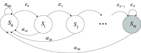
Figure 1: State diagram for the Markov chain for the UE power allocation scheme.

Formally, the state transition probability $\alpha_{ij}$ from the current state $S_{t}=i$ to next state $S_{t+1}=j$ is defined by,

$$\alpha_{ij} = {\rm Pr}(S_{t+1}=j|S_{t}=i)$$ (6)

$$= \begin{cases}1-\epsilon_{i},&\mbox{if ACK Received},\forall i,j=0\\ \epsilon_{i},&\mbox{if NAK Received},i\neq N,j=i+1,\\ &0\leq\epsilon_{i}\leq 1\\ \epsilon_{N},&\mbox{if NAK Received},i=N,j=N\\ 0,&\mbox{otherwise}\end{cases}$$ (7)

where $\epsilon_{i}$ is given by (1). The resulting state diagram is shown in Fig. 1. The state transition probability matrix $\mathbf{A}=[\alpha_{ij}]_{i,j=0}^{N}$ takes the form

$$\mathbf{A}=\left(\begin{array}[]{ccccc}1-\epsilon_{0}&\epsilon_{0}&0&\dots&0\\ 1-\epsilon_{1}&0&\epsilon_{1}&\dots&0\\ \ddots&\ddots&\ddots&\ddots&\ddots\\ 1-\epsilon_{N-1}&0&0&\dots&\epsilon_{N-1}\\ 1-\epsilon_{N}&0&0&\dots&\epsilon_{N}\\ \end{array}\right)$$ (8)

For a time homogeneous Markov chain, the steady state probability for state $j$, $\pi_{j}$ is defined by

$$\pi_{j}=\sum_{i\in\mathcal{S}}\alpha_{ij}\pi_{i}$$ (9)

where $\mathcal{S}$ defines the state space for the UE states.

Assuming $N_{0}=1$, for Rayleigh fading and state $i$, the outage probability is given by,

$$\epsilon_{i} = 1-\exp\Big{(}\frac{-(2^{R}-1)}{P_{i}}\Big{)}$$ (10)

After some algebraic manipulation, the required transmit power $P_{i}$ is calculated by,

$$P_{i}=\frac{1-2^{R}}{\log(1-\epsilon_{i})}$$ (11)

Note that other channel distributions, e.g., diversity reception or transmission with multiple receive and/or transmit antennas with single-stream transmission and $2\cdot d$ ($d$ is the number of active antennas) fold diversity, result in similar outage probability expressions, as in equation (27) in [12]:

$$\epsilon_{i}=P\left(d\frac{2^{R}-1}{P_{i}},d\right)$$ (12)

with the incomplete Gamma function $P(a,x)$ defined in [13, 6.5.1]. It is not easy to solve (12) with respect to $P_{i}$ due to the incomplete Gamma function.

From the transmit power for every state $i$, the average transmit power consumed is given by,

$$P_{a}=\sum_{i=0}^{N}P_{i}\pi_{i}.$$ (13)

IV Optimization Problem Formulation

The optimization problem is to compute a vector of power values $\mathbf{P}=[P_{0},P_{1},\dots P_{N}]$, which satisfies the constraints on packet dropping parameters and minimizes average system energy. The problem is mathematically formulated as,

$$\min_{\mathbf{P}}P_{a}$$ (14)

$$s.t. \begin{cases}\mathcal{C}_{1}:\gamma_{r}\leq\gamma,&0\leq\gamma\leq 1\\ \mathcal{C}_{2}:\epsilon_{N}\leq\epsilon_{out}&0\leq\epsilon_{out}\leq 1\end{cases}$$ (15)

$\mathcal{C}_{1}$ is the average packet loss constraint for the achieved average packet loss rate $\gamma_{r}$. From the state space model,

$$\gamma_{r}=\sum_{i=0}^{N}\epsilon_{i}\pi_{i}~{}.$$ (16)

The outage probability $\epsilon_{i}$ and the corresponding transmit power $P_{i}$ for a UE in state $i$ is computed such that the average packet dropping probability constraint $\mathcal{C}_{1}$ holds. For $i=N$, $\epsilon_{N}\leq\epsilon_{out}$ where $\epsilon_{out}$ is defined in (3). $\epsilon_{i}$ cannot be determined directly and needs to be optimized for the system parameters.

$$\epsilon_{i}=f(\gamma,N,\epsilon_{out},h_{X}(x),R)$$ (17)

where $h_{X}(x)$ is the fading channel distribution.

The optimization problem is to find $\epsilon_{i}$, $\forall i$ that results in minimum average power. If we choose $P_{i}$ too high for small states, the packets will more likely be transmitted too early at the expense of larger power budget without exploiting loss tolerance of the application and provide good (but unnecessary) QoE. On the other side, if $P_{i}$ is chosen too low in the beginning, the packets will be lost mostly and we have to transmit with much higher power to meet the forced condition that at least one packet has to be transmitted to avoid the sequence of $N$ lost packets.

IV-A Special Case $N=1$

Let us examine a special case with $N=1$. In this case, state transition probability matrix $\boldsymbol{A}$ reads,

$$\mathbf{A}=\left(\begin{array}[]{cc}1-\epsilon_{0}&\epsilon_{0}\\ 1-\epsilon_{1}&\epsilon_{1}\\ \end{array}\right)$$ (18)

Steady state transition probabilities for states $0$ and $1$ are calculated as,

$$\pi_{0}=\frac{1-\epsilon_{1}}{1+\epsilon_{0}-\epsilon_{1}}$$ (19)

$$\pi_{1}=\frac{\epsilon_{0}}{1+\epsilon_{0}-\epsilon_{1}}.$$ (20)

Computing $\gamma_{r}$ for $\epsilon_{1}=\epsilon_{out}$ and $\pi_{0}$ and $\pi_{1}$ calculated above, (16) yields

$$\gamma_{r}=\frac{\epsilon_{0}}{1+\epsilon_{0}-\epsilon_{out}}.$$ (21)

We can compute the value of $\epsilon_{0}$ in closed form that satisfies constraint $\mathcal{C}_{1}$ and $\mathcal{C}_{2}$ with equality. Solving (21) and $\mathcal{C}_{1}$ in (15) with equality,

$$\epsilon_{0}=(1-\epsilon_{1})\frac{\gamma}{1-\gamma}.$$ (22)

Then, we compute power levels $P_{0}$ and $P_{1}$ and resulting average power $P_{a}$ in closed form using (11) in (13). We numerically show in Section VI that the power levels computed in closed form for the boundary condition $\epsilon_{N}=\epsilon_{out}$ is not optimal for every value of $\epsilon_{out}$.

The expressions for the power levels cannot be obtained in closed form for $N>1$. The variables $\epsilon_{0},\epsilon_{1}\dots\epsilon_{N}$ are unknown and it is not possible to compute a unique set of $\epsilon_{i},\forall i$ in closed form that satisfies $\mathcal{C}_{1}$ in (15). The optimization problem in (14) is a combinatorial problem as it is hard to compute a unique solution in terms of $\epsilon_{i},\forall i$ due to sum of product term in (16). It is therefore, difficult to compute $\mathbf{P}$ that minimizes $P_{a}$ using convex optimization techniques.

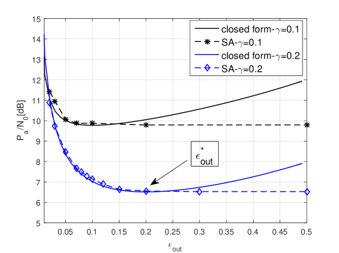
(a) Average power for both closed form solution and SA method.

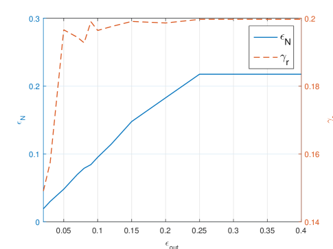
(b) Achieved $\gamma_{r}$ and $\epsilon_{N}$ for different $\epsilon_{out}$.

Figure 2: Performance of the proposed scheme for different packet loss parameters with $N=1$.

IV-B Optimization with Peak Power Constraint

Let us assume that we have a peak power constraint $P_{m}$ at the transmitter side. This implies that largest transmit power at the UE cannot exceed $P_{m}$ in any state $i$, regardless of the other problem constraints. Thus, peak power constraint is added to the constraints in (15):

$$\mathcal{C}_{3}:P_{i}\leq P_{m}, \forall i,j$$ (23)

where $\mathcal{C}_{3}$ represents the peak power constraint.

Lemma 2.

The peak power constraint $P_{i}\leq P_{m},\forall i,j$, reduces to $P_{N}\leq P_{m}$.

Proof.

From Lemma 1, $P_{i}\leq P_{i+1}$, $\forall i$. This implies, $P_{N}$ is the largest transmit power for any state. Constraining $P_{N}\leq P_{m}$ is therefore, enough to apply peak power constraint for the overall system. ∎

From Lemma 2, $P_{N}$ is constrained by $P_{m}$. However, $P_{N}$ is also constrained by the power resulting from system parameter $\epsilon_{out}$ ($\mathcal{C}_{2}$). This implies that the problem is only feasible if the solution satisfies both outage probability resulting from the peak power constraint and the outage constraint $\epsilon_{out}$. Denoting the power consumption from $\epsilon_{out}$ by $P_{out}$, the solution is feasible if

$$P_{out}\leq P_{N}\leq P_{m}.$$ (24)

V Stochastic Optimization

The combinatorial optimization problems which are not solvable with regular optimization techniques, can approximately be solved using stochastic optimization methods. There are a few heuristic techniques in literature to solve such problems like genetic algorithm, Q-learning, neural networks, etc. We use Simulated Annealing (SA) algorithm to solve the problem. The algorithm was originally introduced in statistical mechanics, and has been applied successfully to networking problems [9, 10].

In SA algorithm, a random configuration in terms of transition probability matrix $\boldsymbol{A}$ is presented in each iteration and the average power $P_{a}$ is evaluated only if constraints in (15) are met. If the evaluated $P_{a}$ is less than the previously computed best solution, the candidate set of outage probabilities $\epsilon_{i}$, $\forall i$ are selected as the best available solution. However, the candidate set $\epsilon_{i}$, $\forall i$ can be treated as the best solution with a certain temperature dependent probability even if the new solution is worse than the best known solution. This step is called muting and helps the system to avoid local minima. The muting occurs frequently at the start of the process as the selected temperature is very high and decrease as temperature is decreased gradually, where temperature denotes a numerical value that controls the muting process.

In literature, different cooling temperature schedules have been employed according to the problem requirements. The cooling schedule determines the convergence rate of the solution. If temperature cools down at a fast rate, the optimal solution can be missed. On the other hand, if it cools down too slowly, optimization requires large amount of time. In this work, we employ the following cooling schedule, called fast annealing (FA) [14]. In FA, it is sufficient to decrease the temperature linearly in each step $b$ such that,

$$T_{b}=\frac{T_{0}}{c_{\rm sa}\cdot b+1}$$ (25)

where $T_{0}$ is a suitable starting temperature and $c_{\rm sa}$ is a constant, which depends on the requirements of the problem. After a fixed number of temperature iterations, when muting ceases to occur completely, the best solution is accepted as optimal solution.

LABEL:algorithm.

VI Numerical Results

We perform numerical evaluation of the proposed scheduling scheme in this section. We consider a Rayleigh fading channel with mean $1$ for the point to point link. The noise variance $N_{0}$ equals one. Spectral efficiency $R$ equals 1 bits/s/Hz while peak power is set to a relatively high value of $20$ dBW for all numerical examples.

We study the effect of packet loss parameters on average power consumption for the special case $N=1$ in Fig. 2, where the results are evaluated using both closed form expressions derived in Section IV-A and the SA framework developed in Section V. Average transmit power is plotted for the fixed $N$ and $\gamma=0.1,0.2$ in Fig. 2(a). Note that $\epsilon_{out}=\epsilon_{N}$ in the closed form expression. Average power consumption is a convex function in $\epsilon_{out}$ for a fixed $\gamma$ and $N$, and a unique optimal $\epsilon_{out}$ can be seen. Let us call it $\epsilon_{out}^{*}$. If system parameter $\epsilon_{out}\leq\epsilon_{out}^{*}$, it results in high average power. However, if $\epsilon_{out}>\epsilon_{out}^{*}$, the system has more flexibility and it is optimal to set $\epsilon_{N}=\epsilon_{out}^{*}$ instead to save power. The optimized results with SA method match closely with the closed form results for $\epsilon_{out}\leq\epsilon_{out}^{*}$ which validate the accuracy of solution provided by SA algorithm. For $\epsilon_{out}>\epsilon_{out}^{*}$, SA method provides the optimal solution in contrast to the suboptimal solution where $\epsilon_{N}=\epsilon_{out}$ is enforced.

Fig. 2(b) confirms the results in Fig. 2(a) for the experiment conducted using SA algorithm. We plot $\epsilon_{N}$ (read on left y-axis) and the corresponding $\gamma_{r}$ values (read on right y-axis) for different values of $\epsilon_{out}$. When $\epsilon_{out}\leq\epsilon_{out}^{*}$, $\epsilon_{N}$ follows $\epsilon_{out}$ closely while $\gamma_{r}<\gamma$. When $\epsilon_{out}>\epsilon_{out}^{*}$, $\epsilon_{N}=\epsilon_{out}^{*}$ while $\gamma_{r}\to\gamma$. These results explain the average power optimization for SA algorithm in Fig. 2(a) that all degrees of freedom are sufficiently exploited at $\epsilon_{out}=\epsilon_{out}^{*}$ to optimize the energy consumption for a fixed $\gamma$ and $N$.

Fig. 3 compares the average power consumption for the case $N=1,2,3$ and $\gamma=0.2$. The power levels are optimized using Simulated Annealing algorithm. It is evident that $\epsilon_{out}^{*}$ and resulting average power is the same for all $N$. When $\epsilon_{out}\leq\epsilon_{out}^{*}$, an increase in $N$ for a fixed $\gamma$ helps to reduce average power consumption in general (specially at small $\epsilon_{out}$). More flexibility in packet dropping parameters provides more degrees of freedom and results in energy savings. When $\epsilon_{out}>\epsilon_{out}^{*}$, the effect of large $N$ vanishes and power saving depends solely on average packet dropping parameter.

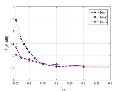
Figure 3: Average power as a function of packet loss parameters for different $N$. $\gamma$ is fixed to 0.2.

VII Conclusion

We consider energy efficient scheduling and power allocation for the loss tolerant applications. Data loss is characterized as a function of average and successive packet loss, and the probability that successive packet loss is not guaranteed. These parameters jointly define the QoE and context for an application. In contrast to average packet loss parameter, other loss parameters depend on the packet loss patterns without actually changing the number of lost packets. By considering bursty packet loss a form of contextual information, we provide another degree of freedom in the scheduling algorithm which can be exploited to reduce energy consumption. Without CSIT, we formulate the average power optimization problem as a function of data loss parameters. The optimization problem is a combinatorial optimization problem and requires stochastic optimization technique to solve it. We compute closed form expressions of average power as a function of system parameters for the special case $N=1$ and compare it with the solution obtained from simulated annealing algorithm. Both of the results match up to a point and diverge after words due to inaccurate assumptions for the closed form solution. However, the matching of both results validate the solution provided by simulated annealing algorithm. For $N\geq 1$, we numerically quantify the energy savings for increased flexibility in successive packet loss tolerance parameter.

References

- [1] T. Villa, R. Merz, R. Knopp, and U. Takyar, “Adaptive modulation and coding with hybrid-ARQ for latency-constrained networks,” in European Wireless Conference, April 2012, pp. 1–8.
- [2] J. Choi and J. Ha, “On the energy efficiency of AMC and HARQ-IR with QoS constraints,” IEEE Trans. Vehicular Technology, vol. 62, pp. 3261–3270, 2013.
- [3] M. M. Nasralla, C. T. E. R. Hewage, and M. G. Martini, “Subjective and objective evaluation and packet loss modeling for 3D video transmission over LTE networks,” in International Conference on Telecommunications and Multimedia (TEMU), Heraklion, Crete, Greece, July 2014.
- [4] Z. Zou and M. Johansson, “Deadline-constrained maximum reliability packet forwarding with limited channel state information,” in IEEE Wireless Communications and Networking Conference (WCNC), April 2013, pp. 1721–1726.
- [5] A. Dua, C. W. Chan, N. Bambos, and J. Apostolopoulos, “Channel, deadline, and distortion (CD2) aware scheduling for video streams over wireless,” IEEE Trans. Wireless. Communications, vol. 9, no. 3, pp. 1001–1011, Mar. 2010.
- [6] L. Sequeira, J. Fernandez-Navajas, L. Casadesus, J. Saldana, I. Quintana, and J. Ruiz-Mas, “The influence of the buffer size in packet loss for competing multimedia and bursty traffic,” in International Symposium on Performance Evaluation of Computer and Telecommunication Systems, Toronto, Canada, July 2013.
- [7] F. Liu, T. H. Luan, X. S. Shen, and C. Lin, “Dimensioning the packet loss burstiness over wireless channels: a novel metric, its analysis and application,” Wireless Communications and Mobile Computing, 2012.
- [8] M. J. Neely, “Intelligent packet dropping for optimal energy-delay tradeoffs in wireless downlinks,” IEEE Trans. on Automatic Control, vol. 54, no. 3, pp. 565–579, March 2009.
- [9] M. M. Butt and E. A. Jorswieck, “Maximizing system energy efficiency by exploiting multiuser diversity and loss tolerance of the applications,” IEEE Trans. Wireless Communications, vol. 12, no. 9, pp. 4392–4401, 2013.
- [10] M. M. Butt, E. A. Jorswieck, and A. Mohamed, “Energy and bursty packet loss tradeoff over fading channels: A system-level model,” IEEE Systems Journal, vol. PP, no. 99, pp. 1–12, 2016.
- [11] P. Whittle, “Restless bandits: Activity allocation in a changing world,” Journal of Applied Probability, vol. 25, pp. pp. 287–298, 1988.
- [12] E. A. Jorswieck and H. Boche, “Outage probability in multiple antenna systems,” European Trans. on Telecom., vol. 18, pp. 217–233, 2007.
- [13] M. Abramowitz and I. A. Stegun, Handbook of Mathematical functions. Dover Publications, 1970.
- [14] H. Szu and R. Hartley, Physics Letters A, no. 3, June.